Psychophysiology-aided Perceptually Fluent Speech Analysis of Children Who Stutter

Abstract.

This first-of-its-kind paper presents a novel approach named PASAD that detects changes in perceptually fluent speech acoustics of young children. Particularly, analysis of perceptually fluent speech enables identifying the speech-motor-control factors that are considered as the underlying cause of stuttering disfluencies. Recent studies indicate that the speech production of young children, especially those who stutter, may get adversely affected by situational physiological arousal. A major contribution of this paper is leveraging the speaker’s situational physiological responses in real-time to analyze the speech signal effectively. The presented PASAD approach adapts a Hyper-Network structure to extract temporal speech importance information leveraging physiological parameters. In addition, a novel non-local acoustic spectrogram feature extraction network identifies meaningful acoustic attributes. Finally, a sequential network utilizes the acoustic attributes and the extracted temporal speech importance for effective classification. We collected speech and physiological sensing data from $73$ preschool-age children who stutter (CWS) and who don’t stutter (CWNS) in different conditions. PASAD’s unique architecture enables visualizing speech attributes distinct to a CWS’s fluent speech and mapping them to the speaker’s respective speech-motor-control factors (i.e., speech articulators). Extracted knowledge can enhance understanding of children’s fluent speech, speech-motor-control (SMC), and stuttering development. Our comprehensive evaluation shows that PASAD outperforms state-of-the-art multi-modal baseline approaches in different conditions, is expressive and adaptive to the speaker’s speech and physiology, generalizable, robust, and is real-time executable on mobile and scalable devices.

1. Introduction

Approximately $5$ percent of all children go through a period of stuttering, and $1$ percent suffer from long-term stuttering (stu, 2022). Stuttering first emerges in preschool years and, for those children who develop chronic stuttering, it can lead to life-long adverse consequences and compromised wellbeing (Carter et al., 2017). Although stuttering is characterized by audible speech disfluencies that disrupt ongoing speech production and break the rhythm of speech, it has long been proposed that these disruptions are the result of underlying differences in speech-motor-control (SMC) processes (Amster and Starkweather, 1987) that are present in the fluent speech of people who stutter (e.g., (Heyde et al., 2016; Usler et al., 2017)).

Speech scientists or clinicians aim to improve the stuttering individual’s SMC, which is impacted by the speaker’s articulators, such as jaw or tongue position. The current SMC measuring process is manual, done only through fluent speech repetitions of fixed phrases (Tumanova et al., 2020b; Van Lieshout and Namasivayam, 2010), and then comparing the spectral attributes’ deviation across all repeats. It is only an aggregated measure, cannot evaluate spontaneous speech, and needs manual effort from trained individuals. Hence, there is a critical need for an automated approach to identify and visualize the fine-grain, second-by-second, and personalized deviation in the spectral-parameters-of-interest (i.e., speech features/attributes discussed in section 7.2) of a stuttering individual’s fluent speech from others.

Importantly, preschool-age is when children rapidly develop their language and SMC. Several studies (Curlee and Yairi, 1997; Yaruss et al., 2002; Craig et al., 1992) have established that early-age interventions are highly effective and more frequently result in permanent remissions of stuttering (Curlee, 1993a, b). Thus, this study is interested in examining (i.e., detecting and visualizing the differences in) perceptually fluent speech of children who stutter (CWS) and don’t stutter (CWNS).

However, unlike stuttering or speech disfluency detection tasks, the difference in fluent speech between CWS and CWNS is subtle and perceptually indifferentiable, making this paper’s task challenging; and conventional machine learning (ML)-based speech analytics approaches fail to achieve high efficacy (table 2).

Interestingly, speech science studies have shown that situational physiological responses (i.e., arousal) affect children’s SMC, and such effect is even prominent in CWS’s SMC (Bauerly and Bilardello, 2021; Erdemir et al., 2018; Diehl et al., 2019; Arenas and Zebrowski, 2013; Zengin-Bolatkale et al., 2015). A recent work (Sharma et al., 2022) showed that CWS indeed show fine-grain, second-by-second differences (not necessarily always higher) in situational arousal responses than their non-stuttering peers. Notably, arousal is a continuous and persistent state that measures the intensity of the affective state ranging from calm to highly excited or alert (Bradley and Lang, 2007). Based upon these findings, a major contribution of this work is our use of the speaker’s situational physiological arousal in real-time to analyze the speech signal effectively, which we demonstrate significantly improves the accuracy of classifying perceptually fluent speech as coming from CWS or CWNS.

Conventional sequential classifiers (e.g., LSTM, GRU) used in speech analysis literature (Shewalkar, 2019; Salekin et al., 2017) use an identical set of network weights in each timestamp. However, children’s speech acoustic get affected by their psychophysiology (Bauerly and Bilardello, 2021; Erdemir et al., 2018; Arenas and Zebrowski, 2013; Zengin-Bolatkale et al., 2015), meaning each timestamp’s acoustic analysis should be adaptive to the speaker’s physiological response on that timestamp, that the conventional classifiers’ static network weights fail to facilitate.

The paper presents a first-of-its-kind Psychophysiology aided Speech Attribute Detection (PASAD) approach that differentiates perceptually fluent speech from CWS vs. CWNS. PASAD presents a unique HyperNetwork (Ha et al., 2016) adaption (section 5.2) that leverages the speaker’s real-time psychophysiological parameters to update a sequential speech classifier’s network weights dynamically. Hence, the classifier has a new set of weights at each timestamp, meaning it can focus on (i.e., analyze) different aspects of speech acoustic conforming to the speaker’s real-time psychophysiology.

We use a Mel-spectrogram representation of speech and, following speech science literature, use a robust (and unbiased) change-score representation of physiological parameters as psychophysiological features (section 4.1). Spectrogram features are distributed over different time and frequency ranges. Conventional convolution layers only capture feature-relations within a small neighborhood (i.e., the area of a kernel). Thus, they require a deep network structure to capture the features-relations in farther locations, which is difficult for limited data applications typical in the speech health domain. PASAD uses a novel speech spectrogram embedding extraction network block (section 5.3) that effectively captures the long-range spatial-temporal relations of different frequencies across time. Such speech attributes are effective in understanding the important frequency bands (i.e., formants), ergo, the SMC differences (sections 7).

Later, utilizing machine learning (ML) interpretation techniques, we visualize the distinct speech attributes of CWS that are indicative of their SMC differences from the CWNS. Conventional sensor data integration approaches concatenate the multi-modal sensing data within their network architectures and generate inferences utilizing the integrated information. Hence, it is difficult to identify the independent contribution of one modality from such architectures utilizing ML interpretation techniques. PASAD’s unique architecture utilizes only speech information for classification inference generation, enabling using ML interpretation techniques like Kernel SHAP (Lundberg and Lee, 2017) to extract and visualize the distinct speech attributes present in CWS’s speech and their corresponding SMC factors (discussed in sections 5 and 7).

In summary, the contributions of this paper are:

• Paper’s Task: This is the first work that enables automated, fine-grain, second-by-second, and personalized deviation detection and visualization in the spectral-parameters-of-interest (discussed in section 7.2) of a CWS’s ‘fluent speech’ from others. The presented approach is not constrained by fixed phrases and works for spontaneous speech. Only a limited number of studies in speech literature evaluated pre-school children’s speech. It is the age at which children rapidly develop their language, SMC, and emotion regulation and when the interventions are most effective, making the presented paper’s findings highly impactful.

• Classification: Presented first-of-its-kind PASAD approach uses a novel ‘speech spectrogram embedding extraction block’ that extracts meaningful long-range spatial-temporal relations of speech frequencies as attributes from each timestamp’s speech, where the developed novel Hyper-LSTM unit (section 5.2) dynamically priorities the attributes taking the speaker’s real-time psychophysiology into account.

  PASAD utilizes the speaker’s physiological response for effective acoustic analysis, and it makes CWS vs. CWNS classification decisions using only speech information (detail discussion is in section 6.6); ergo, it is not a multi-modal sensor data integration approach, rather a unique speech analysis approach that leverages multi-modal information, which means multi-modal approaches are not PASAD’s competitors or true baseline. However, for a comprehensive comparison, this paper compares PASAD with multiple multi-modal classifiers taking both speech acoustics and physiological parameters as input, and speech-classifiers only taking speech acoustics as input; all of which PASAD outperforms (section 6.1). PASAD’s higher performance demonstrates that it can effectively leverage the dynamic nature of speech attributes conforming to the stuttering speaker’s situational emotional reactivity.

• Our comprehensive evaluations demonstrate that PASAD is expressive and adaptive to speaker’s speech and physiological parameter changes (section 6.5), it utilizes only speech information in the class inference generation (section 6.6), it is generalizable to different unseen age and sex groups (section 6.7) and is real-time executable in resource constraint devices, such as jetson nano and smartphones (section 6.8).

• Datasets: To our knowledge, no existing dataset contains both speech and physiological parameters of CWS and CWNS. We collected two first-of-their-kind datasets, ‘stress-speech dataset’ and ‘narrative-speech dataset’ comprising CWS and CWNS’s perceptually fluent speaking and physiological parameters in stressful condition and spontaneous narration task, respectively. The narration task is linguistically and cognitively demanding since the children develop new contexts and articulate them in speech. It may elicit different physiological responses in CWS vs. CWNS (Zengin-Bolatkale et al., 2018). Two datasets comprise pre-school age $73$ participants ($34$ CWS and $39$ CWNS). Each dataset contains children’s speech and their physiological parameters: electrodermal activity (EDA), heart rate (HR), respiratory rate (RSP-rate), and respiratory amplitude (RSP-amp). Notably, the physiological parameters of the datasets and their difference between CWS and CWNS have recently been published in our previous work. However, the speech content, which is the focus of this paper, is unique and yet unpublished; notably, anonymized data will be made public with the published paper.

• Visualization: PASAD’s unique architecture enables extraction and visualization of distinct speech attributes present in CWS’s speech. It is important to note that we adhere to the speech representations or features evaluated in speech-science so that speech scientists or clinicians can use PASAD’s visualizations. Our discussion in section 7.3 demonstrates that the speech articulators (e.g., jaw, tongue), i.e., the SMC factors responsible for a CWS’s fluent speech (i.e., spectral-parameters-of-interests’) deviation are identifiable from our visualization. The presented PASAD and its visualization would enable remote, continuous, and real-time assessment of stuttering children’s speech articulation and SMC and may lead to personalized interventions.

Rest of the paper is organized as follows:

Section 2 discusses the related work and background on stuttering individuals’ speech and physiological parameters. Section 3 discusses the dataset and data collection procedures. Section 4 discusses the data preprocessing and feature extractions. Section 5 presents the developed PASAD approach. A comprehensive evaluation of the PASAD approach and its characteristics are discussed in section 6. Section 7 presents the ML interpretation generation of PASAD’s inferences, and provides a detailed interpretation discussion. Lastly, sections 8 and 9 summarize the study observations, broader impact and give a conclusion.

2. Related Work and Background Discussion

Studies in Speech Science.

Physiological arousal-related differences in SMC have been observed in the adults who stutter (AWS) and don’t stutter (AWNS) (Arenas and Zebrowski, 2013; Caruso et al., 1994; van Lieshout et al., 2014; Jackson et al., 2016). However, the knowledge of the effects of arousal on the AWS cannot be extended to young children as they undergo rapid development of many vital processes (e.g., cognitive growth, emotional regulation, and language acquisition) in their preschool-age years. Preschool age is also characterized by immature SMC that continues to develop well into the school-age years (Walsh et al., 2006; Smith et al., 2005). Given the immature SMC and less developed emotion regulation skills of preschool-age children, they may experience greater effects of physiological arousal on their speech than adults. Yet, to our knowledge, only limited research examined the effects of physiological arousal on the speech characteristics of young children. According to a recent study (Tumanova et al., 2020b), CWS demonstrate less mature SMC (i.e., less stable speech construction) than CWNS in emotionally arousing states. Despite this emerging evidence, the effects of emotional processes on perceptually fluent speech in CWS and CWNS are still not well understood. Moreover, though the above-mentioned studies established that on the aggregated level (through statistical analysis), CWS and CWNS show a difference in SMC while fluently repeating specific phrases, specifically in high-arousal situations; the presented study is the first to develop automated, second-by-second, and personalized assessment approach, and extends the previous findings by establishing the presence of SMC deviations even in the CWS’s spontaneous speech.

Machine Learning on Stuttering Speech Studies State-of-the-art ML studies on the stuttering population focus on detecting various stuttering disfluency events, such as repetition and prolongation of sounds/syllables, tension-filled pauses, and interjections. Ravikumar et al. (Ravikumar et al., 2008, 2009) evaluated MFCC speech features and SVM classifier to detect syllable repetitions. Recent studies are leveraging deep learning approaches. Kourkounakis et al. (Kourkounakis et al., 2020) developed a residual network (ResNet) and Bidirectional LSTM model, which took spectrogram as input to detect stuttering events. Another study (Sheikh et al., 2021) utilized a time-delay neural network (TDNN) taking MFCC features to detect stuttering events. The majority of the stuttering speech processing works have used the UCLASS dataset (Howell et al., 2009). It contains reading, monolog, and conversation speech containing stuttering events (e.g., repeating parts of words, stretching a sound out for a long time, or having a hard time getting a word out) from participants aged $5$ to $47$ years. Unlike the UCLASS dataset, the data used for this paper are perceptually fluent speech from preschool-age CWS and CWNS ($3$-$5$ years of age). To the best of our knowledge, no study has developed ML classification approaches to differentiate perceptually fluent speech of CWS vs. CWNS.

Speech Features in Stuttering and Arousal Studies Speech science studies have evaluated the fundamental frequency $F0$ and the first four formant frequencies to examine the SMC both in emotional stimuli scenarios and for stuttering individuals.

The fundamental frequency $F0$ approximates the periodicity of vibration of the speaker’s vocal cord (Guo et al., 2007; Guo-an, 2011). Studies reported that $F0$ contains information about the speaker’s emotional state (Protopapas and Lieberman, 1997; Fuller et al., 1992; Hecker et al., 1968). Stuttering and non-stuttering adults show difference in $F0$ while fluently uttering vowels (Natke and Kalveram, 2001; Salihovic et al., 2009). Notably, lower SMC is positively correlated with higher $F0$ variability (Robb and Saxman, 1985).

Formants are resonance frequencies of the vocal tract. Formants are measured as peak points of the amplitude in the frequency spectrum (discussed in section 4.2). Formally they are indicative of time-dependent positions of speech articulators, e.g., tongue, lips, velum, and jaw (Mermelstein, 1967; Ladefoged et al., 1978).

Studies have shown that stress stimuli cause pharyngeal constrictions and shorting of the vocal track in AWS. This leads to a rise in the first formant and a fall in the second formant values and narrow formant bandwidths (Scherer et al., 1991; Banse and Scherer, 1996; Protopapas and Lieberman, 1997). Additionally, the difference in the first formant is observed in AWS vs. AWNSs’ speech in stress conditions (Caruso et al., 1994). Second format frequency fluctuation reflects vocal tract stability (Gerratt, 1983) as it relates to the tongue position in the mouth. It has been used to assess motor control of stuttering adults (Robb et al., 1998), and children (Bauerly et al., 2019). Studies (Scherer, 2013) have found significant differences in the second formant values for vowels and third formant frequency fluctuations (Giannakakis et al., 2019) between the neutral and aroused utterances. Hence, the formants are important features in a stuttering individual’s speech analysis.

Additionally, Mel-frequency cepstral coefficient (MFCC) and zero crossing rate (ZCR) features have been leveraged in speech emotion detection (Partila et al., 2015; Salekin et al., 2017; Kurniawan et al., 2013) of CWS and CWNS.

Physiological Parameters in CWS vs. CWNS There is limited research that examines the physiological parameters of CWS vs. CWNS. Recent studies (Zengin-Bolatkale et al., 2018; Tumanova et al., 2020a; Sharma et al., 2022) have shown significant skin conductance (EDA), heart rate (HR), and respiratory effort (RSA) differences in CWS and CWNS in different conditions. A recent study (Tumanova et al., 2020a) showed that during stress-inducing conditions, the CWS exhibited a higher heart rate (HR) and a lower RSA than the CWNS. A study (Villegas et al., 2019) on AWS has developed a multi-layered perceptron (MLP) neural network-based stuttering disfluency event classification system that takes respiration signals as input. On the contrary, this first-of-its-kind study leverages CWS and CWNS’s physiological parameters in ML classifiers to understand their normally fluence speech differences.

3. Dataset Description and Collection Procedure

We collected data from preschool-age children in two settings. Due to the nature of the tasks the participants were engaged in, we refer to the first setting dataset as the “stress-speech dataset” and the second dataset as the “narrative-speech dataset” throughout the manuscript. Data collection with this very young population can be difficult as they may refuse to do tasks. Presented clinical data collection took multiple years for our multi-disciplinary team.

Participants Description : Participants were between 3-5 years of age. The X University Institutional Review Board approved the study. Informed consent by parents and verbal assent by children were obtained. Participants’ speech and language skills were assessed using standardized speech articulation and language measures. Participants’ speech fluency was assessed to diagnose developmental stuttering using evidence-based diagnostic criteria (Yaruss et al., 1998). All participants had English as their primary language, age-appropriate speech articulation, and language scores, and passed a pure-tone hearing screening.

Stress-speech Dataset has $38$ participants. $18$ children ($16$ males and $2$ females, mean age $4$ years $5$ months) were CWS, and $20$ were CWNS ($17$ males and $3$ females, mean age $4$ years $6$ months). Narrative-speech Dataset has $35$ different participants. $16$ children ($13$ males and $3$ females, mean age $3$ years $11$ months) were CWS. Other $19$ were CWNS ($12$ males and $7$ females, mean age $4$ years $1$ month).

Extracted Physiological Sensors and Parameters: The respiratory, electrodermal, and cardiac activity were acquired simultaneously using the Biopac MP150 hardware system (bio, 2016) and acqknowledge software (ver. 4.3 for PC, Biopac). Hypoallergenic electrodes were attached to the skin of the distal phalanges of the participants’ index and middle finger of the left hand for the acquisition of electrodermal activity (EDA) and to the skin at the suprasternal notch of the rib cage and at the 12th rib laterally to the left for the acquisition of the electrocardiogram (ECG) (Venables and Christie, 1980). A strain gauge transducer designed to measure respiratory-induced changes in thoracic or abdominal circumference (model TSD201, Biopac Systems, Inc.) was used to record respiratory effort (RSP). The transducer was positioned around the participants’ chest. All signals were sampled at $1250$ Hz. We extract the respiratory rate (RSP-rate) and respiratory amplitude (RSP-amp) (Schneider et al., 2003) from raw RSP signal and heart rate (HR) from raw ECG signal. Hence, the raw physiological parameters extracted and utilized are EDA, HR, RSP-rate, and RSP-amp.

Extracted Speech Signal: In each of the data collection setups, a Shure sm58 microphone (shu, 2022) was positioned approximately 50 cm (1.64 feet) from the participant’s mouth to record the participant’s speech. The speech was collected with a 10kHZ sampling rate.

3.1. Sensor Data Collection Procedure

Both datasets’ data collection comprised a baseline and an experimental condition; the baseline was the same in both.

Baseline Condition (Common): For both datasets, to establish a pre-experimental baseline for each participant’s resting psychophysiological parameters, participants viewed an animated screensaver of a three-dimensional fish tank for four minutes. This procedure has been successfully implemented in prior studies to establish baseline psychophysiological levels in preschool-age children (Jones et al., 2014).

Stress-speech Experimental Condition: This data collection session lasted approximately $10$ minutes. Participants were shown $10$ negatively-valenced pictures from the International Affective Picture System (Lang et al., 1997) and were asked to repeat a simple phrase “Buy Bobby a puppy” (BBAP) three times after each picture shown. Participants (both CWS & CWNS) did not show any stuttering events during this task, and their speech was entirely fluent.

Narrative-speech Experimental Condition: The session lasted approximately 12 minutes and comprised a picture description task. Participants were shown pictures from a wordless storybook (Frog Goes to Dinner by Mayer (1974)). To keep the narrative elicitation procedure consistent between participants, the examiner was only allowed to prompt the participant by saying, “Let’s look at this picture. Tell me what is happening here.” CWS participants did show some stuttering events during this task, but they were infrequent. On avg., 97% of their words were produced fluently. This study evaluated only the fluent speech portions.

4. Features Extraction

In the stress-speech dataset, each BBAP utterance takes 3-5 sec. Since, during SMC assessment, the existing speech science studies evaluate complete utterances, to be consistent, this paper detects CWS vs. CWNS speech from $5$ sec windows. During stress-speech dataset evaluation, each 5 sec window comprises one BBAP utterance. Since narrative-speech is spontaneous, we segmented the 12 min experimental session (section 3.1) into 5 sec windows, eliminated all silent windows and windows containing stuttering/speech-disfluency events, and evaluated the rest. From the stress-speech dataset, a total of $1117$ non-overlapping $5$ sec windows ($581$ from CWS and $596$ from CWNS), and from the narrative-speech dataset, $3771$ non-overlapping $5$ sec windows ($1648$ from CWS and $2123$ from CWNS) were extracted. Each of the $5$ sec speech and physiological signal was divided into $19$ segments with $500$ ms duration and $250$ ms overlap, and physiological (section 4.1) and acoustic (section 4.2) features are extracted from the $500$ ms segments.

4.1. Physiological Features

Two categories of physiological features: (a) raw features and (b) changed-score features are extracted from the $500$ ms segments. The presented approach uses change-score features as the input physiological feature representation.

Raw physiological features:

Following the previous studies (Partila et al., 2015; Salekin et al., 2017; Kurniawan et al., 2013), we consider the low-level descriptor (LLD) features: heart rate (HR), electrodermal activity (EDA), respiratory rate (RSP-rate), and respiratory amplitude (RSP-amp) from each $500$ ms segments (sections 2 & 3). Six high-level descriptors (HLD) functionals: min, max, std, var, mean, and median are applied on the LLDs to extract the feature representation of each $500$ ms segment. In total, we extract $19\times 24$ raw physiological features from the $5$ sec event detection window.

Change-score Features:

Following studies on CWS’s physiological response (Sharma et al., 2022; Jones et al., 2017), we extract change-scores of HR, EDA, RSP-amp, and RSP-rate LLD features from each $500$ ms segment. Change-scores are the differences between the $500$ ms physiological signal segments in different speech conditions from the same individual’s avg. physiological signal in the baseline (i.e., resting) condition. In this study, the differences (i.e., change-scores) are measured by two matrices: cosine similarity and the euclidean distance. For each of the four LLD features HR, EDA, RSP-amp, and RSP-rate, we calculate two difference measures, totaling eight change-score features extracted from each $500$ ms segment. We extract $19\times 8$ change-score features from the $5$ sec window.

An individual may have an above-average physiological response (e.g., HR, EDA) in the baseline condition. However, a classifier trained on raw physiological features would be unaware of such exceptions and infer the individual’s neutral state as a stress state. The change-score features eliminate such biases.

4.2. Acoustic Features

The presented approach extracts a Mel-spectrogram from each $500$ ms segment and detects $5$ sec speech categories (CWS vs. CWNS) from the sequence of $19$ spectrograms. To compare with speech literature, we also extracted and evaluated raw acoustic features.

4.2.1. Mel-Spectrogram

The spectrogram represents the speech’s strength (i.e., energy) over time at various frequencies. We extract a Mel-spectrogram from each $500$ ms audio segment. It represents the acoustic signal on the Mel scale. The Mel Scale is a logarithmic transformation of a signal’s frequency, such that sounds within an equal distance on the Mel Scale are perceived as equal to humans. State-of-the-art acoustic analysis studies (Suhas et al., 2020; Bhattacharya and Shahnawaz, 2021; Dieleman and Schrauwen, 2014) suggested that the use of Mel-spectrogram leads to improved accuracy than the conventional spectrograms. During the time-to-frequency domain transformation, the length of the FFT window is 2048 sample points, and the hop length is 512 sample points. The desired frequency resolution governs the choice of FFT bins. Short-term spectral measurements are carried out for smaller window sizes of $20$ ms (Deller et al., 2000; Benesty et al., 2008). This controls the trade-off between the time and frequency resolution for the signal.

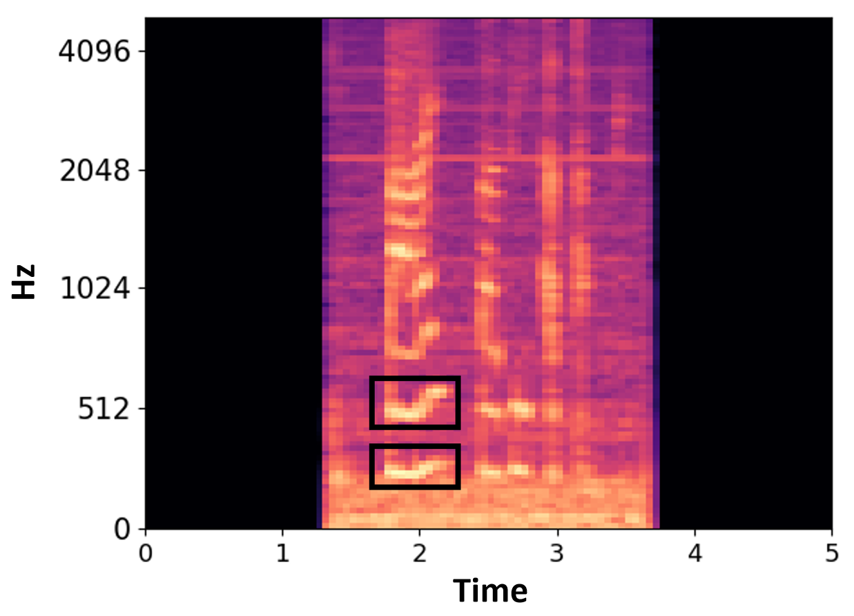
Figure 1. Mel-spectrogram for a $5$ sec speaking window

Fig. 1 shows a Mel-spectrogram of a ‘Buy bobby a puppy’ utterance from a participant in the stress-speech dataset. Time and frequency are along the horizontal and vertical axis. Amplitude is represented by the dark-to-bright color, where the brighter pixels represent higher amplitude regions.

Mel-spectrogram contains information about the acoustic features studied by speech pathologists. For example, the $250$-$400$Hz region represents the children’s speech fundamental frequency $F0$ information. Formants are seen as the bright bands on the Mel-spectrogram. They are the peak points of the amplitude in the frequency spectrum. Formally they are indicative of time-dependent positions of speech articulators, e.g., tongue, lips, velum, and jaw (Mermelstein, 1967; Ladefoged et al., 1978). The first two formants are highlighted in the bounding boxes in Fig. 1. These formants and their relations represent speech signal characteristics, such as fundamental frequency $F0$, speech formants distribution, etc. At each timestamp, a Mel-spectrogram from a $500$ ms speech signal is input to the detection network’s ‘Feature-Extractor’ block (section 5.3).

4.2.2. Raw Acoustic Features:

This paper also evaluates the efficacy of using raw acoustic features. The first 13- Mel-frequency cepstral coefficient (MFCC), Zero crossing rate, fundamental frequency, and first four formant frequencies, and their delta coefficients extracted from each $500$ ms speech segment as the low-level descriptor (LLD) features. Next, the 6 high-level descriptors (HLD) functionals: min, max, std, var, mean, and median are applied to the LLDs to extract the feature representation of the $500$ ms segment.

5. Methodology: Psychophysiology-aided Speech Attribute Detection (PASAD)

This section presents our approach. An overview of PASAD’s network architecture design choices that enable dynamic extraction of temporal speech importance according to the speaker’s situational physiological response and visualization of the independent contribution of speech attributes in differentiating fluent speech of CWS vs. CWNS is discussed below. In later sections 5.2-5.5, different components of PASAD are discussed in detail.

5.1. Overview of the PASAD Approach and Design Choices

PASAD utilizes a novel Hyper-LSTM unit (shown in Fig. 2(b)) that includes four components: reference-extractor, feature-extractor, auxiliary $LSTM_{aux}$, and main $LSTM_{main}$. At each timestamp $t$, the feature-extractor and the reference-extractor block generate the embeddings of the $500$ ms spectrogram and psychophysiological parameters. Notably, CWS vs. CWNS classification inferences generating main-$LSTM_{main}$ takes only the spectrogram embedding as input.

Conventional LSTM network unit (Cheng et al., 2016) comprises four gates. The forget gate $W_{f}$ decides how much information from the previous timestamps should be kept. Both input gate $W_{i}$ and new-memory gate $W_{g}$ quantify the importance of the new input $x_{t}$ at timestamp $t$ and updates the cell state $c_{t}$ accordingly. The output gate $W_{o}$ decides the new hidden state $h_{t}$, considering $c_{t}$, $h_{t-1}$, and $x_{t}$. Combined, these gates identify the importance of the input $x_{t}$ compared to the overall sequential data. These gate weights are learned during training, and they are fixed across timestamps during evaluation. Hence, LSTM is incapable of dynamic input importance extraction.

In the presented Hyper-LSTM unit (Fig. 2(b)), the gate weights of $LSTM_{main}$ are flexible. At each timestamp, the auxiliary $LSTM_{aux}$ takes the psychophysiological parameters and spectrogram embedding to dynamically generate the $LSTM_{main}$’s gate weights for that corresponding timestamp. This means that the $LSTM_{main}$ network generates the class inferences, taking fluent speech spectrograms as input, where the $LSTM_{main}$’s gate weights that identify each timestamp’s speech information importance are adaptive and generated utilizing the speaker’s physiological parameters (i.e., indicative to their arousal states). Therefore, PASAD performs classification utilizing only speech information (further discussed in section 6.6). However, dynamic $LSTM_{main}$-gate-weight generation enables important speech acoustic information extraction adaptive to the speaker’s real-time psychophysiology, hence resulting in better CWS vs. CWNS classification performance. Such architecture enables applying SHAP on the $LSTM_{main}$ network and identifying the importance of different frequencies (and corresponding amplitudes) across time from the fluent speech spectrogram in differentiating CWS vs. CWNS (section 7).

Another contribution of the presented approach is the effective spectrogram embedding generation. The presented Feature-Extractor block (section 5.3) is a novel integration of a non-local network followed by convolution layers that extracts the pairwise and unary relations of all frequencies across time.

PASAD’s overall architecture is a bi-directional HyperNetwork structure shown in Fig. 2(a). The components of the network are discussed below.

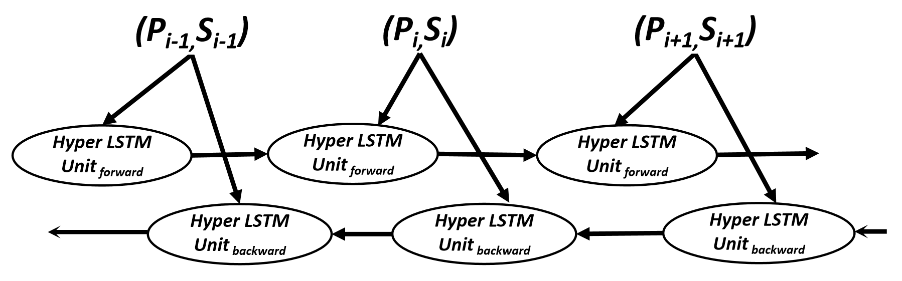
(a) Overall Architecture

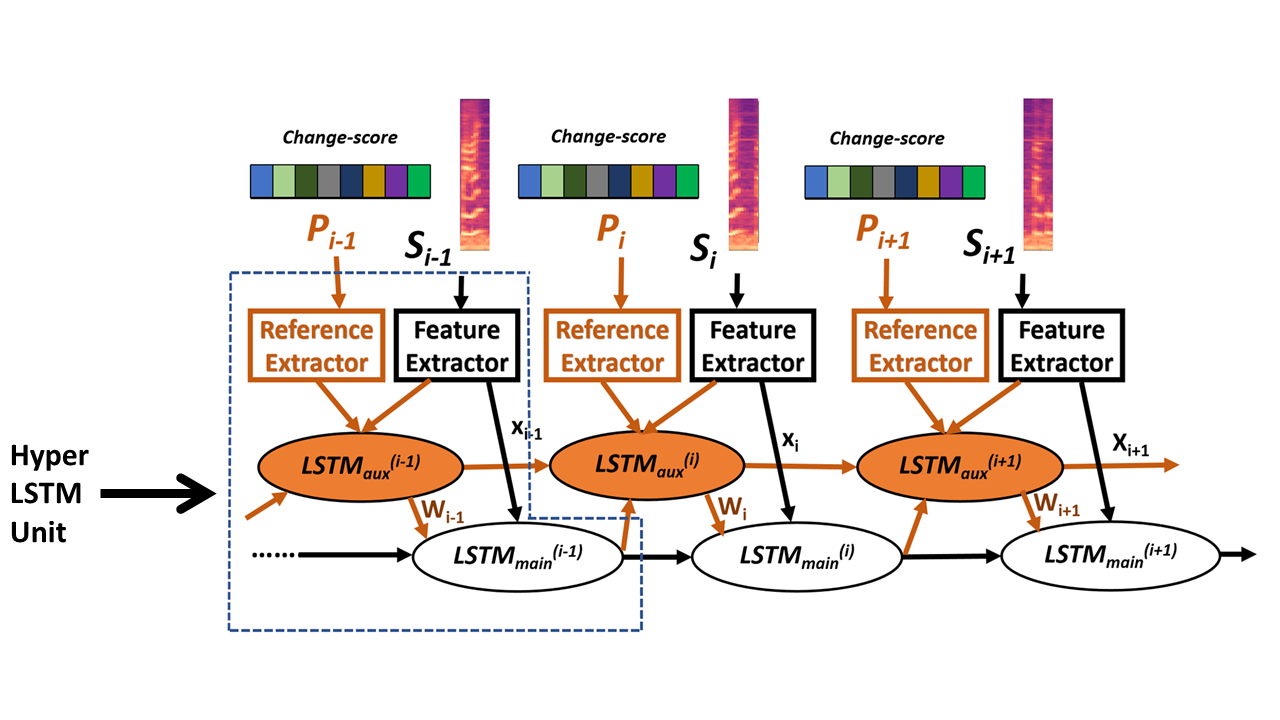
(b) Hyper LSTM unit Architecture

Figure 2. Diagram of the Bi-directional HyperLSTM multi-modal sensor data integration approach. Fig (a) shows the overall architecture. Fig (b) shows the HyperLSTM unit comprising of a $LSTM_{main}$ that takes the audio spectrogram features as input for decision making and a $LSTM_{aux}$ that generates the four gates weights on the $LSTM_{main}$ unit at each timestamp.

5.2. Hyper-LSTM Unit

Recurrent neural networks (e.g., RNNs, LSTMs) have been used in literature to capture the sequential temporal patterns of speech (Wang et al., 2020; Lu et al., 2018). LSTM can be viewed as a forward neural network that has the same weight at each layer. While weight-sharing between layers allows LSTM to share information across time and analyze sequential data, it has limited expressiveness/adaptability. HyperLSTM (Ha et al., 2016) overcomes the limitation by utilizing an auxiliary LSTM to dynamically generate the weights used by the main LSTM at each timestamp and for each input sequence. Hence, it generates the abstraction of having different weights at each layer adaptive to the input sequence.

Since the variation of speakers’ arousal affects the speech characteristics, it is crucial to extract salient speech patterns contingent on their physiological parameters in different timestamps for effective speech attribute classification. In the presented HyperLSTM structure (Fig. 2(a)) at each timestamp, the $LSTM_{aux}$ takes the speaker’s physiological parameters and speech spectrogram representations ($P_{t},S_{t}$) as input and generates the hidden state $\hat{h}_{t}$ that is used to generate the weights of $LSTM_{main}$ at the same timestamp. Both LSTMs are jointly trained with backpropagation and gradient descent.

The $LSTM_{main}$ has four gates $i,g,f,o$. And each of the gates has unique weight matrices, including $W_{h}$,$W_{x}$, and $b$. To generate weight matrices of $LSTM_{main}$, first, we use linear projection to map the hidden states $\hat{h}_{t}$ of the $LSTM_{aux}$ Cell to the embedding vectors unique to each gate: $z^{y}_{h}$,$z^{y}_{x}$, and $z^{y}_{b}$ where $y\in\{i,g,f,o\}$. We dynamically compute the weight matrices of four gates as a linear transformation of $z$ as shown in equation 1.

(1) $$W^{y}_{h}=<W^{y}_{hz},z_{h}>$$

$$W^{y}_{x}=<W^{y}_{xz},z_{x}>$$

$$b^{y}=W^{y}_{bz}z^{y}_{b}+b^{y}_{0}$$

$<\cdot>$ is tensor product operation. $y\in\{i,g,f,o\}$, $W^{y}_{hz}$,$W^{y}_{xz}$ and $W^{y}_{bz}$ are parameters that can be learned during training. In this approach, the transformation weight tensor $W^{y}_{hz}$,$W^{y}_{xz}$ and $W^{y}_{bz}$ are pretty large. E.g., when $W^{y}_{h}$ has shape $N_{h}\times N_{h}$, The $W^{y}_{hz}$ will has shape $N_{h}\times N_{h}\times N_{z}$. To overcome this, we compute the weight parameters of $LSTM_{main}$ by dynamically scaling each row of a matrix of the same size as shown in equation 2.

(2) $$W(z)=W(d(z))=\left(\begin{aligned} d_{0}(z)&W_{0}\\ d_{1}(z)&W_{1}\\ \dots{\\ }d_{N_{h}}(z)&W_{N_{h}}\end{aligned}\right)$$

where $W$ is $N_{h}\times N_{h}$ parameter matrix and $W_{i}$ is the $i$th row of matrix $W$. The $d(z)$ is a linear projection of $z$, and we refer to $d$ as a weight scaling vector where $d_{i}$ is $i$th element of the vector. With the weight matrices of four gates, we can perform LSTM operation on the main data flow as shown in equation 3.

(3) $$\begin{split}&c_{t}=\sigma(f_{t})\odot c_{t-1}+\sigma(i_{t})\odot tanh(g_{t})\\ &h_{t}=\sigma(o_{t})\odot tanh(LN(c_{t}))\end{split}$$

where $c_{t}$ and $h_{t}$ are memory cell and hidden state, and $i_{t},f_{t},g_{t},o_{t}$ are outputs of the four gates of $LSTM_{main}$ at timestamp $t$. $LN$ is layer normalization which encourages better gradient flow and helps stabilize the hidden state. Notably, the weight-generating embedding vectors $z$ are not constant. Hence, the weight of the $LSTM_{main}$ is different at each timestamp for different inputs depending on the speech and physiological characteristics. Hence the $LSTM_{main}$ has a robust dynamic model’s expressivity.

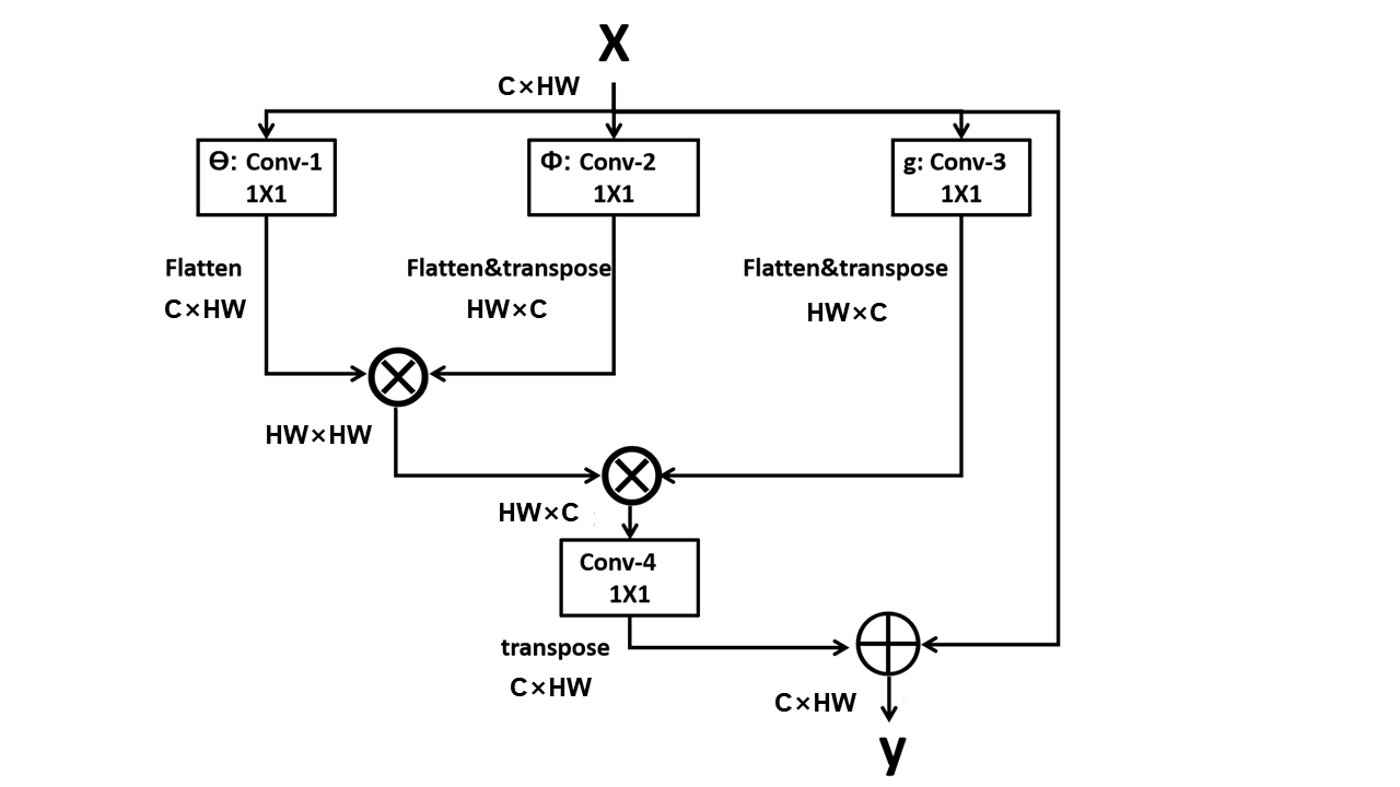
Figure 3. The Nonlocal Block. $\otimes$ and $\oplus$ denote matrix multiplication and element-wise sum. “Conv” denote $1\times 1$ convolution layers. $C$ is the number of channel, $H$ and $W$ are height and width of input feature.

5.3. Feature-Extractor

At each timestamp, Feature-Extractor (i.e., speech spectrogram embedding extraction block) takes a $500$ ms speech Mel-spectrogram as input (section 4.2). We introduce a non-local block in the feature-extractor to capture long-range spatial-temporal relations, followed by convolution layers to extract abstract features.

The non-local block encodes the pairwise relations of all possible positions (frequency and time). Additionally, it encodes the unary information, meaning how a position may have its independent impact on all other positions (Yin et al., 2020). The formal definition of non-local operation is:

(4) $$y_{i}=\frac{1}{C(x)}\sum_{\forall j}f(x_{i},x_{j})g(x_{j})$$

Where $x$ and $y$ are the non-local block’s input and output data. The $C(x)$ is the normalization factor. When computing the output at position $i$ ($y_{i}$), we enumerate all possible position $j$ of $x$. $f(x_{i},x_{j})$ represent the pairwise relation between $x$’s position i and j. It can be distance or affinity. Here we use the Embedded Gaussian function as function f:

(5) $$f(x_{i},x_{j})=e^{\theta(x_{i})^{T}\phi(x_{j})}$$

Here, $\theta(x_{i})=W_{\theta}x_{i}$ and $\phi(x_{j})=W_{\phi}x_{j}$ are embeddings of $x_{i}$ and $x_{j}$, $W_{\theta}$ and $W_{\phi}$ are learnable network parameters. In our implementation, $W_{\theta}$ and $W_{\phi}$ are single-convolution-layers with kernel size of $1\times 1$. $\theta(x_{i})^{T}\phi(x_{j})$ is the dot-product similarity. The normalization factor is set as $C(x)=\sum_{\forall j}f(x_{i},x_{j})$. With this equation, the normalization operation is equal to a softmax operation along the dimension j.

The $g(x_{j})$ represent a simple linear embedding of $x_{j}$: $g(x_{j})=W_{g}x_{j}$, where $W_{g}$ is a learnable network parameter. In our implementation, $W_{g}$ is a single-convolution-layer with a kernel size of $1\times 1$.

Fig. 3 shows the structure of the non-local block. The input signal $x$ is feed into three $1\times 1$ convolutions representing function $\theta$, $\phi$ and $g$. Generated embeddings through these functions are flattened to 1-dimension. The output of $\phi:Conv-2$ is transposed and matrix-multiplied with the output of $\theta:Conv-1$, which represents the pairwise computation shown in equation 5. A softmax operation is followed to normalize the score. The output of $g:Conv-3$ is the linear embedding representation of the input. It was transposed and matrix-multiplied with the softmax output. The output of this multiplication represents the unary information, meaning the independent relation of each position with the correlation of all other positions. A $1\times 1$ convolution and transpose are followed, and the output $y$ has the same shape as input $x$. Additionally, the residual connection makes the module an independent block, allows gradient flow during back-propagation, and improves the training efficiency.

Overall Architecture of the Feature-Extractor: At each timestamp $t$, the feature extractor takes 2-dimensional [HW] (dimensions: HW represents the height, width of input feature respectively) spectrogram $x_{t}$ from a $500$ ms speech as input. First, the input was fed into a stacked nonlocal-convolution structure. Each non-local block is followed by a convolution layer with [$3\times 3$] kernels. The input feature will go through $1$ to $4$ nonlocal-convolution structure. Then the feature map goes through $5$ to $12$ convolution layers with [$3\times 3$] kernels. Later, the output of the convolution layers is flattened and represented as a 1D spectrogram embedding at timestamp $t$. In the end, a linear layer with ReLU activation was used to map the embedding into the desired size.

5.4. Reference-Extractor

Change-score features are 1-dimensional $[1\times 8]$. Reference-extractor block comprises a pair of non-linear layers that take the change-scores as input and generates a 1D physiological feature embedding at each timestamp $t$.

5.5. Overall Architecture: Bi-directional Hyper-LSTM structure

LSTM analyzes information from past to future sequentially and determines a timestamp $t$’s input importance based only on the past information. Bi-directional LSTM (Bi-LSTM) overcomes this limitation by adding a backward LSTM, enabling both past and future context to determine a timestamp $t$’s input importance; thus, achieves better performance (Siami-Namini et al., 2019). Therefore the PASAD implementation uses a bi-directional Hyper-LSTM network (shown in Fig. 2(a)).

The bi-directional Hyper-LSTM network is composed of a forward Hyper-LSTM and a backward Hyper-LSTM. They have the same structure as described in section 5.2. The feature of forward and backward Hyper-LSTM is then concatenated and fed into a CWS vs. CWNS inference generator classifier that is composed of some linear layers with relu activation.

6. Classification Approach Evaluation

This section discusses our evaluations of the PASAD approach on differentiating fluent speech of CWS vs. CWNS from stress-speech and narrative-speech datasets.

Implementation: PASAD approach has four components discussed below. The specific number of layers and number of neurons was set as hyper-parameter and optimized by a python toolkit ”Optuna” (Akiba et al., 2019). It uses a Bayesian Optimization algorithm called Tree-Structured Parzen estimator to identify the optimum set of values. The detailed specifications are provided in the Appendix B.

• The Hyper-LSTM unit comprises of a one-layer auxiliary $LSTM_{aux}$ that generates a 1-dimensional hidden state $\hat{h}_{t}$. We use linear projection (i.e., one-linear layer) to map $\hat{h}_{t}$ to the embedding vectors unique to each gate: $z^{y}_{h}$,$z^{y}_{x}$ and $z^{y}_{b}$ where $y\in\{i,g,f,o\}$. Each of the four gate weights is generated with $z$ and a trainable parameter $W$ following equation $2$ in the main paper. During optimization, we set the number of neurons in $LSTM_{Aux}$ and $LSTM_{main}$ range from 200 to 800 and 600 to 1200 separately. And the dimension of the weight-generating embedding vector ranges from 200 to 800.

• The Feature-Extractor network comprises $1$ to $4$ non-local block and each followed by a convolution layer. There are also $5$ to $12$ convolution layers and 2 linear layers after those non-local blocks with ReLU activation. Batch normalization are used after each convolution layer. During optimization, we set the dimension of embedding range from 200 to 800, and the channel of convolutional layers ranges from 8 to 128.

• The Reference-Extractor are two linear layers with ReLU activation for the stress-speech and narrative-speech dataset implementations. The dimensions of linear layers range from 200 to 800.

• The output of forward and backward Hyper-LSTM are fed into an inference generator classification network. The classification networks comprise three linear layers with dropout and ReLU activations for both the stress-speech and narrative-speech dataset implementations. The number of neurons in linear layers ranges from 600 to 1200.

Baseline Implementations: Following the state-of-the-art works, we considered the CNN-LSTM(Hochreiter and Schmidhuber, 1997), Resnet-9 (Li et al., 2016), Bi-directional LSTM networks(Chen et al., 2017), TDNN (Sheikh et al., 2021), and transformer(Vaswani et al., 2017) as baseline classifiers. For each network, we considered both multi-modal and speech classifiers taking spectrogram and change-score features and only spectrogram as input. The network implementations and configurations are discussed in detail in Appendix A. Classifier-implementations will be made public.

Dataset Split and Evaluation Metrics: For each of the evaluations, we followed the person-disjoint hold-out method (Cawley and Talbot, 2010). Both datasets contain data from different children. We perform 10-fold-cross-validation on both datasets. For each fold, We randomly separate each dataset into person-disjoint test ($4$ children: $2$ CWS, $2$ CWNS), validation ($8$ children: $4$ CWS, $4$ CWNS), and training (the rest of the children) subsets to avoid personal bias and make the models generalizable. Every subset only contains data from some specific individuals, and one child’s data won’t appear in two subsets. This separation is performed randomly ten times; hence we have ten groups of person-disjoint training, validation, and test subset combinations. The presented results are averaged over the ten groups to reduce contingency and avoid overfitting the model. Evaluation results are presented with the metrics: sensitivity, specificity (Swift et al., 2020), accuracy, and F1-score.

In the following sections, we exhaustively evaluated PASAD’s performance (section 6.1), presented Hyper-LSTM unit’s expressiveness and adaptivity to the changes in speech and psychophysiology (section 6.5), demonstrated that PASAD utilizes only speech information in the class inference generation (section 6.6), demonstrated PASAD’s generalizability on unseen age and sex groups (section 6.7), and real-time executability on smart phone and scalable devices (section 6.8).

6.1. Classification Performance

This section discusses models’ performance, ablation evaluation of the PASAD, and comparison of using raw physiological and acoustic features in both datasets.

Models’ Performance. As shown in Table 2, PASAD achieves a relatively higher F1-score of $0.83$ in the stress-speech dataset than the narrative-speech dataset ($0.78$ F1-score). Children experienced higher arousal during the stress-speech task (avg. EDA change-score was 4 times higher), which may result in lesser stable speech construction by the CWS (Tumanova et al., 2020b), hence making the classification task easier in the stress-speech dataset. Moreover, a sentence (i.e., BBAP phrase) was repeated in the stress-speech dataset. A classifier could easily learn the acoustic characteristics of the BBAP phrase from CWS vs. CWNS, which was not the case in the narrative-speech dataset. Hence, PASAD performs relatively higher in the stress-speech dataset.

Tables 2 and 2 show the evaluations of multi-modal and speech baselines, all of which PASAD outperforms. The best-baseline, Transformer, is a temporal-pattern-extracting sequential classifier that further justifies PASAD’s sequential network structure. Additionally, the TDNN’s F1 scores are lower than other baselines. The fact that TDNN uses a time delay structure instead of a sequential model confirms the importance of sequential network structure.

Moreover, the speech baselines have relatively lower efficacy than the multi-modal baselines. It indicates that even experiencing similar situations, CWS and CWNS show distinctive physiological response patterns that multi-modal classifiers can leverage to achieve higher performance.

There is an exception that Resnet-9 achieves lower performance with multi-modal variation in the narrative-speech dataset. The reason is that the model gets overfitted due to the utilization of a large number of trainable parameters to generate input embeddings.

Dataset	Model	Sensitivity	Specificity	Accuracy	F1 score
Stress Speech	PASAD	0.8742	0.7526	81.73%	0.8358
	CNN-LSTM	0.9294	0.4111	68.67%	0.7593
	Resnet-9	0.7822	0.6794	73.4%	0.7578
	TDNN	0.776	0.6515	71.77%	0.7452
	Bi-LSTM	0.7760	0.8048	78.95%	0.7968
	transformer	0.7883	0.8153	80.09%	0.8081
Narrative Speech	PASAD	0.7683	0.837	80.46%	0.7878
	CNN-LSTM	0.7306	0.6961	71.24%	0.7058
	Resnet-9	0.6722	0.7723	72.51%	0.6979
	TDNN	0.6168	0.6722	64.6%	0.622
	Bi-LSTM	0.696	0.8441	77.41%	0.7443
	transformer	0.6861	0.8689	78.26%	0.7487

Table 1. PASAD’s classification performance compared with multi-modal baselines.

Dataset	Model	Sensitivity	Specificity	Accuracy	F1 score
Stress Speech	CNN-LSTM	0.7607	0.6062	68.84%	0.7219
	Resnet-9	0.8742	0.3832	64.43%	0.7233
	TDNN	0.6687	0.6271	64.92%	0.6697
	Bi-LSTM	0.7453	0.5679	66.23%	0.7012
	transformer	0.8312	0.6027	72.43%	0.7623
Narrative Speech	CNN-LSTM	0.6613	0.7909	72.97%	0.698
	Resnet-9	0.6504	0.8697	76.62%	0.7243
	TDNN	0.5564	0.6465	60.4%	0.5702
	Bi-LSTM	0.6089	0.8786	75.12%	0.698
	transformer	0.6504	0.8715	76.71%	0.7251

Table 2. Speech classification baselines’ (only spectrogram as input) performance.

It is important to note that this paper’s classification objective is challenging since both CWS and CWNS are fluently speaking and experiencing similar situations; hence, the situational physiological response differences are subtle and not perceptually differentiable. The evaluation results demonstrate that PASAD effectively extracts CWS vs. CWNS differentiating speech acoustic aspects by leveraging the physiological parameters. In contrast, the baseline multi-modal models concatenate the embeddings extracted from speech and physiological information, and since their (i.e., modalities in CWS vs. CWNS) differences are subtle, the conventional approaches fail to extract similarly effective CWS vs. CWNS differentiating aspects, hence perform relatively poorly than PASAD. The differences in performances are higher in free-speech dataset, due to the relatively more subtle difference in speech and physiological response between CWS and CWNS (discussed above).

6.2. Ablation Study.

Table 4 shows the ablation evaluation where different components of PASAD are modified while keeping the rest of the network the same. The evaluation results and observations are discussed below:

• Non-local Block in Feature-Extractor: Using conventional convolution layers instead of non-local reduces F1-scores $2-3$ percentage points. It indicates that the Non-local block effectively captures the long-range spatial-temporal relations of different frequencies and time, leading to higher performance.

• Only Spectrogram or Change-score Embedding in the $LSTM_{aux}$: Existing studies (Ha et al., 2016; Gui et al., 2018) utilizing HyperNetwork structures put same input in the main $LSTM_{main}$ and auxiliary $LSTM_{aux}$. We aim to classify using speech information; hence the $LSTM_{main}$ takes only spectrogram as input, whereas the $LSTM_{aux}$ extracts physiological response aided temporal speech importance taking both spectrogram and change-score as input. Without the physiological information (i.e., change-score) in $LSTM_{aux}$, PASAD achieves only $0.67$ and $0.76$ F1-scores in stress-speech and narrative-speech datasets, indicating the change-score feature’s efficacy in extracting CWS vs. CWNS differentiating temporal speech information. Using only change-score in the $LSTM_{aux}$, PASAD achieves $0.73$ F1-scores, indicating the effectiveness of the presented PASAD implementation.

Dataset	Modification	Sensitivity	Specificity	Accuracy	F1 score
	PASAD	0.8742	0.7526	81.73%	0.8358
	without non-local block	0.8435	0.7317	79.11%	0.8112
	With only Spectrogram embedding in $LSTM_{aux}$	0.7085	0.5435	63.13%	0.6715
Stress Speech	With only Change-score embedding in $LSTM_{aux}$	0.7208	0.7317	72.59%	0.7366
	PASAD	0.7683	0.837	80.46%	0.7878
	without non-local block	0.7237	0.8724	80.22%	0.7755
	With only Spectrogram embedding in $LSTM_{aux}$	0.7624	0.7839	77.37%	0.7609
Narrative Speech	With only Change-score embedding in $LSTM_{aux}$	0.6822	0.8512	77.14%	0.7381

Table 3. Result for ablation evaluation of PASAD model structure

Dataset	Audio Features	Physio. Features	Sensitivity	Specificity	Accuracy	F1 score
Stress Speech	Raw	Change Score	0.75	0.596	67.31%	0.696
	Spectrogram	Raw	0.6923	0.5962	64.42%	0.6606
Narrative Speech	Raw	Change Score	0.733	0.332	50.9%	0.564
	Spectrogram	Raw	0.7254	0.5042	60.2%	0.627

Table 4. Result for Raw audio & physiological features evaluation

6.3. Raw Physiological Features.

Table 4’s evaluation shows the performance while utilizing the raw physiological features as input in the Reference-Extractor. Raw acoustic features are limited by bias due to different individuals’ variable baseline condition physiological parameters. Conforming to that, the classifiers perform poorly utilizing the raw features.

6.4. Raw Acoustic Features.

Table 4’s evaluation shows the performance while utilizing the raw acoustic features as input. Here, 2D CNN was replaced with 1D due to the input dimension. Such a model cannot extract the pairwise and unary relations across frequency and time of speech acoustic; hence performs relatively poorly.

6.5. $LSTM_{main}$ Gate weights Visualization

This section demonstrates the dynamic changes of the $LSTM_{main}$ gate weights (generated by $LSTM_{aux}$) with the changes in physiological and speech information. Fig. 4 visualize the Mel-spectrogram and change-score features alongside the $LSTM_{main}$ weights changes for two examples. Euclidean distance between the $LSTM_{main}$ weight matrix of the previous and current timestamp is used to compute the gate weights changes.

In the narrative-speech example, HR fluctuates in $1.5$-$3$ & $4$-$4.7$ sec; hence the gate weights have greater changes. In the stress-speech example, participant’s utterance comprises 3 sec; hence $0$-$1$ & $4$-$5$ sec in the spectrogram are zero-padded. Gate weights change significantly in $1$ & $4$ sec, where the zero-pad and speech transition occurs. During $2$-$3$ & $4$-$5$ sec, the HR is rapidly changing, which causes greater changes in the gate weights. The discussion demonstrates that $LSTM_{main}$ gate weights are expressive and adaptive to the speech and change-score information changes.

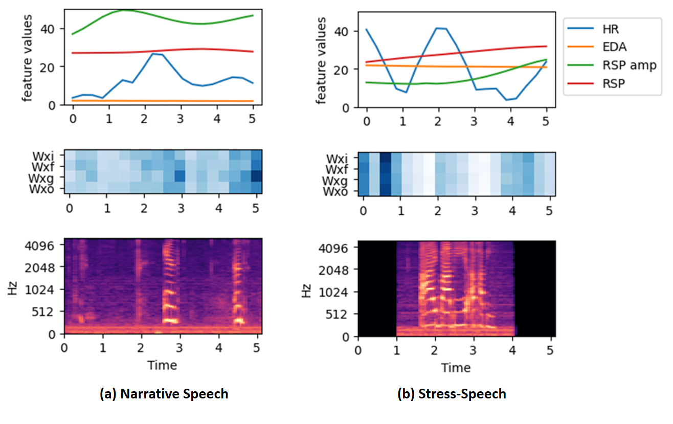
Figure 4. $LSTM_{main}$ Gate weight visualization with respective change-score features and Mel-spectrogram. The time metric is on seconds, and the darkness of the blue color shows gate weight change intensity.

6.6. Data Leakage through Physiological Parameters

Though the weights of $LSTM_{main}$ are adaptive to the speaker’s physiological responses, $LSTM_{main}$ performs classification using only the extracted Mel-spectrogram embeddings. Information leakage through physiological parameters is a concern, meaning if the $LSTM_{main}$ learns CWS vs. CWNS differentiating patterns independently from the change-score features (through the generated weights).

To investigate, we train and evaluate the PASAD approach while replacing the Mel-spectrograms with random noise (on similar frequency ranges) and keeping the actual change-score features. Such classifiers must learn CWS vs. CWNS differentiating patterns independently from the change-score feature. The evaluation is shown in table 5, where the classifiers perform significantly poorly (i.e., random inferences), demonstrating the absence of information/data leakage.

Dataset	Sensitivity	Specificity	Accuracy	F1 score
Stress-Speech	0.6346	0.5	56.73%	0.5946
Narrative-Speech	0.3208	0.5212	43.26%	0.3348

Table 5. Evaluation of PASAD by replacing Mel-spectrograms with random noise

6.7. Age and Sex -Wise Analyze

This section discusses PASAD’s efficacy in different sex and age groups. For a fair comparison, we perform this section’s evaluation on the stress-speech dataset where all participants uttered the same ‘Buy Bobby a puppy,’ i.e., BBAP phrase experiencing the same condition.

Notably, in the stress-speech dataset, 9 children (2 female, 7 male) were 3-4 years of age, 16 children (3 female, 13 male) were 4-5 years of age, and 13 (all male) were over 5 years of age. The evaluation results are shown in Table 6. The relatively poor performance in the female group is due to the imbalanced male vs. female ratio in the dataset. It is in line with the general population since stuttering is more common among males (Craig et al., 2002; Yairi and Ambrose, 2004). However, PASAD achieves higher performance in the higher age group. Previous literature (Green et al., 2000) showed that SMCs are unstable in smaller age groups irrespective of whether they stutter or not. Hence, differentiating fluent speech of CWS vs. CWNS in the small age groups is difficult. With higher age, the SMC gets more stable; hence it is easier to identify the CWS indicative SMC instabilities in the higher age groups. Hence, PASAD’s performance is in line with the literature.

Importantly, this section’s evaluation demonstrates that PASAD generalizes and performs relatively uniformly in each age-sex group.

Sex	3-4 years old	4-5 years old	over 5 years old	Average
Female	100%	76.49%	0	88.24%
Male	80.39%	90.68%	93.09%	89.42%
Average	85.29%	88.5%	93.09%

Table 6. Average accuracy sex-wise and age-wise in stress-speech dataset

6.8. Execution Time and Resource Usage

To evaluate the PASAD’s real-time executability and resource usage, we deploy the approach on an Nvidia Jetson Nano (jet, 2022) and smart phone(pix, 2022). The jetson nano is equipped with NVIDIA Maxwell GPU, Quad-core ARM processor, and 4GB memory. The smart phone is Google Pixel 6 with 8gb ram and eight cores CPU. We run the models taking consecutive $5$ sec windows for $10$ minutes ($120$ repetitions) and record the running time and resource usage. As shown in table 7, both models take about 1 sec to process a $5$ sec speech information on both jetson nano and smartphone. The average CPU and GPU usages are $15$-$16$% and $8$-$12$% on jetson nano. And the average CPU usage on smart phone is $3$2%-$33$%. On the jetson nano, the average RAM usage is around 2.4Gb. For the smartphone execution, we optimize the model for mobile execution, and the RAM usage is as low as around 0.33Gb; hence, the models do not significantly occupy the resource. The results suggest that PASAD can perform real-time analysis on resource-constraint devices.

Model	stress speech model (jetson nano)	narrative speech model (jetson nano)	stress speech model (smartphone)	narrative speech model (smartphone)
Running time	0.8966 s	1.0237 s	0.580 s	1.67 s
Average CPU usage	15.06%	15.87%	32%	33%
Average GPU usage	8.59%	11.87%	N/A	N/A
Average RAM usage	2.4Gb/4Gb	2.5Gb/4Gb	0.33Gb/8Gb	0.35Mb/8Gb

Table 7. Average running time and resource usage

7. PASAD Model Interpretation Discussion

This section demonstrates how PASAD’s inferences can be utilized to understand stuttering children’s speech and SMC differences from the others. Understanding which Mel-spectrogram frequencies across time are important for each of the PASAD’s inference generation is critical since they contribute most to differentiating a CWS’s respective speech from others. We employ Kernel SHAP, a model-agnostic interpretation framework, that leverages PASAD’s HyperNetwork architecture to identify the critical Mel-spectrogram frequencies that $LSTM_{main}$ utilizes for CWS vs. CWNS inference generation. The following sections discuss the Kernel SHAP employment procedure, how different Mel-spectrogram frequencies (e.g., formants, $F0$) refer to the deviation in different speech-motor-control components (i.e., articulators) and demonstrate important distinct information identification from CWS’s fluent speech through the PASAD’s inference interpretation visualization.

7.1. PASAD’s Kernel SHAP Employment Procedure

Kernel SHAP approximates the conditional expectations of Shapley values in deep learning models by perturbing the input (i.e., different portions/attributes of input) and observing the impact on the output (Lundberg and Lee, 2017). Shapley values (Shapley, 1953) correspond to the contribution of each input portion towards pushing the model inference closer or away from the true class value. The kernel SHAP trains a surrogate weighted linear regression model based on artificial samples generated by perturbing the input (of which we are generating interpretation) and the original deep learning model’s inferences on those perturbed samples (Rodríguez-Pérez and Bajorath, 2020). Then use the coefficients of the linear regression model to determine the input feature (i.e., attributes) importance.

However, we cannot directly employ the Kernal SHAP in our PASAD model. PASAD takes both Mel-spectrogram and change-score physiological information as input, and kernel SHAP’s linear regression model trained on such combined input would not be able to differentiate the independent impact of the Mel-spectrogram from change-score information. Notably, we are only interested in interpreting the Mel-spectrogram information’s impact on PASAD’s inferences (that $LSTM_{main}$ uses for inference generation). The change score psychophysiology data is only for reference (generating weights of $LSTM_{main}$), meaning we need to exclude the auxiliary network $LSTM_{aux}$ when applying the kernel SHAP.

The unique structure of PASAD enables us to address the challenge and extract the independent importance of Mel-spectrogram information in PASAD’s inference generation. In the presented PASAD model, the change-score psychophysiology data is only for generating the weight of $LSTM_{main}$. The $LSTM_{aux}$ takes the spectrogram and psychophysiology embeddings to generate the gate weights of $LSTM_{main}$. The $LSTM_{main}$ takes only the spectrogram’s embedding and makes the inference. Therefore, as the first stage of interpretation generation, we run the complete PASAD model with unperturbed original Mel-spectrogram (of which we are generating interpretation) and change-score input and save the gate weights of $LSTM_{main}$. Later, in the second stage, Kernel SHAP is applied to the feature-extractor and $LSTM_{main}$ (with already learned gate-weights); where Kernel SHAP retrieves inferences of perturbed samples (of the original Mel-spectrogram), train linear regression model based on that, and generate the importance of different attributes of the original Mel-spectrogram.

Notably, we are interested in generating the importance of different Mel-spectrogram frequencies (i.e., attributes). Hence, we divide the Mel-spectrogram into 32 frequency bands and use these bands as tokens for the Kernel SHAP. While generating the perturbation of the original Mel-spectrogram, we permute the tokens, meaning we replace all pixels within the frequency band with the background/other data and feed it into the kernel SHAP. After the Kernel SHAP analysis, each frequency band was assigned a Shapley (SHAP) value to represent its contribution to prediction. Finally, we visualize them with a horizontal bar plot. The following sections discuss how different Mel-spectrogram frequencies (e.g., formants, $F0$) refer to the deviation in different SMC components and demonstrate important distinct information identification from CWS’s fluent speech through the PASAD’s inference interpretation visualization.

7.2. Mel-spectrogram Frequency Attributes and Speech-motor-control(SMC)

As discussed in section 4.2.1, Formants are the peak points (i.e., bands running horizontally across the spectrogram) of the amplitude in the spectrogram. They change with changes in the vocal tract configuration as speakers move their articulators (jaw, tongue) to produce a specific sound. Existing literature (Vorperian et al., 2019) evaluated the lowest four formants ($F1$-$F4$) in distinguishing unique vowel sounds. $F1$ & $F2$ are associated with the position of the tongue. The height of the tongue in the mouth is inversely related to $F1$, such that high vowels have lower $F1$ values and vice versa. The $F2$ is directly related to tongue advancement (how far back the tongue is in the mouth). Back vowels have lower $F2$ values and vice versa. $F3$ (Lindblom et al., 1979) is associated with the front cavity formed by the lips and the tongue constriction, and $F4$ (Vorperian et al., 2019) is associated with laryngeal descent/elevation and the pharyngeal and hypopharyngeal cavities. Additionally, lower SMC is positively correlated with higher fundamental frequency $F0$ variability (Robb and Saxman, 1985). Also, deviation in high frequency indicates deviation to aerodynamic and resonance properties in the vocal tract (i.e., tongue placement) (Denny and Smith, 2000).

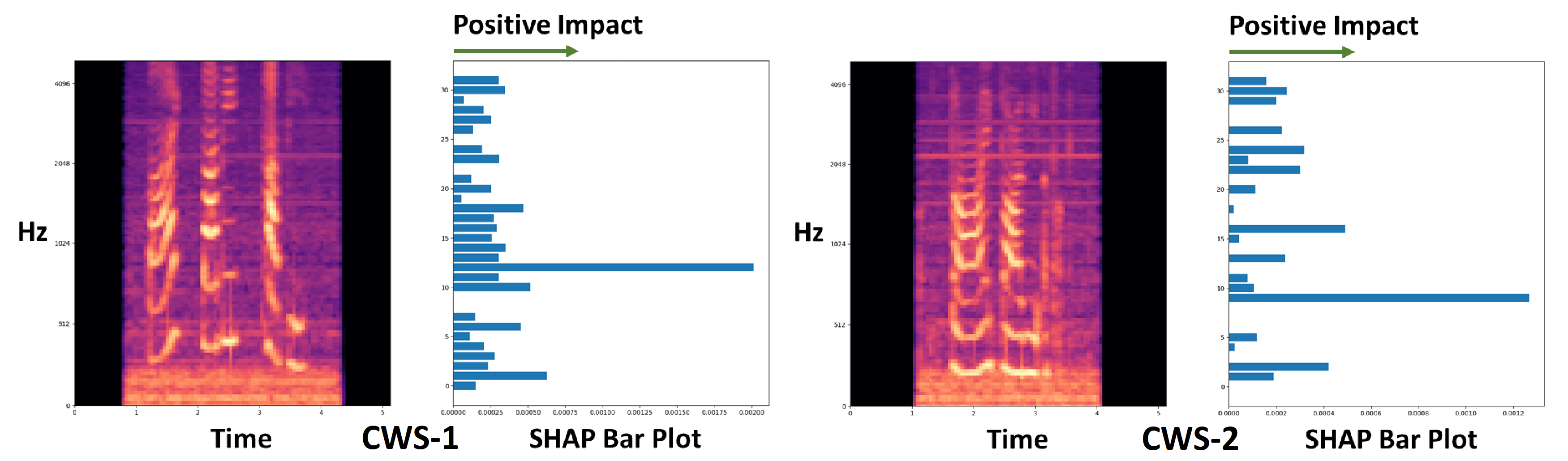
(a) CWS samples from stress-speech dataset

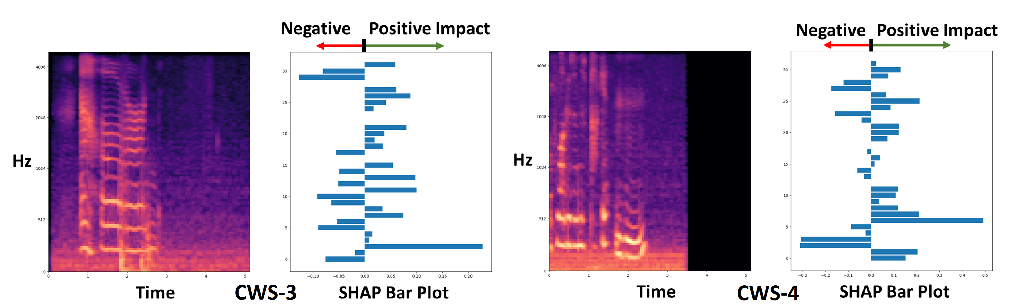
(b) CWS samples from narrative-speech dataset

Figure 5. Visualization of important spectrogram coordinates for CWS speech samples

7.3. Interpretation Discussion

Fig. 5(a) and 5(b) show the PASAD model Shapley interpretation of different CWS participants’ speech. In each figure, the left-side is the Mel-spectrogram, and the right-side is the Shapley importance bar-plot for different frequencies.

According to Fig. 5(a), both CWS participants’ BBAP phrase speech have higher $F0$ (0-300Hz) variability indicating lower SMC and higher physiological arousal. It is in line since they are experiencing higher arousal during this stress-speaking task. Moreover, the Shapley importance is higher for $F3$, indicating deviation in their cavity formation by the lip and tongue constriction.

According to Fig. 5(b), the $F1$ has higher Shapley importance for both CWS participants from the narrative-speech dataset. It indicates that they have deviations in tongue positions while speaking vowels. Participant CWS-3 has higher Shapley values associated with $F4$, indicating deviation associated with laryngeal descent/elevation and the pharyngeal and hypopharyngeal cavities. Participants CWS-4 has higher Shapley values associated with $F3$, indicating deviations in cavity formation by lip and tongue constriction. Both participants have relatively higher Shapley values in higher frequencies, indicating minor deviation in tongue placement.

This section demonstrates that the presented approach can identify important SMC (and corresponding speech articulator) information from CWS’s fluent speech, making it impactful for practical use.

8. Discussion and Broader Impact

This section discusses some key observations, broader impact, and limitations of the study:

Novelty in Capturing the Dynamic Nature of Speech: PASAD’s novelty is its unique adaptation of physiological information to analyze speech information dynamically. PASAD’s HyperNetwork enables such adaptivity. The auxiliary network (i.e., $LSTM_{aux}$) takes physiological and audio information to measure momentary/situational arousal and generates the main network’s (i.e., $LSTM_{main}$) weight accordingly. The main network makes inferences taking only audio information as input, and its weights are equivalent to the rules/processing applied to the audio features. Since the main network’s weights change with arousal changes, PASAD is the first-of-its-kind way of audio (one modality) processing where processing rules are adaptive to the changes in physiological arousal responses (different modality). As common in the clinical domain, our dataset is limited (still one of the largest datasets on stuttering children); hence a simple LSTM network implementation was utilized. But the presented unique way of dynamically analyzing one modality while being adaptive to different modalities is transferrable to other domains and more complex network architectures.

Model Interpretation Generation: PASAD’s unique architecture enables identifying the contribution of speech attributes in differentiating CWS vs. CWNS. Evaluation in section 6.6 establishes that only speech information is utilized by the inference generating $LSTM_{main}$ network, and it does not learn CWS vs. CWNS differentiating patterns independently from the physiological parameters (i.e., change-score feature). Hence, during model interpretation generation (section 7), applying Kernel SHAP on the pre- gate-weight-computed $LSTM_{main}$ identifies the contribution of Mel-spectrogram frequencies toward generated inferences.

Discussion on Dataset Task Conditions: Existing speech science studies (Byrd et al., 2012; Tumanova et al., 2020b) use structured tasks that can effectively elicit specific behavior-related data from the stuttering individuals in which clinicians are interested. Particularly, speaking in stress conditions (Clark et al., 2012; Guttormsen et al., 2015; Vanryckeghem et al., 2005) and narration tasks (Weiss and Zebrowski, 1994; Zackheim and Conture, 2003) are of interest due to the elicitation of arousal due to external stressors and cognitive loads. Following the existing studies, PASAD identifies and visualizes the fluent speech attributes that distinguish CWS vs. CWNS in these two conditions.

Broader Impact and Application of PASAD: It is important to note that speech-science studies (Bauerly, 2018; Robb et al., 1998) and clinicians also leverage the stuttering individuals’ speech spectrograms to identify important formants, frequencies, and their corresponding SMC components through manual observations. As discussed in section 7.3, PASAD enables automated identification of such information from each $5$ sec speech. Additionally, the collected Dataset’s sensing modalities are present in recent wearables. For example, same Biopac sensors utilized in this study (section 3) are present in Biopac wireless wearable system (bio, 2022)); hence PASAD can be implemented and evaluated in wearables. According to our evaluation in section 6.8, PASAD is real-time executable in smart devices (e.g., smartphones). Hence, PASAD has the potential to be leveraged for remote, continuous, automated, and real-time assessment of stuttering children’s fluent-speech and SMC deviation.

Furthermore, speech scientists would be able to leverage PASAD to enhance their understanding of CWS’s SMC and speech deviations. However, such analysis is out of the scope of this paper.

Study Limitations: The study’s limitation is that we analyzed data from only two conditions. Future work would benefit from sampling data from a wider range of situations to determine the boundaries of the models’ predictive validity. Additionally, in the future, PASAD can be implemented and evaluated on wearables for the longitudinal understanding of CWS’s speech characteristics.

9. Conclusion

The presented approach effectively identifies and visualizes the speech Mel-spectrogram pattern differences in preschool-age CWS and CWNS while speaking perceptually fluently in two challenging conditions: speaking in stressful situations and narration. To our knowledge, PASAD is the first approach that leveraged the HyperNetwork structure on multi-modal sensing data. PASAD utilizes the speaker’s physiological response for effective acoustic analysis and makes classification decisions using only speech information; ergo, it is not a multi-modal sensor data integration approach but a speech analysis approach that is adaptive to the speaker’s situational physiological arousal. For a comprehensive comparison, this paper compares PASAD with multiple multi-modal classifiers and speech classifiers, all of which PASAD outperforms. Its high efficacy establishes that CWS’s distinct speech-motor-control is dynamic in nature and conforms to the respective speaker’s situational emotional reactivity. Our comprehensive evaluation of multiple speech conditions, ablation evaluation, and several baselines establish PASAD’s efficacy, expressiveness, and generalizability. Finally, the presented interpretation discussion in section 7.3 shows the PASAD’s feasibility in understanding CWS’s SMC deviations and corresponding speech articulators, making PASAD highly impactful for practical use.

Appendix:

Appendix A Baseline Network Implementations

In the multi-modal evaluations, the CNN-LSTM model comprises a spectrogram embedding extractor block consisting of $3$ to $5$ convolution layer followed by $2$ linear layers, a change-score embedding extractor block comprises of two linear layers, a single-layered LSTM, and a classifier comprises of two linear layers. The spectrogram and physiological features go through the spectrogram and change-score embedding extractor block, respectively. Then their embedding was concatenated and feeds into a single-layer LSTM. The classifier takes the last hidden state of LSTM as input and makes a classification. All linear and convolution layers used the ReLU activation function. Each convolution layer is followed by batch normalization.

The Resnet-9, bidirectional LSTM, and transformer share a similar structure as the CNN-LSTM. The ResNet-9 replaces the convolution layers in the spectrogram embedding extractor with residual network layers. The bidirectional LSTM and transformer replace single-layered LSTM with bidirectional LSTM and transformer encoder, respectively.

The Time delay neural network(TDNN) model has been shown to efficiently model long-term temporal dependencies between acoustic events. Different from other baseline models, the spectrogram embedding extractor block of TDNN baseline takes the 5s window spectrogram as input and generates the spectrogram embedding. The physiological features go through the change-score embedding extractor block and a single-layered LSTM. Then Concatenate with the spectrogram embedding and feed into the classifier for prediction.

To further evaluate the multi-modal baseline, we try concatenate the embeddings after the sequential model. The basic idea is to process the spectrogram and physiological embeddings with a separate sequential model(LSTM or transformer), and then concatenate for prediction. The embedding of spectrogram and physiological features was fed into separate LSTMs or Transformers and then concatenated. The classifier takes the concatenated feature as input and make the prediction. The configurations of the spectrogram embedding extractor, change-score embedding extractor, and classifier are the same as other baselines. For each baseline, we try both concatenate embeddings before and after the sequential model. Then only take the best result among the two varations. In CNN-LSTM, Bi-LSTM, and transformer baseline, concatenate embeddings after the sequential model achieve better performance. In contrast, the Resnet-9 achieves better performance with concatenating embeddings before the sequential model.

In the speech classifier evaluations, the baseline models take only spectrograms as input. The spectrogram feature goes through the spectrogram embedding extractor block, sequential model, and classifier. The embedding extractor block, sequential model, and classifier followed the same configuration as the multi-modal does.

The specific number of layers and number of neural were set as hyper-parameter. All the network configurations and hyper-parameters were identified through the python toolkit Optuna (Akiba et al., 2019). It uses a Bayesian Optimization algorithm called the Tree-Structured Parzen estimator to identify the optimum set of values.

Appendix B Configurations

System Configuration All evaluations are carried out in a distributed computing system comprising 14,000 cores and 20 terabytes of memory. The system is optimized to perform a large number of smaller parallel jobs. We submit the program as a job, and each job will be assigned 2 CPUs and a GPU. The GPU was randomly selected from a resource pool including NVIDIA RTX A6000, NVIDIA RTX 6000, NVIDIA RTX 5000, NVIDIA GeForce GTX 1080 Ti, and NVIDIA GeForce GTX 750 Ti.

Training Configuration We perform 10 fold-cross validation on both stress-speech and narrative-speech datasets And run Optuna for each test subset independently. To ensure reproducibility, we set the random seed as 2021 for the stress-speech task and 2022 for the narrative-speech task. We also set the PyTorch using deterministic algorithms to limit the number of sources of nondeterministic behavior. During training, we try the learning rate range from 1e-6 to 1e-4. The drop-out rate of linear layers ranges from 0.1 to 0.3. The batch size range from 5 to 10.

Finalized hyper-parameters Here, we present examples of finalized hyper-parameters of PASAD model for stress-speech task and narrative-speech task. In the stress-speech dataset, we achieve the best performance with the following parameters: the dimension of spectrogram embedding is 533, the number of the channels of convolutional layers is 62, the number of convolutional layers is 7, the number of the non-local block is 1, the dimension of reference embedding is 506, the number of neurons of $LSTM_{aux}$ and $LSTM_{main}$ is 234 and 915, the dimension of weight-generating embedding vector is 487. The learning rate is 6.979e-05, the drop-out rate is 0.2915, and the batch size is 10. In the narrative-speech dataset, we achieve the best performance with the following parameters: the dimension of spectrogram embedding is 631, the number of the channels of convolutional layers is 105, the number of convolutional layers is 6, the number of the non-local block is 2, the dimension of reference embedding is 249, the number of neurons of $LSTM_{aux}$ and $LSTM_{main}$ is 378 and 1078, the dimension of weight-generating embedding vector is 715. The learning rate is 2.078e-06, the drop-out rate is 0.2125, and the batch size is 5.

Important Note: The codes, extracted features, and data samples will be made public for reproducibility.

References

- (1)
- bio (2016) 2016. Biopac MP150 hardware system. https://www.biopac.com/wp-content/uploads/MP150-Systems.pdf. Accessed: 2022-05-01.
- bio (2022) 2022. Biopac Wireless Wearable Physiology Sensing system. https://www.biopac.com/product-category/research/bionomadix-wireless-physiology/. Accessed: 2022-05-01.
- pix (2022) 2022. Google pixel 6. https://store.google.com/product/pixel_6. Accessed: 2022-05-15.
- jet (2022) 2022. Jetson Nano Developer Kit. https://developer.nvidia.com/embedded/jetson-nano-developer-kit. Accessed: 2022-05-15.
- shu (2022) 2022. shure sm58 microphone. https://www.shure.com/en-US/products/microphones/sm58. Accessed: 2022-05-01.
- stu (2022) 2022. Stuttering population in USA. https://www.stutteringhelp.org/prevalence. Accessed: 2022-05-01.
- Akiba et al. (2019) Takuya Akiba, Shotaro Sano, Toshihiko Yanase, Takeru Ohta, and Masanori Koyama. 2019. Optuna: A Next-generation Hyperparameter Optimization Framework. arXiv:1907.10902 [cs.LG]
- Amster and Starkweather (1987) Barbara J Amster and C Woodruff Starkweather. 1987. Articulatory rate, stuttering and speech motor control. In Speech motor dynamics in stuttering. Springer, 317–328.
- Arenas and Zebrowski (2013) Richard Arenas and Tricia Zebrowski. 2013. The effects of autonomic arousal on speech production in adults who stutter: A preliminary study. Speech, Language and Hearing 16, 3 (2013), 176–185.
- Banse and Scherer (1996) Rainer Banse and Klaus R Scherer. 1996. Acoustic profiles in vocal emotion expression. Journal of personality and social psychology 70, 3 (1996), 614.
- Bauerly (2018) Kim R Bauerly. 2018. The effects of emotion on second formant frequency fluctuations in adults who stutter. Folia Phoniatrica et Logopaedica 70, 1 (2018), 13–23.
- Bauerly and Bilardello (2021) Kim R Bauerly and Cameron Bilardello. 2021. Resting autonomic activity in adults who stutter and its association with self-reports of social anxiety. Journal of Fluency Disorders 70 (2021), 105881.
- Bauerly et al. (2019) Kim R Bauerly, Robin M Jones, and Charlotte Miller. 2019. Effects of Social Stress on Autonomic, Behavioral, and Acoustic Parameters in Adults Who Stutter. Journal of Speech, Language, and Hearing Research 62, 7 (2019), 2185–2202.
- Benesty et al. (2008) Jacob Benesty, M Mohan Sondhi, and Yiteng Arden Huang. 2008. Introduction to speech processing. In Springer Handbook of Speech Processing. Springer, 1–4.
- Bhattacharya and Shahnawaz (2021) Samayan Bhattacharya and Sk Shahnawaz. 2021. Animal inspired Application of a Variant of Mel Spectrogram for Seismic Data Processing. arXiv preprint arXiv:2109.10733 (2021).
- Bradley and Lang (2007) Margaret M Bradley and Peter J Lang. 2007. Emotion and motivation. (2007).
- Byrd et al. (2012) Courtney T Byrd, Kenneth J Logan, and Ronald B Gillam. 2012. Speech disfluency in school-age children’s conversational and narrative discourse. (2012).
- Carter et al. (2017) Alice Carter, Lauren Breen, J Scott Yaruss, and Janet Beilby. 2017. Self-efficacy and quality of life in adults who stutter. Journal of fluency disorders 54 (2017), 14–23.
- Caruso et al. (1994) Anthony J Caruso, Wojtek J Chodzko-Zajko, Debra A Bidinger, and Ronald K Sommers. 1994. Adults who stutter: Responses to cognitive stress. Journal of Speech, Language, and Hearing Research 37, 4 (1994), 746–754.
- Cawley and Talbot (2010) Gavin C Cawley and Nicola LC Talbot. 2010. On over-fitting in model selection and subsequent selection bias in performance evaluation. The Journal of Machine Learning Research 11 (2010), 2079–2107.
- Chen et al. (2017) Tao Chen, Ruifeng Xu, Yulan He, and Xuan Wang. 2017. Improving sentiment analysis via sentence type classification using BiLSTM-CRF and CNN. Expert Systems with Applications 72 (2017), 221–230.
- Cheng et al. (2016) Jianpeng Cheng, Li Dong, and Mirella Lapata. 2016. Long short-term memory-networks for machine reading. arXiv preprint arXiv:1601.06733 (2016).
- Clark et al. (2012) Chagit E Clark, Edward G Conture, Carl B Frankel, and Tedra A Walden. 2012. Communicative and psychological dimensions of the KiddyCAT. Journal of communication disorders 45, 3 (2012), 223–234.
- Craig et al. (1992) Ashley Craig, Esther Chang, and Karen Hancock. 1992. Treatment success for children who stutter: A critical review. Australian Journal of Human Communication Disorders 20, 1 (1992), 81–92.
- Craig et al. (2002) Ashley Craig, Karen Hancock, Yvonne Tran, Magali Craig, and Karen Peters. 2002. Epidemiology of stuttering in the community across the entire life span. (2002).
- Curlee (1993a) Richard F Curlee. 1993a. The early history of the behavior modification of stuttering: From laboratory to clinic. Journal of fluency disorders (1993).
- Curlee (1993b) Richard F Curlee. 1993b. Evaluating treatment efficacy for adults: Assessment of stuttering disability. Journal of Fluency Disorders 18, 2-3 (1993), 319–331.
- Curlee and Yairi (1997) Richard F Curlee and Ehud Yairi. 1997. Early intervention with early childhood stuttering: A critical examination of the data. American Journal of Speech-Language Pathology 6, 2 (1997), 8–18.
- Deller et al. (2000) John R Deller, John G Proakis, and John HL Hansen. 2000. Discrete-time processing of speech signals. Institute of Electrical and Electronics Engineers.
- Denny and Smith (2000) Margaret Denny and Anne Smith. 2000. Respiratory control in stuttering speakers: Evidence from respiratory high-frequency oscillations. Journal of Speech, Language, and Hearing Research 43, 4 (2000), 1024–1037.
- Diehl et al. (2019) Janine Diehl, Michael P Robb, John G Lewis, and Tika Ormond. 2019. Situational speaking anxiety in adults who stutter. Speech, Language and Hearing 22, 2 (2019), 100–110.
- Dieleman and Schrauwen (2014) Sander Dieleman and Benjamin Schrauwen. 2014. End-to-end learning for music audio. In 2014 IEEE International Conference on Acoustics, Speech and Signal Processing (ICASSP). IEEE, 6964–6968.
- Erdemir et al. (2018) Aysu Erdemir, Tedra A Walden, Caswell M Jefferson, Dahye Choi, and Robin M Jones. 2018. The effect of emotion on articulation rate in persistence and recovery of childhood stuttering. Journal of fluency disorders 56 (2018), 1–17.
- Fuller et al. (1992) Barbara F Fuller, Yoshiyuki Horii, and Douglas A Conner. 1992. Validity and reliability of nonverbal voice measures as indicators of stressor-provoked anxiety. Research in nursing & health 15, 5 (1992), 379–389.
- Gerratt (1983) Bruce R Gerratt. 1983. Formant frequency fluctuation as an index of motor steadiness in the vocal tract. Journal of Speech, Language, and Hearing Research 26, 2 (1983), 297–304.
- Giannakakis et al. (2019) Giorgos Giannakakis, Dimitris Grigoriadis, Katerina Giannakaki, Olympia Simantiraki, Alexandros Roniotis, and Manolis Tsiknakis. 2019. Review on psychological stress detection using biosignals. IEEE Transactions on Affective Computing (2019).
- Green et al. (2000) Jordan R Green, Christopher A Moore, Masahiko Higashikawa, and Roger W Steeve. 2000. The physiologic development of speech motor control: Lip and jaw coordination. Journal of Speech, Language, and Hearing Research 43, 1 (2000), 239–255.
- Gui et al. (2018) Tao Gui, Qi Zhang, Jingjing Gong, Minlong Peng, Di Liang, Keyu Ding, and Xuan-Jing Huang. 2018. Transferring from formal newswire domain with hypernet for twitter pos tagging. In Proceedings of the 2018 Conference on Empirical Methods in Natural Language Processing. 2540–2549.
- Guo et al. (2007) Wu Guo, Renhua Wang, and Lirong Dai. 2007. Mel-Cepstrum integrated with pitch and information of voiced/unvoiced. Shuju Caiji yu Chuli(Journal of Data Acquisition & Processing) 22, 2 (2007), 229–233.
- Guo-an (2011) DAI Guo-an. 2011. Design and Implementation of a Voice Recognition System in Car Alarm. Science and Technology of West China 13 (2011).
- Guttormsen et al. (2015) Linn Stokke Guttormsen, Elaina Kefalianos, and Kari-Anne B Næss. 2015. Communication attitudes in children who stutter: A meta-analytic review. Journal of fluency disorders 46 (2015), 1–14.
- Ha et al. (2016) David Ha, Andrew Dai, and Quoc V Le. 2016. Hypernetworks. arXiv preprint arXiv:1609.09106 (2016).
- Hecker et al. (1968) Michael HL Hecker, Kenneth N Stevens, Gottfried von Bismarck, and Carl E Williams. 1968. Manifestations of task-induced stress in the acoustic speech signal. The Journal of the Acoustical Society of America 44, 4 (1968), 993–1001.
- Heyde et al. (2016) Cornelia J Heyde, James M Scobbie, Robin Lickley, and Eleanor KE Drake. 2016. How fluent is the fluent speech of people who stutter? A new approach to measuring kinematics with ultrasound. Clinical linguistics & phonetics 30, 3-5 (2016), 292–312.
- Hochreiter and Schmidhuber (1997) Sepp Hochreiter and Jürgen Schmidhuber. 1997. Long short-term memory. Neural computation 9, 8 (1997), 1735–1780.
- Howell et al. (2009) Peter Howell, Stephen Davis, and Jon Bartrip. 2009. The university college london archive of stuttered speech (uclass). (2009).
- Jackson et al. (2016) Eric S Jackson, Mark Tiede, Deryk Beal, and Douglas H Whalen. 2016. The impact of social–cognitive stress on speech variability, determinism, and stability in adults who do and do not stutter. Journal of Speech, Language, and Hearing Research 59, 6 (2016), 1295–1314.
- Jones et al. (2014) Robin M Jones, Anthony P Buhr, Edward G Conture, Victoria Tumanova, Tedra A Walden, and Stephen W Porges. 2014. Autonomic nervous system activity of preschool-age children who stutter. Journal of fluency disorders 41 (2014), 12–31.
- Jones et al. (2017) Robin M Jones, Tedra A Walden, Edward G Conture, Aysu Erdemir, Warren E Lambert, and Stephen W Porges. 2017. Executive functions impact the relation between respiratory sinus arrhythmia and frequency of stuttering in young children who do and do not stutter. Journal of Speech, Language, and Hearing Research 60, 8 (2017), 2133–2150.
- Kourkounakis et al. (2020) Tedd Kourkounakis, Amirhossein Hajavi, and Ali Etemad. 2020. Detecting Multiple Speech Disfluencies Using a Deep Residual Network with Bidirectional Long Short-Term Memory. In ICASSP 2020-2020 IEEE International Conference on Acoustics, Speech and Signal Processing (ICASSP). IEEE, 6089–6093.
- Kurniawan et al. (2013) Hindra Kurniawan, Alexandr V Maslov, and Mykola Pechenizkiy. 2013. Stress detection from speech and galvanic skin response signals. In Proceedings of the 26th IEEE International Symposium on Computer-Based Medical Systems. IEEE, 209–214.
- Ladefoged et al. (1978) Peter Ladefoged, Richard Harshman, Louis Goldstein, and Lloyd Rice. 1978. Generating vocal tract shapes from formant frequencies. The Journal of the Acoustical Society of America 64, 4 (1978), 1027–1035.
- Lang et al. (1997) Peter J Lang, Margaret M Bradley, Bruce N Cuthbert, et al. 1997. International affective picture system (IAPS): Technical manual and affective ratings. NIMH Center for the Study of Emotion and Attention 1, 39-58 (1997), 3.
- Li et al. (2016) Sihan Li, Jiantao Jiao, Yanjun Han, and Tsachy Weissman. 2016. Demystifying resnet. arXiv preprint arXiv:1611.01186 (2016).
- Lindblom et al. (1979) Björn Lindblom, James Lubker, and Thomas Gay. 1979. Formant frequencies of some fixed-mandible vowels and a model of speech motor programming by predictive simulation. Journal of Phonetics 7, 2 (1979), 147–161.
- Lu et al. (2018) Guanming Lu, Liang Yuan, Wenjuan Yang, Jingjie Yan, and Haibo Li. 2018. Speech emotion recognition based on long short-term memory and convolutional neural networks. Journal of Nanjing University of Posts and Telecommunications 38, 5 (2018), 63–69.
- Lundberg and Lee (2017) Scott M Lundberg and Su-In Lee. 2017. A unified approach to interpreting model predictions. In Advances in neural information processing systems. 4765–4774.
- Mayer (1974) Mercer Mayer. 1974. Frog goes to dinner. (1974).
- Mermelstein (1967) Paul Mermelstein. 1967. Determination of the vocal-tract shape from measured formant frequencies. The Journal of the Acoustical Society of America 41, 5 (1967), 1283–1294.
- Natke and Kalveram (2001) Ulrich Natke and Karl Theodor Kalveram. 2001. Fundamental frequency and vowel duration under frequency shifted auditory feedback in stuttering and nonstuttering adults. In Fluency disorders: Theory, research, treatment and selfhelp. Proceedings of the Third World Congress on Fluency Disorders in Nyborg, Denmark. Citeseer, 66–71.
- Partila et al. (2015) Pavol Partila, Miroslav Voznak, and Jaromir Tovarek. 2015. Pattern recognition methods and features selection for speech emotion recognition system. The Scientific World Journal 2015 (2015).
- Protopapas and Lieberman (1997) Athanassios Protopapas and Philip Lieberman. 1997. Fundamental frequency of phonation and perceived emotional stress. The Journal of the Acoustical Society of America 101, 4 (1997), 2267–2277.
- Ravikumar et al. (2009) KM Ravikumar, R Rajagopal, and HC Nagaraj. 2009. An approach for objective assessment of stuttered speech using MFCC. In The international congress for global science and technology. 19.
- Ravikumar et al. (2008) KM Ravikumar, Balakrishna Reddy, R Rajagopal, and H Nagaraj. 2008. Automatic detection of syllable repetition in read speech for objective assessment of stuttered disfluencies. Proceedings of world academy science, engineering and technology 36 (2008), 270–273.
- Robb et al. (1998) Michael Robb, Michael Blomgren, and Yang Chen. 1998. Formant frequency fluctuation in stuttering and nonstuttering adults. Journal of fluency disorders 23, 1 (1998), 73–84.
- Robb and Saxman (1985) Michael P Robb and John H Saxman. 1985. Developmental trends in vocal fundamental frequency of young children. Journal of Speech, Language, and Hearing Research 28, 3 (1985), 421–427.
- Rodríguez-Pérez and Bajorath (2020) Raquel Rodríguez-Pérez and Jürgen Bajorath. 2020. Interpretation of machine learning models using shapley values: application to compound potency and multi-target activity predictions. Journal of computer-aided molecular design 34, 10 (2020), 1013–1026.
- Salekin et al. (2017) Asif Salekin, Zeya Chen, Mohsin Y Ahmed, John Lach, Donna Metz, Kayla De La Haye, Brooke Bell, and John A Stankovic. 2017. Distant emotion recognition. Proceedings of the ACM on Interactive, Mobile, Wearable and Ubiquitous Technologies 1, 3 (2017), 1–25.
- Salihovic et al. (2009) Nevzeta Salihovic, Lejla Junuzovic-Zunic, Amela Ibrahimagic, and Lejla Beganovic. 2009. Characteristics of voice in stuttering children. Acta Medica Saliniana 38, 2 (2009), 67–75.
- Scherer (2013) Klaus R Scherer. 2013. Facets of emotion: Recent research. Psychology Press.
- Scherer et al. (1991) Klaus R Scherer, Rainer Banse, Harald G Wallbott, and Thomas Goldbeck. 1991. Vocal cues in emotion encoding and decoding. Motivation and emotion 15, 2 (1991), 123–148.
- Schneider et al. (2003) Rainer Schneider, Stefan Schmidt, Markus Binder, Florian Schäfer, and Harald Walach. 2003. Respiration-related artifacts in EDA recordings: introducing a standardized method to overcome multiple interpretations. Psychological reports 93, 3 (2003), 907–920.
- Shapley (1953) Lloyd S Shapley. 1953. Stochastic games. Proceedings of the national academy of sciences 39, 10 (1953), 1095–1100.
- Sharma et al. (2022) Harshit Sharma, Yi Xiao, Victoria Tumanova, and Asif Salekin. 2022. Psychophysiological Arousal in Young Children Who Stutter: An Interpretable AI Approach. Proc. ACM Interact. Mob. Wearable Ubiquitous Technol 6, 3, Article 137 (2022), 32. https://doi.org/10.1145/3550326
- Sheikh et al. (2021) Shakeel A Sheikh, Md Sahidullah, Fabrice Hirsch, and Slim Ouni. 2021. StutterNet: Stuttering Detection Using Time Delay Neural Network. arXiv preprint arXiv:2105.05599 (2021).
- Shewalkar (2019) Apeksha Shewalkar. 2019. Performance evaluation of deep neural networks applied to speech recognition: RNN, LSTM and GRU. Journal of Artificial Intelligence and Soft Computing Research 9, 4 (2019), 235–245.
- Siami-Namini et al. (2019) Sima Siami-Namini, Neda Tavakoli, and Akbar Siami Namin. 2019. The performance of LSTM and BiLSTM in forecasting time series. In 2019 IEEE International Conference on Big Data (Big Data). IEEE, 3285–3292.
- Smith et al. (2005) Anne Smith, Judith Duncan, and Kate Marshall. 2005. Children’s perspectives on their learning: Exploring methods. Early Child Development and Care 175, 6 (2005), 473–487.
- Suhas et al. (2020) BN Suhas, Jhansi Mallela, Aravind Illa, BK Yamini, Nalini Atchayaram, Ravi Yadav, Dipanjan Gope, and Prasanta Kumar Ghosh. 2020. Speech task based automatic classification of ALS and Parkinson’s Disease and their severity using log Mel spectrograms. In 2020 international conference on signal processing and communications (SPCOM). IEEE, 1–5.
- Swift et al. (2020) Amelia Swift, Roberta Heale, and Alison Twycross. 2020. What are sensitivity and specificity? Evidence-Based Nursing 23, 1 (2020), 2–4.
- Tumanova et al. (2020a) Victoria Tumanova, Blair Wilder, Julia Gregoire, Michaela Baratta, and Rachel Razza. 2020a. Emotional Reactivity and Regulation in Preschool-Age Children Who Do and Do Not Stutter: Evidence From Autonomic Nervous System Measures. Frontiers in Human Neuroscience 14 (2020).
- Tumanova et al. (2020b) Victoria Tumanova, Carly Woods, and Qiu Wang. 2020b. Effects of physiological arousal on speech motor control and speech motor practice in preschool-age children who do and do not stutter. Journal of Speech, Language, and Hearing Research 63, 10 (2020), 3364–3379.
- Usler et al. (2017) Evan Usler, Anne Smith, and Christine Weber. 2017. A lag in speech motor coordination during sentence production is associated with stuttering persistence in young children. Journal of Speech, Language, and Hearing Research 60, 1 (2017), 51–61.
- van Lieshout et al. (2014) Pascal van Lieshout, Boaz Ben-David, Melinda Lipski, and Aravind Namasivayam. 2014. The impact of threat and cognitive stress on speech motor control in people who stutter. Journal of fluency disorders 40 (2014), 93–109.
- Van Lieshout and Namasivayam (2010) PHHM Van Lieshout and Aravind K Namasivayam. 2010. Speech motor variability in people who stutter. Speech motor control: New developments in basic and applied research (2010), 191–214.
- Vanryckeghem et al. (2005) Martine Vanryckeghem, Gene J Brutten, and Lynell M Hernandez. 2005. A comparative investigation of the speech-associated attitude of preschool and kindergarten children who do and do not stutter. Journal of fluency disorders 30, 4 (2005), 307–318.
- Vaswani et al. (2017) Ashish Vaswani, Noam Shazeer, Niki Parmar, Jakob Uszkoreit, Llion Jones, Aidan N Gomez, Łukasz Kaiser, and Illia Polosukhin. 2017. Attention is all you need. Advances in neural information processing systems 30 (2017).
- Venables and Christie (1980) Peter H Venables and Margaret J Christie. 1980. Electrodermal activity. Techniques in psychophysiology 54, 3 (1980).
- Villegas et al. (2019) Bruno Villegas, Kevin M Flores, Kevin Pacheco-Barrios, and Dante Elías. 2019. Monitoring of respiratory patterns and biosignals during speech from adults who stutter and do not stutter: A comparative analysis. In 2019 13th International Symposium on Medical Information and Communication Technology (ISMICT). IEEE, 1–5.
- Vorperian et al. (2019) Houri K Vorperian, Raymond D Kent, Yen Lee, and Daniel M Bolt. 2019. Corner vowels in males and females ages 4 to 20 years: Fundamental and F1–F4 formant frequencies. The Journal of the Acoustical Society of America 146, 5 (2019), 3255–3274.
- Walsh et al. (2006) Bridget Walsh, Anne Smith, and Christine Weber-Fox. 2006. Short-term plasticity in children’s speech motor systems. Developmental Psychobiology: The Journal of the International Society for Developmental Psychobiology 48, 8 (2006), 660–674.
- Wang et al. (2020) Jianyou Wang, Michael Xue, Ryan Culhane, Enmao Diao, Jie Ding, and Vahid Tarokh. 2020. Speech emotion recognition with dual-sequence LSTM architecture. In ICASSP 2020-2020 IEEE International Conference on Acoustics, Speech and Signal Processing (ICASSP). IEEE, 6474–6478.
- Weiss and Zebrowski (1994) Amy L Weiss and Patricia M Zebrowski. 1994. The narrative productions of children who stutter: A preliminary view. Journal of Fluency Disorders 19, 1 (1994), 39–63.
- Yairi and Ambrose (2004) Ehud Yairi and Nicoline Grinager Ambrose. 2004. Early Childhood Stuttering. ERIC.
- Yaruss et al. (1998) J Scott Yaruss, Lisa R LaSalle, and Edward G Conture. 1998. Evaluating stuttering in young children: Diagnostic data. American Journal of Speech-Language Pathology 7, 4 (1998), 62–76.
- Yaruss et al. (2002) J Scott Yaruss, Robert W Quesal, and Bill Murphy. 2002. National Stuttering Association members’ opinions about stuttering treatment. Journal of Fluency Disorders 27, 3 (2002), 227–242.
- Yin et al. (2020) Minghao Yin, Zhuliang Yao, Yue Cao, Xiu Li, Zheng Zhang, Stephen Lin, and Han Hu. 2020. Disentangled non-local neural networks. In European Conference on Computer Vision. Springer, 191–207.
- Zackheim and Conture (2003) Courtney T Zackheim and Edward G Conture. 2003. Childhood stuttering and speech disfluencies in relation to children’s mean length of utterance: A preliminary study. Journal of Fluency Disorders 28, 2 (2003), 115–142.
- Zengin-Bolatkale et al. (2015) Hatun Zengin-Bolatkale, Edward G Conture, and Tedra A Walden. 2015. Sympathetic arousal of young children who stutter during a stressful picture naming task. Journal of fluency disorders 46 (2015), 24–40.
- Zengin-Bolatkale et al. (2018) Hatun Zengin-Bolatkale, Edward G Conture, Tedra A Walden, and Robin M Jones. 2018. Sympathetic arousal as a marker of chronicity in childhood stuttering. Developmental neuropsychology 43, 2 (2018), 135–151.