Keeping it sparse: Computing Persistent Homology revisited

Abstract

In this work, we study several variants of matrix reduction via Gaussian elimination that try to keep the reduced matrix sparse. The motivation comes from the growing field of topological data analysis where matrix reduction is the major subroutine to compute barcodes. We propose two novel variants of the standard algorithm, called swap and retrospective reductions, which improve upon state-of-the-art techniques on several examples in practice. We also present novel output-sensitive bounds for our variants which better explain the discrepancy between the cubic worst-case complexity bound and the almost linear practical behavior of matrix reduction. Finally, we provide several constructions on which one of the variants performs strictly better than the others.

1 Introduction.

Motivation

Persistent homology is arguably the most important tool in the thriving area of topological data analysis. The presence of efficient algorithms for computing the barcode, its main invariant, has been an important contributing factor to its success. In the so-called standard algorithm [9], this computation boils down to a “restricted” Gaussian elimination of a boundary matrix of a filtered simplicial complex: no swapping of rows or columns, only column operations are allowed, and the additions are only from left to right.

Since Gaussian elimination has cubic worst-case complexity in the size of the matrix, barcodes can be computed in polynomial time. This makes it already efficient compared to many other topological invariants, which are usually (NP-)hard to compute or not computable at all. In practice, however, the performance is even better: we observe a close-to-linear practical behavior that allows computing the barcode for matrices with billions of columns [4, 23]. This happens because the matrices to be reduced are sparse (that is, the number of nonzero entries per column is a small constant) and tend to remain so during the reduction.

Gaussian elimination on sparse matrices is cheaper because column additions can be performed more efficiently with appropriate choices of sparse matrix data structures [4]. However, the sparsity of the input matrix does not alter the worst-case cubic bounds for matrix reduction. Indeed, carefully crafted constructions force a matrix to become dense in the elimination process, making later column additions expensive [22]. On the other hand, such situations seem to be pathological and do not happen in practice (and also not on average [13]). Therefore, the practical efficiency of reduction procedures can be linked to the preservation of the sparsity of the matrix during the elimination process.

The standard algorithm has been optimized in several ways, exploiting the special structure of boundary matrices. This led to significant further improvements in practice (which are discussed below). However, the impact of sparsity on the reduction has not been accurately studied. We pose the following questions in this paper: are there variants of the standard algorithm, possibly performing different operations, that keep the matrix sparser than the standard version, and do these variants exhibit better practical behavior than existing methods?

Results

We first observe that there is no need to restrict to specific operations during the Gaussian eliminations, as long as the reduction preserves the ranks of certain submatrices (Corollary 3.1). This observation enables us, for example, to swap certain columns and to perform some right-to-left column operations.

With this insight, we then introduce two new variants of the standard algorithm. The first one, called the swap algorithm, introduces one extra rule: before adding a column $c_{1}$ to a column $c_{2}$, it swaps $c_{1}$ and $c_{2}$ if $c_{2}$ is sparser (i.e., has fewer nonzero entries). Note that checking the size of a column, as well as swapping two columns, requires constant time for most matrix representation types, and hence the overhead of this variant is negligible as long as the column data structure allows for easy retrieval of the size. We show in extensive experimental tests that the swap algorithm is usually competitive with the fastest known algorithms and sometimes leads to significant speedup.

The other variant is called the retrospective algorithm. It is based on the (well-known) idea that, once the pivot of a column has been found, we can perform additional column operations to further eliminate entries in the column (sometimes, this is called the “full” or the “exhaustive” reduction). The retrospective variant pushes this idea further: it eliminates entries also via right-to-left additions of newly reduced columns. We show significant speedup over the state-of-the-art by experimental comparison for this variant as well. Moreover, the retrospective strategy links the non-zero entries of a column with the (persistent) homology classes at that step, providing complexity bounds that depend on the topology of the underlying data set and are therefore output-sensitive.

For practical efficiency, both variants are combined with existing improvements of the standard algorithm, namely the clear and compress optimization [2] which typically save a lot of operations in matrix reduction.

We also show that none of the proposed algorithms is strictly better than the others in the following sense. Having chosen one of the three algorithms (standard, swap, and retrospective reduction), we can find a family of inputs for which the chosen algorithm performs a linear number of operations whereas the other two have quadratic complexity.

We also investigated other variants to ensure sparsity. For instance, during the exhaustive reduction, we generate several intermediate columns which are all valid representations for the rest of the algorithm, and we pick the sparsest column among these. Remarkably, whilst this strategy appears to improve on both the standard and the exhaustive variants, in practice it performs worse than both of them. This shows that ensuring sparsity is not the only reason for the good practical performance of computing barcodes.

Related work

The PHAT library [4] contains a collection of algorithms and matrix representation types to test various approaches for Gaussian elimination on boundary matrices in a unified framework. Our work contributes several new algorithms to the PHAT library. We confirm the earlier observation that the quality of different elimination strategies significantly depends on the chosen data structure.

There are numerous other libraries to compute the barcode; we just refer to the comparative study [23]. We point out that in there, all tested libraries include further functionalities, in particular, generating a boundary matrix out of a point cloud, whereas PHAT, as well as the present paper, focuses entirely on the Gaussian elimination step. In [4], the authors show that PHAT is among the most efficient libraries for this substep.

Even more efficient algorithms have been developed for special cases of simplicial complexes, for instance, Vietoris–Rips complexes [1, 15] and cubical complexes [14, 17, 26]. There have also been several approaches that have focused specifically on parallel and distributed computation [27, 20, 3, 2] for performance gains.

The best worst-case complexity for computing the barcode is $O(n^{\omega})$ where $\omega$ is the matrix multiplication constant [21]. However, this approach is not based on Gaussian elimination and is not competitive in practice. There is no sub-cubic complexity bound known for any barcode algorithm based on Gaussian elimination. The output-sensitive bounds that we derive still lead to cubic worst-case bounds, but can be tighter depending on the topological properties of the input. These bounds refine the bound by Chen and Kerber [5].

2 Preliminaries.

Matrix reduction

Throughout the work, the matrices have $\mathbb{Z}_{2}$ coefficients for simplicity. Given a matrix $M$, $M^{i}$ denotes its $i$-th row, $M_{j}$ its $j$-th column, $M_{j}^{i}$ its element in position $i,j$, and $\#M_{j}$ the number of nonzero entries in $M_{j}$. $N$ denotes the number of columns of $M$.

The pivot of a column, denoted by $\mathrm{piv}\left(M_{j}\right)$, is the (row) index of the lowest nonzero element in $M_{j}$. A left-to-right column operation is the addition of $M_{j}$ to $M_{i}$ with $j<i$. A matrix is reduced if its nonzero columns have all pairwise distinct pivots. The process of obtaining a reduced matrix using left-to-right column additions is called matrix reduction. A pivot pair is a pair of indices $(i,j)$ such that $i=\mathrm{piv}\left(M_{j}\right)$ in the reduced matrix. Algorithm 1 reduces the columns from left to right in order and is usually referred to as the standard algorithm for matrix reduction.

Input: Boundary matrix $D$

Output: Reduced matrix $R$

1 $R=D$

2 for $j=1,\dots,N$ 

3       while $\mathrm{piv}\left(R_{j^{\prime}}\right)=\mathrm{piv}\left(R_{j}\right)\neq 0$ for $j^{\prime}<j$ 

4             add $R_{j^{\prime}}$ to $R_{j}$

5      

Algorithm 1 Standard reduction

Filtered simplicial complex and boundary matrix

We apply matrix reduction on a class of matrices that arise from computational topology.

A simplicial complex $\mathsf{K}$ over a finite set $V$ is a collection of subsets (called simplices) of $V$ closed under inclusion, i.e. with the property that if $\sigma\in\mathsf{K}$ and $\tau\subset\sigma$, also $\tau\in\mathsf{K}$. A simplex with $(k+1)$-elements is called $k$-simplex and its dimension, $\dim(\sigma)$, is $k$. The dimension of $\mathsf{K}$ is the maximal dimension of its simplices. For $k=0,1,2$ the terms vertices, edges, and triangles are also used, respectively. For a $k$-simplex $\sigma\in\mathsf{K}$, we call a $(k-1)$-simplex $\tau$ with $\tau\subset\sigma$ a facet of $\sigma$. The set of facets of $\sigma$ is called its boundary.

A simplexwise filtered simplicial complex is a sequence of nested simplicial complexes $\emptyset=\mathsf{K}_{0}\subseteq\cdots\subseteq\mathsf{K}_{N}=\mathsf{K}$ such that $\mathsf{K}_{i}\setminus\mathsf{K}_{i-1}=\{\sigma_{i}\}$ for all $i=1,\dots,N$. We denote the dimension of a simplex $\sigma_{i}$ by $d_{i}$. The boundary matrix $D$ of a filtered simplicial complex is the $N\times N$-matrix such that $D_{j}^{i}=1$ if $\sigma_{i}$ is a facet of $\sigma_{j}$, and $0$ otherwise. In other words, the $j$-th column of $D$ encodes the boundary of the $j$-th simplex of the filtration. Note that the boundary of a $k$-simplex consists of exactly $k+1$ facets, so under the reasonable assumption that the maximal dimension of a simplicial complex is a small constant, $D$ has only a constant number of nonzero entries in each column.

Persistence pairs

Matrix reduction on boundary matrices reveals topological properties of the underlying filtered simplicial complex. We use standard notations for the necessary concepts that originate from (persistent) homology theory. We also informally describe their topological meaning, although no deeper understanding of these concepts is required for the results of the paper.

Fixing a filtration boundary matrix $D$, matrix reduction yields a collection of pivot pairs $(i,j)$. The corresponding pair of simplices $(\sigma_{i},\sigma_{j})$ is called a persistence pair. For a persistence pair, $\dim(\sigma_{j})=\dim(\sigma_{i})+1$. Informally, the meaning of a persistence pair is that when $\sigma_{i}$ is added to the filtered simplicial complex (at step $i$), it gives rise to a new “hole” in the complex (more precisely, a homology class). This hole disappears when $\sigma_{j}$ enters the filtered simplicial complex (e.g., $\sigma_{j}$ fills up that hole). For formal definitions of these concepts, see [8, Sec. VII].

Pivot pairs of boundary matrices have special properties that are not true for other types of matrices: first of all, every pivot pair $(i,j)$ satisfies $i<j$, because a filtration boundary matrix is necessarily upper-triangular, and this property is preserved by matrix reduction. Moreover, every index $j$ appears in at most one pivot pair: this is based on the fact that inserting a $k$-simplex into a simplicial complex either creates a homology class in dimension $k$ or kills a homology class in dimension $k-1$ [8, Pag. 154, see also Sec. V.4]. This allows us to classify simplices of the filtered simplicial complex into three types: we call a simplex positive if it appears as the first entry in a persistence pair, negative if it appears as the second entry in a persistence pair, and essential if it does not appear in any persistence pair. In topological terms, essential simplices create a hole that is not filled up during the course of the filtration.

In what follows, we blur the difference between pivot pairs (of indices) and persistence pairs (of simplices) and identify $\sigma_{i}$, its index $i$ in the filtration, and the $i$-th column/row of the filtration boundary matrix. Hence, whenever convenient, we also talk about positive/negative indices and rows/columns.

Clear and compress

The special structure of boundary matrices allows for simple but effective speedups of matrix reduction. We describe two such heuristics which are relevant in this work, discussed extensively in [2]. Both are based on the observation that every index appears in at most one pivot pair.

For the first heuristic, let us fix a negative index $i$ and a column $D_{j}$ with $D_{j}^{i}\neq 0$. It is then easy to see that $i$ cannot become the pivot of $D_{j}$ during the reduction process (because then, either $D_{j}$ itself or another column must end up with $i$ as the pivot, contradicting the assumption that $i$ is negative). Hence, we can simply remove the index $i$ from $D_{j}$ without changing the pivot pairs. We call the process of removing all negative row indices from a column compressing a column. For the second heuristic, let us fix a positive index $i$ and consider its column $D_{i}$. It can be readily observed that in the reduced matrix, $D_{i}$ cannot have a pivot because that would imply that $i$ is negative. Therefore, $D_{i}$ can just be set to zero without changing the pivot pairs. We call this step clearing a column.

Note that to make use of clearing, the simplices of the simplicial complex have to be processed in decreasing dimensions; we refer to this variant of matrix reduction with clearing as twist reduction; the pseudocode can be obtained from Algorithm 2 by removing Algorithms 2 and 2. On the other hand, using compression requires proceeding in increasing dimensions, so clear and compress mutually exclude each other, except for more sophisticated approaches [2]. As shown in [4], the twist reduction has a very satisfying practical performance and is the default choice in the PHAT library.

Column representations

A crucial design choice when implementing matrix reduction is how to store the columns of the matrix. Since boundary matrices are initially sparse, and usually do not fill up too much in the reduction process, a dense vector over $\mathbb{Z}_{2}$ is a bad choice for its memory consumption. A data structure whose size is proportional to the number of nonzero entries in a column is preferred. A popular choice is the sparse list presentation that simply stores the indices of nonzero entries in a sorted linked list. Adding two such columns requires a merge of the two lists canceling double-occurrences and is therefore proportional to the combined size of both columns. Using a balanced binary search tree instead of a list, we can realize the addition of $M_{i}$ to $M_{j}$ by searching each entry of $M_{i}$ in $M_{j}$ and adding or deleting it accordingly. This requires logarithmic time per entry in $M_{i}$. Hence, up to logarithmic overhead, the cost of the addition is only determined by the size of $M_{i}$.

The software library PHAT [4] implements the two aforementioned data representations and several additional ones. We emphasize that the performance of matrix reduction depends not only on the reduction algorithm, but on combining that algorithm with a suitable column representation; see [4, Tables 1 and 4].

Dualization

Given a simplex $\sigma$, the collection of all the simplices that have $\sigma$ as a facet is the coboundary of $\sigma$. As we did for the boundary, we can define the filtration coboundary matrix. The crucial observation is that the two matrices are (almost) one the anti-transpose of the other, and their pivot pairs are in bijection. We skip the details here, referring to [7] for the precise statements, but this observation has important consequences in practice. As already observed [4, 23], it is much faster to reduce the coboundary matrix than the boundary matrix for some inputs, in particular, for Vietoris–Rips filtrations. An explanation of this phenomenon is given in [1]. Anti-transposing the matrix is called the dualization process, and it adds another degree of freedom when comparing the efficiency of the reductions.

3 Sparsification variants.

The Pairing Lemma [8, Pag. 154] shows that the presence of a pivot pair $(i,j)$ is related to an inclusion-exclusion formula of ranks of certain $D[\geq\ast,\leq\bullet]$, submatrices of $D$ given by the last $\ast$ rows of the first $\bullet$ columns. It is usually used to prove the correctness of Algorithm 1, but it is much more general, as it implies:

Corollary 3.1.

Any reduction that preserves the ranks of the submatrices $D[\geq i,\leq j]$, for all $i,j\in\{1,\dots,N\}$, is a valid barcode algorithm.

Proof 3.2.

Consider a reduction as per hypothesis, and assume it obtains the pivot pair $(i,j)$. By the Pairing Lemma, $(i,j)$ is a pivot pair if and only if $\operatorname*{rank}\left(D[\geq i,\leq j]\right)-\operatorname*{rank}\left(D[\geq i+1,\leq j]\right)+\operatorname*{rank}\left(D[\geq i+1,\leq j-1]\right)-\operatorname*{rank}\left(D[\geq i,\leq j-1]\right)=1$. Since all these ranks are preserved by the reduction, the claim follows.

Notably, this interpretation of matrix reduction generalizes the common assumption that the reduced matrix $R$ is obtained from the original boundary matrix $D$ by left-to-right column additions, or equivalently, by multiplication with an invertible rank upper-triangular matrix. While this restriction ensures that the reduction data determines a decomposition of the filtered chain complex (see, e.g., [10, 1]), the above observation shows that a weaker condition is sufficient if one is only interested in the barcode itself and not in the representative cycles or cocycles. This insight opens the possibility of many new variants of the barcode algorithm that go beyond the use of left-to-right column additions. We now present some that try to keep the matrix sparse during the reduction.

Swap reduction

Our first major variant is based on the following simple heuristic: assume that the standard algorithm adds column $R_{i}$ to $R_{j}$ (hence $i<j$ and $R_{i}$ and $R_{j}$ have the same pivot). Before doing so, we can check first whether $R_{j}$ has fewer entries than $R_{i}$; in this case, we swap columns $R_{i}$ and $R_{j}$ first and perform the addition afterward (which still results in replacing $R_{j}$ with $R_{i}+R_{j}$). This swap is not only profitable in the column additions performed in this step, but also in every later column addition that involves column $R_{i}$.

We call this variant the swap reduction. This variant appeared in Schreiber’s PhD Thesis [25, p. 77] as a tool to control the size of the boundary matrix in a theorem on average complexity of matrix reduction; see also [19]. First indications of its practical performance appeared in [24]. We also point out that the swap reduction can easily be combined with the clearing optimization; see Algorithm 2 for the pseudocode for this variant.

Observe that, assuming that columns $1,\ldots,i-1$ are already reduced, and column $i$ has the same pivot as a previous one, swapping these two columns does not affect the rank of any relevant submatrix, and thus, by Corollary 3.1, the swap reduction is correct.

Input: Boundary matrix $D$

Output: Reduced matrix $R$

1 $R=D$

2 for $j=1,\dots,N$ 

3       while $\mathrm{piv}\left(R_{j^{\prime}}\right)=\mathrm{piv}\left(R_{j}\right)\neq 0$ for $j^{\prime}<j$ 

4             if $\#R_{j}<\#R_{j^{\prime}}$ 

5                   swap $R_{j}$ and $R_{j^{\prime}}$

6            add $R_{j^{\prime}}$ to $R_{j}$

7      if $R_{j}\neq 0$ 

8             Set $R_{i}$ to $0$ for $i=\mathrm{piv}\left(R_{j}\right)$

9      

Algorithm 2 Swap reduction

Exhaustive reduction

We review the exhaustive reduction, discussed in [11], even if the idea was already present in [12, 28]. The idea is that after the pivot of the reduced matrix has been identified, further (left-to-right) column additions are performed to eliminate nonzero entries with indices smaller than the pivot. Note that this algorithm produces the lexicographically smallest possible representative for the column given by left-to-right column additions. We omit the pseudocode for brevity (see [11]). The exhaustive reduction is combined with the compress-optimization (i.e. removing negative entries from a column before processing it). In this way, the exhaustive reduction guarantees that the number of nonzero entries in $R_{\ell}$ after reduction is at most the number of homological classes in $\mathsf{K}_{\ell}$.

Retrospective reduction

Our second major variant is the retrospective reduction, based on the idea of using (previous and subsequent) pivots to eliminate entries in a column when it needs to be added. An entry in $R_{k}^{i}$ is (un)paired at $\ell$ if $i$ there does not exist a pivot pair $(i,j)$ with $j\leq\ell$. Whenever we add a column $R_{\ell}$ to $R_{k}$, we first update $R_{\ell}$ by removing through appropriate column additions all entries that have been paired meanwhile. Note that, if the addition of $R_{m}$ to $R_{\ell}$ is needed for this purpose, then $R_{m}$ has to be updated first, so the step is recursive. The recursion stops because the pivot of a column is strictly decreasing in every recursive call. These right-to-left column additions involve only entries whose index is smaller than the pivot. Therefore, this reduction is correct by Corollary 3.1.

The retrospective algorithm has the property that whenever $R_{j}$ gets added to another column during iteration $k$, its size is at most the number of “holes” persisting from $j$ to $k$ (see Lemma 5.5). It tries to sparsify columns “that matter”, i.e. the columns that get added to other columns.

Input: Boundary matrix $D$

Output: Reduced matrix $R$

1 Procedure Main($D$)

2       $R=D$, $P=\emptyset$

3       for $j=1,\dots,N$  

4             Remove the negative entries from $R_{j}$

5             Reduce($j$)

6      

7Procedure Reduce($j$)

8       while $\exists$ paired entries in $R_{j}$ 

9             Let $\ell$ be the largest index for which $R_{j}^{\ell}$ is paired

10             Add Reduce($P[\ell]$) to $R_{j}$

11      if  $R_{j}\neq 0$ 

12            $P[\textsc{Pivot}(R_{j})]\leftarrow j$

13      return $R_{j}$

Algorithm 3 Retrospective reduction

Representative cycles

A representative cycle is a set of simplices that loop around a hole in the complex, and its computation is often of interest, in addition to the one of the associated persistence pair. In the standard algorithm, at the end of the reduction, the nonzero column providing the persistence pair $(i,j)$ encodes such a representative cycle directly; this is not true in the swap and in the retrospective reductions. However, it holds that during the execution of either algorithm, once the persistence pair $(i,j)$ is identified (i.e., before any swapping of column $j$ or any right-to-left column additions on column $j$), the column represents a valid representative for the homology class. So, while the representatives are not encoded in the final matrix, they can be stored with small extra effort.

Further variants

There are numerous alternatives to obtain reduced columns of (potentially) smaller size. We mention two more variants: recall that the exhaustive algorithm performs a sequence of further column additions after the pivot has been determined. In this process, it computes a sequence of columns $c_{1},\ldots,c_{r}$, all with the same pivot and therefore being valid choices for the reduced matrix. In the mixed strategy, we simply remember which column has the smallest size and use its reduced column. Since this variant “locally” improves the size of a reduced column compared to both the standard and exhaustive variant, one could hope that the mixed strategy improves on both of them.

A (perhaps obvious) further variant is to compute the column with the smallest size among all possible alternatives. This problem can be re-phrased as follows. Given a vector $W$ and $n$ vectors $U_{1},\dots,U_{n}$ in $\mathbb{Z}_{2}^{m}$, find $a_{1},\dots,a_{n}$ in $\mathbb{Z}_{2}$ such that $W+a_{1}U_{1}+\dots+a_{n}U_{n}$ has the minimum number of nonzero coefficients. This problem is called Sparse-Z2 and is a shortest-vector problem in a lattice, which is known to be NP-hard. For completeness, we show a simple reduction from MaxCut.

Proposition 3.3.

Sparse-Z2 is NP-hard.

Proof 3.4.

Let $G=(V,E)$ be a graph, with set of vertices $V=(v_{1},\dots,v_{n})$ and edges $E=(e_{1},\dots,e_{m})$, and $M(G)\in\mathbb{Z}_{2}^{m\times n}$ its vertex-edge incidence matrix. Set $W=[1,\dots,1]$, and $U_{1},\dots,U_{n}$ as the columns of $M(G)$. Given $a_{1},\dots,a_{n}\in\mathbb{Z}_{2}$, let $W^{\prime}=W+a_{1}U_{1}+\dots+a_{n}U_{n}$. For $e_{j}=(v_{i},v_{k})$, we have that $W^{\prime}[j]=0$ if and only if $a_{i}=0$ and $a_{k}=1$, or $a_{i}=1$ and $a_{k}=0$. Therefore, setting $A=\{i\colon a_{i}=0\}$ and $B=\{i\colon a_{i}=1\}$, we have

$$|\{j\colon W^{\prime}[j]=0\}|=|\{e=(v_{i},v_{k})\in E\colon(i\in A\wedge k\in B)\vee(k\in A\wedge i\in B)\}|$$

Thus, maximizing the number of zeros of $W^{\prime}$ is equivalent to finding a maximum cut of $G$, so we can reduce MaxCut to Sparse-Z2. The former is NP-Hard [18], so the latter is too.

4 Experiments.

We have implemented our new algorithmic variants (swap, retrospective, and mix) as an extension of the publicly available PHAT library [4]. We also implemented the exhaustive reduction for comparison. All our algorithms are implemented such that they can be combined with any of the data structures provided by PHAT (which required minor extensions of the interface), and will be added to the library upon publication. We provide our extension in anonymized form for the purpose of peer reviewing.

We address three questions in our experimental evaluation:

• To what extent do our novel approaches really sparsify the reduced boundary matrix, and does this sparsification lead to a reduction in the number of matrix operations performed?

• What are the most appropriate data structures to represent columns for our novel approaches?

• How do the best combinations perform in comparison with the default options of PHAT?

For our tests, we run our experiments on a workstation with an Intel Xeon E5-1650v3 CPU and 64 GB of RAM, running Ubuntu 18.04.6 LTS, with gcc version 9.4.0 and optimization flags O3 DNDEBUG. The implementation is not parallelized.

Datasets

We cover different types of filtered simplicial complexes to investigate the performance in a broader context. In particular, we used Vietoris–Rips filtrations of high-dimensional point clouds, taken from the benchmark set in [23] (in all cases, we restricted to the $2$-skeleton), we generated alpha shape filtrations of random points clouds on a torus (generated with the CGAL library [16]) and lower star filtrations generated from publicly available three-dimensional scalar fields [6]. The last sets are not simplicial but cubical complexes – all concepts in this paper carry over to this case without difficulty.

Alpha shape Lower star Vietoris–Rips Algorithm Fill-up Col.ops Bitflips Fill-up Col.ops Bitflips Fill-up Col.ops Bitflips twist 6.35M 2.17M 62.30M 34.70M 4.90M 29.43M 14,975 5.35M 19.02M twist^∗ 6.90M 1.41M 84.09M 33.18M 4.91M 30.06M 0.51M 222 38,342 swap 1.56M 1.10M 7.37M 33.61M 4.83M 26.79M 14,887 5.19M 17.29M swap^∗ 2.04M 1.54M 20.72M 31.59M 4.86M 27.15M 0.51M 224 33,830 retro 1.14M 2.34M 19.93M 8.13M 21.51M 34.70M 5,049 0.48M 0.49M retro^∗ 7.94M 3.51M 40.87M 7.35M 21.94M 31.73M 6.41M 9,944 14.32M exhaust 1.69M 6.62M 89.31M 11.07M 27.03M 52.18M 5,172 0.51M 0.55M exhaust^∗ 2.45M 6.07M 66.20M 11.05M 28.55M 53.07M 5.36M 10,025 13.68M mix 1.04M 15.04M 140.34M 10.85M 120.02M 239.17M 5,172 0.52M 0.57M mix^∗ 1.41M 14.03M 71.37M 10.79M 76.24M 150.20M 0.49M 0.22M 21.84M

Table 1: Fill-up, number of column operations and number of bitflips for an alpha shape filtration of $10000$ points, lower star filtration of tooth image from [6], and a Vietoris–Rips filtration of 100 random points in $\mathbb{R}^{4}$ (taken from [23]). “M” stands for millions, $\ast$ for the dualized matrix.

Sparsity and bitflips

We examine the number of nonzero entries of the final reduced boundary matrices for each variant. Moreover, in order to see the effect on efficiency, we count the number of column additions for each variant. For a more detailed picture, we also count the number of bitflips of the algorithm: when adding a column $R_{k}$ to $R_{\ell}$, the size of $R_{k}$ equals the number of entries in $R_{\ell}$ that needs to be flipped, and the number of bitflips is the accumulated number of such flips over all column additions. We expect the number of bitflips to be a good indicator of the practical performance of an algorithm, as the bulk of the running time of matrix reduction is usually spent on column additions.

The choice of the column representation has no influence on this experiment. On the contrary, the number changes dualizing the input matrix. Therefore, we tested each algorithm both on the primal and on the dual matrix.

Table 1 shows the outcome for one instance per filtration type. We can see that swap reduction consistently leads to smaller reduced matrices and also reduces the number of column operations and bitflips, compared to twist reduction (with the exception of dualized Vietoris–Rips filtrations, where the number of column operations is very small). The difference is sometimes marginal, though. In comparison, the retrospective algorithm results in much sparser final matrices, with the notable exception of dualized Vietoris–Rips. However, the number of column operations and bitflips is generally not decreasing. Perhaps surprisingly, the exhaustive reduction sometimes yields a sparser matrix than the retrospective reduction. However, the number of bitflips seems to be generally higher than for retrospective. Finally, the numbers indicate that mix reduction is not a successful strategy: even if it manages to obtain sparser reduced matrices, it requires many more column operations and many more bitflips (to an extent that surprised the authors).

Hence, our novel variants do improve sparsity quite consistently, but they do not automatically lead to improved performances. According to these experiments, there is no direct correlation between sparser matrices and fewer bitflips.

Data structures

We consider the runtime next. In particular, we look at the influence of the column representation on the performance of the algorithm. For that, we run each of our algorithms with each of the $8$ available representations in PHAT (we refer to [4] for an extensive description of the data structures). We show the running times for an alpha shape filtration in Table 2, for a Vietoris–Rips filtration in Table 3, and for a lower star filtration in Table 4. In these tables, all timings are in seconds but for the timeout (minutes), $\ast$ stands for the dualized matrix, and the best runtime per algorithm (both over primal and dual input) is in bold. Note that these tables show only the running time for the matrix reduction; the time to read the input file into memory and to (potentially) dualize the matrix (both of which usually take more time than the reduction itself) is not shown.

First of all, the tables confirm the earlier findings in [4]: the performance of the twist algorithm highly varies depending on the chosen data type, and the best results are achieved using the P-Bit-Tree representation, which is also the default in PHAT. Moreover, for Vietoris–Rips filtrations, it is highly beneficial to dualize the matrix.

The swap reduction generally performs similarly to twist, working fast with dualization on Vietoris–Rips complexes, and even with the fastest running time on the alpha shape example if run with P-Full. Swap is generally slower on the data types Heap, P-Heap, and P-Bit-Tree. This is explained by the fact that those data types intrinsically do not permit constant-time access to the size of a column, which slows down the swap algorithm considerably.

For the retrospective algorithm, we observe that the performance seems to be more stable across different data types than for other algorithms. We speculate that the reason for this is the general sparsity of the columns, which reduces the importance of how the entries are stored in memory. We also observe that it sometimes, but not always, improves on the exhaustive algorithm. What is remarkable is that retrospective is competitive in practice (for example, on the alpha filtration) even if it is not implemented with the clearing optimization. We are not aware of other variants with this characteristic.

As expected from Table 1, the mix algorithm generally has the poorest practical performance among all tested algorithms. We therefore leave it out in further comparisons.

Based on our experiments, we identified that twist works most efficiently in combination with P-Bit-Tree (as previously known), and the retrospective and the exhaustive algorithms work best with the Vector representation. The swap reduction sometimes works best with Vector and sometimes with P-Full. Since the advantage of P-Full was generally more significant, we chose P-Full for subsequent experiments.

List Vector Set Heap P-Heap P-Set P-Full P-Bit-Tree twist 58.3 1.9 7.9 7.1 6.5 7.5 2.2 0.9 twist^∗ 144.6 2.8 11.9 9.5 8.9 9.8 3.2 0.9 swap 45.9 1.2 1.1 68.8 63.7 1.1 0.5 27.7 swap^∗ 5m+ 3.0 4.0 275.6 213.6 4.1 1.6 122.8 retro 2.8 0.6 2.9 6.5 6.3 9.4 4.6 3.3 retro^∗ 72.7 2.6 20.3 128.0 167.5 182.3 103.8 54.6 exhaust 13.0 1.6 9.4 9.5 8.9 7.2 3.0 1.4 exhaust^∗ 202.7 4.5 9.5 10.1 9.9 8.2 3.0 1.3 mix 40.1 4.0 17.7 44.5 38.0 14.5 6.5 22.1 mix^∗ 5m+ 14.0 15.5 5m+ 5m+ 12.5 6.5 268.2

Table 2: Alpha filtration on 10000 points on a torus.

List Vector Set Heap P-Heap P-Set P-Full P-Bit-Tree twist 3.9 1.5 3.4 3.8 3.5 3.5 2.2 2.4 twist^∗ 0.7 0.1 0.1 0.3 0.1 0.2 0.1 0.1 swap 4.0 1.6 3.4 5.1 4.1 3.6 2.5 9.0 swap^∗ 0.8 0.1 0.1 1.2 0.8 0.2 0.1 0.5 retro 1.7 1.4 1.9 3.3 2.0 2.5 1.8 2.0 retro^∗ 73.9 6.1 42.8 155.8 191.7 237.3 120.6 38.7 exhaust 1.3 0.9 1.5 1.8 1.7 1.4 1.3 1.5 exhaust^∗ 46.0 1.7 12.1 13.5 12.6 11.7 5.7 2.3 mix 1.3 0.9 1.4 1.8 1.4 1.4 1.4 1.4 mix^∗ 5m+ 186.1 81.1 5m+ 5m+ 65.0 20.5 5m+

Table 3: Vietoris–Rips filtration, 297 points in ambient dim 202 (celegans dataset from [23]).

List Vector Set Heap P-Heap P-Set P-Full P-Bit-Tree twist 5m+ 12.9 3.0 3.0 3.0 3.4 2.3 2.0 twist^∗ 5m+ 5m+ 4.8 4.0 4.0 4.2 2.6 1.9 swap 5m+ 12.9 2.8 5m+ 5m+ 3.4 2.4 5m+ swap^∗ 5m+ 5m+ 4.8 5m+ 5m+ 4.2 2.4 5m+ retro 5.5 4.6 6.2 9.0 6.9 7.2 6.6 7.1 retro^∗ 7.3 4.9 7.1 9.3 7.3 7.7 7.0 7.5 exhaust 5.8 4.1 6.6 6.6 6.9 6.6 5.8 6.3 exhaust^∗ 7.6 4.6 8.4 7.1 7.3 7.2 6.3 6.7 mix 13.9 8.9 15.6 15.6 16.1 15.5 13.9 18.6 mix^∗ 14.2 8.2 15.1 13.7 13.3 12.9 11.7 14.4

Table 4: Lower star filtration for the tooth image from [6].

Performance on large datasets

We now compare the performance on larger instances. We focus on the combinations that were identified to be most efficient in the previous experiments. We run each algorithm on the original matrix and its dual and pick the better of the two runtimes. We also include an additional type of filtration, called the shuffled filtration: it is obtained by adding $n$ vertices, then all $\binom{n}{2}$ edges in random order, and finally all $\binom{n}{3}$ triangles in random order.

The results are displayed in Table 5. We observe that retrospective is a bit faster (by a factor of less than $2$) than twist on alpha shape filtrations, a bit slower (by a factor of less than $3$) on lower star filtrations, and by one order of magnitude slower on Vietoris–Rips filtrations and faster on shuffled filtrations. Also, it is interesting that whenever twist is faster after dualizing, retrospective is faster without dualization and vice versa. In contrast, we observe that swap is always as fast or slightly slower than twist on the first three filtrations and is faster only on (the quite artificial) shuffled filtrations (but not as fast as retrospective). Remarkably, swap performs better on shuffled filtrations without dualization, unlike the twist reduction. Finally, the exhaustive scales as retrospective on alpha shape filtrations but is slower on the shuffled filtration. Also, it performs more or less equally on lower star filtrations and better on Vietoris–Rips filtrations, even if not as good as swap and twist.

Alpha shape Lower star Vietoris–Rips Shuffled Algorithm 40K 80K 160K Tooth Lobster Skull 104 297 445 50 75 100 twist+P-Bit-Tree ^∗6.5 ^∗18.6 ^∗49.8 2.0 25.8 23.9 ^∗0.0 ^∗0.1 ^∗0.1 ^∗0.1 ^∗1.3 ^∗11.2 swap+P-Full ^∗9.8 ^∗28.2 ^∗74.2 2.4 38.6 25.4 ^∗0.0 ^∗0.1 ^∗0.2 0.1 0.6 2.9 retro+Vector 4.3 11.8 30.9 ^∗4.9 ^∗29.0 ^∗61.6 0.1 1.4 7.2 0.0 0.1 0.3 exhaustive+Vector 13.2 39.2 118.8 ^∗4.7 ^∗77.2 ^∗59.2 0.0 1.0 4.6 0.2 4.8 40.2

Table 5: Running times (in seconds) on various data sets. The ^∗ signals that the running time was achieved using the dual matrix. The images are: tooth ($103\times 94\times 161$ voxels, 1.5 MB), lobster ($301\times 324\times 56$ voxels, 5.2 MB), and skull ($256\times 256\times 256$ voxels, 16.0 MB) from [6]. The Vietoris–Rips datasets are the senate, celegans and house from [23].

For completeness, we show the results on bitflips and data structures for the shuffled filtration in Tables 6 and 7. In this case, we see that our variants keep the matrix sparse and this leads to a significant improvement in efficiency. Likely, this happens because, in the reduction of random filtrations, each column is added several times. Thus, keeping it sparse pays off.

	Fill-up	Col. ops	Bitflips
twist	13,555	1.54M	41.91M
twist∗	1.10M	11,215	20.19M
swap	3,825	0.71M	3.52M
swap∗	0.58M	8,304	9.06M
retro	1,274	80,494	0.27M
retro∗	3.67M	16,323	72.48M
exhaust	12,440	1.10M	21.28M
exhaust∗	1.53M	12,330	40.38M
mix	7,987	1.39M	22.83M
mix∗	1.08M	32,382	36.38M

Table 6: Fill-up, number of column operations and number bitflips for the shuffled filtration over 50 points. “M” stands for millions, $\ast$ for the dualized matrix.

List Vector Set Heap P-Heap P-Set P-Full P-Bit-Tree twist 30.6 7.2 62.6 63.3 58.4 49.8 7.2 2.2 twist^∗ 48.7 4.7 65.5 60.6 57.1 44.6 5.1 1.4 swap 2.6 0.5 1.9 6.4 4.0 1.6 0.6 3.1 swap^∗ 30.3 2.8 45.2 97.3 61.7 26.8 7.3 15.2 retro 0.3 0.1 0.4 0.8 0.7 0.8 0.5 0.2 retro^∗ 104.4 18.1 272.7 5m+ 5m+ 5m+ 286.3 59.0 exhaust 19.1 4.8 39.9 39.7 36.9 31.8 4.8 1.6 exhaust^∗ 54.4 6.9 90.4 92.9 87.8 68.3 8.4 2.4 mix 22.9 5.3 41.5 41.5 38.5 33.2 5.2 1.7 mix^∗ 136.6 8.2 118.9 201.7 156.1 70.1 9.4 27.2

Table 7: Shuffled filtration on 75 points. All timings are in seconds but for the timeout (minutes), $\ast$ stands for the dualized matrix, and the best runtime per algorithm (both over primal and dual input) is in bold.

Memory consumption

We also tested the memory peak consumption of the algorithms (Table 8). For memory peak consumption, the algorithms behave quite similarly. The exhaustive is generally better than the retrospective, especially for alpha shapes. Twist and swap are again quite similar: they are better than retrospective and exhaustive on lower star filtration but worse on Vietoris–Rips. However, the differences are all by a multiplicative factor smaller than 10. Also, in these experiments, the memory overhead for dualizing the input matrix is included in these numbers, which might partially explain why the dualized instances take more memory. It is perhaps remarkable that the only exception is the case of alpha filtrations, where the retrospective algorithm uses more memory without dualization but is also one of the fastest methods.

Alpha shape Lower star Vietoris–Rips Shuffled Algorithm 40K 80K 160K Tooth Lobster Skull 104 297 445 50 75 100 twist+P-Bit-Tree ^∗0.67G ^∗1.40G ^∗3.11G 1.14G 6.89G 12.03G ^∗30.79M ^∗0.66G ^∗2.22G ^∗15.44M ^∗90.32M ^∗0.38G swap+P-Full ^∗0.50G ^∗0.99G ^∗2.10G 1.41G 7.82G 14.94G ^∗34.03M ^∗0.76G ^∗2.54G ^∗12.82M ^∗63.27M ^∗0.24G retro+Vector 1.09G 2.74G 6.56G ^∗1.97G ^∗9.11G ^∗21.55G 22.44M 0.45G 1.50G 6.63M 14.01M 31.72M exhaustive+Vector 0.29G 0.59G 1.27G ^∗1.97G ^∗6.92G ^∗21.55G 18.36M 0.35G 1.15G 5.69M 10.05M 18.70M

Table 8: Memory peak consumption for the best performing combination of algorithms, data types, and dualization. The ^∗ signals that the running time was achieved using the dual matrix. “G” and “M” stand for gigabyte and megabyte, respectively. The inputs are the datasets from Table 5.

As a summary, the experiments show that the retrospective reduction is an alternative to the twist reduction that is standard in PHAT, performing better on several types of inputs. It also appears to be faster than exhaustive in most cases, even though the difference is often not significant. The swap reduction also shows some potential to speed up the computation, especially on alpha filtrations, although it only shows a sharp improvement over twist in the artificial case of shuffled filtrations.

5 Output-sensitive bounds.

The idea of the Retrospective reduction is to keep reducing the columns-to-be-added using the newly found pivots. This, together with the fact that pivots encode information about persistence pairs, allows us to bind the number of bitflips with the persistence Betti numbers. To prove the bounds, we group the column additions into two complementary classes: forward/backward, depending on if the addition is left-to-right or right-to-left, and non-/ interval, according to whether the column indices are inside or outside some persistence interval. The first bound is then obtained by counting the bitflips from forward additions directly and the ones from backward using interval additions. The second bound follows by counting the bitflips from non-interval additions directly and the ones from intervals using forward and backward additions.

Let us write $P$ for the set of pivot pairs of a filtered simplicial complex and

$$\overline{P}\coloneqq P\cup\{(i,N+1)\mid\text{$\sigma_{i}$ is essential}\}\,.$$

The Betti number $\beta_{k}$ for $1\leq k\leq N$ is defined as $\beta_{k}\coloneqq\#\{(i,j)\in\overline{P}\mid i\leq k<j\}\}$. The topological interpretation is that $\beta_{k}$ is the number of holes in the complex $\mathsf{K}_{i}$. The persistent Betti number $\beta_{k,\ell}$, for $1\leq k\leq\ell\leq N$ is defined as

$$\beta_{k,\ell}\coloneqq\#\{(i,j)\in\overline{P}\mid i\leq k,\ j>\ell\}$$

and gives the number of holes that are persistently present in all complexes $\mathsf{K}_{k},\ldots,\mathsf{K}_{\ell}$. In LABEL:{algorithm_lr_red}, $R_{k}$ is pivoted after the procedure Reduce is invoked with $k$ as the argument in the for loop of the procedure Main.

By construction of the Reduce procedure, for any step $\ell$, after any invocation of Reduce$(j)$, the entries above $\mathrm{piv}\left(R_{j}\right)$ are unpaired at $\ell$.

The addition of $R_{k}$ to $R_{\ell}$ is called forward if $k<\ell$ and backward if $k>\ell$. A forward (resp. backward) bitflip is a bitflip resulting from a forward (backward) addition. For integers $k,\ell$, the bitflip of $R_{k}^{i}$ when adding $R_{\ell}$ to $R_{k}$ is a interval bitflip for a pair $(i,j)\in\overline{P}$ if $k,\ell\in\{i+1,\dots,j\}$, and non-interval otherwise.

For every $k=1,\dots,N$, the first iteration of Reduce$(k)$ finds the pivot, and the subsequent iterations perform only backward additions to $R_{k}$.

Lemma 5.1.

If $k<\ell$ and $R_{\ell}$ is added to $R_{k}$, all the resulting bitflips are interval.

Proof 5.2.

By Observation 5, if the addition of $R_{\ell}$ to $R_{k}$ flips the $i$-th entry, then $i\leq\mathrm{piv}\left(R_{k}\right)$. Thus, $i<k<\ell$. For the other inequality, by Observation 5, it follows that when $R_{\ell}$ is added to $R_{k}$ the entries in $R_{\ell}$ are not paired with indices less than $\ell$ .

Lemma 5.3.

Any two columns are added to each other at most once backward and at most once forward.

Proof 5.4.

Fix $1\leq k<\ell\leq N$. $R_{k}$ is added to $R_{\ell}$ only once when $R_{\ell}$ is being pivoted. $R_{\ell}$ is added to $R_{k}$ only if $\ell$ is paired to $j$ and $R_{k}^{j}=1$. Once $R_{k}^{j}$ is eliminated from $R_{k}$, it is not reintroduced, since $j$ is now paired, and therefore $R_{\ell}$ is added to $R_{k}$ at most once.

Lemma 5.5.

Let $(i,j)$ be a pivot pair. Once $R_{j}$ is pivoted, $\#R_{j}$ is always $\leq 1+\beta_{i,j}$.

Proof 5.6.

By Observation 5, immediately after $R_{j}$ is pivoted, the entries above $i=\mathrm{piv}\left(R_{j}\right)$ are unpaired at $j$, and hence $\#R_{j}\leq 1+\beta_{i,j}$. Subsequently, $R_{\ell}$ is added to $R_{j}$ only if $\ell>j$ and $\mathrm{piv}\left(R_{\ell}\right)<i$. Moreover, when $R_{\ell}$ is added to $R_{j}$, by Observation 5, the entries above $R_{\ell}$ are unpaired at $\ell$. Hence, $\#R_{j}\leq 1+\beta_{i,j}$ is maintained in subsequent additions into $R_{j}$.

As an immediate corollary, we have:

Corollary 5.7.

Let $(i,j)\in P$. The number of bitflips of an addition to or from $R_{j}$ is $\leq 1+\beta_{i,j}$.

Proposition 5.8.

The total number of bitflips in Algorithm 3 is bounded by

$$\sum_{(i,j)\in P}(\beta_{i,j}+1)\cdot\min\{\beta_{i,j}+1,j-i+1\}+\sum_{k=1}^{N}(d_{k}+1)\left(\beta_{k}+1\right)\,.$$

Proof 5.9.

The first term is obtained by bounding the backward bitflips in two fashions: into and from $R_{j}$. Fix a pivot pair $(i,j)$. By Corollary 5.7 any additions involving $R_{j}$ has at most $1+\beta_{i,j}$ bitflips, providing the first factor. We now count how many columns are added to $R_{j}$, how many columns $R_{j}$ is added to, and take the minimum. Backward additions into $R_{j}$ are executed to zero out a formerly unpaired entry that is now paired, and at most $\beta_{i,j}+1$ entries from $R_{j}$ need to be zeroed out. By Lemma 5.1, $R_{j}$ is added only to columns $R_{\ell}$ for $i+1\leq\ell\leq j-1$, and by Lemma 5.3 the backward additions happen at most once.

The second term binds forward bitflips. Fix $\ell<k$. By Observation 5, before $R_{\ell}$ is added to $R_{k}$, $\#R_{\ell}\leq 1+\beta_{k}$. The maximum number of columns that need to be added to $R_{k}$ to zero out the paired entries in $R_{k}$ is bounded by $d_{k}+1$, and each is added only once (Lemma 5.3). So, the total number of forward bitflips in $R_{k}$ is bounded by $(d_{k}+1)(\beta_{k}+1)$.

Proposition 5.10.

The total number of bitflips in Algorithm 3 is bounded by

$$\sum\limits_{{(i,j)\in\overline{P}}}(j-i)^{2}\,\,+\,\,\sum_{k=1}^{N}(d_{k}+1)\,.$$

Proof 5.11.

The two addends are bound, respectively, by the interval and non-interval bitflips.

Let $(i,j)\in\overline{P}$. For $i<k<\ell\leq j$, by Lemma 5.3, the elements $R_{k}^{i}$ and $R_{\ell}^{i}$ are added to each other at most once. So, the total number of forward and backward interval bitflips in row $i$ is bounded by $(j-i)^{2}/2$ each, and the first term follows.

By Lemma 5.1, all non-interval bitflips are forward bitflips. By Observation 5, if $R_{k}$ is added to $R_{\ell}$ for $k<\ell$, the entries above $\mathrm{piv}\left(R_{k}\right)$ are not paired until $\ell$, and lead to interval bitflips in $R_{\ell}$. As a result of adding $R_{k}$, the only non-interval bitflips in $R_{\ell}$ occur in the row index of $\mathrm{piv}\left(R_{k}\right)$. For every column $k$ we have at most $d_{k}+1$ entries that are unpaired to begin with which need to be zeroed out, proving the claim.

Using Observation 5 and Lemma 5.1, the maximum number of entries in $R_{i}$ for $i=1,\dots,N$ during the course of the algorithm is $d_{i}+\beta_{i}+1$. Let $\beta_{\max}=\max_{i=1,\dots,N}\beta_{i}$. Then the peak memory consumption for Algorithm 3 is bounded by $O(N(\max_{i}d_{i}+\beta_{\max}))$.

6 Differentiating examples

Our experiments have shown that, in practice, retrospective and swap reductions have the potential to run faster than twist. However, there exist constructions for which either of the three mentioned algorithms performs asymptotically better than the other two. Specifically:

Proposition 6.1.

Let $A\in\{\text{twist},\text{swap},\text{retrospective}\}$. Then there exists an infinite family of filtered simplicial complexes with increasing size $n$, such that the number of bitflips for matrix reduction using $A$ is bounded by $O(n)$, where the number of bitflips for the other two algorithms is $\Omega(n^{2})$.

We prove this statement by four constructions of filtered simplicial complexes with the following properties:

• Complex $K_{1}$ causes $O(n)$ bitflips for retrospective, and $\Omega(n^{2})$ bitflips for twist and swap,

• Complex $K_{2}$ causes $O(n)$ bitflips for twist and swap, and $\Omega(n^{2})$ bitflips for retrospective.

• Complex $K_{3}$ causes $O(n)$ bitflips for swap, and $\Omega(n^{2})$ bitflips for twist.

• Complex $K_{4}$ causes $O(n)$ bitflips for twist, and $\Omega(n^{2})$ bitflips for swap.

The statement follows directly from these $4$ constructions.

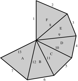
Figure 1: Wheel complex with $n=6$

We begin with the construction of $K_{1}$. We start with a structure that we call an (open) wheel: it consists of $n$ triangles incident to a wheel center vertex such that subsequent triangles share an edge, but the first and last triangles do not share an edge. The situation for $n=6$ is depicted in Figure 1. We sort the edges as depicted by numbers and the triangles in counter-clockwise orientation, as depicted by the letters. The edges with index $2$ to $7$ (and more generally, from $2$ to $n+1$) are called tire edges. Note that by design, these edges are merging components in the filtration and are, therefore negative. We call the edges remaining edges spoke edges, the edge with index $1$ the initial spoke edge, the edges with index $8$ to $12$ inner spokes edges and the last edge final spoke edge.

Next, we attach a fan of size $n$ to the final spoke edge. This means we introduce $n$ additional vertices $v_{1},\ldots,v_{n}$ and form $n$ fan triangles, each joining one $v_{i}$ with the final spoke edge. The two edges of a fan triangle, not being the final spoke edge, are called fan edges. We call the fan edge incident to the center center fan edge, and the other one outer fan edge. We sort the edges of the filtration by letting the center fan edges come after the tire edges, followed by the outer fan edges, followed by the final spoke edge.

$\left(\begin{array}[]{cccc|cccc}\ast&\ast&\ast&\ast&\ast&\ast&\ast&\ast\\ \vdots&\vdots&\vdots&\vdots&\vdots&\vdots&\vdots&\vdots\\ \ast&\ast&\ast&\ast&\ast&\ast&\ast&\ast\\ 0&0&0&1&0&0&0&0\\ 0&0&1&1&0&0&0&0\\ 0&1&1&0&0&0&0&0\\ 1&1&0&0&0&0&0&0\\ 1&0&0&0&1&1&1&1\\ \end{array}\right)$

Figure 2: (Sub)matrix of $K_{1}$

This construction yields a filtered simplicial complex whose boundary matrix contains the matrix of Figure 2 as submatrix. Note that Figure 2 is also a submatrix of the construction in [22]. The first half of the matrix contains a “staircase” of columns with decrementing pivots. The staircase is of size $4$ in the figure but can easily be extended to an arbitrary $n$ in the obvious way. The second half consists of columns that all have the same pivot, equal to the lowest step of the staircase. When reducing the matrix (using the standard or twist algorithm), the reduction of each column in the second half causes the algorithm to add each column of the first half to it in order. In total, this causes a quadratic number of column operations. The swap algorithm has the same complexity since here no swapping happens.

The retrospective algorithm, however, sparsifies the first column before it gets added to the second half. This simplification requires linear time (by one iteration through the staircase) and results in a unit vector. In all additions to the second half, the cost is therefore constant. This leads to linear complexity. It is important to note that the third nonzero entry for the left-hand-side columns comes from a tire edge, which is negative. Hence, these indices will be removed when reducing wheel triangles. Therefore, ignoring these indices, we observe that indeed the first column turns into a unit vector. Reducing the fan triangles with the retrospective algorithm thus results in removing the final spoke edge, which makes the outer fan edge the pivot, and the reduction of the column stops after one bitflip.

It remains to argue that the reduction of the edges in the filtration is linear as well for the retrospective reduction. However, this is simple to see, putting an appropriate order of the vertices in the complex. We omit the details.

For $K_{2}$, we extend the complex $K_{1}$ by adding one more vertex, called the apex, and connecting it with every vertex of the wheel via an edge. We call these edges apex edges. We sort the edges of $K_{2}$ in the following order: apex edges, center fan edges, initial spoke edge, tire edges, inner spoke edges, outer fan edges, and final spoke edge. The triangles remain in the same order as in $K_{1}$.

The two major differences to the situation of $K_{1}$ are: the tire edges are now positive edges, so the compression will not remove these entries anymore. Moreover, shifting the outer fan edges later in the filtration creates a block of $n$ edges between the inner spoke edges and the final spoke edge. The filtration boundary matrix therefore looks as depicted in Figure 3, where the just mentioned block is given between the two horizontal lines.

We see now that twist and swap reduction only cause one column addition for every column on the right because the entries in the newly inserted block prevent the algorithm from doing further reductions. Importantly, each column operation only causes a constant number of bitflips, so that the complexity is linear in the end. Again, it can easily be argued that the reduction of the edges for the twist and swap algorithm requires only linear time.

For the retrospective reduction, the addition of the first column to the second half causes a “sparsification”, as in the previous example. However, in this case, this sparsification actually turns the first column into a column with $n$ nonzero entries because it collects all indices of tire edges while iterating through the staircase. Since we then add this column $n$ times (once to every column on the right) and each addition causes $n$ bitflips, we get quadratic complexity.

$\left(\begin{array}[]{cccc|cccc}0&0&0&1&0&0&0&1\\ 0&0&1&0&0&0&1&0\\ 0&1&0&0&0&1&0&0\\ 1&0&0&0&1&0&0&0\\ 0&0&0&1&0&0&0&0\\ 0&0&1&1&0&0&0&0\\ 0&1&1&0&0&0&0&0\\ 1&1&0&0&0&0&0&0\\ \hline\cr 0&0&0&0&1&0&0&0\\ 0&0&0&0&0&1&0&0\\ 0&0&0&0&0&0&1&0\\ 0&0&0&0&0&0&0&1\\ \hline\cr 1&0&0&0&1&1&1&1\\ \end{array}\right)$

Figure 3: Matrix for $K_{2}$ (with $n=4$)

For $K_{3}$, we build up a filtration boundary matrix as depicted in Figure 4. For reference, we call the horizontal blocks in figure block 1 to block 5, starting from the bottom.

The twist algorithm applied to this boundary matrix reduces the fifth column by adding all columns on the left to it. This results in a fill-up of row indices in block 4, and the pivot being the unique row index of block 2. Since all columns on the right have the same pivot, the reduced fifth column with $n$ entries is added to every column to the right, resulting in quadratic complexity.

In the swap reduction, the fifth column is reduced in the same way. However, when added to the first column to the right, a swap happens so that in the reduction of the subsequent columns, the sixth column is used. We can observe by the block structure in block 3 that all further columns are reduced after one column addition. Also, column six has only $3$ nonzero entries, so the total complexity is linear.

To realize the depicted matrix as the boundary matrix of a simplicial complex, we again construct a wheel as in $K_{1}$. We attach one triangle to the final spoke edge, joining it with a new vertex (represented by the middle column of the matrix). Then, on the edge of that triangle not incident to the wheel center, we attach a fan of $n$ triangles. It is easily possible to sort the edges of this complex in a way that we get the depicted block structure.

Block 5
Block 4
Block 3
Block 2
Block 1

$\left(\begin{array}[]{cccc|c|cccc}\ast&\ast&\ast&\ast&\ast&\ast&\ast&\ast&\ast\\ \vdots&\vdots&\vdots&\vdots&\vdots&\vdots&\vdots&\vdots&\vdots\\ \ast&\ast&\ast&\ast&\ast&\ast&\ast&\ast&\ast\\ \hline\cr 0&0&0&1&0&0&0&0&0\\ 0&0&1&0&0&0&0&0&0\\ 0&1&0&0&0&0&0&0&0\\ 1&0&0&0&0&0&0&0&0\\ \hline\cr 0&0&0&0&0&1&0&0&0\\ 0&0&0&0&0&0&1&0&0\\ 0&0&0&0&0&0&0&1&0\\ 0&0&0&0&0&0&0&0&1\\ \hline\cr 0&0&0&0&1&1&1&1&1\\ \hline\cr 0&0&1&1&0&0&0&0&0\\ 0&1&1&0&0&0&0&0&0\\ 1&1&0&0&0&0&0&0&0\\ 1&0&0&0&1&0&0&0&0\\ \end{array}\right)$

Figure 4: Matrix for $K_{3}$ (with $n=4$)

For $K_{4}$, we build a boundary matrix as in Figure 5. For general $n$, the matrix has $n$ columns in the left block, $n$ columns in the right blocks, and exactly $3$ columns in the middle block.

For the twist reduction, the 2-nd middle column gets reduced with one column addition, resulting in a column with $4$ nonzero entries. The 3-rd middle column then has the same pivot as the just-reduced column in the middle, and the reduction of the 3-rd column requires the addition of all columns in the left block. Still, this process only requires a linear amount of bitflips. All columns on the right-hand side get added from the 2-nd column in the middle block, and because of their entries in the 3-rd row block, the reduction stops after one addition. In total, the twist reduction needs only linear time.

In the swap reduction, the difference is that at the beginning of the reduction of the 3-rd middle column, a swap happens (as the 3rd column has only $3$ nonzero entries, the 2-nd column has $4$ entries). That means that the 3-rd column in the middle gets added to all columns in the right block. Consequently, for the reduction of every column on the right, the reduction adds all the blocks on the left to it, resulting in a quadratic number of column additions.

The construction of a complex $K_{4}$ that realizes this boundary matrix can be done as follows: Similarly to $K_{3}$, we start with a wheel, attach one new triangle (that is the 3-rd column in the center), and put a fan of $n$ triangles at its outer edge (these are the columns on the right). Additionally, we attach another fan triangle (that is the 1-st center column), to the edge not containing the center, we attach another triangle (that is the 2-nd center column). The edge that is shared among the last described triangles is the last row in the matrix. The edges can easily be sorted to yield the matrix of Figure 5.

$\left(\begin{array}[]{cccc|ccc|cccc}\ast&\ast&\ast&\ast&\ast&\ast&\ast&\ast&\ast&\ast&\ast\\ \vdots&\vdots&\vdots&\vdots&\vdots&\vdots&\vdots&\vdots&\vdots&\vdots&\vdots\\ \ast&\ast&\ast&\ast&\ast&\ast&\ast&\ast&\ast&\ast&\ast\\ \hline\cr 0&0&0&0&0&0&1&0&0&0&0\\ 0&0&0&0&0&1&0&0&0&0&0\\ 0&0&0&0&0&1&0&0&0&0&0\\ 0&0&0&0&1&0&0&0&0&0&0\\ \hline\cr 0&0&0&0&0&0&0&1&0&0&0\\ 0&0&0&0&0&0&0&0&1&0&0\\ 0&0&0&0&0&0&0&0&0&1&0\\ 0&0&0&0&0&0&0&0&0&0&1\\ \hline\cr 0&0&1&1&0&0&0&0&0&0&0\\ 0&1&1&0&0&0&0&0&0&0&0\\ 1&1&0&0&0&0&0&0&0&0&0\\ 1&0&0&0&0&0&1&0&0&0&0\\ \hline\cr 0&0&0&0&1&0&1&1&1&1&1\\ 0&0&0&0&1&1&0&0&0&0&0\\ \end{array}\right)$

Figure 5: Matrix for $K_{4}$ (with $n=4$)

7 Conclusion and Discussion.

In this work, we analyzed how the sparsity of the reduced matrix correlates with the efficiency of the reduction by comparing different algorithms that keep the matrix sparse(r). The experiments show that there is no direct relation, as algorithms resulting in less sparse matrices were faster than others that aggressively sparsify. Nevertheless, the idea of keeping the matrix sparse has led us to novel reduction strategies that improve upon state-of-the-art reductions. Hence, sparsity is an important factor in fast matrix reduction.

The retrospective algorithm often achieves comparable or even better performance than the twist reduction without clearing columns. Specifically, it is consistently the fastest method for alpha shape filtrations, and it outperforms all other tested methods for shuffled filtration. Up to our knowledge, this is the first time that a method without clearing has been proven competitive in practice, which is remarkable as the clearing is the standard optimization that consistently leads to improved performances. In our experiments over a wide range of datasets, the retrospective method has regularly low fill-up compared to the other methods. We believe that the superior performance of the retrospective method is rooted in its sparsity-preserving property.

As indicated in Section 6, there is no strategy that is strictly better than others, so the best choice of reduction for a specific type of input has to be determined by comparison. We will integrate our novel variants into the PHAT library in the next release of PHAT to facilitate this comparison.

References

- [1] Ulrich Bauer. Ripser: efficient computation of Vietoris–Rips persistence barcodes. Journal of Applied and Computational Topology, pages 1–33, 2021.
- [2] Ulrich Bauer, Michael Kerber, and Jan Reininghaus. Clear and compress: Computing persistent homology in chunks. In Topological Methods in Data Analysis and Visualization III, Theory, Algorithms, and Applications, pages 103–117. Springer, 2014.
- [3] Ulrich Bauer, Michael Kerber, and Jan Reininghaus. Distributed computation of persistent homology. In 2014 proceedings of the sixteenth workshop on algorithm engineering and experiments (ALENEX), pages 31–38. SIAM, 2014.
- [4] Ulrich Bauer, Michael Kerber, Jan Reininghaus, and Hubert Wagner. Phat–persistent homology algorithms toolbox. Journal of symbolic computation, 78:76–90, 2017.
- [5] Chao Chen and Michael Kerber. Persistent homology computation with a twist. In Proceedings 27th European Workshop on Computational Geometry, 2011.
- [6] Open Scientific Visualization Datasets. https://klacansky.com/open-scivis-datasets/.
- [7] Vin de Silva, Dmitriy Morozov, and Mikael Vejdemo-Johansson. Dualities in persistent (co)homology. Inverse Problems, 27(12):124003, nov 2011.
- [8] Herbert Edelsbrunner and John Harer. Computational topology: an introduction. American Mathematical Soc., 2010.
- [9] Herbert Edelsbrunner, David Letscher, and Afra Zomorodian. Topological persistence and simplification. In Proceedings 41st annual symposium on foundations of computer science, pages 454–463. IEEE, 2000.
- [10] Herbert Edelsbrunner and Dmitriy Morozov. Persistent homology. In Handbook of Discrete and Computational Geometry, pages 637–661. Chapman and Hall/CRC, 2017.
- [11] Herbert Edelsbrunner and Katharina Ölsböck. Tri-partitions and bases of an ordered complex. Discrete & Computational Geometry, 64(3):759–775, 2020.
- [12] Herbert Edelsbrunner and Afra Zomorodian. Computing linking numbers of a filtration. Homology, Homotopy and Applications, 5(2):19–37, 2003.
- [13] Barbara Giunti, Guillaume Houry, and Michael Kerber. Average complexity of matrix reduction for clique filtrations. In Proceedings of the 2022 on International Symposium on Symbolic and Algebraic Computation, ISSAC ’22, pages 1–8, New York, NY, USA, 2022. Association for Computing Machinery.
- [14] Pierre Guillou, Jules Vidal, and Julien Tierny. Discrete morse sandwich: Fast computation of persistence diagrams for scalar data - an algorithm and A benchmark. arXiv/2206.13932, 2022.
- [15] Gregory Henselman and Robert Ghrist. Matroid filtrations and computational persistent homology. arXiv preprint 1606.00199, 2016.
- [16] Clément Jamin, Sylvain Pion, and Monique Teillaud. 3D triangulations. In CGAL User and Reference Manual. CGAL Editorial Board, 5.5 edition, 2022.
- [17] Shizuo Kaji, Takeki Sudo, and Kazushi Ahara. Cubical ripser: Software for computing persistent homology of image and volume data. arXiv preprint arXiv:2005.12692, 2020.
- [18] Richard M. Karp. Reducibility among combinatorial problems. Complexity of Computer Computations, pages 85–103, 1972.
- [19] Michael Kerber and Hannah Schreiber. Barcodes of towers and a streaming algorithm for persistent homology. Discrete & Computational Geometry, 61(4):852–879, 2019.
- [20] Ryan Lewis and Dmitriy Morozov. Parallel computation of persistent homology using the blowup complex. In Proceedings of the 27th ACM Symposium on Parallelism in Algorithms and Architectures, pages 323–331, 2015.
- [21] Nikola Milosavljević, Dmitriy Morozov, and Primož Škraba. Zigzag persistent homology in matrix multiplication time. In Proceedings of the Twenty-Seventh Annual Symposium on Computational Geometry, SoCG ’11, page 216–225, New York, NY, USA, 2011. Association for Computing Machinery.
- [22] Dmitriy Morozov. Persistence algorithm takes cubic time in worst case. BioGeometry News, Dept. Comput. Sci., Duke Univ, 2, 2005.
- [23] Nina Otter, Mason A Porter, Ulrike Tillmann, Peter Grindrod, and Heather A Harrington. A roadmap for the computation of persistent homology. EPJ Data Science, 6:1–38, 2017.
- [24] Dominik Schmid. A modification of the persistence reduction algorithm (unpublished). Master’s thesis, Graz University of Technology, 2020.
- [25] Hannah Schreiber. Algorithmic Aspects in standard and non-standard Persistent Homology. PhD thesis, Graz University of Technology, 2019.
- [26] Hubert Wagner, Chao Chen, and Erald Vuçini. Efficient computation of persistent homology for cubical data. In Topological methods in data analysis and visualization II, pages 91–106. Springer, 2012.
- [27] Simon Zhang, Mengbai Xiao, and Hao Wang. GPU-accelerated computation of Vietoris–Rips persistence barcodes. arXiv preprint arXiv:2003.07989, 2020.
- [28] A. Zomorodian and G. Carlsson. Computing persistent homology. Discrete & Computational Geometry, 33:249–274, 2005.