Geometric cumulants associated with adiabatic cycles crossing degeneracy points: Application to finite size scaling of metal-insulator transitions in crystalline electronic systems

Abstract

In this work we focus on two questions. One, we complement the machinary to calculate geometric phases along adiabatic cycles as follows. The geometric phase is a line integral along an adiabatic cycle, and if the cycle encircles a degeneracy point, the phase becomes non-trivial. If the cycle crosses the degeneracy point the phase diverges. We construct quantities which are well-defined when the path crosses the degeneracy point. We do this by constructing a generalized Bargmann invariant, and noting that it can be interpreted as a cumulant generating function, with the geometric phase being the first cumulant. We show that particular ratios of cumulants remain finite for cycles crossing a set of isolated degeneracy points. The cumulant ratios take the form of the Binder cumulants known from the theory of finite size scaling in statistical mechanics (we name them geometric Binder cumulants). Two, we show that the machinery developed can be applied to perform finite size scaling in the context of the modern theory of polarization. The geometric Binder cumulants are size independent at gap closure points or regions with closed gap (Luttinger liquid). We demonstrate this by model calculations for a one-dimensional topological model, several two-dimensional models, and a one-dimensional correlated model. In the case of two dimensions we analyze to different situations, one in which the Fermi surface is one-dimensional (a line), and two cases in which it is zero dimensional (Dirac points). For the geometric Binder cumulants the gap closure points can be found by one dimensional scaling even in two dimensions. As a technical point we stress that only certain finite difference approximations for the cumulants are applicable, since not all approximation schemes are capable of extracting the size scaling information in the case of a closed gap system.

I Introduction

Berry’s geometric phase Berry84 is an integral of a connection along a quantum adiabatic cycle. Nontrivial values arise when the curve corresponding to the adiabatic cycle encircles a degeneracy point. The geometric phase can be viewed Souza00 as the first member of a series of cumulants extracted from the evolution of the wave function along the adiabatic cycle. The higher order cumulants are not geometric, they depend on the parametrization of the cycle, not only on its geometry, but they are also physically well-defined. We show that particular ratios of the cumulants give finite values for cycles crossing degeneracy points. When the path crosses a degeneracy point, the Berry phase becomes undefined, the higher order cumulants all diverge. The machinery can not be applied in this case. In this work we complement the formalism of the geometric phase by constructing quantities which are meaningful in the case of paths which cross degeneracy (or gap closure) points.

Loosely speaking, the physical situation can be compared to electrodynamics in materials Imada98 . An insulator is a gapped system, and can be described by quantities such as the polarization, linear and nonlinear dielectric susceptibilities. In a gapless system, the polarization is undefined and the dielectric susceptibility diverges with system size. The relevant quantities become the current, the Drude weight, or the conductivity. As we will show, a similar dichotomy exists for adiabatic paths: a gapped path can be described by the Berry phase, and the gauge invariant cumulants. When gap closure occurs along the path, the relevant quantities become a particular set of cumulant ratios.

A variant of the Berry phase, known as the Zak phase Zak89 , obtained by integrating across the Brillouin zone of a crystalline system, plays the central role in the modern theory of polarization King-Smith93 ; Resta94 ; Resta00 ; Vanderbilt18 (MTP). The Zak phase is proportional to the bulk polarization of a crystalline system. It is of interest to note that our understanding of conduction and insulation in quantum systems was initiated by the seminal work of Kohn Kohn64 , who emphasized that the classical idea of localization of single charge carriers as a criterion of insulation loses its validity. Instead, the criterion of insulation, according to Kohn, is many-body localization, the localization of the center of mass of the entire charge distribution (or at least the charge distribution of large chunks of the sample). In systems with open boundaries, Kudinov Kudinov91 showed that the variance of the polarization (which is proportional to the variance of the center of mass of the charge distribution) is an appropriate criterion to distinguish conductors from insulators. For crystalline systems, however, it was not possible to calculate the center of mass of the charge distribution, nor its variance or higher cumulants, because the relevant quantum mechanical operator, the position operator, is ill-defined under periodic boundary conditions. It was precisely this problem that was solved King-Smith93 ; Resta94 ; Resta00 ; Vanderbilt18 by MTP, by casting the polarization in crystallie systems as a Zak phase.

As an extension of the MTP, Souza, Wilkens, and Martin Souza00 introduced the so called gauge invariant cumulants, which are essential in the study of polarization Marzari97 ; Marzari12 ; Watanabe18 ; Yahyavi17 as well as charge transport, since they provide access to important related quantities, such as the variance of the polarization Resta99 , or the shift current Patankar18 (related to the third cumulant). Patankar et al. Patankar18 use the ratio of the third cumulant and the second as a gauge of nonlinearity in the Su-Schrieffer-Heeger model Su79 . The Zak phase Zak89 is also the starting point to construct topological invariants, the quantities which characterize the different phases of topological insulators Bernevig13 ; Haldane88 ; Kane13 ; Kane05a ; Kane05b . The MTP formalism has also been applied Thonhauser06 to study the topological Haldane model.

A limitation of the quantities derived from the MTP is that at gap closure information about system size scaling is lost. The variance of the polarization, as derived by Resta, diverges at gap closure, even for finite systems. For this reason, techniques based on the finite size scaling hypothesis Fisher72a ; Fisher72b are not directly applicable to metal-insulator transitions. Application of the Binder cumulant technique Binder81a ; Binder81b (based on the finite size scaling hypothesis) in MTP is difficult for two reasons: other than the loss of size scaling information already mentioned, a Binder cumulant is a ratio of averages of expectation values of observables (the order parameter), and in MTP the basic quantity is a geometric phase, rather than the expectation value of an observable. In this work we overcome both of these obstacles.

Cumulants are logarithmic derivatives of characteristic functions (also known as cumulant generating functions). Since there exist cumulants in the context of the Zak phase, we first show that for general geometric phases (not necessarily a Zak phase) a generalization of the Bargmann invariant Bargmann64 plays the role of the characteristic function. The generalized Bargmann invariant is most closely related to the characteristic function of a periodic probability distribution, since moments and cumulants can be obtained from it via finite difference derivatives.

Our construction of cumulant ratios is similar to that of the Binder cumulants Binder81a ; Binder81b , for this reason, we will use the term geometric Binder cumulant (GBC). The GBCs are zero if the adiabatic path encounters no gap closure points, otherwise they are finite. As a preliminary example, we calculate the GBC for a spin-$\frac{1}{2}$ particle in a precessing magnetic field. We then implement our construction in the MTP King-Smith93 ; Resta94 ; Resta00 ; Vanderbilt18 ; Thonhauser06 and show that the GBCs are an effective tool for finite size scaling of metal-insulator Imada98 and other quantum phase transitions. Gap closure points (or regions) can be located. As a technicality, we emphasize the use of a particular application of finite difference derivatives which guarantee the correct scaling with system size in gapless systems.

We also investigate the applicability of the MTP to two-dimensional and one-dimensional interacting systems. In the former, the set of gap closure points can be one or zero dimensional (Dirac points in graphene). The question we pose is whether the cumulants constructed within the MTP can signal a zero dimensional gap closure. We find in cases such as graphene (or the Haldane model) scaling has to be done in one dimension only. As for the interacting system we study, the Berry phase corresponding to the polarization is a single-point Berry phase. Nevertheless, the gap closure region is located via application of the GBC.

In section II, for background, we introduce the characteristic function and show how moments and cumulants are generated from it. We emphasize the distinction between a general and a periodic probability distribution function. In the former, moments and cumulants are obtained via derivatives, while in the latter one has to resort to finite difference derivatives. In section III we use the Bargmann invariant Bargmann64 as a starting point to derive the GBCs. In section IV basic calculations are presented for a spin-$\frac{1}{2}$ particle in a rotating magnetic field. In section V we construct GBCs for the finite scaling of the polarization, emphasizing the importance of an alternative approximation scheme which gives the correct size scaling information at gap closure. In section VI we give expressions for the variance of the polarization and the GBC at different approximation levels for an ideal conductor (gap closure point). In section VII we present model calculations for one and two-dimensional band insulators, as well as for a correlated system. In section VIII we conclude our work.

II Background: moments, central moments, cumulants and Binder cumulants

To initiate the discussion we give an overview of some quantities used in statistics to characterize probability distributions. Given a real random variable $x$ and a probability distribution $P(x)$ which satisfies

$$P(x)\geq 0;\int_{-\infty}^{\infty}dxP(x)=1.$$ (1)

The characteristic function $f(k)$ is the Fourier transform of $P(x)$,

$$f(k)=\int_{-\infty}^{\infty}dxP(x)e^{ikx}.$$ (2)

The $n$th moment of the distribution $P(x)$ is defined as

$$M_{n}=\frac{1}{i^{n}}\left.\frac{\partial^{n}f(k)}{\partial k^{n}}\right|_{k=0}=\langle x^{n}\rangle.$$ (3)

The $n$th cumulant of $P(x)$ is defined as

$$C_{n}=\frac{1}{i^{n}}\left.\frac{\partial^{n}\ln f(k)}{\partial k^{n}}\right|_{k=0}.$$ (4)

Cumulants can be written in terms of moments (and vice versa). For the first four cumulants the expressions in terms of moments are:

$$C_{1} = M_{1},$$ (5)

$$C_{2} = M_{2}-M_{1}^{2},$$

$$C_{3} = M_{3}-3M_{2}M_{1}+2M_{1}^{3},$$

$$C_{4} = M_{4}-4M_{3}M_{1}-3M_{2}^{2}+12M_{2}M_{1}^{2}-6M_{1}^{4}.$$

The first four cumulants are named as follows: $C_{1}$ the mean, $C_{2}$ the variance, $C_{3}$ the skew, and $C_{4}$ is the kurtosis. Cumulants of order higher than one are independent of the mean or the origin of the coordinate system.

It is possible to define the central moments, which are the moments derived from the probability distribution $P(x)\rightarrow P(x+M_{1})$, shifted to give a zero first moment. $M_{1}$ is the first moment of the unshifted distribution. Using the shifted probability distribution in Eq. (4) to derive cumulants results in

$$C_{1} = 0,$$ (6)

$$C_{2} = M_{2},$$

$$C_{3} = M_{3},$$

$$C_{4} = M_{4}-3M_{2}^{2}.$$

Note that if $P(x)$ is shifted, it is the phase of the corresponding characteristic function that shifts,

$$f(k)\rightarrow f(k)e^{-ikM_{1}}.$$ (7)

We now consider a distribution periodic in $L$,

$$P_{L}(x)=\sum_{w=-\infty}^{\infty}P(x+wL).$$ (8)

In this case, the characteristic function associated with $P_{L}(x)$ is discrete,

$$f_{q}=\int_{0}^{L}dxP_{L}(x)e^{i2\pi qx/L};q\in\mathbb{Z}.$$ (9)

Substituting Eq. (8) into Eq. (9) we see that

$$f_{q}=f\left(\frac{2\pi}{L}q\right),$$ (10)

where the right hand side is the characteristic function of the distribution $P(x)$ (Eq. (2)) evaluated at $k=\frac{2\pi}{L}q$.

Since for periodic distributions the characteristic function is only well-defined at a discrete set of $k$-points, the moments and cumulants have to be based on finite difference derivatives of $f_{q}$, rather than continuous derivatives. We define them as follows:

$$M_{n}=\begin{cases}(-1)^{\frac{n-1}{2}}\left(\frac{L}{2\pi}\right)^{n}\mbox{Im}\left.\frac{\mathbb{D}^{n}f_{q}}{\mathbb{D}q^{n}}\right|_{q=0}&\mbox{if $n$ is odd},\\ \hskip 8.5359pt(-1)^{\frac{n}{2}}\left(\frac{L}{2\pi}\right)^{n}\mbox{Re}\left.\frac{\mathbb{D}^{n}f_{q}}{\mathbb{D}q^{n}}\right|_{q=0}&\mbox{if $n$ is even}.\end{cases}$$ (11)

$$C_{n}=\begin{cases}(-1)^{\frac{n-1}{2}}\left(\frac{L}{2\pi}\right)^{n}\mbox{Im}\left.\frac{\mathbb{D}^{n}\ln f_{q}}{\mathbb{D}q^{n}}\right|_{q=0}&\mbox{if $n$ is odd},\\ \hskip 8.5359pt(-1)^{\frac{n}{2}}\left(\frac{L}{2\pi}\right)^{n}\mbox{Re}\left.\frac{\mathbb{D}^{n}\ln f_{q}}{\mathbb{D}q^{n}}\right|_{q=0}&\mbox{if $n$ is even}.\end{cases}$$ (12)

where the notation $\frac{\mathbb{D}}{\mathbb{D}q}$ denotes a finite difference derivative. There are different types of finite difference approximations Hildebrand68 . We will adhere to the convention introduced by Resta and Sorella in the context of the modern theory of polarization, and use central difference approximations in all cases. Unless otherwise indicated, we use the lowest order approximation, but in sections VI and VII we will make comparisons between approximations of different orders.

Applying the lowest order finite difference approximation results in

$$C_{1} = \frac{L}{2\pi}\mbox{Im}\frac{\ln f_{1}-\ln f_{-1}}{2}=\frac{L}{2\pi}\mbox{Im}\ln f_{1},$$ (13)

$$C_{2} = -\left(\frac{L}{2\pi}\right)^{2}\mbox{Re}(\ln f_{1}+\ln f_{-1}-2\ln f_{0})$$

$$= -\frac{L^{2}}{2\pi^{2}}\mbox{Re}\ln f_{1},$$

where we used that $f_{q}=f_{-q}^{*}$ and that $f_{0}=1$. Note the similarity of the $C_{1}$ and $C_{2}$ in Eq. (13) to the Resta Resta98 and Resta-Sorella Resta99 expressions for the polarization and its variance. In the limit $L\rightarrow\infty$ $C_{1}$ and $C_{2}$ converge to $\langle x\rangle$ and $\langle x^{2}\rangle-\langle x\rangle^{2}$, respectively, and higher order cumulants constructed via Eq. (4) also reproduce the cumulants (Eq. (4)).

The Binder cumulant Binder81a ; Binder81b is a quantity used to locate phase transition points and critical exponents. It is an application of the finite size scaling hypothesis Fisher72a ; Fisher72b . In numerical simulations the thermodynamic limit is not accessible, for this reason, phase transition points can be shifted or smeared out when numerically calculated based on susceptibilities or other response functions. These numerical artifacts are eliminated at phase transition points by the use of the Binder cumulant. The method is useful in classical Selke06 as well as quantum Hetenyi99 phase transitions, however, heretofore the construction has only been applied in phase transitions characterized by order parameters, i.e. expectation values of Hermitian operators.

In the construction due to Binder, particular ratios of moments (or cumulants) are taken. The Binder cumulants take known values at phase transition points which are independent of system size. It is this property which makes the Binder cumulant a computationally useful tool in locating critical points. One commonly used Binder cumulant is

$$U_{4}=1-\frac{1}{3}\frac{M_{4}}{M_{2}^{2}}=-\frac{1}{3}\frac{C_{4}}{C_{2}^{2}}.$$ (14)

The crucial point is that the product of the orders of moments in the numerator and the denominator are equal. This is the reason the size dependence cancels at critical points.

III Moments, central moments, cumulants, and Binder cumulants associated with adiabatic cycles

In this section we derive the Berry phase. We show that the Berry phase can be viewed as the first in a cumulant sequence associated with the Bargmann invariant. An extended version of the Bargmann invariant will take the place of the characteristic function, and from it the above mentioned cumulant sequence can be derived through the application of finite difference derivatives, as was done in Eqs. (11) and (12). We also show that ratios of moments constructed á la Binder are physically well defined geometric quantities (the GBC). In subsequent sections we show that they take non-trivial values when the adiabatic path encounters a degeneracy point.

By adiabatic cycle we mean a cycle for which the adiabatic theorem holds. This theorem was first proven by Born and Fock Born28 for the nondegenerate case. They considered paths along which the particular state under consideration is gapped, as well as paths along which level crossings occur at a finite number of singular points along the path. Kato Kato50 generalized the results of Born and Fock to the case of degenerate states. The paths considered in this case are such that a set of degenerate states are isolated from the rest of the Hilbert space of the system via an energy gap, but, again, a finite number of gap closures with other sets of degenerate states can occur at crossing points.

To derive the Berry phase and cumulants valid for the general case, we consider a parameter space $\vec{\bf\xi}$. At each point of this parameter space a Hamiltonian is defined, for which it is valid that

$$H(\vec{\bf\xi})|\Psi_{n}(\vec{\bf\xi})\rangle=E_{n}(\vec{\bf\xi})|\Psi_{n}(\vec{\bf\xi})\rangle,$$ (15)

where $E_{n}(\vec{\bf\xi})$($|\Psi_{n}(\vec{\bf\xi})\rangle$) denote energy eigenvalues(eigenstates). We will consider the ground state, $|\Psi_{0}(\vec{\bf\xi})\rangle$, but the construction is general. We consider a set of points in the parameter space, $\vec{\bf\xi}_{m}$ with $m=1,...,N$, and form the discrete Berry phase based on the cyclic product,

$$\tilde{Z}_{q}=\prod_{m=1}^{N}\langle\Psi(\vec{\bf\xi}_{m})|\Psi(\vec{\bf\xi}_{m+q})\rangle,$$ (16)

where $\vec{\bf\xi}_{N+s}$ is set equal to $\vec{\bf\xi}_{s}$, and where the index for the ground state, subscript $0$, was suppressed. The cyclic product $\tilde{Z}_{1}$ is known as the Bargmann invariant Bargmann64 . $\tilde{Z}_{q}$ is the general discrete cumulant generating function, an extension of the Bargmann invariant. The series of moments or cumulants can be generated from $\tilde{Z}_{q}$ by setting $f_{q}=\tilde{Z}_{q}$, and using Eqs. (11) and (12) and by applying finite difference derivative formulas with respect to the discrete variable $q$. The interval in this case is not $frac{L}{2\pi}$, but unity.

The first cumulant that results from this procedure is the discrete Berry phase,

$$C_{1}=\mbox{Im}\left.\frac{\mathbb{D}\ln Z_{q}}{\mathbb{D}q}\right|_{q=0}=\mbox{Im}(\ln\tilde{Z}_{1}-\ln\tilde{Z}_{0})=\mbox{Im}\ln\tilde{Z}_{1},$$ (17)

since $\tilde{Z}_{0}=1$. Some of the higher order cumulants may be written,

$$C_{2} = -2\mbox{Re}\ln\tilde{Z}_{1}$$ (18)

$$C_{3} = -\mbox{Im}\ln\tilde{Z}_{2}+2\mbox{Im}\ln\tilde{Z}_{1},$$

$$C_{4} = 2\mbox{Re}\ln\tilde{Z}_{2}-8\mbox{Re}\ln\tilde{Z}_{1}.$$

Odd cumulants are sums of phases of $\tilde{Z}_{q}$, even ones are sums of the logarithms of their magnitudes. The continuous Berry phase can be derived from Eqs. (16) and (17) by assuming that the parameter series $\vec{\bf\xi}_{m}$ is placed along a closed curve in the order $m=1,...,N$. We can take the continuous limit by increasing $N$, the number of points representing the closed curve (simultaneously decrease the distances between them). We can then use the expansion up to first order

$$|\Psi(\vec{\bf\xi}_{m+1})\rangle=|\Psi(\vec{\bf\xi}_{m})\rangle+\delta{\vec{\xi}}\cdot\nabla_{\vec{\bf\xi}}|\Psi(\vec{\bf\xi}_{m})\rangle,$$ (19)

to rewrite $C_{1}$ as

$$C_{1}=\mbox{Im}\sum_{m=1}^{N}\delta{\vec{\xi}}\cdot\langle\Psi(\vec{\bf\xi}_{m})|\nabla_{\vec{\bf\xi}}|\Psi(\vec{\bf\xi}_{m})\rangle,$$ (20)

or, in the continuous limit,

$$C_{1}=\mbox{Im}\oint d\vec{\bf\xi}\cdot\langle\Psi(\vec{\bf\xi})|\nabla_{\vec{\bf\xi}}|\Psi(\vec{\bf\xi})\rangle.$$ (21)

It is useful to introduce a parametrization for the closed curve in parameter space as $\vec{\xi}(t)$, where $t\in[0,T]$. We now discretize as $t_{m}=m\delta t$ (with $\delta t=\frac{T}{N}$). In this case, the discrete path Berry phase (20) can be written as

$$C_{1}=\mbox{Im}\sum_{m=1}^{N}\delta t\langle\Psi(t_{m})|\partial_{t}|\Psi(t_{m})\rangle,$$ (22)

or in the continuous limit,

$$C_{1}=\mbox{Im}\int_{0}^{T}dt\langle\Psi(t)|\partial_{t}|\Psi(t)\rangle.$$ (23)

Expanding $\ln\tilde{Z}_{1}$ to second order, and using the definition of $C_{2}$ (Eq. (18)) results in,

$$C_{2} = -\sum_{m=1}^{N}\left[\langle\Psi(\vec{\bf\xi}_{m})|(\delta{\vec{\xi}}\cdot\nabla_{\vec{\bf\xi}})^{2}|\Psi(\vec{\bf\xi}_{m})\rangle\right.$$

$$-\left.\langle\Psi(\vec{\bf\xi}_{m})|(\delta{\vec{\xi}}\cdot\nabla_{\vec{\bf\xi}})|\Psi(\vec{\bf\xi}_{m})\rangle^{2}\right],$$

or using the parametrization

$$C_{2} = -\delta t^{2}\sum_{m=1}^{N}\left[\langle\Psi(t_{m})|\partial_{t}^{2}|\Psi(t_{m})\rangle\right.$$

$$-\left.\langle\Psi(t_{m})|\partial_{t}|\Psi(t_{m})\rangle^{2}\right].$$

The continuous limit can only be taken in Eq. (III), not in Eq. (III). In Eq. (III) one factor of $\delta t$ has to be eliminated, and only then do we obtain

$$\Gamma_{2} = -\int_{0}^{T}dt\left[\langle\Psi(t)|\partial_{t}^{2}|\Psi(t)\rangle\right.$$

$$-\left.\langle\Psi(t)|\partial_{t}|\Psi(t)\rangle^{2}\right].$$

$\Gamma_{2}$ is physically well-defined, however, it is no longer geometric. It is not merely a function of the cyclic path, it also depends on “how fast” the path is traversed in the variable $t$. $\Gamma_{2}$ gives finite numbers for adiabatic paths which do not encounter crossing points. The situation is similar for all higher order cumulants. An $n$th order $C_{n}$ will lead to a factor of $\delta t^{n}$, from which $n-1$ have to be eliminated to lead to a $\Gamma_{n}$ which is physically well-defined, albeit, not geometric. Cumulants constructed this way are known as gauge invariant cumulants, introduced in the context of the MTP by Souza, Wilkens, and Martin Souza00 .

Characteristic	Definition	Associated	Moments, cumulants
function		with
$f(k)$	$=\int_{-\infty}^{\infty}dx\exp(ikx)P(x)$	$P(x)$, probability distribution	$M_{n}=\frac{1}{i^{n}}\left.\frac{\partial^{n}f(k)}{\partial k^{n}}\right|_{k=0}$
		of a continuous random variable	$C_{n}=\frac{1}{i^{n}}\left.\frac{\partial^{n}\ln f(k)}{\partial k^{n}}\right|_{k=0}$
$f_{q}$	$=\int_{0}^{L}dx\exp\left(i\frac{2\pi x}{L}q\right)P_{L}(x)$	$P_{L}(x)$, probability distribution	$M_{n}=\begin{cases}(-1)^{\frac{n-1}{2}}\left(\frac{L}{2\pi}\right)^{n}\mbox{Im}\left.\frac{\mathbb{D}^{n}f_{q}}{\mathbb{D}q^{n}}\right|_{q=0}&\mbox{if $n$ is odd},\\ \hskip 8.5359pt(-1)^{\frac{n}{2}}\left(\frac{L}{2\pi}\right)^{n}\mbox{Re}\left.\frac{\mathbb{D}^{n}f_{q}}{\mathbb{D}q^{n}}\right|_{q=0}&\mbox{if $n$ is even}.\end{cases}$
	$q$ integer	of a continuous random variable	$C_{n}=\begin{cases}(-1)^{\frac{n-1}{2}}\left(\frac{L}{2\pi}\right)^{n}\mbox{Im}\left.\frac{\mathbb{D}^{n}\ln f_{q}}{\mathbb{D}q^{n}}\right|_{q=0}&\mbox{if $n$ is odd},\\ \hskip 8.5359pt(-1)^{\frac{n}{2}}\left(\frac{L}{2\pi}\right)^{n}\mbox{Re}\left.\frac{\mathbb{D}^{n}\ln f_{q}}{\mathbb{D}q^{n}}\right|_{q=0}&\mbox{if $n$ is even}.\end{cases}$
		periodic in $L$
$\tilde{Z}_{q}$	$=\prod_{s=1}^{N}\langle\Psi(\xi_{s})|\Psi(\xi_{s+q}\rangle$	geometric phases	$M_{n}=\begin{cases}(-1)^{\frac{n-1}{2}}\mbox{Im}\left.\frac{\mathbb{D}^{n}\tilde{Z}_{q}}{\mathbb{D}q^{n}}\right|_{q=0}&\mbox{if $n$ is odd},\\ \hskip 8.5359pt(-1)^{\frac{n}{2}}\mbox{Re}\left.\frac{\mathbb{D}^{n}\tilde{Z}_{q}}{\mathbb{D}q^{n}}\right|_{q=0}&\mbox{if $n$ is even}.\end{cases}$
	$q$ integer	along adiabatic cycles	$C_{n}=\begin{cases}(-1)^{\frac{n-1}{2}}\mbox{Im}\left.\frac{\mathbb{D}^{n}\ln\tilde{Z}_{q}}{\mathbb{D}q^{n}}\right|_{q=0}&\mbox{if $n$ is odd},\\ \hskip 8.5359pt(-1)^{\frac{n}{2}}\mbox{Re}\left.\frac{\mathbb{D}^{n}\ln\tilde{Z}_{q}}{\mathbb{D}q^{n}}\right|_{q=0}&\mbox{if $n$ is even}.\end{cases}$
$Z_{q}$	$=\langle\Psi_{0}|\exp\left(i\frac{2\pi\hat{X}}{L}q\right)|\Psi_{0}\rangle$	polarization distribution	$M_{n}=\begin{cases}(-1)^{\frac{n-1}{2}}\left(\frac{L}{2\pi}\right)^{n}\mbox{Im}\left.\frac{\mathbb{D}^{n}Z_{q}}{\mathbb{D}q^{n}}\right|_{q=0}&\mbox{if $n$ is odd},\\ \hskip 8.5359pt(-1)^{\frac{n}{2}}\left(\frac{L}{2\pi}\right)^{n}\mbox{Re}\left.\frac{\mathbb{D}^{n}Z_{q}}{\mathbb{D}q^{n}}\right|_{q=0}&\mbox{if $n$ is even}.\end{cases}$
	$q$ integer	of many-body systems	$C_{n}=\begin{cases}(-1)^{\frac{n-1}{2}}\left(\frac{L}{2\pi}\right)^{n}\mbox{Im}\left.\frac{\mathbb{D}^{n}\ln Z_{q}}{\mathbb{D}q^{n}}\right|_{q=0}&\mbox{if $n$ is odd},\\ \hskip 8.5359pt(-1)^{\frac{n}{2}}\left(\frac{L}{2\pi}\right)^{n}\mbox{Re}\left.\frac{\mathbb{D}^{n}\ln Z_{q}}{\mathbb{D}q^{n}}\right|_{q=0}&\mbox{if $n$ is even}.\end{cases}$
		periodic in $L$
$Z_{q}^{(b)}$	$=\mbox{Det}\prod_{s=1}^{L}S(k_{s},k_{s+q})$	polarization distribution	$M_{n}=\begin{cases}(-1)^{\frac{n-1}{2}}\left(\frac{L}{2\pi}\right)^{n}\mbox{Im}\left.\frac{\mathbb{D}^{n}Z_{q}^{(b)}}{\mathbb{D}q^{n}}\right|_{q=0}&\mbox{if $n$ is odd},\\ \hskip 8.5359pt(-1)^{\frac{n}{2}}\left(\frac{L}{2\pi}\right)^{n}\mbox{Re}\left.\frac{\mathbb{D}^{n}Z_{q}^{(b)}}{\mathbb{D}q^{n}}\right|_{q=0}&\mbox{if $n$ is even}.\end{cases}$
	$S(k_{s},k_{s+q})=\langle u_{k_{s},m}|u_{k_{s+q},m^{\prime}}\rangle$	of band systems
	$q$ integer,	periodic in $L$	$C_{n}=\begin{cases}(-1)^{\frac{n-1}{2}}\left(\frac{L}{2\pi}\right)^{n}\mbox{Im}\left.\frac{\mathbb{D}^{n}\ln Z_{q}^{(b)}}{\mathbb{D}q^{n}}\right|_{q=0}&\mbox{if $n$ is odd},\\ \hskip 8.5359pt(-1)^{\frac{n}{2}}\left(\frac{L}{2\pi}\right)^{n}\mbox{Re}\left.\frac{\mathbb{D}^{n}\ln Z_{q}^{(b)}}{\mathbb{D}q^{n}}\right|_{q=0}&\mbox{if $n$ is even}.\end{cases}$
	$m,m^{\prime}$ occupied bands
	$|u_{k_{s},m^{\prime}}\rangle$ periodic Bloch state

Table 1: Different types of characteristic functions (cumulant generating functions) discussed in this work. The definitions of the characteristic functions are given in the second column. The third column specifies the contexts in which they appear. The fourth column specifies how moments ($M_{n}$) and cumulants ($C_{n}$) are obtained from the characteristic functions. The notation $\frac{\mathbb{D}^{n}...}{\mathbb{D}q^{n}}$ denotes an $n$th finite difference derivative.

It is possible to construct quantities which are gauge invariant as well as geometric. Let us first write $C_{4}$ as

$$C_{4} = \delta t^{4}\sum_{m=1}^{N}\left[\langle\Psi(t_{m})|\partial_{t}^{4}|\Psi(t_{m})\rangle\right.$$

$$\left.-4\langle\Psi(t_{m})|\partial_{t}^{3}|\Psi(t_{m})\rangle\langle\Psi(t_{m})|\partial_{t}|\Psi(t_{m})\rangle\right.$$

$$\left.-3\langle\Psi(t_{m})|\partial_{t}^{2}|\Psi(t_{m})\rangle\langle\Psi(t_{m})|\partial_{t}^{2}|\Psi(t_{m})\rangle\right.$$

$$\left.+12\langle\Psi(t_{m})|\partial_{t}^{2}|\Psi(t_{m})\rangle\langle\Psi(t_{m})|\partial_{t}|\Psi(t_{m})\rangle^{2}\right.$$

$$\left.-6\langle\Psi(t_{m})|\partial_{t}|\Psi(t_{m})\rangle^{4}\right].$$

The quantity

$$U_{4}=-\lim_{\delta t\rightarrow 0}\frac{1}{3}\frac{C_{4}}{C_{2}^{2}},$$ (28)

is gauge invariant and geometric, where $C_{4}$ and $C_{2}$ are defined as in Eqs. (III) and (III), respectively. In Eq. (28) the $\delta t$s cancel, because, as is the case in the original Binder cumulants, the products of the orders of the cumulants in the numerator and the denominator are equal.

If the adiabatic path does not encounter a gap closure point, then $U_{4}=0$. Defining $C_{4}=\delta t^{3}\Gamma_{4}$, and taking the limit $\delta t\rightarrow 0$ results in

$$U_{4}=\lim_{\delta t\rightarrow 0}\delta t\frac{\Gamma_{4}}{\Gamma_{2}^{2}}\rightarrow 0.$$ (29)

($\Gamma_{4}$ does take finite values for adiabatic paths which do not encounter degeneracy points.) However, $U_{4}$ gives a finite value if the adiabatic path does encounter a degeneracy point.

IV Spin-$\frac{1}{2}$ particle in a rotating magnetic field

In this section we calculate $U_{4}$ for a spin-$\frac{1}{2}$ particle in a rotating magnetic field. This system was used as an example in the original work of Berry Berry84 to demonstrate the meaning of the Berry phase arising through adiabatic paths which encircle the degeneracy. Here we show what happens when the path touches the degeneracy point.

The Hamiltonian of a spin-$\frac{1}{2}$ particle in a magnetic field is given by

$$H=-g\frac{e}{2m_{e}}\vec{\bf S}\cdot\vec{\bf B},$$ (30)

where

$$\vec{\bf S}=\frac{\hbar}{2}\vec{\bf\sigma},$$ (31)

and $\vec{\bf\sigma}$ is a vector of Pauli matrices, $\sigma_{x}$, $\sigma_{y}$, and $\sigma_{z}$. We assume that the magnetic field $\vec{\bf B}$ is time-dependent and precesses at frequency $\omega$ according to

$$B_{x} = B\sin(\theta)\cos(\omega t)$$ (32)

$$B_{y} = B\sin(\theta)\sin(\omega t)$$

$$B_{z} = B\cos(\theta).$$

We set $\phi=\omega t$. This system can be solved exactly. The solution we use to construct moments has the form

$$|\Psi_{-}(\theta,\phi)\rangle=\left({\begin{array}[]{c}-e^{i\phi}\sin\left(\frac{\theta}{2}\right)\\ \cos\left(\frac{\theta}{2}\right)\end{array}}\right).$$ (33)

Using $|\Psi_{-}(\theta,\phi)\rangle$ we construct a $Z_{q}$ along a path in the space $\vec{\bf B}$ discretized according to $\phi_{m}=m\frac{2\pi}{N}$, with $m=1,...,N$, resulting in,

$$\tilde{Z}_{q}=\left(\sin^{2}\frac{\theta}{2}e^{i\frac{2\pi}{N}q}+\cos^{2}\frac{\theta}{2}\right)^{N}.$$ (34)

From Eq. (11) it can be shown that

$$M_{4} = 2(|\tilde{Z}_{2}|-4|\tilde{Z}_{1}|+3)$$ (35)

$$M_{2} = 2(|\tilde{Z}_{1}|-1),$$

(the magnitudes of all the $\tilde{Z}_{q}$s were taken, to center the “distribution”) and using Eq. (34) it follows that

$$\frac{M_{4}}{M_{2}^{2}}=3,$$ (36)

implying that $U_{4}$, as defined in Eq. (14) is zero.

The gap closure of this system occurs at the origin. We can also consider a cyclic path which crosses this point. In this case, since for all $n\neq 0$ $Z_{n}=0$, and $Z_{0}=1$, we obtain,

$$\frac{M_{4}}{M_{2}^{2}}=\frac{3}{2},$$ (37)

implying that $U_{4}$ is $\frac{1}{2}$. The GBC gives a finite number for a cyclic path which encounters the degeneracy point.

The above result is valid for any parametrization of the adiabatic loop. The fact that the GBC is finite for a loop which encounters the degeneracy point is due to the fact that in the product on the right-hand side of Eq. (16) the scalar product “across” the degeneracy point gives zero, and therefore the entire product will be zero. Reparametrizing the loop will not change this. Also, the direction of the path as it crosses the degeneracy point is not important either, since the result that $n\neq 0$ $Z_{n}=0$, and $Z_{0}=1$ is independent of direction.

V Cumulants of the polarization

In this section, we make the connection between the cumulant machinery and the MTP explicit. We first show that the quantity which plays the central role in MTP, sometimes called Watanabe18 the polarization amplitude (defined below in Eq. (38)), is a discrete characteristic function of the type derived in Eq. (9). As such, the cumulants Resta98 ; Resta99 can only be derived via finite difference derivatives. Second, we show that if we evaluate the polarization amplitude for a band insulator (where the wave function is a Slater determinant), then it takes the form of the generalized Bargmann invariant defined in Eq. (16). This derivation links the quantities introduced in Sections II and III.

We consider a many-electron system, one-dimensional for convenience, periodic in $L$. In our calculations below, $L$ will always refer to the size of the supercell of the system, in which periodic boundary conditions are imposed. In band systems $2\pi/L$ is the spacing between k-points in the Brillouin zone. We write the quantity known as the polarization amplitude as,

$$Z_{q}=\langle\Psi_{0}|\exp\left(i\frac{2\pi q}{L}\hat{X}\right)|\Psi_{0}\rangle,$$ (38)

where $\Psi_{0}$ denotes the ground state wave function of the system, $q$ is an integer, and the total position operator is defined as

$$\hat{X}=\sum_{j=1}^{L}\hat{n}_{j}j,$$ (39)

where $\hat{n}_{j}$ is the density operator at site $j$.

To show that $Z_{q}$ is the analog of a characteristic function we can write the distribution of the total position corresponding to the state $\Psi_{0}$

$$P_{L}(X)=\langle\Psi_{0}|\delta(\hat{X}-X)|\Psi_{0}\rangle.$$ (40)

The distribution $P_{L}(X)$ is manifestly periodic in $L$. We can write $Z_{q}$ as

$$Z_{q}=\int dXP_{L}(X)\exp\left(i\frac{2\pi q}{L}X\right).$$ (41)

It is obvious that $Z_{q}$ is a discrete characteristic function of the type given in Eq. (9). We can derive the $n$th moment or cumulant of $X$ by applying Eqs. (11) and (12).

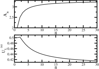
Figure 1: $A_{n}$ (defined in Eq. (59)) as a function of $n$ (upper panel). The Binder cumulant as a function of $n$ for a gapless system.

The electronic contribution to the polarization can be obtained from $Z_{q}$ by taking the first finite difference derivative with respect to $q$. Indeed, the electronic contribution to the many-body polarization expression derived by Resta Resta98 for interacting systems can be derived by taking the first finite difference derivative of $\ln Z_{q}$ at $q=0$,

$$\langle X\rangle=i\frac{L}{2\pi}\left(\ln Z_{1}-\ln Z_{0}\right)=\frac{L}{2\pi}\mbox{Im}\ln Z_{1}.$$ (42)

To obtain the full polarization, the nuclear contribution Souza00 ; Resta00 also has to be added. In most models of interest (tight-binding type models) the nuclei are taken as fixed in position. Therefore, the nuclei do make a contribution to the first cumulant (the polarization), but since higher order cumulants describe fluctuations, the nuclei make no contribution.

We now show that for a band insulator, it is possible to relate $Z_{q}$, as defined in Eq. (38) to the generalized Bargmann invariant of Eq. (16). We can follow the steps of Resta Resta98 , and introduce a system periodic in $L$, with lattice constant taken to be unity. We will consider a system with one filled band, but we will comment on the many-band generalization below. The $L$ Bloch vectors in the reciprocal cell $[0,2\pi/L)$ can be labelled,

$$k_{s}=\frac{2\pi}{L}s,s=0,...,L-1,$$ (43)

and the one-body orbitals will have the form

$$\psi_{k_{s}}(x)=e^{ik_{s}x}u_{k_{s}}(x),$$ (44)

where $u_{k_{s}}(x)$ is a periodic Bloch function. The entire wave function can be written as

$$|\Psi_{0}\rangle=\mathbb{A}\prod_{s=0}^{L-1}\psi_{k_{s}},$$ (45)

where $\mathbb{A}$ is the anti-symmetrization operator. Using this wave function to write $Z_{q}$ (Eq. (38)) results in

$$Z_{q}^{(b)}=\prod_{s=1}^{L}S(k_{s},k_{s+q}),$$ (46)

where $Z_{q}^{(b)}$ indicates the quantity in Eq. (38) averaged over a single Slater determinant representing an electronic band, and where

$$S(k_{s},k_{s+q})=\langle u_{k_{s}}|u_{k_{s+q}}\rangle,$$ (47)

hence, it takes the form of Eq. (16).

The extension to more than one filled band turns $S(k_{s},k_{s+q})$ into a matrix, and $Z_{q}$ into a determinant of the product of matrices,

$$Z_{q}^{(b)}=\mbox{Det}\prod_{s=1}^{L}S(k_{s},k_{s+q}),$$ (48)

where

$$S(k_{s},k_{s+q})=\langle u_{k_{s},m}|u_{k_{s+q},m^{\prime}}\rangle,$$ (49)

where $m$ and $m^{\prime}$ are band indices. For $q=1$, we recover the known quantity used to derive King-Smith93 ; Resta94 ; Resta00 ; Vanderbilt18 the MTP. For reference, and as a partial summary, in table I we summarize the different types of characteristic functions encountered in this work.

We now analyze the implementation of he finite difference derivatives in the MTP. We first quote the Resta-Sorella expression for the variance,

$$C_{2}^{(RS1)}=-\frac{L^{2}}{2\pi^{2}}\mbox{Re}\ln Z_{1},$$ (50)

according to the lowest order finite difference approximation (RS1). This scheme has error $\mathcal{O}\left(L^{-2}\right)$. An error of order $\mathcal{O}\left(L^{-4}\right)$ can be achieved by using a higher order finite difference derivative,

$$C_{2}^{(RS2)}=\frac{L^{2}}{24\pi^{2}}\left[\mbox{Re}\ln Z_{2}-16\mbox{Re}\ln Z_{1}\right].$$ (51)

We would like to point out that when the expression $C_{2}^{(RS1)}$ (or higher order finite difference approximations, such as $C_{2}^{(RS2)}$) is applied to analyze quantum phase transitions, which are accompanied by gap closure, a problem is encountered. In the case of an ideal conductor the twist operator shifts all the momenta of the system producing a state which is orthogonal to the ground state:

$$|\Psi_{0}\rangle\perp\exp\left(i\frac{2\pi q}{L}\hat{X}\right)|\Psi_{0}\rangle,$$ (52)

for $q\neq 0$. As a result, at gap closure points $Z_{q}=0$ for $q\neq 0$. As such, the variance, as approximated in Eqs. (50) or (51), which depends on $\ln Z_{q}$, will diverge in such a way that scaling information with respect to system size $L$ is lost.

Another approximation scheme Hetenyi19 ; Hetenyi20 , can also be used, where we first remove the phases of $Z_{q}$, and then express $M_{2}(=C_{2})$ as,

$$\tilde{M}_{2}^{(1)}=\tilde{C}_{2}^{(1)}=\frac{L^{2}}{2\pi^{2}}\left(1-|Z_{1}|\right).$$ (53)

Since the mean polarization corresponds to the phase of $Z_{1}$, the fact that the phases of $Z_{q}$ have been removed makes it explicit that the statistical cumulants used to construct our Binder cumulants are independent of the mean polarization or the origin of the coordinate system (in other words, we are using central moments to construct cumulants).

We introduced the notation $\tilde{C}_{2}^{(1)}$ for the variance according to this approximation scheme. The superscript in parentheses refers to the fact that the second derivative used is the lowest order finite difference approximation. The error in this scheme is $\mathcal{O}\left(L^{-2}\right)$. If the next order approximation is used, the expression for the variance is

$$\tilde{M}_{2}^{(2)}=\tilde{C}_{2}^{(2)}=\frac{L^{2}}{24\pi^{2}}\left(|Z_{2}|-16|Z_{1}|+15\right).$$ (54)

The error in $\tilde{C}_{2}^{(2)}$ is $\mathcal{O}\left(L^{-4}\right)$.

A crucial difference between the variance expressions $C_{2}^{(RS1)}$, $C_{2}^{(RS2)}$ and $\tilde{C}_{2}^{(1)}$, $\tilde{C}_{2}^{(2)}$ is that in the latter set, the finite size scaling exponent of an ideal conductor can be expected Chiappe18 to be two since $Z_{q}\rightarrow 0$ (for $q\neq 0$), whereas in the former, the variance diverges even for a finite system, which is unphysical. Two is also the true upper bound Kudinov91 ; Chiappe18 for the finite size scaling exponent for a closed gap system. In contrast, the exponent for $C_{2}^{(RS1)}$, $C_{2}^{(RS2)}$ is not bounded above.

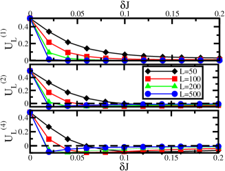
Figure 2: Binder cumulants $U_{L}^{(n)}$ approximated to different orders ($\mathcal{O}(L^{-2n}$)) for the one-dimensional SSH model (Eq. (60)). The phase transition point occurs at $\delta J=0$. The different curves in each panel are for different system sizes $L=50,100,200,500$.

To construct a GBC, first the fourth moment of the polarization is needed, which according to Eq. (3) is the fourth finite difference derivative of the characteristic function,

$$\tilde{M}_{4}^{(1)}=\frac{L^{4}}{(2\pi)^{4}}(2|Z_{2}|-8|Z_{1}|+6).$$ (55)

The Binder cumulant can be written as

$$U_{L}^{(1)}=1-\frac{\tilde{M}_{4}^{(1)}}{3[\tilde{M}_{2}^{(1)}]^{2}}.$$ (56)

This quantity is essentially the same as the $U_{4}$ defined in Eq. (14), albeit here it is introduced in the context of MTP. In general, the quantity $U_{L}^{(m)}$ for any $m$ is size independent by construction, since $Z_{q}=0$ for $q\neq 0$. In Eq. (56) the subscript represents the system size, $L$, the superscript represents the order of approximation used in calculating the moments on the right hand side of the equation. $U_{L}^{(1)}$ is known as a fourth order Binder cumulant (because of the presence of $\tilde{M}_{4}^{(1)}$). Since in Eq. (56) it is the moments which are expressed in terms of a finite difference derivative, we will refer to this way of calculating $U_{L}^{(1)}$ as the moment based approximation (MBA).

Below we make comparisons between the GBC ($U_{L}^{(1)}$) calculated based on the MBA and based on the Resta-Sorella approach, which amounts to taking the finite difference derivative of $\ln Z_{q}$. For the fourth cumulant, the Resta-Sorella approach (up to $\mathcal{O}\left(L^{-2}\right)$) gives

$$C_{4}^{(RS1)}=\frac{L^{4}}{8\pi^{4}}\left[\mbox{Re}\ln Z_{2}-4\mbox{Re}\ln Z_{1}\right].$$ (57)

Using this, we can write the $\mathcal{O}\left(L^{-2}\right)$ approximation to the fourth order GBC as

$$U_{L}^{(RS1)}=-\frac{C_{4}^{(RS1)}}{3[C_{2}^{(RS1)}]^{2}}.$$ (58)

Binder cumulants correct up to higher orders can be constructed using higher order finite difference derivatives.

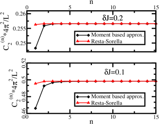
Figure 3: Variance as a function of the order of approximation, $n$, one-dimensional SSH model (Eq. (60)), two cases, $\delta J=0.2$, and $\delta J=0.1$ calculated via two methods: the Resta-Sorella approximation, and the moment based approximation (MBA) developed in this work.

VI Approximating gap closure

In this section we investigate how the MBA expressions for the variance and the GBC behave in the absence of an energy gap. We recall that when the gap is open the GBC is zero (in the thermodynamic limit, which is the same as $\delta t\rightarrow 0$ in Eq. (29)), however, finite values result in closed gap regions. Since our expressions are finite difference approximations, the question that arises is what can we expect at approximations of higher order?

We have shown above that at gap closure $Z_{q}=0$, except for $Z_{0}=1$. We can obtain higher order approximations of the variance by taking higher order finite difference approximations to the second derivative. The variance for the first two orders of approximation are given in Eqs. (53) and (54) ($\mathcal{O}\left(L^{-2}\right)$ and $\mathcal{O}\left(L^{-4}\right)$, respectively). In general, the variance will have the form

$$C_{2}^{(n)}=A_{n}\frac{L^{2}}{4\pi^{2}},$$ (59)

where $A_{n}$ depends on the order of the approximation. For $n=2$, $A_{n}=\frac{5}{2}$ (compare with Eq. (54)). For $n$ up to 30, the value of $A_{n}$ is shown in Fig. 1. The parameter $A_{n}$ appears to converge as a function of $n$. We can estimate a lower bound of $A_{30}=3.224$ for $A_{\infty}$.

The crucial point is that while the value of the variance varies with level of approximation, the scaling with system size within MBA is always two. This also holds for higher order cumulants. For the GBCs, this means that while the value of the GBC at gap closure points will vary as a function of the order of approximation, a GBC of a given approximation will still be size independent at gap closure points. In this sense, the GBCs at a given level of approximation are universal.

The lower panel of Fig. 1 shows the GBC as a function of the order of the approximation, $n$. The value of the cumulant varies considerably as a function of approximation, it decreases as $n$ is increased. The curve appears to level off to a constant value. Locating quantum phase transition points is possible at any order of approximation, since size independence of the GBC is still guaranteed.

VII Model calculations

VII.1 One-dimensional Su-Schrieffer-Heeger model

The Hamiltonian of the Su-Schrieffer-Heeger model Su79 is given by,

$$\hat{H}=\sum_{i=1}^{L}(-Jc_{i}^{\dagger}d_{i}-J^{\prime}d_{i}^{\dagger}c_{i+1}+\mbox{H.c.}),$$ (60)

where $c_{i}^{\dagger}$($d_{i}^{\dagger}$) denote creation operators in one unit cell $i$ on sublattice $A$($B$). This model already has a long history, here we emphasize that it is insulating for $J^{\prime}\neq J$, and gap closure occurs at $J^{\prime}=J$. For convenience we will use the parametrization $J=\bar{J}+\delta J$, $J^{\prime}=\bar{J}-\delta J$, hence, the gap closure occurs at $\delta J=0$. We will take $\bar{J}=1$.

Fig. 2 shows the Binder cumulant based on approximations of different order ($n=1,2,4$) for different system sizes for the 1D SSH model near the gap closure point. Indeed, the Binder cumulants are independent of system size at the phase transition point, however, they exhibit considerable size dependence away from it.

In Fig. 3 the normalized variance is shown as a function of the order of approximation for the two cases ($\delta J=0.1$ and $\delta J=0.2$) for both the MBA, and the Resta-Sorella type approximation carried to higher orders. While, for the gapless case (Fig. 1) the approximation is crucial to obtain quantitative results, for the gapped system the convergence is rapid, a calculation correct up to order $\mathcal{O}\left(L^{-8}\right)$ ($n=4$) is already converged. It is to be noted, however, that the usual Resta-Sorella calculation does give faster convergence as a function of approximation. Still, due to the logarithm, at gap closure points it is undefined, so size scaling information is lost.

While the variance at order $\mathcal{O}\left(L^{-2}\right)$ is not necessarily converged, phase transition points will still be detected, because the GBCs are size independent at each level of finite difference approximation. At $n=1$ ($\mathcal{O}\left(L^{-2}\right)$), the universal value of the GBC at gap closure is $\frac{1}{2}$, as $n$ is increased, the values will be differ, according to Fig. 1 (lower panel). Increasing the order of the finite difference approximation is only important if accurate variance, skew, kurtosis, etc. is desired.

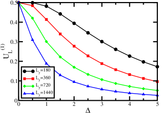
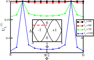
Figure 4: Geometric Binder cumulants for two-dimensional models. Upper panel shows the results for a tight-binding model with an on-site potential (strength $\Delta$) on a square lattice, the middle panel shows the results for a tight-binding model with an on-site potential (strength $\Delta$) on a hexagonal lattice, the lower panel shows results for the topological Haldane model on a hexagonal lattice.

VII.2 Two dimensional models

In two dimensions we consider two different cases of gap closure. For the most basic case (square lattice, tight-binding) gap closure occurs at points along a closed curve within the Brillouin zone. Gap opening can be achieved, for example, by an alternating on-site potential. If the same system is placed on a honeycomb lattice, the gap closure occurs only at isolated points in the Brillouin zone (Dirac points).

For the square lattice, we take the Hamiltonian to consist of nearest neighbor hopping and an on-site potential of strength $\Delta$,

$$\hat{V}=\Delta\sum_{j,k}(-1)^{j+k}\hat{n}_{j,k}.$$ (61)

In reciprocal space the model can be written as:

$$\hat{H}=\sum_{k_{x},k_{y}}\left[\epsilon(k_{x},k_{y})\sigma_{x}+\Delta\sigma_{z}\right],$$ (62)

where

$$\epsilon(k_{x},k_{y})=-2\cos(k_{x})-2\cos(k_{y}),$$ (63)

and where $\sigma_{x}$ and $\sigma_{z}$ denote Pauli matrices. The tight-binding hopping parameter was taken to be unity. We take the basis vectors of the lattice (which give the positions of the $A$ sublattice) to be,

$$\vec{\bf a}_{1}=(2,0);\vec{\bf a}_{2}=(1,1),$$ (64)

leading to a two-dimensional $k$-space grid of

$$k_{x}=\frac{\pi}{L_{x}}m_{x},k_{y}=\frac{2\pi}{L_{y}}m_{y}-\frac{\pi}{L_{x}}m_{x},$$ (65)

with $m_{x},m_{y}=0,...,L-1$. We define the two-dimensional polarization amplitude as

$$Z_{q}=\prod_{m_{x},m_{y}}\langle m_{x},m_{y}|m_{x},m_{y}+q\rangle,$$ (66)

where $|m_{x},m_{y}\rangle$ is an eigenstate of $\epsilon(k_{x},k_{y}){\bf\sigma_{x}}+\Delta{\bf\sigma_{z}}$. Using $Z_{q}$ we can calculate GBCs as given in Eqs. (53), (55), and (56).

The upper panel of Fig. 4 shows the GBC for different system sizes. The lattice size was held fixed in the $x$-direction ($L_{x}=180$), and scaling was done only in the $y$-direction, as indicated by the different $L_{y}$ values in the figure. At the gap closure point, all GBCs converge to their calculated value of $\frac{1}{2}$, away from this point they exhibit size dependence, and decrease monotonically.

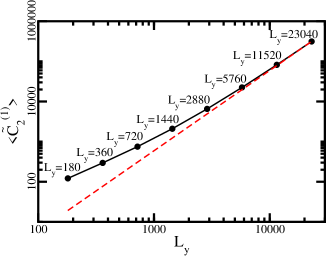
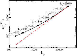
Figure 5: Variance for the hexagonal lattice (upper panel), and the Haldane model (lower panel), both at gap closure, averaged in the transverse direction, shown on a log-log plot. For all calculations $L_{x}$ is held fixed, and $L_{y}$ is varied. The values of $L_{y}$ are shown above each data point. The straight dashed line is the log-log plot of a curve of the form $f(L_{y})=aL_{y}^{2}$. For the hexagonal model (upper panel) $a=0.000593473$, for the Haldane model (lower panel) $a=0.000325063$.

We apply exactly the above procedure for the hexagonal lattice with an alternating on-site potential. In this case, the Hamiltonian takes the form,

$$H=\left[{\begin{array}[]{cc}\Delta&f\\ f^{*}&-\Delta\\ \end{array}}\right].$$ (67)

where

$$f=\exp\left(i\frac{k_{y}}{\sqrt{3}}\right)+2\cos\left(\frac{k_{x}}{2}\right)\exp\left(-i\frac{k_{y}}{2\sqrt{3}}\right).$$ (68)

The coordinate system we use is shown in the inset of the middle panel of Fig. 4. The equilateral triangle connecting second nearest neighbors has sides of length unity. The main figure of the middle panel of Fig. 4 shows the GBCs for the hexagonal lattice. Again, in the gapped region ($\Delta>0$) the GBCs are size dependent, at the gap closure point, ($\Delta=0$) all the GBCs converge to a value of $\frac{1}{2}$.

For completeness we also investigated the topological Haldane model Haldane88 ; Thonhauser06 . In this model, in addition to the on-site potential (which breaks inversion symmetry), a time-reversal symmetry breaking term is also added, consisting of a magnetic flux which encircles the center of each hexagon in such a ways that the Peierls phases ($\Phi$) of the flux only affect the second nearest neighbor hoppings. The tuning of the on-site potential and phase on second nearest neighbor hoppings renders possible the independent control (opening or closing) of each Dirac point separately. The Hamiltonian now has the form,

$$H=\left[{\begin{array}[]{cc}g&f\\ f^{*}&-g\\ \end{array}}\right],$$ (69)

with

$$g=\Delta+2t_{2}\sin(\Phi)\left[\sin(k_{x})+2\sin\left(\frac{k_{x}}{2}\right)\cos\left(\frac{\sqrt{3}k_{x}}{2}\right)\right].$$ (70)

The lower panel of Fig. 4 shows our results for the Haldane model. The inset of the lower panel shows the phase diagram of the model (solid line), and the dashed line indicates the line along which the GBCs were calculated. The main figure of the lower panel shows the GBCs themselves. Two phase transition points are encountered, where the GBCs all take a value of $\frac{1}{2}$. In between and outside the phase transition points, the GBCs are strongly size dependent.

The Fermi surface of the square lattice and the honeycomb lattice are different, the former is a closed one-dimensional curve (a square in the Brillouin zone), the latter is zero-dimensional (two Dirac points). An interesting question is whether finite size scaling methods can distinguish between the two. The quantity capable of doing this is the variance of the polarization averaged in the transverse direction. We define:

$$\langle\tilde{C}_{2}^{(1)}\rangle=\frac{1}{L_{x}}\sum_{k_{x}}\tilde{C}_{2}(k_{x}),$$ (71)

where $C_{2}(k_{x})$ is the variance of the polarization in the $y$-direction for a fixed value of $k_{x}$ (according to the definition in Eq. (53)). Of particular interest is the scaling of $\langle C_{2}^{(1)}\rangle$ as a function of system size. We approximate

$$\langle\tilde{C}_{2}^{(1)}\rangle=aL^{\gamma},$$ (72)

where $a$ is a coefficient, and $\gamma$ is the size scaling exponent. For the square lattice, when the system size is scaled both in the $x$ and $y$ directions simultaneously, the size scaling exponent $\gamma=2$ at the gap closure point, and $\gamma=1$ for gapped systems. We checked this via calculations for system sizes of $L_{x}=L_{y}=180\times 2^{k}$, $k=0,1,2,3,4,5,6,7$. For the hexagonal lattice, based on calculations of the same set of system sizes, when scaling is done in both directions $\gamma\approx 1.12$ for the gapless case, while $\gamma=1$ for gapped systems. However, if scaling is only done in one dimension, then for large system sizes the scaling exponent becomes $\gamma=2$ for the gapless case (for the gapped systems it still holds that $\gamma=1$). The results are shown in Fig. 5. For $L_{x}=180$ fixed, as $L_{y}$ is varied, the log-log plot for the average variance as a function of system size does not show a straight line, however, as $L_{y}$ becomes large, the function does tend to a curve with $L_{y}$ dependence $L_{y}^{2}$, hence $\gamma=2$. The different panels of Fig. 5 correspond to the different hexagonal models: upper panel(lower panel) shows the honeycomb tight-binding(Haldane) model.

These results can be explained from the form of Eq. (71). For a two-dimensional system whose Fermi surface is a closed curve which runs over the entire Brillouin zone, a gap closure point will be encountered for each $k_{x}$, which will render $Z_{1}$ zero, and lead to a contribution to $\langle C_{2}^{(1)}\rangle$ with a scaling exponent of $\gamma=2$. For a system with Dirac points, the contributions to $\langle C_{2}^{(1)}\rangle$ scale as $L_{y}$, except for values of $k_{x}$, which encounter Dirac points, which scale as $L_{y}^{2}$. In this case $L_{y}$ has to be increased so that this one term dominates the scaling of $\langle C_{2}^{(1)}\rangle$.

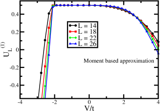
Figure 6: Binder cumulant for the $t-V$ one-dimesional interacting model, as a function of $V/t$. The upper panel shows results for the Resta-Sorella approximation, the lower one for the moment based approximation.

VII.3 Correlated one-dimensional model

Our last model calculation is the $t-V$ model, a one-dimensional tight-binding model (hopping $t$) with nearest neighbor interaction $V$. The Hamiltonian is given by

$$H=\sum_{i=1}^{L}\left[-t(c_{i}^{\dagger}c_{i+1}+c_{i+1}^{\dagger}c_{i})+Vn_{i}n_{i+1}\right].$$ (73)

This model exhibits phase transitions at $V=\pm 2t$. If $|V|<2t$ the system is in a gapless Luttinger liquid phase, whereas, $|V|>2t$ is an insulating phase. The phase transition at $V=2t$ is second order, while the one at $V=-2t$ is first order. We perform exact diagonalization calculations (Lánczos method).

System sizes	Repulsive fixed point	Repulsive fixed point
$L=16/8$	$V=3.00t$	$V=-2.21t$
$L=20/10$	$V=2.75t$	$V=-2.13t$
$L=24/12$	$V=2.62t$	$V=-2.08t$
$L=28/14$	$V=2.52t$	$V=-2.06t$

Table 2: The repulsive fixed points for the $t-V$ model for different pairs of system sizes.

In Fig. 6 the Binder cumulant is shown for a sweep across both phase transitions for different system sizes. The upper panel shows results for the Resta-Sorella approximation (the $V=0$ is missing, since there the logarithms give a divergent result), the lower for MBA. In both cases the first-order phase transition is easy to identify. Overall, it is difficult to say whether the Resta-Sorella method converges to a precise value in the gapless phase, since even there there is some size dependence, and the value of the cumulant is difficult to identify. In the MBA, the cumulants converge in the region $-2t<V<2t$ to a value of one half, and the phase transition at $V=-2t$ is clearly identifiable. As for the second order phase transition at $V=2t$, the MBA is superior to the Resta-Sorella approach, partly because the Resta-Sorella method does not converge to a universal value in the gapless phase.

Another striking feature of the results in Fig. 6 is that in the ordered phases $V>|2t|$ the Binder cumulant is not zero. This is due to the fact that in the many-body case the polarization is not a usual Berry-Zak phase (integral across the Brillouin zone), it is, instead, a single point Resta00 Berry phase. One can calculate $Z_{q}$ in the ordered phases (see Ref. Hetenyi19 ), and one obtains a Binder cumulant of minus infinity. Still, the gap closure region is easily identified.

For comparison, we also used another method to locate the phase transition point. This method is an application of real-space renormalization to the polarization amplitude Hetenyi21 . For a given value of $V$, $Z_{1}$ is calculated for some initial system size $L$. Then for $L/2$ the value of $V$ is tuned to reproduce the same $Z_{1}$ as for the larger system. This generates a renormalization trajectory, via

$$Z_{1}(V_{j+1},L/2)=Z_{1}(V_{j},L),$$ (74)

and fixed points as a function of $V$ can be determined. The trajectories tend to an attractive fixed points at $V=0$, $V=\infty$, and $V=-\infty$, and two repulsive fixed points occur at finite $V$ in between the three attractive fixed points. The repulsive fixed points correspond to the phase transition points. Our calculated results for the repulsive fixed points are shown in table 2. Again, the phase transition point in the attractive region of the model ($V<0$) is easy to locate, our best result being $V=-2.06t$. In the region $V>0$, for the largest system size we are able to do, the repulsive fixed point is at $V\approx 2.52$, in good agreement with our results in the lower panel of Fig. 6. We emphasize that the limitation is not the finite size scaling methods advocated here, but the system size accessible by exact diagonalization.

VIII Conclusion and Future Prospects

In this work we explored a generalization of the study of adiabatic cycles initiated in the context of quantum mechanics by Berry Berry84 . A geometric phase becomes non-trivial if the adiabatic cycle over which it is defined encircles a degeneacy point. If the path is modified so that it crosses the degeneracy point, the Berry phase becomes undefined. The direction of our generalization was the consideration of cycles which cross isolated degeneracy points. We showed that it is possible to define quantities which are physically well defined in this case. The quantities which achieve the above goal are ratios of the cumulants associated with adiabatic cycles. We gave a detailed analysis of how cumulant generating functions can be defined in the general context of the geometric phase, as well as the particular context of the modern theory of polarization. For the latter we drew on the work of Souza, Wilkens, and Martin  Souza00 .

In the modern polarization context we defined cumulant ratios which we showed to be useful for finite size scaling of quantum phase transitions. We argued that the method often used in the literature, due to Resta and Sorella Resta98 ; Resta99 , has a drawback, namely that the size scaling of the variance of the polarization is lost at the phase transition points. We presented an alternative approximation scheme which leads to controlled divergence of the system size at phase transition point. The geometric Binder cumulants we derived are ratios of cumulants of the polarization defined according to our approximation scheme.

We also presented numerical model calculations of the techniques developed. The geometric Binder cumulant can detect the gap closure in all cases studied, which included one-dimensional and two-dimensional band models, and a one-dimensional correlated system.

In two dimensions we investigated two different types of gap closures. Some models exhibit one-dimensional Fermi surfaces (for example, a simple two-dimensional tight-binding model. Other models, such as graphene, or the topological Haldane model, exhibit isolated points as Fermi surfaces (Dirac points). We showed that the geometric Binder cumulant detects gap closure in both cases, provided, that scaling is done in one dimension only. We also showed that the variance, if system size scaling is done in two directions, will not detect the gap closure in the case of models with Dirac points, because, even though for one particular $k$-vector the gap closure does indeed cause a divergence, this effect is statistically suppressed by the presence other $k$-vectors. Scaling in one direction solves this problem.

The geometric phase has by now a considerable history, and many generalizations have been done. One well-known extension Wilczek84 is the application to systems in which degeneracies originating from symmetry exist, for example, if time-reversal symmetry leads to Kramers doublets AldenMead87 . In this case the integral defining the geometric phase becomes the Wilson loop, and the geometric phase itself becomes an $SU(2)$ matrix (a quaternion). The adiabatic loop is of particular interest if it encircles crossing points between Kramers doublets. We are confident that our ideas are applicable to these types of more complex scenarios.

References

- (1) M. V. Berry, Proc. Roy. Soc. London A392 45 (1984).
- (2) I. Souza, T. Wilkens, and R. M. Martin, Phys. Rev. B 62 1666 (2000).
- (3) M. Imada, A. Fujimori, and Y. Tokura, Rev. Mod. Phys. 70 1039 (1998).
- (4) J. Zak, Phys. Rev. 62 2747 (1989).
- (5) R. D. King-Smith and D. Vanderbilt, Phys. Rev. B 47 R1651 (1993).
- (6) R. Resta, Rev. Mod. Phys. 66 899 (1994).
- (7) R. Resta, J. Phys.: Cond. Mat. 12 R107 (2000).
- (8) D. Vanderbilt, Berry Phases in Electronic Structure Theory, Cambridge University Press, Cambridge, U.K. (2018).
- (9) W. Kohn, Phys. Rev. 133, A171 (1964).
- (10) E. K. Kudinov, Fiz. Tverd. Tela 33 2306 (1991) [Sov. Phys. Solid State 33, 1299 (1991)].
- (11) N. Marzari and D. Vanderbilt, Phys. Rev. B 56 12847 (1997).
- (12) N. Marzari, A. A. Mostofi, J. R. Yates, I. Souza and D. Vanderbilt, Rev. Mod. Phys. 84 1419 (2012).
- (13) H. Watanabe and M. Oshikawa, Phys. Rev. X 8 021065 (2018).
- (14) M. Yahyavi and B. Hetényi, Phys. Rev. A 95 062104 (2017).
- (15) R. Resta and S. Sorella, Phys. Rev. Lett. 82 370 (1999).
- (16) S. Patankar, L. Wu, B. Lu, M. Rai, J. D. Tran, T. Morimoto, D. E. Parker, A. G. Grushin, N. L. Nair, J. G. Analytis, J. E. Moore, J. Orenstein, and D. H. Torchinsky, Phys. Rev. B 98 165113 (2018).
- (17) W. P. Su, J. R. Schrieffer and A. J. Heeger, Phys. Rev. Lett. 42 1698 (1979).
- (18) B. A. Bernevig and T. L. Hughes, Topological Insulators and Superconductors, Princeton University Press (2013).
- (19) F. D. M. Haldane, Phys. Rev. Lett. 61 2015 (1988).
- (20) C. L. Kane, in Topological Insulators, vol. 6 Eds. M. Franz and L. Molenkamp, Chapter 1, Elsevier (2013).
- (21) C. L. Kane and E. J. Mele, Phys. Rev. Lett. 95 226801 (2005).
- (22) C. L. Kane and E. J. Mele, Phys. Rev. Lett. 95 146802 (2005).
- (23) T. Thonhauser and D. Vanderbilt, Phys. Rev. B 74 235111 (2006).
- (24) M. E. Fisher, in Critical Phenomena, Proc. 51st Enrico Fermi Summer School, Varena, edited by M. S. Green (Academic Press, N.Y.) 1972.
- (25) M. E. Fisher and M. N. Barber, Phys. Rev. Lett. 28 1516 (1972).
- (26) K. Binder, Z. Phys. B 43 119 (1981).
- (27) K. Binder, Phys. Rev. Lett. 47 693 (1981).
- (28) V. Bargmann, J. Math. Phys. 5 862 (1964).
- (29) F. B. Hildebrand, Finite-Difference Equations and Simulations,Prentice-Hall, Englewood Cliffs, New Jersey (1968).
- (30) W. Selke, Eur. Phys. J. B 51 223 (2006).
- (31) B. Hetényi, M. H. Müser, and B. J. Berne, Phys. Rev. Lett. 83 4606 (1999).
- (32) M. Born and V. Fock, Z. für Phys. 51 165 (1928).
- (33) T. Kato, J. Phys. Soc. Jpn. 5 485 (1950).
- (34) R. Resta, Phys. Rev. Lett. 80 1800 (1998).
- (35) B. Hetényi and B. Dóra, Phys. Rev. B 99 085126 (2019).
- (36) B. Hetényi, Phys. Rev. Research 2 023277 (2020).
- (37) G. Chiappe, E. Louis, and J. A. Vergés, J. Phys.: Condens. Matter 30 175603 (2018).
- (38) B. Hetényi, S. Parlak, and M. Yahyavi, Phys. Rev. B 104 214207 (2021).
- (39) F. Wilczek and A. Zee, Phys. Rev. Lett. 52 2111 (1984).
- (40) C. A. Mead, Phys. Rev. Lett. 59 161 (1987).