Different routes to the classical limit of backflow

Abstract

Decoherence is a well established process for the emergence of classical mechanics in open quantum systems. However, it can have two different origins or mechanisms depending on the dynamics one is considering, speaking then about intrinsic decoherence for isolated systems and environmental decoherence due to dissipation/fluctuations for open systems. This second mechanism can not be considered for backflow since no thermal fluctuation terms can be added in the formalism in order to keep an important requirement for the occurrence of this effect: only contributions of positive momenta along time should be maintained. The purpose of this work is to analyze the backflow effect in the light of the underlying intrinsic decoherence and the dissipative dynamics. For this goal, we first deal with the Milburn approach where a mean frequency of the unitary evolution steps undergone for the system is assumed. A comparative analysis is carried out in terms of the Lindblad master equation. Second, the so-called quantum-to-classical transition wave equation is analyzed from a linear scaled Schrödinger equation which is derived and expressed in terms of a continuous parameter covering from the quantum to the classical regime as well as all in-between dynamical non-classical regimes. This theoretical analysis is inspired by the Wentzel-Kramers-Brillouin approximation. And third, in order to complete our analysis, the transition wave equation formalism is also applied to dissipative backflow within the Caldirola-Kanai approach where the dissipative dynamics comes from an effective Hamiltonian. In all the cases treated here, backflow is gradually suppressed as the intrinsic decoherence process is developing, paying a special attention to the classical limit. The route to classicality is not unique.

• October 2022

Keywords: Backflow, classical limit, intrinsic decoherence, transition wave equation, dissipative dynamics, Lindblad equation

1 Introduction

Backflow is usually referred when free particles described by a one-dimensional wave function consisting of a distribution of positive momenta along time, display an increasing probability of remaining in the negative region during certain periods of time (backflow intervals). This counter-intuitive quantum phenomenon was initially noticed by Allock [1] in his study of arrival times in quantum mechanics. A detailed study of the problem was only carried out 25 years later by Bracken and Melloy [2] where they introduced a new quantum number, today known as the Bracken-Melloy constant, being independent on the backflow interval, particle mass and Planck constant. This value was computed numerically to be around 0.04 and is the least upper bound for backflow i.e., the greatest amount of probability for flowing from right to left through the origin. Furthermore, it appears to be the largest eigenvalue of a homogeneous Fredholm integral equation of second kind. Some rigorous results about the backflow operator have been derived elsewhere [3].

This effect has also been studied in the presence of a constant force [4] and extended to the realm of relativistic quantum mechanics [5, 6, 7, 8]. Its connection to arrival times [9, 10], diffraction in time [11] and quantum reentry [12] have been considered. In this regard, it has been demonstrated that construction of correlated quantum states for which the amount of backflow can exceed the Bracken-Melloy constant is possible [12]. More recently, a new formulation of the quantum backflow problem for arbitrary momentum distributions has been proposed and applied for gravitational and harmonic potentials [13, 14]. Moreover, backflow has been considered for the rotational motion [15, 16, 17, 18] and has been addressed in connection with nonclassicality and the Wigner function [19]. Studies of quantum backflow have also been extended to open quantum systems within the Caldirola-Kanai (CK) framework [20] as well as for identical particles [21]. A general formulation of quantum backflow for conservative systems of free non-relativistic many particles, both distinguishable and identical, has been carried out [22]. While experimental evidences for this effect have not been reported yet, its optical counterpart has recently been observed [23].

Decoherence or the emergence of classical properties in a given physical system is usually considered in the context of open quantum dynamics where the environment is entangled with the system of interest. This kind of decoherence is usually called external or environmental decoherence [24, 25]. Just in the opposite side it is found in the literature what is known as intrinsic decoherence which is intrinsic to Nature itself (it is ineluctable) and where no environment is involved [26, 25] and, therefore, it can even exist for an isolated system. Over the years, several different paths have been taken to break up with the standard quantum mechanics; some of the well-known attempts include the postulation of extra nonlinear terms or stochastic terms in the Schrödinger equation; and gravitational effects invalidates this equation [25]. Several years ago, Milburn [26] postulated that, at sufficiently short time steps, the system does not evolve continuously under unitary evolution but by a stochastic sequence of identical unitary transformations. This means that a minimum time step in the universe is introduced. The inverse of this time step is the mean frequency of the unitary steps. The system is then considered isolated and described by a state whose evolution is governed by a generalized von Neumann equation having this mean frequency as a parameter.

In this work, we also propose an additional intrinsic decoherence inspired by the Wentzel-Kramers-Brillouin (WKB) approximation. In an attempt to describe both the quantum and classical regimes in a uniform language and continuous way, a non-linear wave equation has been proposed for such a transition [27]. It has been then proved that this non-linear equation is equivalent to a linear one which is just a Schrödinger equation but with a scaled Planck constant and scaled wave function [28, 29]. This transition wave equation contains a parameter ranging from one (quantum regime) to zero (classical regime) covering all the regimes in-between (non-classical dynamical regimes) which is equivalent to consider the limit $\hbar\rightarrow 0$. The procedure of using a continuous parameter monitoring the different dynamical regimes in the theory could be seen quite similar to the WKB approximation (based on a series expansion in powers of Planck constant), widely used for conservative systems in the energy domain. However, some important differences should be clearly stressed. First, whereas the classical Hamilton-Jacobi equation for the action is obtained at zero order in the WKB approximation, the so-called classical time-dependent (non-linear) wave equation [30] is reached by construction. Second, the hierarchy of the differential equations for the action at different orders of the expansion in $\hbar$ is substituted by a transition wave differential equation which can be solved in the linear and non-linear domains. Third, the transition from quantum to classical trajectories is carried out in a continuous and gradual way, covering all the intermediate non-classical dynamical regimes. Fourth, the scaling procedure extended and applied to open quantum systems is very easy to implement. And fifth, the gradual (intrinsic) decoherence process due to the scaled Planck constant allows us to analyze the continuity of the intermediate dynamical regimes to finally reach the classical regime. At this level, it is interesting to point out that this process studied within this theoretical scheme displays decoherence due to the gradual transition from the quantum to the classical regime. This kind of studies has been extended to dissipative and stochastic dynamics in the framework of the CK and the so-called Schrödinger-Langevin or Kostin equations, respectively [28, 29, 31].

Finally, an interesting aspect deserving special attention is the classical limit of the backflow effect; in particular, because of the independence of the Bracken-Melloy constant from the Planck constant, this limit cannot be taken naively. An attempt has already been carried out by Yearsley et al. [32, 9] using quasi-projectors in the definition of the flux operator. Recently, Bracken [33] has proposed another way for treating the classical limit of backflow by generalizing the eigenvalue problem where the allowed range of momentum values is expanded beyond those previously considered. In this work, our purpose is also to consider this goal by analyzing it in terms of the intrinsic decoherence and dissipative dynamics. Such a study in the direction of the classical limit of backflow via the scaled Schrödinger equation confirms that backflow is a non-classical effect in the sense that it is not observed in systems of classical particles. However, it should be noted that this effect is a wave phenomenon which can be seen for classical waves too [8]. This is due to the fact that the wave-particle duality is absent in classical mechanics. The situation is similar to quantum tunneling but in classical optics; frustrated total reflection [34]. Two particular problems will be analyzed, the Bracken and Melloy classical example both for non-dissipative and dissipative dynamics is studied and the free propagation of a superposition of two Gaussian wave packets. In all of these cases, backflow is gradually suppressed as the intrinsic decoherence process is developing and the classical limit is reached.

2 Backflow within the von Neumann formalism

In the most general formulation of quantum mechanics, a physical system is described by a density operator $\hat{\rho}$ instead of a state vector $|\psi\rangle$. In this context, the von Neumann equation

$$i\hbar\frac{\partial\hat{\rho}}{\partial t} = [\hat{H},\hat{\rho}]$$ (1)

has to be applied for the time evolution of the system, $\hat{H}$ being the Hamiltonian of the system. For a single particle and in one dimension, this Hamiltonian is expressed as

$$\hat{H} = \frac{\hat{p}^{2}}{2m}+V(\hat{x}),$$ (2)

where the first term is the kinetic energy operator and the second term, the external interaction potential. We are interested in backflow for free particles. For this goal, the Hamiltonian is reduced to the first term describing the kinetic energy of free particles.

In the momentum representation, the von Neumann equation (1) for free particles is written as

$$i\hbar\frac{\partial}{\partial t}\rho(p,p^{\prime},t) = \frac{p^{2}-p^{\prime 2}}{2m}\rho(p,p^{\prime},t),$$ (3)

its solution being

$$\rho(p,p^{\prime},t) = \exp\left[-\frac{i}{\hbar}\frac{p^{2}-p^{\prime 2}}{2m}t\right]\rho(p,p^{\prime},0).$$ (4)

On the contrary, in the position representation, Eq. (1) is expressed as

$$i\hbar\frac{\partial}{\partial t}\varrho(x,x^{\prime},t) = -\frac{\hbar^{2}}{2m}\left(\frac{\partial^{2}}{\partial x^{2}}-\frac{\partial^{2}}{\partial x^{\prime 2}}\right)\varrho(x,x^{\prime},t),$$ (5)

which, in terms of the center of mass and relative coordinates, $R=(x+x^{\prime})/2$ and $r=x-x^{\prime}$, it can be rewritten as

$$\frac{\partial}{\partial t}\varrho(R,r,t)+\frac{\partial}{\partial R}j(R,r,t) = 0,$$ (6)

where we have introduced the probability current density matrix

$$j(R,r,t) = \frac{\hbar}{im}\frac{\partial}{\partial r}\varrho(R,r,t).$$ (7)

Diagonal elements are obtained from $r=0$ and $R=x$, $\varrho(x,t)=\varrho(R=x,r=0,t)$ and $j(x,t)=j(R=x,r=0,t)$ being then the probability density and probability current density fulfilling the continuity equation

$$\frac{\partial}{\partial t}\varrho(x,t)+\frac{\partial}{\partial x}j(x,t) = 0.$$ (8)

From the continuity equation (8), one has, after integration over $x$ between $-\infty$ and $0$, that

$$\frac{d}{dt}\mbox{Pr}(t) = -j(0,t),$$ (9)

where $\mbox{Pr}(t)$ gives the probability of finding the particle in the negative half-space, $x<0$; we have assumed that $j(-\infty,t)=0$. Except if $j(0,t)$ is negative, $\mbox{Pr}(t)$ is a decreasing function of time. If $j(0,0)$ is negative then, by continuity in time, $j(0,t)$ will be negative over some time interval, say $[0,t_{b})$ [2]. Then, from Eq. (9), the increasing probability or transmitted right-to-left probability in this time interval is given by

$${\Delta}_{t_{b}} = \mbox{Pr}(t_{b})-\mbox{Pr}(0)=-\int_{0}^{t_{b}}dt~{}j(0,t)=\int_{0}^{t_{b}}dt~{}j_{{}_{-}}(0,t),$$ (10)

where in the last equality we have used the negativity of $j$ in the interval $[0,t_{b})$ and introduced

$$j_{{}_{-}}(0,t) = \frac{|j(0,t)|-j(0,t)}{2}.$$ (11)

If the contribution of negative momenta to the probability density at all times is zero, then one speaks of backflow and the interval $[0,t_{b})$ is called the backflow time interval.

The density matrix in the position representation written in terms of its elements in the momentum space are computed from

$$\varrho(x,x^{\prime},t) = \langle x|\hat{\rho}(t)|x^{\prime}\rangle=\int_{-\infty}^{\infty}dp\int_{-\infty}^{\infty}dp^{\prime}\langle x|p\rangle\langle p|\hat{\rho}(t)|p^{\prime}\rangle\langle p^{\prime}|x^{\prime}\rangle$$ (12)

$$= \frac{1}{2\pi\hbar}\int_{-\infty}^{\infty}dp\int_{-\infty}^{\infty}dp^{\prime}e^{i(px-p^{\prime}x^{\prime})/\hbar}~{}e^{-i(p^{2}-p^{\prime 2})t/2m\hbar}\rho(p,p^{\prime},0),$$

where in the second line we have used Eq. (4). From Eqs. (12) and (53), we have then that

$$j(0,t) = \frac{1}{4m\pi\hbar}\int_{-\infty}^{\infty}dp\int_{-\infty}^{\infty}dp^{\prime}(p+p^{\prime})e^{-i(p^{2}-p^{\prime 2})t/2m\hbar}\rho(p,p^{\prime},0).$$ (13)

For a mixture of states i.e.,

$$\rho(p,p^{\prime},0) = \sum_{i}w_{i}\phi_{i}(p)\phi_{i}^{*}(p^{\prime}),\qquad\sum_{i}w_{i}=1,$$ (14)

$j$ is also a mixture with the same weights $w_{i}$,

$$j(0,t) = \sum_{i}w_{i}j_{i}(0,t),$$ (15)

with

$$j_{i}(0,t) = \frac{1}{4m\pi\hbar}\int_{-\infty}^{\infty}dp\int_{-\infty}^{\infty}dp^{\prime}(p+p^{\prime})e^{-i(p^{2}-p^{\prime 2})t/2m\hbar}\phi_{i}(p)\phi_{i}^{*}(p^{\prime}).$$ (16)

For quantum backflow, only contributions coming from positive momenta will be considered.

As an illustration, let us consider the mixture of two states $\phi_{1}(p)$ and $\phi_{2}(p)$ with weights $w$ and $1-w$, respectively, where

$$\phi_{1}(p) = \frac{18}{\sqrt{35~{}\hbar k}}\frac{p}{\hbar k}\left(e^{-p/\hbar k}-\frac{1}{6}e^{-p/2\hbar k}\right)\Theta(p)$$ (17)

$$\phi_{2}(p) = \sqrt{\frac{2}{\hbar k}}e^{-p/\hbar k}\Theta(p),$$ (18)

$k$ being a positive wave number and $\Theta(p)$ is the Heaviside function. Eq. (17) is the state used by Bracken and Melloy in their first study of backflow [2]. Then, from Eq. (16) we have that

$$j_{1}(0,0) = -\frac{36}{35\pi}\frac{\hbar k^{2}}{m},$$ (19)

$$j_{2}(0,0) = \frac{1}{\pi}\frac{\hbar k^{2}}{m},$$ (20)

$$j(0,0) = wj_{1}(0,0)+(1-w)j_{2}(0,0)=\frac{1}{\pi}\frac{\hbar k^{2}}{m}\left(1-w\frac{71}{35}\right).$$ (21)

These results show that the state $\phi_{1}(p)\phi_{1}^{*}(p^{\prime})$ displays backflow while the state $\phi_{2}(p)\phi_{2}^{*}(p^{\prime})$ does not. Thus, the mixed state $\rho(p,p^{\prime},0)=w\phi_{1}(p)\phi_{1}^{*}(p^{\prime})+(1-w)\phi_{2}(p)\phi_{2}^{*}(p^{\prime})$ displays quantum backflow only when $35/71<w\leq 1$.

3 Backflow in the framework of the Milburn approach

Several years ago, Milburn [26] introduced what is known as intrinsic decoherence in quantum mechanics by postulating that, at sufficiently short time steps, the system does not evolve continuously under unitary evolution but by a stochastic sequence of identical unitary transformations. This means that a minimum time step in the universe should be introduced. The inverse of this time step is the mean frequency of the unitary steps, $\lambda$. In this way, a generalized evolution equation was proposed whose expansion to first order in $\lambda^{-1}$ reads as

$$\frac{\partial\hat{\rho}}{\partial t} = -\frac{i}{\hbar}[\hat{H},\hat{\rho}]-\frac{1}{2\hbar^{2}\lambda}[\hat{H},[\hat{H},\hat{\rho}]].$$ (22)

In the limit $\lambda\rightarrow\infty$, this equation reduces to the von Neumann equation (1). Furthermore, the Milburn equation (22) preserves the trace of the density operator.

In the momentum representation, the Milburn equation (22) for free particles reads as

$$\frac{\partial}{\partial t}\rho(p,p^{\prime},t) = \left[-\frac{i}{\hbar}\frac{p^{2}-p^{\prime 2}}{2m}-\frac{1}{2\hbar^{2}\lambda}\left(\frac{p^{2}-p^{\prime 2}}{2m}\right)^{2}\right]\rho(p,p^{\prime},t),$$ (23)

its solution being

$$\rho(p,p^{\prime},t) = \exp\left[-\frac{i}{\hbar}\frac{p^{2}-p^{\prime 2}}{2m}t-\frac{1}{2\hbar^{2}\lambda}\left(\frac{p^{2}-p^{\prime 2}}{2m}\right)^{2}t\right]\rho(p,p^{\prime},0).$$ (24)

As this solution shows, diagonal elements are constant in time while non-diagonal elements decay exponentially showing the effect of the so-called intrinsic decoherence. For environmental decoherence, within the Caldeira-Leggett formalism, the non-diagonal terms decay with time at a rate governed by the damping constant and temperature [35]. Furthermore, if the initial state contains only positive momenta, the corresponding time evolving state too.

Eq. (22) for free particles in the position representation takes now the form

$$\frac{\partial}{\partial t}\varrho(x,x^{\prime},t) = \left[-\frac{i}{\hbar}-\frac{1}{2\hbar^{2}\lambda}\frac{-\hbar^{2}}{2m}\left(\frac{\partial^{2}}{\partial x^{2}}-\frac{\partial^{2}}{\partial x^{\prime 2}}\right)\right]\frac{-\hbar^{2}}{2m}\left(\frac{\partial^{2}}{\partial x^{2}}-\frac{\partial^{2}}{\partial x^{\prime 2}}\right)\varrho(x,x^{\prime},t).$$

In the $(R,r)$ coordinates, this equation is equivalent to Eq. (6) but with the probability current density matrix given by

$$j(R,r,t) = \left(-\frac{i\hbar}{m}+\frac{\hbar^{2}}{2\lambda m^{2}}\frac{\partial^{2}}{\partial r\partial R}\right)\frac{\partial}{\partial r}\varrho(R,r,t).$$ (26)

The density matrix in the position representation is then given by the inverse Fourier transform of its representation in the momentum space according to

$$\varrho(R,r,t) = \frac{1}{2\pi\hbar}\int_{-\infty}^{\infty}dp\int_{-\infty}^{\infty}dp^{\prime}e^{i(p-p^{\prime})R/\hbar}e^{i(p+p^{\prime})r/2\hbar}\rho(p,p^{\prime},t),$$ (27)

and using Eq. (26) the probability current density is given by

$$j(x,t) = \frac{1}{4\pi m\hbar}\int_{-\infty}^{\infty}dp\int_{-\infty}^{\infty}dp^{\prime}e^{i(p-p^{\prime})x/\hbar}(p+p^{\prime})\left(1-i\frac{p^{2}-p^{\prime 2}}{4\hbar m\lambda}\right)\rho(p,p^{\prime},t),$$

which is a real function due to the fact that $\rho(p,p^{\prime},t)=\rho^{*}(p^{\prime},p,t)$. In order to simplify the notation, one can use some characteristic length $\mu$ and time $\nu=\mu^{2}m/\hbar$ and then represent dimensionless variables by capital letters according to

$$X = \frac{x}{\mu},$$ (29)

$$T = \frac{t}{\nu},$$ (30)

$$P = \mu\frac{p}{\hbar},$$ (31)

and for functions,

$$\Psi(X,T) = \sqrt{\mu}~{}\psi(x,t),$$ (32)

$$\Phi(P,T) = \sqrt{\frac{\hbar}{\mu}}~{}\phi(p,t),$$ (33)

$$J(X,T) = \nu~{}j(x,t).$$ (34)

Thus, one has that

$$J(X,T) = \frac{1}{4\pi}\int_{-\infty}^{\infty}dP\int_{-\infty}^{\infty}dP^{\prime}e^{i(P-P^{\prime})X}(P+P^{\prime})\left(1-i\frac{P^{2}-P^{\prime 2}}{4\Lambda}\right)\bar{\rho}(P,P^{\prime},T),$$

where $\Lambda=\nu\lambda$ and $\bar{\rho}(P,P^{\prime},T)=(\hbar/\mu)~{}\rho(p,p^{\prime},t)$ and

$$J(0,T) = \frac{1}{4\pi}\int dP\int dP^{\prime}(P+P^{\prime})~{}\mbox{Re}\{\bar{\rho}(P,P^{\prime},T)\}$$ (36)

$$+ \frac{1}{16\pi\Lambda}\int dP\int dP^{\prime}(P+P^{\prime})^{2}(P-P^{\prime})~{}\mbox{Im}\{\bar{\rho}(P,P^{\prime},T)\}.$$

Note that the standard quantum mechanics expression is reached when $\Lambda\rightarrow\infty$. Thus, the second term shows the contribution of the intrinsic decoherence in the backflow dynamics.

We now consider two specific examples. As stated previously, for backflow the contribution of negative momenta to the state must be zero and $J(0,0)$ has to be negative.

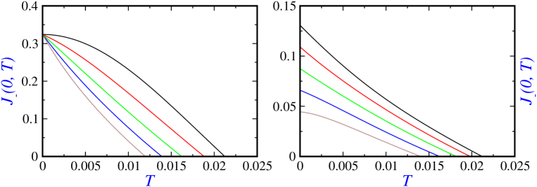
Figure 1: Negative part of the probability current density at the origin for different values of $\Lambda^{-1}$: $\Lambda^{-1}=0$ (black), $\Lambda^{-1}=0.005$ (red), $\Lambda^{-1}=0.01$ (green), $\Lambda^{-1}=0.015$ (blue) and $\Lambda^{-1}=0.02$ (brown) for the initial state given by Eq. (38) (left panel) and Eq. (39) (right panel).

In figure 1, the negative part of the probability current density at the origin, $J_{-}(0,T)$, for different values of $\Lambda$ for a pure state is plotted

$$\bar{\rho}(P,P^{\prime},0) = \Phi(P)\Phi^{*}(P^{\prime})$$ (37)

with the so-called Bracken-Melloy state Eq. (17) (left panel)

$$\Phi(P) = \frac{18}{\sqrt{35}}P\left(e^{-P}-\frac{1}{6}e^{-P/2}\right)\Theta(P)$$ (38)

and a different state (right panel) given by

$$\Phi(P) = \sqrt{\frac{1823508}{253055}}P\left(e^{-(1+i/2)P}-\frac{1}{6}e^{-(1+i/2)P/2}\right)\Theta(P).$$ (39)

Note that dimensionless space and time coordinates are used according to

$$\mu=\frac{1}{k}$$ (40)

$$\nu=\frac{\mu^{2}m}{\hbar}=\frac{m}{\hbar k^{2}}.$$ (41)

In the former case, the contribution of the second term in Eq. (36) is zero initially whereas this is not true in the second case. Because of this, in the right panel, the curves corresponding to different values of $\Lambda$ start initially at different values. As this figure also shows, backflow is suppressed gradually as $\Lambda$ decreases revealing the role of the intrinsic decoherence. Note that both the backflow interval and the amount of backflow are reduced due to this type of decoherence.

In figure 2, the probability current density at the origin is plotted versus time for different values of the parameter $\Lambda^{-1}$ for the superposition of two Gaussian wave packets in the momentum representation

$$\Phi(P) = N\left(\frac{2}{\pi}\right)^{1/4}\left\{e^{-(P-P_{0a})^{2}}+\alpha e^{i\theta}e^{-(P-P_{0b})^{2}}\right\},$$ (42)

where the normalization factor is given by

$$N = \left(1+\alpha^{2}+2\alpha\cos\theta~{}e^{-(P_{0a}-P_{0b})^{2}/2}\right)^{-1/2}.$$ (43)

Here space and time have been expressed in terms of

$$\mu=\frac{\hbar}{2\sigma_{p}}$$ (44)

$$\nu=\frac{\mu^{2}m}{\hbar}=\frac{m\hbar}{4\sigma_{p}^{2}},$$ (45)

$\sigma_{p}$ being width of the component wavepackets. With values $P_{0a}=14$, $P_{0b}=3$, $\alpha=1.9$ and $\theta=\pi$ the contribution of negative momenta to the wave packet is negligible around $10^{-10}$. As clearly seen, for the standard quantum mechanics where $\Lambda^{-1}=0$ (panel a), there are three intervals of backflow while for the remaining three other values (panels b, c and d) only a single backflow interval is seen at very short times. Furthermore, the intrinsic decoherence makes this time interval shorter. This fact is better observed in the left panel of figure 3 where the corresponding negative part is plotted for different values of $\Lambda^{-1}$ and the right bottom panel where the duration of backflow is depicted in terms of $\Lambda^{-1}$. In the right panels of the same figure, the amount of backflow (top) quantified by means of the integral of negative part of the probability current density over the first backflow interval $[0,T_{b})$

$$\Delta_{T_{b}} = \int_{0}^{T_{b}}dt~{}J_{-}(0,t)$$ (46)

and the first backflow duration (bottom) are plotted as a function of $\Lambda^{-1}$. One sees again that the intrinsic decoherence reduces the amount of backflow.

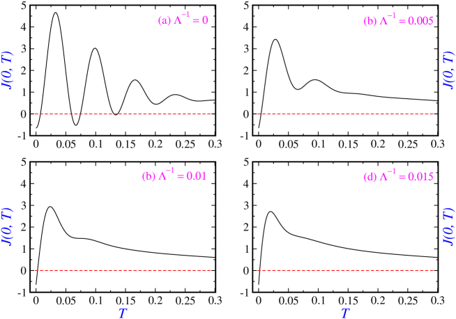
Figure 2: The probability current density at the origin versus time for different values of $\Lambda^{-1}$ for an initial state given by the superposition of two Gaussian wave packets, Eq. (42) (see text for the parameters used).

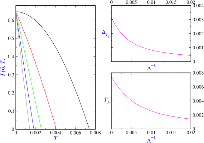
Figure 3: Negative part of the probability current density at the origin (left panel) for different values of $\Lambda^{-1}$: $\Lambda^{-1}=0$ (black), $\Lambda^{-1}=0.005$ (red), $\Lambda^{-1}=0.01$ (green), $\Lambda^{-1}=0.015$ (blue) and $\Lambda^{-1}=0.02$ (brown). In the right two panels, the amount of backflow (top) and the first backflow duration (bottom) for the superposition of two Gaussian wave packets (42) as a function of $\Lambda^{-1}$.

3.1 The Milburn and Lindblad equations

A Lindbladian master equation has the form [36]

$$\frac{\partial}{\partial t}\hat{\rho}(t) = -\frac{i}{\hbar}[\hat{H}^{\prime},\hat{\rho}(t)]-\frac{1}{2}\sum_{\alpha}\kappa_{\alpha}[\hat{L}_{\alpha},[\hat{L}_{\alpha},\hat{\rho}(t)]],$$ (47)

$\hat{H}^{\prime}$ being the the renormalized (Lamb-shifted) Hamiltonian of the system, $\hat{L}_{\alpha}$ the so-called Lindblad operators and a family of parameters $\kappa_{\alpha}\geq 0$. For free particles, the subject of our study, this master equation with just one Lindblad operator recasts

$$\frac{\partial}{\partial t}\hat{\rho}(t) = -\frac{i}{\hbar}[\frac{\hat{p}^{2}}{2m},\hat{\rho}(t)]-\frac{1}{2}\kappa[\hat{L},[\hat{L},\hat{\rho}(t)]].$$ (48)

Comparison of the Milburn equation with the power-expanded in inverse of the time step, $\lambda^{-1}$,

$$\frac{\partial}{\partial t}\hat{\rho}(t) = -\frac{i}{\hbar}[\frac{\hat{p}^{2}}{2m},\hat{\rho}(t)]-\frac{1}{2\hbar^{2}\lambda}[\frac{\hat{p}^{2}}{2m},[\frac{\hat{p}^{2}}{2m},\hat{\rho}(t)]]$$ (49)

with the master equation (48) reveals that this equation, in its expanded form, is just a Lindbladian master equation with only a Lindblad operator proportional to $\hat{p}^{2}$. Because of this similarity, one motivates to consider backflow when the Lindblad operator is a different function of only the momentum. To this end, one must first make sure that the contribution of negative momenta to the state remains zero along time. Taking $\hat{L}=f(\hat{p})$, $f$ being an arbitrary well-defined function, from Eq. (48) in the momentum representation we have that

$$\frac{\partial}{\partial t}\rho(p,p^{\prime},t) = \left\{-\frac{i}{\hbar}\frac{p^{2}-p^{\prime 2}}{2m}-\frac{1}{2}\kappa(f(p)-f(p^{\prime}))^{2}\right\}\rho(p,p^{\prime},t)$$ (50)

whose solution reads as

$$\rho(p,p^{\prime},t) = \exp\left[\left(-\frac{i}{\hbar}\frac{p^{2}-p^{\prime 2}}{2m}-\frac{1}{2}\kappa(f(p)-f(p^{\prime}))^{2}\right)t\right]\rho(p,p^{\prime},0).$$ (51)

This equation confirms that the probability density $\rho(p,p,t)$ is independent on time. Thus, if the contribution of negative momenta to the distribution is initially zero it will be so forever. By considering the special simple form $\hat{L}=\hat{p}$, Eq. (48) is expressed as

$$\frac{\partial}{\partial t}\varrho(x,x^{\prime},t) = \left[\frac{i\hbar}{2m}\left(\frac{\partial^{2}}{\partial x^{2}}-\frac{\partial^{2}}{\partial x^{\prime 2}}\right)+\frac{1}{2}\kappa\hbar^{2}\left(\frac{\partial}{\partial x}+\frac{\partial}{\partial x^{\prime}}\right)^{2}\right]\varrho(x,x^{\prime},t)$$ (52)

in the coordinate representation. Such a choice of the Lindblad operator has already been used to study the effect of dephasing in the context of neutron Compton scattering [37]. In terms of the coordinates $(R,r)$, Eq. (52) takes the form (6) with the probability current density matrix

$$j(R,r,t) = \left(\frac{\hbar}{im}\frac{\partial}{\partial r}-\frac{1}{2}\kappa\hbar^{2}\frac{\partial}{\partial R}\right)\varrho(R,r,t).$$ (53)

Expressing $\varrho(x,x^{\prime},t)$ in terms of $\rho(p,p^{\prime},t)$ and using Eq. (53), then one obtains

$$j(0,0) = \frac{1}{4m\pi\hbar}\int_{-\infty}^{\infty}dp\int_{-\infty}^{\infty}dp^{\prime}(p+p^{\prime}-im\hbar\kappa)\rho(p,p^{\prime},0)$$ (54)

for the probability current density at the origin.

We have avoided the more standard decoherence mechanism in which the Lindblad operator is proportional to the position $\hat{x}$ on the grounds that this is incompatible with keeping positive momentum. However, this deserves an in-depth investigation. Taking $\hat{L}=\hat{x}$, Eq. (48) recasts

$$\frac{\partial}{\partial t}\varrho(x,x^{\prime},t) = \left[\frac{i\hbar}{2m}\left(\frac{\partial^{2}}{\partial x^{2}}-\frac{\partial^{2}}{\partial x^{\prime 2}}\right)-\frac{1}{2}\kappa(x-x^{\prime})^{2}\right]\varrho(x,x^{\prime},t)$$ (55)

in the coordinate representation which is the equation of motion for environmental scattering [36]. On the other hand, the Caldeira-Leggett (CL) master equation in the high temperature limit reads as

$$\frac{\partial}{\partial t}\varrho(x,x^{\prime},t) = \left[\frac{i\hbar}{2m}\left(\frac{\partial^{2}}{\partial x^{2}}-\frac{\partial^{2}}{\partial x^{\prime 2}}\right)-\gamma(x-x^{\prime})\left(\frac{\partial}{\partial x}-\frac{\partial}{\partial x^{\prime}}\right)-\frac{D}{\hbar^{2}}(x-x^{\prime})^{2}\right]\varrho(x,x^{\prime},t)$$

where $\gamma$ is the relaxation rate or damping constant and $D=2m\gamma k_{B}T_{e}$ plays the role of the diffusion coefficient ($k_{B}$ is the Boltzmann constant and $T_{e}$ is the temperature of the environment). Comparison with Eq. (55) shows that the CL equation (3.1) is a Lindbladian one only in the negligible dissipation limit where the second term can be ignored. Let us consider now the evolution of a single Gaussian under Eq. (55) where the contribution of negative momenta is addressed by computing the probability of obtaining negative momenta in a measurement. The evolution of the Gaussian wavepacket

$$\psi_{0}(x) = \frac{1}{(2\pi\sigma_{0}^{2})^{1/4}}\exp\left[-\frac{x^{2}}{4\sigma_{0}^{2}}+i\frac{p_{0}}{\hbar}x\right]$$ (57)

under the Lindbladian master equation (55) yields [38]

$$\varrho(R,r,t) = \frac{1}{\sqrt{2\pi a_{2}(t)}}\exp\left[a_{0}(r,t)-\frac{(R-a_{1}(r,t))^{2}}{4a_{2}(t)}\right],$$ (58)

where

$$a_{0}(r,t) = -\left(\frac{1}{8\sigma_{0}^{2}}+\frac{\kappa}{2}t\right)r^{2}+i\frac{p_{0}}{\hbar}r\equiv-a_{02}(t)~{}r^{2}+i~{}a_{01}~{}r,$$ (59)

$$a_{1}(r,t) = \frac{p_{0}}{m}t+i\hbar\left(\frac{1}{4m\sigma_{0}^{2}}t+\frac{\kappa}{2m}t^{2}\right)r\equiv a_{10}(t)+i~{}a_{11}(t)~{}r,$$ (60)

$$a_{2}(t) = \frac{\sigma_{0}^{2}}{2}\left(1+\frac{\hbar^{2}}{4m^{2}\sigma_{0}^{4}}t^{2}+\frac{\hbar^{2}\kappa}{3m^{2}\sigma_{0}^{2}}t^{3}\right).$$ (61)

The argument of the exponential function in Eq. (58) can be written as

$$-\frac{(R-a_{10}(t))^{2}}{4a_{2}(t)}+i\frac{Ra_{11}(t)-a_{10}(t)a_{11}(t)+2a_{01}a_{2}(t)}{2a_{2}(t)}r-\left(a_{02}(t)-\frac{a_{11}(t)^{2}}{4a_{2}(t)}\right)r^{2}$$ (62)

in powers of $r$ from which one obtains widths in the diagonal, $x=x^{\prime}$, and off-diagonal, $x=-x^{\prime}$, directions respectively as

$$\sigma_{t} = \sqrt{2a_{2}(t)}=\sigma_{0}\sqrt{1+\frac{\hbar^{2}}{4m^{2}\sigma_{0}^{4}}t^{2}+\frac{\hbar^{2}\kappa}{3m^{2}\sigma_{0}^{2}}t^{3}},$$ (63)

$$\ell(t) = \left\{8\left(a_{02}(t)-\frac{a_{11}(t)^{2}}{4a_{2}(t)}\right)\right\}^{-1/2},$$ (64)

where $\sigma_{t}$ is width of the probability density $\varrho(R=x,r=0,t)$ and the so-called coherence length $\ell(t)$ measures the characteristic distance over which the system can exhibit spatial interference effects [36]. The short time behaviour of the coherence length is given by

$$\ell(t) \approx \sigma_{0}\left[1-2\sigma_{0}^{2}\kappa~{}t+\left(\frac{\hbar^{2}}{8m^{2}\sigma_{0}^{4}}+6\sigma_{0}^{4}\kappa^{2}\right)t^{2}\right].$$ (65)

From this, one can extract the decoherence time-scale to be

$$\tau_{\mbox{decoh}}\sim\frac{1}{2\sigma_{0}^{2}\kappa}.$$ (66)

Schlosshauer [36] takes this time-scale as the localization time-scale while it should be instead $\sqrt{m/(\hbar\kappa)}$ (see for instance Ref. [39].) There is another way to extract the decoherence time. The time evolution of the density matrix $\varrho(x,x^{\prime},t)$ under only the non-unitary term $-\frac{1}{2}\kappa(x-x^{\prime})^{2}$ in Eq. (55) yields

$$\varrho(x,x^{\prime},t) = \varrho(x,x^{\prime},0)\exp\left[-\frac{1}{2}\kappa(x-x^{\prime})^{2}~{}t\right].$$ (67)

This shows that the suppression of off-diagonal terms (coherences) increases exponentially with time and with the squared separation $(\Delta x)^{2}=(x-x^{\prime})^{2}$. From Eq. (67), one defines a decoherence time-scale as

$$\tau_{\Delta x}=\frac{2}{\kappa(\Delta x)^{2}}.$$ (68)

For an initial superposition of localized states a distance $b$ apart, the decoherence time-scale has been obtained to be $4/(\kappa b^{2})$.

Now the evolution in the momentum space is carried out by means of the Fourier transform of Eq. (57) which gives

$$\phi_{0}(x) = \left(\frac{2\sigma_{0}^{2}}{\pi\hbar^{2}}\right)^{1/4}\exp\left[-\frac{\sigma_{0}^{2}}{\hbar^{2}}(p-p_{0})^{2}\right]$$ (69)

and leads to [35]

$$\rho(p,p,t) = \frac{1}{\sqrt{2\pi}w_{t}}\exp\left[-\frac{(p-p_{0})^{2}}{2w_{t}^{2}}\right],\qquad w_{t}=\frac{\hbar}{2\sigma_{0}}\sqrt{1+4\kappa\sigma_{0}^{2}t},$$ (70)

for the probability density from which one obtains

$$\mbox{Pr}(p<0,t) = \frac{1}{2}\mbox{erfc}\left[\frac{p_{0}}{\sqrt{2}w_{t}}\right],$$ (71)

for the probability of obtaining a negative value for momentum. The width $w_{t}$ increases with time. Thus, the argument of the complementary error function in Eq. (71) is a decreasing function of time revealing that the probability $\mbox{Pr}(p<0,t)$ is an increasing function of time. In this way, we have that $\tau_{a}\sim 1/(4\kappa\sigma_{0}^{2})$ is the time where negative momenta start appearing, taking $p_{0}\sigma_{0}$ at the same order of $\hbar$. These negative momenta affect the probability of finding the particle in the negative half-space

$$\mbox{Pr}(x<0,t) = \int_{-\infty}^{0}dx^{\prime}\varrho(x,x,t)=\frac{1}{2}\mbox{erfc}\left[\frac{(p_{0}/m)t}{\sqrt{2}\sigma_{t}}\right].$$ (72)

The argument of this complementary error function becomes a decreasing function of time for times greater than $\tau_{s}=(6m^{2}\sigma_{0}^{2}/(\hbar^{2}\kappa))^{1/3}$. This is the time where the effect of negative momenta is reflected in the position. In figure 4, both the probability of obtaining a negative value in a measurement of momentum (left panel) and the probability of finding the particle in the negative half-space (right panel) are plotted. As this figure shows, $\tau_{s}$ is at least one order of magnitude greater than $\tau_{a}$.

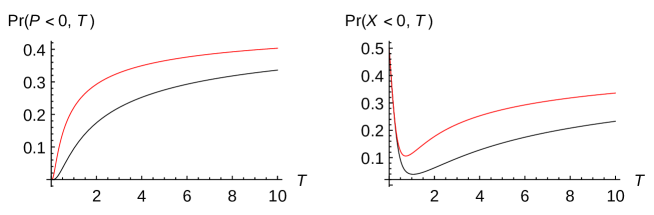
Figure 4: $\mbox{Pr}(P<0,T)=\mbox{erfc}[\sqrt{2}P_{0}/\sqrt{1+4\bar{\kappa}T}]/2$ (right panel) and $\mbox{Pr}(X<0,T)=\mbox{erfc}[P_{0}T/(\sqrt{2}\sqrt{1+T^{2}/4+\bar{\kappa}T^{3}/3})]/2$ (left panel) for $P_{0}=3$ for $\bar{\kappa}=5$ (black) and $\bar{\kappa}=15$ (red). For units of length, time and $\kappa$ we have used respectively $\sigma_{0}$, $\sigma_{0}^{2}m/\hbar$ and $\hbar/(m\sigma_{0}^{4})$. Note that for $P_{0}=3$ the probability for obtaining negative values in a measurement of momentum given by Eq. (71) is initially of the order of $10^{-10}$.

4 Backflow in the framework of the quantum to classical transition wave equation

4.1 Preliminaries

The so-called classical non-linear Schrödinger equation is written as [40]

$$i\hbar\frac{\partial\psi_{\mbox{cl}}(x,t)}{\partial t} = \left[-\frac{\hbar^{2}}{2m}\frac{\partial^{2}}{\partial x^{2}}+V(x)+\frac{\hbar^{2}}{2m}\frac{1}{\mid\psi_{\mbox{cl}}(x,t)\mid}\frac{\partial^{2}\mid\psi_{\mbox{cl}}(x,t)\mid}{\partial x^{2}}\right]\psi_{\mbox{cl}}(x,t),$$

which can be obtained from the quantum to classical transition wave equation

$$i\hbar\frac{\partial}{\partial t}\psi_{\epsilon}(x,t) = \left[-\frac{\hbar^{2}}{2m}\frac{\partial^{2}}{\partial x^{2}}+V(x)+(1-\epsilon)\frac{\hbar^{2}}{2m\mid\psi_{\epsilon}(x,t)\mid}\frac{\partial^{2}\mid\psi_{\epsilon}(x,t)\mid}{\partial x^{2}}\right]\psi_{\epsilon}(x,t).$$

This non-linear transition wave equation was proposed for a continuous transition from the quantum to the classical regime [27] and has been proven to be equivalent to the so-called linear scaled wave equation [27]

$$i\tilde{\hbar}\frac{\partial}{\partial t}\tilde{\psi}(x,t) = \left[-\frac{\tilde{\hbar}^{2}}{2m}\frac{\partial^{2}}{\partial x^{2}}+V(x)\right]\tilde{\psi}(x,t),$$ (75)

where

$$\tilde{\hbar} = \hbar~{}\sqrt{\epsilon}$$ (76)

is the scaled Planck constant with $\epsilon$ being a continuous parameter going from unity (quantum regime) to zero (classical regime). The scaled wave function $\tilde{\psi}(x,t)$ is written in terms of the transition wave function $\psi_{\epsilon}(x,t)$ as

$$\tilde{\psi}(x,t) = \psi_{\epsilon}(x,t)\exp\left[\frac{i}{\hbar}\left(\frac{1}{\sqrt{\epsilon}}-1\right)S_{\epsilon}(x,t)\right],$$ (77)

with $S_{\epsilon}(x,t)$ being the phase of the transition wave function. For an ensemble of classical particles, positions are distributed according to Born rule $\mid\psi_{\mbox{cl}}\mid^{2}$ while momenta are uniquely determined via $p=\partial S_{cl}/\partial x$; $S_{cl}$ being the phase of the classical wave function. In this context, the $\epsilon$ parameter is going to play a similar role as $\lambda$ in the Milburn approach. The intrinsic decoherence process is ruled now by $\epsilon$ when going from one to zero.

From the linear scaled Schrödinger equation (75), one obtains the continuity equation

$$\frac{\partial\tilde{\rho}}{\partial t}+\frac{\partial\tilde{j}}{\partial x} = 0,$$ (78)

where the scaled probability density and probability current density are

$$\tilde{\rho}(x,t)=|\tilde{\psi}(x,t)|^{2},$$ (79)

$$\tilde{j}(x,t)=\frac{\tilde{\hbar}}{m}\mbox{Im}\left\{\tilde{\psi}^{*}(x,t)\frac{\partial}{\partial x}\tilde{\psi}(x,t)\right\},$$ (80)

respectively. Thus, from Eq. (78), one again finds, after integration over the negative part of the space and assuming $\tilde{j}(-\infty,t)=0$, that

$$\frac{d}{dt}\tilde{P}(t) = -\tilde{j}(0,t),$$ (81)

where $\tilde{P}(t)$ is the scaled probability of finding the particle in the negative half-space $x<0$. If $\tilde{j}(0,0)$ is negative, then, by continuity in time, $\tilde{j}(0,t)$ will be negative over some time interval, say $[0,\tilde{t}_{b})$ [2]. Similarly to previous sections, the right-to-left transmitted probability in this time interval is given by

$$\tilde{\Delta}_{\tilde{t}_{b}} = \tilde{P}(\tilde{t}_{b})-\tilde{P}(0)=-\int_{0}^{\tilde{t}_{b}}dt~{}\tilde{j}(0,t)=\int_{0}^{\tilde{t}_{b}}dt~{}\tilde{j}_{{}_{-}}(0,t),$$ (82)

by introducing again

$$\tilde{j}_{{}_{-}}(0,t) = \frac{|\tilde{j}(0,t)|-\tilde{j}(0,t)}{2}$$ (83)

in terms of the corresponding scaled function. If the contribution of positive momenta to the wavefunction at all times is zero, then one speaks of backflow and the interval $[0,\tilde{t}_{b})$ is the backflow interval.

As before, we are going to work on dimensionless variables. By using the same definitions as given by Eqs. (29), (30), and (31), and adding a few more for the scaled functions

$$\tilde{\Psi}(X,T) = \sqrt{\mu}~{}\tilde{\psi}(x,t),$$ (84)

$$\tilde{\Phi}(P,T) = \sqrt{\frac{\hbar}{\mu}}~{}\tilde{\phi}(p,t),$$ (85)

$$\tilde{J}(X,T) = \nu~{}\tilde{j}(x,t),$$ (86)

$$\tilde{G}(X,X^{\prime};T) = \mu~{}\tilde{g}(x,x^{\prime};t),$$ (87)

the coordinate-space scaled wave function

$$\tilde{\psi}(x,t) = \int_{-\infty}^{\infty}dx^{\prime}~{}\tilde{g}(x,x^{\prime};t)~{}\tilde{\psi}(x^{\prime},0)$$ (88)

is expressed now as

$$\tilde{\Psi}(X,T) = \int_{-\infty}^{\infty}dX^{\prime}~{}\tilde{G}(X,X^{\prime};T)~{}\tilde{\Psi}(X^{\prime},0)$$ (89)

for the dimensionless wave function. For free particles, the corresponding wave function can also be obtained from the momentum space wave function as follows

$$\tilde{\psi}(x,t) = \frac{1}{\sqrt{2\pi\tilde{\hbar}}}\int dp~{}e^{i(px-p^{2}t/2m)/\tilde{\hbar}}\tilde{\phi}(p),$$ (90)

or

$$\tilde{\Psi}(X,T) = \frac{1}{\epsilon^{1/4}}\frac{1}{\sqrt{2\pi}}\int dP~{}e^{i(PX-P^{2}T/2)/\sqrt{\epsilon}}~{}\tilde{\Phi}(P).$$ (91)

4.2 Backflow as an eigenvalue problem

Bracken and Melloy [2] showed that the highest probability which can flow back from positive to negatives values of the coordinate is around 0.04. The maximum amount of backflow probability occurring in general over any finite time interval is independent on the time interval, mass of the particle and Planck constant. A new dimensionless quantum number was then proposed. Recently, Bracken [33], in an effort to partially solving the classical limit of backflow, has generalized the study to wave functions whose momentum contributions is within an arbitrary interval instead of the original one $[0,\infty)$. Here, in this subsection, we are going to carry out the same study but in the context of the scaled Schrödinger equation by considering the momentum contribution in the interval $[p_{0},\infty)$; $p_{0}$ being an arbitrary non-negative number. Using Eqs. (90) and (82), one obtains

$$\tilde{\Delta}_{\tilde{t}_{b}} = -\frac{1}{\pi}\int_{p_{0}}^{\infty}\int_{p_{0}}^{\infty}dp~{}dq~{}\tilde{\phi}^{*}(p)\frac{\sin[(p^{2}-q^{2})\tilde{t}_{b}/4m\tilde{\hbar}]}{p-q}~{}e^{i(p^{2}-q^{2})\tilde{t}_{b}/4m\tilde{\hbar}}\tilde{\phi}(q).$$

Now to find the optimum value of the right-to-left transported probability $\tilde{\Delta}_{\tilde{t}_{b}}$, one should optimize the integral of Eq. (4.2) subject to the normalization condition

$$\int_{p_{0}}^{\infty}dp|\tilde{\phi}(p)|^{2} = 1,$$ (93)

by using the method of Lagrange multipliers. After some straightforward algebra, one sees that the only Lagrange multiplier equals $\tilde{\Delta}_{\tilde{t}_{b}}$ and appears as the eigenvalue of the integral equation

$$-\frac{1}{\pi}\int_{p_{0}}^{\infty}\frac{\sin[(p^{2}-q^{2})\tilde{t}_{b}/4m\tilde{\hbar}]}{p-q}\tilde{\phi}(q) = \tilde{\Delta}(p_{0})~{}\tilde{\phi}(p),$$ (94)

where, for simplicity, we have dropped the sub-index $\tilde{t}_{b}$ and for clarity we have introduced the right-to-left transported probability as a function of $p_{0}$. By setting

$$p=2\sqrt{\frac{m\tilde{\hbar}}{\tilde{t}_{b}}}~{}u$$ (95)

$$q=2\sqrt{\frac{m\tilde{\hbar}}{\tilde{t}_{b}}}~{}v$$ (96)

$$\phi(p)=e^{iu^{2}}\varphi(u)$$ (97)

$$\phi(q)=e^{iv^{2}}\varphi(v)$$ (98)

the eigenvalue equation (94) can be written as

$$-\frac{1}{\pi}\int_{\tilde{u}_{0}}^{\infty}dv~{}\frac{\sin(u^{2}-v^{2})}{u-v}\varphi(v) = \tilde{\Delta}(\tilde{u}_{0})\varphi(u).$$ (99)

where $\tilde{u}_{0}=p_{0}\sqrt{\tilde{t}_{b}/4m\hbar\sqrt{\epsilon}}$.

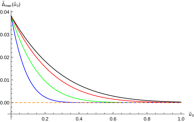
Figure 5: Maximum eigenvalue $\tilde{\Delta}_{\max}$ versus $\tilde{u}_{0}$ for different dynamical regimes: quantum (black), non-classical with $\epsilon=0.5$ (red), $\epsilon=0.1$ (green) and $\epsilon=0.01$ (blue) and classical (dashed orange).

In figure 5 we have plotted the maximum backflow probability $\tilde{\Delta}_{\max}(\tilde{u}_{0})$ versus $\tilde{u}_{0}$ for different dynamical regimes keeping the same backflow interval $\tilde{t}_{b}$. As clearly seen, for all the dynamical regimes, $\tilde{\Delta}_{\max}(\tilde{u}_{0})$ decreases with $\tilde{u}_{0}$. Furthermore, in the classical limit $\epsilon\rightarrow 0$, this probability approaches zero irrespective of $\tilde{u}_{0}$.

4.3 Bracken and Melloy classical example

Let us now consider a free particle which is described initially by the normalized wave function [2]

$$\tilde{\phi}(p) = \frac{18}{\sqrt{35~{}\tilde{\hbar}k}}\frac{p}{\tilde{\hbar}k}\left(e^{-p/\tilde{\hbar}k}-\frac{1}{6}e^{-p/2\tilde{\hbar}k}\right)\Theta(p),$$ (100)

in the momentum space where $k$ is a positive wave number. Expressing space and time coordinates from Eqs. (40) and (41) and using Eqs. (85), (86) and (91), one has that

$$\tilde{\Phi}(P)=\frac{1}{\epsilon^{3/4}}\frac{18}{\sqrt{35}}P\left(e^{-P/\sqrt{\epsilon}}-\frac{1}{6}e^{-P/(2\sqrt{\epsilon})}\right)\Theta(P)$$ (101)

$$\tilde{\Psi}(X,T)=\frac{1}{\epsilon^{1/4}}\frac{1}{\sqrt{2\pi}}\int dP~{}e^{i(PX-P^{2}T/2)/\sqrt{\epsilon}}~{}\tilde{\Phi}(P)$$ (102)

$$\tilde{J}(X,T)=\sqrt{\epsilon}~{}\mbox{Im}\left\{\tilde{\Psi}^{*}(X,T)\frac{\partial}{\partial X}\tilde{\Psi}(X,T)\right\}$$ (103)

and

$$\tilde{J}(0,0) = -\sqrt{\epsilon}\frac{36}{35\pi}$$ (104)

which is explicitly negative for all non-classical regimes and revealing the occurrence of backflow for all regimes except the classical one. This effect will not be certainly observed for the classical regime $\epsilon=0$ since $J_{cl}(0,0)=0$.

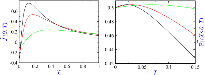
Figure 6: The probability current density given by Eq. (103) (left panel) and the probability of remaining in the negative half-space (right panel) for different dynamical regimes: quantum (black) and non-classical (red and green with $\epsilon=0.5$ and $\epsilon=0.1$, respectively).

As figure 6 displays, the backflow interval increases while the negativity of the probability current density decreases in the quantum-to-classical transition. As should be expected, computations show that Eq. (82) is almost the same for all non-classical regimes; $\tilde{\Delta}\simeq 0.004251$.

Several years ago, Halliwell et al. [41] considered quantum backflow states from eigenstates of the so-called regularized current operator. They used a general function of momenta subject to special conditions, leading to a surprisingly large backflow of about 41 $\%$ of the lower bound on flux derived by Bracken and Melloy.

4.4 A superposition of two Gaussian wave packets

As an another illustration of backflow, we have solved the scaled Schrödinger equation (75) for free particles by considering an initial wave function as a superposition of two co-centred Gaussian wave packets with the same width but different kick momenta

$$\tilde{\psi}_{0}(x) = \tilde{N}(\tilde{\psi}_{a}(x,0)+\alpha e^{i\theta}\tilde{\psi}_{b}(x,0))$$ (105)

$$= \tilde{N}\frac{1}{(2\pi\sigma_{0}^{2})^{1/4}}(e^{ip_{0a}x/\tilde{\hbar}}+\alpha e^{i\theta}e^{ip_{0b}x/\tilde{\hbar}})~{}e^{-x^{2}/4\sigma_{0}^{2}},$$

with

$$\tilde{N} = \left(1+\alpha^{2}+2\alpha e^{-\sigma_{0}^{2}(p_{0a}-p_{0b})^{2}/2\tilde{\hbar}^{2}}\cos\theta\right)^{-1/2},$$ (106)

and $\alpha$ and $\theta$ being two arbitrary real numbers. Here space and time coordinates are expressed in terms of

$$\mu=\sigma_{0},$$ (107)

$$\nu=\frac{\mu^{2}m}{\hbar}=\frac{m\sigma_{0}^{2}}{\hbar}.$$ (108)

The solution of the scaled Schrödinger equation (75) yields [20]

$$|\tilde{\Psi}(X,T)|^{2} = \tilde{N}^{2}\frac{1}{\sqrt{2\pi}\tilde{\Sigma}_{T}}\bigg{\{}\exp\left[-\frac{(X-P_{0a}T)^{2}}{2\tilde{\Sigma}_{T}^{2}}\right]+\alpha\exp\left[\tilde{D}_{1}-\frac{(X-\tilde{D}_{2}(T))^{2}}{2\tilde{\Sigma}_{T}^{2}}\right]$$ (109)

$$+ \alpha\exp\left[\tilde{D}_{1}^{*}-\frac{(X-\tilde{D}_{2}^{*}(t))^{2}}{2\tilde{\Sigma}_{T}^{2}}\right]+\alpha^{2}\exp\left[-\frac{(X-P_{0b}T)^{2}}{2\tilde{\Sigma}_{T}^{2}}\right]\bigg{\}}$$

for the probability density, where

$$\tilde{\Sigma}_{T} = \sqrt{1+\epsilon~{}T^{2}/4}$$ (110)

is the width of each wave packet and

$$\tilde{D}_{1}=-i\theta-\frac{(P_{0a}-P_{0b})^{2}}{2\epsilon}$$ (111)

$$\tilde{D}_{2}(T)=\frac{(P_{0a}+P_{0b})T}{2}+i\frac{P_{0a}-P_{0b}}{\sqrt{\epsilon}}$$ (112)

$$\tilde{N}=\left(1+\alpha^{2}+2\alpha e^{-(P_{0a}-P_{0b})^{2}/2\epsilon}\cos\theta\right)^{-1/2}.$$ (113)

The momentum space wave function can be obtained as follows

$$\tilde{\phi}(p,t) = \langle p|\tilde{\psi}(t)\rangle=\langle p|e^{-i\hat{H}t/\tilde{\hbar}}|\tilde{\psi}_{0}\rangle=e^{-ip^{2}t/2m\tilde{\hbar}}\tilde{\phi}_{0}(p),$$ (114)

where $\tilde{\phi}_{0}(p)$ is the Fourier transform of $\tilde{\psi}_{0}(x)$. With dimensionless variables, one has that

$$\tilde{\Phi}_{0}(P) = \tilde{N}\frac{1}{(2\pi)^{1/4}}\frac{\sqrt{2}}{\epsilon^{1/4}}\left\{\exp\left[-\frac{(P-P_{0a})^{2}}{\epsilon}\right]+\alpha e^{i\theta}\exp\left[-\frac{(P-P_{0b})^{2}}{\epsilon}\right]\right\}.$$

Thus, the probability for obtaining a negative value in a measurement of momentum is time-independent and given by

$$\tilde{\mbox{Pr}}(p<0) = \int_{-\infty}^{0}dp~{}|\tilde{\phi}(p,t)|^{2}=\int_{-\infty}^{0}dP~{}|\tilde{\Phi}(P,T)|^{2}$$ (116)

$$= \frac{\tilde{N}^{2}}{2}\bigg{\{}\mbox{erfc}\left[\frac{\sqrt{2}P_{0a}}{\sqrt{\epsilon}}\right]+\alpha^{2}\mbox{erfc}\left[\frac{\sqrt{2}P_{0b}}{\sqrt{\epsilon}}\right]$$

$$+ 2\alpha~{}e^{-(P_{0a}-P_{0b})^{2}/2\epsilon}\cos\theta~{}\mbox{erfc}\left[\frac{(P_{0a}+P_{0b})}{\sqrt{2\epsilon}}\right]\bigg{\}}.$$

For backflow, one should make sure that the contribution of negative momenta to the wavefunction is zero. To this end, the parameters of the problem should be chosen in a way that $\tilde{\mbox{Pr}}(p<0)$ is negligible. Two points are in order: (i) the width of each Gaussian wave packets in the momentum space is $\tilde{\sigma}_{p}=\tilde{\hbar}/2\sigma_{0}$ which becomes zero in the classical regime $\epsilon=0$. (i)) Eq. (116) shows that $\tilde{\mbox{Pr}}(p<0)$ is zero in the classical regime $\epsilon=0$ apart from the values of the involved parameters.

From the probability density Eq. (109), one obtains

$$\tilde{\mbox{Pr}}(X<0,T) = \frac{1}{2}\tilde{N}^{2}\bigg{\{}\mbox{erfc}\left[P_{0a}T/\sqrt{2}\tilde{\Sigma}_{T}\right]+\alpha^{2}\mbox{erfc}\left[P_{0b}T/\sqrt{2}\tilde{\Sigma}_{T}\right]$$ (117)

$$+ 2\alpha e^{-(P_{0a}-P_{0b})^{2}/2\epsilon}\bigg{(}\cos\theta~{}\mbox{Re}\left\{\mbox{erfc}\left[\tilde{D}_{2}(T)/(\sqrt{2}~{}\tilde{\Sigma}_{T})\right]\right\}$$

$$+ \sin\theta~{}\mbox{Im}\left\{\mbox{erfc}\left[\tilde{D}_{2}(T)/(\sqrt{2}~{}\tilde{\Sigma}_{T})\right]\right\}\bigg{)}\bigg{\}}$$

for the probability of remaining in the negative half-space $x<0$. Eq. (117) shows that, in the classical regime, the contribution of interference terms becomes zero and the first two terms are decreasing functions of time. Thus, backflow is not observed in the classical realm while it is so in the remaining non-classical regimes.

In figure 7, we have plotted the probability in the negative half-space in terms of time for different regimes. For numerical computations, we have chosen $P_{0a}=14$, $P_{0b}=3$, $\alpha=1.9$ and $\theta=\pi$. For these values, $\tilde{Pr}(p<0)$ is of the order of $10^{-10}$ for the quantum regime and even lesser for the remaining regimes. The probability of backflow is thus observed for all non-classical regimes $\epsilon\neq 0$ except the classical one.

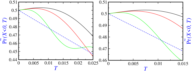
Figure 7: Probability of remaining in the negative half-space $x<0$ given by Eq. (117) for different dynamical regimes: quantum (black), non-classical (red and green with $\epsilon=0.5$ and $\epsilon=0.1$, respectively) and classical (blue). The right panel is a close-up of the left one around the origin.

5 Intrinsic decoherence in dissipative backflow

In the Caldirola-Kanai framework for dissipative dynamics coming from an effective Hamiltonian, the time-dependent Schrödinger equation reads as

$$i\hbar\frac{\partial}{\partial t}\psi(x,t) = \bigg{[}-e^{-2\gamma t}\frac{\hbar^{2}}{2m}\frac{\partial^{2}}{\partial x^{2}}+e^{2\gamma t}V(x)\bigg{]}\psi(x,t),$$ (118)

where $\gamma$ is the dissipation rate or friction coefficient. Then, the scaled transition equation in this context is obtained as [28, 29]

$$i\tilde{\hbar}\frac{\partial}{\partial t}\tilde{\psi}(x,t) = \bigg{[}-e^{-2\gamma t}\frac{\tilde{\hbar}^{2}}{2m}\frac{\partial^{2}}{\partial x^{2}}+e^{2\gamma t}V(x)\bigg{]}\tilde{\psi}(x,t).$$ (119)

In this framework, the continuity equation again has the form (78) but with

$$\tilde{j}(x,t) = \frac{\tilde{\hbar}}{m}\mbox{Im}\left\{\tilde{\psi}^{*}\frac{\partial\tilde{\psi}}{\partial x}\right\}e^{-2\gamma t},$$ (120)

as the probability current density. The propagator of the free particle in the context of dissipative transition equation is given by [29]

$$\tilde{g}_{\mbox{free}}(x,x^{\prime};t) = \sqrt{\frac{m}{2\pi i\tilde{\hbar}\tau(t)}}\exp\left[\frac{im}{2\tilde{\hbar}\tau(t)}(x-x^{\prime})^{2}\right],$$ (121)

where

$$\tau(t) = \frac{1-e^{-2\gamma t}}{2\gamma}.$$ (122)

By introducing dimensionless time and relaxation coefficient according to

$$T=\frac{t}{\nu}$$ (123)

$$\Gamma=\nu~{}\gamma,$$ (124)

one obtains

$$\tau(t) = \nu\frac{1-e^{-2\Gamma T}}{2\Gamma}\equiv\nu~{}\uptau(T).$$ (125)

Now, by expressing the space coordinate versus $\mu=\sqrt{\nu\hbar/m}$, one has

$$\tilde{g}_{\mbox{free}}(x,x^{\prime};t) = \frac{1}{\mu}\frac{1}{\epsilon^{1/4}}\frac{1}{\sqrt{2\pi i~{}\uptau(T)}}\exp\left[\frac{i}{2\sqrt{\epsilon}\uptau(T)}(X-X^{\prime})^{2}\right]\equiv\frac{1}{\mu}\tilde{G}_{\mbox{free}}(X,X^{\prime};T)$$

for the propagator and for the time-evolved wave function

$$\tilde{\Psi}(X,T) = \int_{-\infty}^{\infty}dX^{\prime}~{}\tilde{G}_{free}(X,X^{\prime};T)~{}\tilde{\Psi}(X^{\prime},0).$$ (127)

Comparison of Eq. (5) with the corresponding one for the non-dissipative case shows that previous results are valid replacing $T$ by $\uptau(T)$.

For an illustration, in figure 8, the negative part of the probability current density Eq. (83) at the origin versus time for the quantum regime with different values of $\gamma$ (left panel) and for different non-classical regimes with a given value of $\gamma$ (right panel) are shown. The initial wave function is given by Eq. (101). As expected, the amount of backflow increases with damping in the quantum regime. On the contrary, in the quantum to classical transition, the negativity of the probability current density is again reduced.

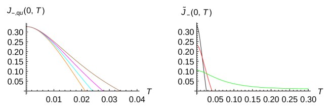
Figure 8: Negative part of the probability current density at the origin for different values of $\Gamma$ in the quantum regime (left panel). In the right panel, the same function is plotted for different non-classical regimes at $\Gamma=8$. The initial wave function is given by Eq. (101). Colour codes in the left panel are: $\Gamma=0$ (orange), $\Gamma=5$ (cyan), $\Gamma=10$ (magenta) and $\Gamma=15$ (brown); and in the right panel: $\epsilon=1$ (black), $\epsilon=0.5$ (red) and $\epsilon=0.1$ (green).

6 Conclusions

Along this work we have emphasized the importance of the intrinsic decoherence in backflow. This effect is gradually suppressed as the the corresponding process is developing. The emergence of classical mechanics or classical limit is quite similar irrespective of the theoretical method used, namely: the generalized von Neumann equation proposed by Milburn and the linear scaled wave equation which itself is equivalent to the non-linear transition wave equation. By considering various examples, we have shown that the intrinsic decoherence diminishes both the backflow amount and also its duration. As far as we know, this is the first time backflow has been considered in the most general formulation of quantum mechanics in terms of density matrices instead of wavefunctions and for isolated systems. Our results show that in the quantum-to-classical transition, this effect attenuates and completely disappears in the classical regime. This confirms us that backflow is a non-classical effect occurring in all non-classical dynamical regimes, including quantum mechanics. This should not be confused with the fact that this effect is seen even for classical waves [8]. The important point is that the backflow is an interference phenomenon which itself has a wave nature [11, 12]. Thus, only quantum particles with their dual character can exhibit this wave phenomenon. This situation is quite similar to tunnelling: while the effect is considered genuinely quantum mechanical, its classical optical analogue, frustrated total reflection, exists [34]. Another important point to be stressed is that the linearity of the wave equation is not necessary to see this wave phenomenon. Actually, as also shown here, a nonlinear Schrödinger wave equation reproduces all the features of linear quantum mechanics [27]. Moreover, one of the main messages we want to convey is that the route to the classical limit is not unique i.e., there is not only one way to classicality. Intrinsic decoherence can also have several sources depending on the starting point. Even more, for completeness, a parallel theoretical analysis has been carried out in terms of the Linblad equation. Finally, it is also shown that the appearance of classicality through dissipative dynamics can not be comparable to the previous routes used.

Backflow has already been studied for both distinguishable [20] and indistinguishable particles [21] in the context of the CK approach. In this work, we have carried out the same analysis but within the scaled CK equation [28, 29]. Previously, a study was carried out within the Caldeira-Leggett formalism [20] by including also temperature but then it was argued that the corresponding results did not imply quantum backflow [42] due to the fact that the positive momentum distribution along time was not maintained. With intrinsic decoherence, extension to important aspects such as, for example, its effect on backflow for two-identical-particle systems and the interference pattern for a superposition of two wave packets are interesting. Work in this direction is now in progress.

7 Acknowledgments

SVM acknowledges support from the University of Qom. SMA would like to thank support from Fundación Humanismo y Ciencia. Furthermore, we thank the anonymous reviewers for their careful reading of our manuscript and their many insightful comments and suggestions.

References

- [1] Allcock G R 1969 Ann. Phys. 53 253; ibid 53 286; ibid 53 311
- [2] Bracken A J and Melloy G F 1994 J. Phys. A Math. Gen. 27 2197
- [3] Penz M, Grübl G, Kreidl S and Wagner P 2006 J. Phys. A: Math. Gen. 39 423
- [4] Bracken A J and Melloy G F (1998) Ann. Phys. (Leipzig) 7 726
- [5] Melloy G F and Bracken A J 1998 Found. Phys. 28 505
- [6] Su H-Y and Chen J-L 2018 Mod. Phys. Lett. A 33 1850186
- [7] Ashfaque J, Lynch J and Strange P 2019 Phys. Scr. 94 125107
- [8] Bialynicki-Birula I, Bialynicki-Birula Z and Augustynowicz S 2022 J. Phys. A: Math. Theor. 55 255702
- [9] Yearsley J M and Halliwell J J 2013 J. Phys.: Conference Serie 442 012055
- [10] Grübl G, Kreidl S, Penz M and Ruggenthaler M 2006 AIP Conf. Proc. 844 177
- [11] Goussev A 2019 Phys. Rev. A 99 043626
- [12] Goussev A 2020 Phys. Rev. Research 2 033206
- [13] Miller M, Yuan W C, Dumke R and Paterek T 2021 Quantum 5 379
- [14] Barbier M and Goussev A 2021 Quantum 5 536
- [15] Strange P 2012 Eur. J. Phys. 33 1147
- [16] Paccoia V D, Panella O and Roy P 2020 Phys. Rev. A 102 062218
- [17] Goussev A 2021 Phys. Rev. A 103 022217
- [18] Paccoia V D, Panella O and Roy P 2022 arXiv:2201.12916v1
- [19] Albarelli F, Guaita T and Paris M G A 2016 Int. J. Quant. Inf. 14 1650032
- [20] Mousavi S V and Miret-Artés S 2020 Eur. Phys. J. Plus 135 324
- [21] Mousavi S V and Miret-Artés S 2020 Results in Phys. 33 1850186
- [22] Barbier M 2020 Phys. Rev. A 102 023334
- [23] Eliezer Y, Zacharias T and Bahabad A 2020 Optica 7 72
- [24] Schlosshauer M 2019 Phys. Rep. 831 1
- [25] Stamp P C E 2012 Phil. Trans. R. Soc. A 370 4429
- [26] Milburn G J 1991 Phys. Rev. A 44 5401
- [27] Richardson C D, Schlagheck P, Martin J, Vandewalle N and Bastin T 2014 Phys. Rev. A 89 032118
- [28] Mousavi S V and Miret-Artés S 2018 Ann. Phys. 393 76
- [29] Mousavi S V and Miret-Artés S 2018 J. Phys. Commun. 2 035029
- [30] Schiller R 1962 Phys. Rev. 125 1100
- [31] Mousavi S V and Miret-Artés S 2022 Found. Phys. 52 78
- [32] Yearsley J M , Halliwell J J, Hartshorn R and Whitby A 2012 Phys. Rev. A 86 042116
- [33] Bracken A J 2021 Phys. Scr. 96 045201
- [34] Krane K 2012 Modern Physics, John Wiley and Sons
- [35] Kani Z, Mousavi S V and Miret-Artés S 2021 Entropy 23 1469
- [36] Schlosshauer M 2007, Decoherence and the Quantum-To-Classical Transition, Springer-Verlag Berlin Heidelberg
- [37] Chatzidimitriou-Dreismann C A and Tietje I C 2010 J. Phys.: Conf. Ser. 237 012010
- [38] Mousavi S V and Miret-Artés S 2022 Eur. Phys. J. Plus 137 1
- [39] Halliwell J and Zoupas A 1997 Phys. Rev. D 55(8) 4697
- [40] Rosen N 1964 Am. J. Phy. 32 597
- [41] Halliwell J J, Gillman E, Lennon O, Patel M and Ramirez I 2013 J. Phys. A: Math. Theor. 46 475303
- [42] Mousavi S V and Miret-Artés S 2020 Eur. Phys. J. Plus 135 654