Numerical accuracy and stability of semilinear Klein–Gordon equation in de Sitter spacetime

Abstract

Numerical simulations of the semilinear Klein–Gordon equation in the de Sitter spacetime are performed. We use two structure-preserving discrete forms of the Klein–Gordon equation. The disparity between the two forms is the discretization of the differential term. We show that one of the forms has higher numerical stability and second-order numerical accuracy with respect to the grid, and we explain the reason for the instability of the other form.

1 Introduction

The Klein–Gordon equation is one of the relativistic wave equations. There have been some analytical investigations of this equation (e.g., [1, 2, 3]). However, it is difficult to quantitatively evaluate the solutions analytically; therefore, we carry out numerical simulations to investigate the solutions. In this paper, we adopt the structure-preserving scheme [4] as a discretized scheme to realize high-accuracy and high-stability simulations. Here, the word “accuracy” means the difference between the initial and time-evolved values of constraints. A value is, for example, the total Hamiltonian in the Hamiltonian system. In general, numerical accuracy means the difference between the exact and numerical solutions. However, the exact solution is usually not obtained for the targets in numerical calculations. Thus, the conservation of the constraint is treated as the numerical accuracy of the system in this paper. In addition, the word “stability” means that the numerical solutions have no numerical vibrations. Precisely, the solution with numerical vibrations is less stable than that without such vibrations.

In our previous paper [5], we reported some numerical results of the solution of the Klein–Gordon equation with the structure-preserving scheme. However, we have recently reported in [6] that numerical stability is not sufficient for the quantitative evaluations of the numerical results in [5]. Thus, we propose another structure-preserving discretized form with higher stability and comparable accuracy to the form in [5].

In this paper, we set the physical constants of the speed of light, the constant of gravitation, and Dirac’s constant as units. Indices such as $(i,j,k,\dots)$ run from 1 to 3. We use the Einstein convention of summation of repeated up–down indices.

2 Semilinear Klein–Gordon equation in de Sitter spacetime

The semilinear Klein–Gordon equation in the de Sitter spacetime (e.g., [5]) is given by

$$-\partial_{t}^{2}\phi-nH\partial_{t}\phi+e^{-2Ht}\delta^{ij}(\partial_{i}\partial_{j}\phi)-m^{2}\phi=|\phi|^{p-1}\phi,$$ (1)

where $\phi$ is the dynamical variable, $n$ is the spacial dimension, $m$ is the mass, $p$ is the integer greater than or equal to 2, and $H$ is the Hubble constant. $H>0$ means the expansion of space; conversely, $H<0$ means the contraction of space. $H=0$ means a flat space.

The Hamiltonian of (1) is given by

$$\mathcal{H} =\dfrac{1}{2}e^{-nHt}\psi^{2}+\dfrac{m^{2}}{2}e^{nHt}\phi^{2}+\dfrac{1}{p+1}e^{nHt}|\phi|^{p+1}+\dfrac{1}{2}e^{(n-2)Ht}\delta^{ij}(\partial_{i}\phi)(\partial_{j}\phi).$$ (2)

Then, the evolution equations are

$$\partial_{t}\phi =e^{-nHt}\psi,$$ (3)

$$\partial_{t}\psi =-m^{2}e^{nHt}\phi-e^{nHt}|\phi|^{p-1}\phi+e^{(n-2)Ht}\delta^{ij}(\partial_{j}\partial_{i}\phi).$$ (4)

The total Hamiltonian $H_{C}$ is defined as

$$H_{C}(t):=\int_{\mathbb{R}^{n}}\mathcal{H}(t,x^{i})\,d^{n}x,$$ (5)

and with (3)–(4), the time derivative of (5) is

$$\partial_{t}H_{C} =\dfrac{H}{2}e^{nHt}\int_{\mathbb{R}^{n}}d^{n}x\biggl{(}-ne^{-2nHt}\psi^{2}+nm^{2}\phi^{2}+\dfrac{2n}{p+1}|\phi|^{p+1}+(n-2)\delta^{ij}e^{-2Ht}(\partial_{i}\phi)(\partial_{j}\phi)\biggr{)}$$

$$\quad+\int_{\mathbb{R}^{n}}d^{n}x\partial_{j}\left(c^{2}\delta^{ij}e^{-2Ht}\psi(\partial_{i}\phi)\right).$$ (6)

Note that $H$ is the Hubble constant and $H_{C}$ is the total Hamiltonian. If we set an appropriate boundary condition such as the periodic boundary condition, the last term on the right-hand side of (6) is eliminated. In addition, if $H=0$, $\partial_{t}H_{C}=0$. This means that $H_{C}$ is constant with time if $H=0$. On the other hand, $H_{C}$ is not constant with time if $H\neq 0$. To make a value constant with time, we define a value as

$$\tilde{H}_{C}(t) :=H_{C}(t)-\int^{t}_{0}\partial_{s}H_{C}(s)ds$$

$$=H_{C}(t)-\dfrac{H}{2}\int^{t}_{0}ds\,e^{nHs}\biggl{\{}\int_{\mathbb{R}^{n}}d^{n}x\biggl{(}-ne^{-2nHs}\psi^{2}+nm^{2}\phi^{2}+\dfrac{2n}{p+1}|\phi|^{p+1}+(n-2)e^{-2Hs}\delta^{ij}(\partial_{i}\phi)(\partial_{j}\phi)\biggr{)}\biggr{\}}.$$ (7)

We call this value the modified total Hamiltonian, which is constant with time if $H\neq 0$. We judge whether the simulations are a success or a failure if $H_{C}$ in $H=0$ or $\tilde{H}_{C}$ in $H\neq 0$ is conserved or not in the time evolution.

3 Discretized form of semilinear Klein–Gordon equation in de Sitter spacetime

In this paper, we use two discretized forms. The first form includes the product of the first-order central difference formulae in the evolution equations. The second form includes the product of the first-order forward and backward difference formulae in the equations. We call the first form Form I and the second one Form II. Form I was suggested in [5], and Form II is a new discretized form of the Klein–Gordon equation.

3.1 Form I

The discretized (2), (3), and (4) can be respectively defined as

$$\mathcal{H}^{\mathrm{I}}{}^{(\ell)}_{(\boldsymbol{k})} :=\frac{1}{2}e^{-nHt^{(\ell)}}(\psi^{(\ell)}_{(\boldsymbol{k})})^{2}+\dfrac{m^{2}}{2}e^{nHt^{(\ell)}}(\phi^{(\ell)}_{(\boldsymbol{k})})^{2}+\dfrac{1}{p+1}e^{nHt^{(\ell)}}|\phi^{(\ell)}_{(\boldsymbol{k})}|^{p+1}+\dfrac{1}{2}e^{(n-2)Ht^{(\ell)}}\delta^{ij}(\widehat{\delta}^{\langle 1\rangle}_{i}\phi^{(\ell)}_{(\boldsymbol{k})})(\widehat{\delta}^{\langle 1\rangle}_{j}\phi^{(\ell)}_{(\boldsymbol{k})}),$$

$$\frac{\phi^{(\ell+1)}_{(\boldsymbol{k})}-\phi^{(\ell)}_{(\boldsymbol{k})}}{\Delta t} :=\dfrac{1}{4}(e^{-nHt^{(\ell+1)}}+e^{-nHt^{(\ell)}})(\psi^{(\ell+1)}_{(\boldsymbol{k})}+\psi^{(\ell)}_{(\boldsymbol{k})}),$$ (8)

$$\frac{\psi^{(\ell+1)}_{(\boldsymbol{k})}-\psi^{(\ell)}_{(\boldsymbol{k})}}{\Delta t} :=-\frac{m^{2}}{4}(e^{nHt^{(\ell+1)}}+e^{nHt^{(\ell)}})(\phi^{(\ell+1)}_{(\boldsymbol{k})}+\phi^{(\ell)}_{(\boldsymbol{k})})-\frac{1}{2(p+1)}(e^{nHt^{(\ell+1)}}\!\!+\!e^{nHt^{(\ell)}})\frac{|\phi^{(\ell+1)}_{(\boldsymbol{k})}|^{p+1}-|\phi^{(\ell)}_{(\boldsymbol{k})}|^{p+1}}{\phi^{(\ell+1)}_{(\boldsymbol{k})}-\phi^{(\ell)}_{(\boldsymbol{k})}}$$

$$\quad+\dfrac{e^{(n-2)Ht^{(\ell+1)}}+e^{(n-2)Ht^{(\ell)}}}{4}\delta^{ij}\widehat{\delta}^{\langle 1\rangle}_{i}\widehat{\delta}^{\langle 1\rangle}_{j}(\phi^{(\ell+1)}_{(\boldsymbol{k})}+\phi^{(\ell)}_{(\boldsymbol{k})}),$$ (9)

where ^(ℓ) means the time index, _(k) means the space index, and $\boldsymbol{k}=(k_{1},\dots,k_{n})$. $\widehat{\delta}^{\langle 1\rangle}$ is the first-order central difference operator defined as

$$\widehat{\delta}^{\langle 1\rangle}_{i}u^{(\ell)}_{(\boldsymbol{k})}:=\dfrac{u^{(\ell)}_{(k_{1},\dots,k_{i}+1,\dots,k_{n})}-u^{(\ell)}_{(k_{1},\dots,k_{i}-1,\dots,k_{n})}}{2\Delta x^{i}}.$$

Here, $\Delta x^{i}$ is the $i$-th grid range. If $n=3$, for example, $\Delta x^{1}=\Delta x$, $\Delta x^{2}=\Delta y$, and $\Delta x^{3}=\Delta z$.

The discretized (5) can be defined as

$${H}^{\mathrm{I}}_{C}{}^{(\ell)}:=\sum_{2\leq k_{1}\leq N_{1}+1}\cdots\sum_{2\leq k_{n}\leq N_{n}+1}\mathcal{H}^{\mathrm{I}}{}^{(\ell)}_{(\boldsymbol{k})}\Delta V,$$ (10)

where $\Delta V=\Delta x^{1}\cdots\Delta x^{n}$ and $N_{i}$ is the number of $i$-th grids. The discretized (7) is defined as

$$\tilde{H}^{\mathrm{I}}_{C}{}^{(\ell)} :=H^{\mathrm{I}}_{C}{}^{(\ell)}-\sum_{q=0}^{\ell-1}(H^{\mathrm{I}}_{C}{}^{(q+1)}-H^{\mathrm{I}}_{C}{}^{(q)})\Delta t.$$ (11)

3.2 Form II

The discretized (2), (4), and (3) can be respectively defined as

$$\mathcal{H}^{\mathrm{II}}{}^{(\ell)}_{(\boldsymbol{k})} :=\frac{1}{2}e^{-nHt^{(\ell)}}(\psi^{(\ell)}_{(\boldsymbol{k})})^{2}+\dfrac{m^{2}}{2}e^{nHt^{(\ell)}}(\phi^{(\ell)}_{(\boldsymbol{k})})^{2}+\dfrac{1}{p+1}e^{nHt^{(\ell)}}|\phi^{(\ell)}_{(\boldsymbol{k})}|^{p+1}$$

$$\quad+\dfrac{1}{4}e^{(n-2)Ht^{(\ell)}}\delta^{ij}\biggl{(}(\widehat{\delta}^{+}_{i}\phi^{(\ell)}_{(\boldsymbol{k})})(\widehat{\delta}^{+}_{j}\phi^{(\ell)}_{(\boldsymbol{k})})+(\widehat{\delta}^{-}_{i}\phi^{(\ell)}_{(\boldsymbol{k})})(\widehat{\delta}^{-}_{j}\phi^{(\ell)}_{(\boldsymbol{k})})\biggr{)},$$ (12)

$$\frac{\psi^{(\ell+1)}_{(\boldsymbol{k})}-\psi^{(\ell)}_{(\boldsymbol{k})}}{\Delta t} :=-\dfrac{m^{2}}{4}(e^{nHt^{(\ell+1)}}+e^{nHt^{(\ell)}})(\phi^{(\ell+1)}_{(\boldsymbol{k})}+\phi^{(\ell)}_{(\boldsymbol{k})})-\frac{1}{2(p+1)}(e^{nHt^{(\ell+1)}}+e^{nHt^{(\ell)}})\frac{|\phi^{(\ell+1)}_{(\boldsymbol{k})}|^{p+1}-|\phi^{(\ell)}_{(\boldsymbol{k})}|^{p+1}}{\phi^{(\ell+1)}_{(\boldsymbol{k})}-\phi^{(\ell)}_{(\boldsymbol{k})}}$$

$$\quad+\dfrac{e^{(n-2)Ht^{(\ell+1)}}+e^{(n-2)Ht^{(\ell)}}}{4}\delta^{ij}\widehat{\delta}^{\langle 2\rangle}_{ij}(\phi^{(\ell+1)}_{(\boldsymbol{k})}+\phi^{(\ell)}_{(\boldsymbol{k})}),$$ (13)

and (8), where $\widehat{\delta}^{+}_{i}$ is the first-order forward difference operator defined as

$$\widehat{\delta}^{+}_{i}u^{(\ell)}_{(\boldsymbol{k})}=\dfrac{u^{(\ell)}_{(k_{1},\dots,k_{i}+1,\dots,k_{n})}-u^{(\ell)}_{(\boldsymbol{k})}}{\Delta x^{i}},$$

and $\widehat{\delta}^{-}_{i}$ is the first-order backward difference operator defined as

$$\widehat{\delta}^{-}_{i}u^{(\ell)}_{(\boldsymbol{k})}=\dfrac{u^{(\ell)}_{(\boldsymbol{k})}-u^{(\ell)}_{(k_{1},\dots,k_{i}-1,\dots,k_{n})}}{\Delta x^{i}}.$$

$\widehat{\delta}^{\langle 2\rangle}_{ij}$ is defined as $\widehat{\delta}^{\langle 2\rangle}_{ij}=\widehat{\delta}^{+}_{i}\widehat{\delta}^{-}_{j}(=\widehat{\delta}^{-}_{j}\widehat{\delta}^{+}_{i})$. If $i=j$, the expression is the well-known second-order central difference defined as

$$\widehat{\delta}^{\langle 2\rangle}_{ii}u^{(\ell)}_{(\boldsymbol{k})}=\dfrac{u^{(\ell)}_{(k_{1}\dots,k_{i}+1,\dots,k_{n})}-2u^{(\ell)}_{(\boldsymbol{k})}+u^{(\ell)}_{(k_{1}\dots,k_{i}-1,\dots,k_{n})}}{(\Delta x^{i})^{2}}.$$

The discretized (5) can be defined as

$${H}^{\mathrm{II}}_{C}{}^{(\ell)}:=\sum_{1\leq k_{1}\leq N_{1}}\cdots\sum_{1\leq k_{n}\leq N_{n}}\mathcal{H}^{\mathrm{II}}{}^{(\ell)}_{(\boldsymbol{k})}\Delta V,$$ (14)

and the discretized (7) is defined as

$$\tilde{H}^{\mathrm{II}}_{C}{}^{(\ell)} :=H^{\mathrm{II}}_{C}{}^{(\ell)}-\sum_{q=0}^{\ell-1}(H^{\mathrm{II}}_{C}{}^{(q+1)}-H^{\mathrm{II}}_{C}{}^{(q)})\Delta t.$$ (15)

The values of (10) and (14) are treated to investigate the numerical accuracy for $H=0$, and the values of (11) and (15) are treated for $H\neq 0$.

4 Numerical simulations

In this section, we perform some simulations with Forms I and II. We set the initial conditions as $\phi=A\cos(2\pi x)$ and $\psi=2\pi A\sin(2\pi x)$, where $A=4$ and $-1/2\leq x\leq 1/2$. The boundary is periodic. The grid range is $(\Delta x,\Delta t)=(1/50,1/250),(1/100,1/500),(1/200,1/1000)$. The number of exponents of the nonlinear term is $p=5$.

4.1 Flat spacetime

First, we perform simulations in a flat spacetime, that is, $H=0$. Fig. 1 shows the waveform of $\phi$ obtained with Forms I and II. We see that the vibrations occur in the left panel, which is drawn with Form I, and no vibrations occur in the right panel, which is drawn with Form II. This means that the simulation with Form II is more stable than that with Form I.

Figure 1: $\phi$ obtained with Forms I and II in $H=0$. The left panel is drawn with Form I and the right one with Form II. The vibrations occur after $t\geq 500$ in the left panel.

We determine the reasons for the generation of vibrations in the waveform with Form I. Fig. 2 shows the waveform of $\phi$ obtained with Form I at $t=1000$.

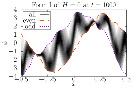
Figure 2: Waveform of $\phi$ obtained with Form I at $t=1000$ for $\Delta x=1/200$ and $\Delta t=1/1000$. The dashed and dotted lines are drawn with the even and odd numbers of grid points, respectively. On the other hand, the solid line is drawn with all grid points.

There are marked differences between the line with an even number of grid points and that with an odd number of grid points. These are mainly caused by the second-order difference formula in (9). This is explicitly expressed as

$$\delta^{ij}\widehat{\delta}^{\langle 1\rangle}_{i}\widehat{\delta}^{\langle 1\rangle}_{j}\phi^{(n)}_{(\boldsymbol{k})} =\sum_{i=1}^{n}\dfrac{\phi^{(n)}_{(k_{1},\dots,k_{i}+2,\dots,k_{n})}-2\phi^{(n)}_{(\boldsymbol{k})}+\phi^{(n)}_{(k_{1},\dots,k_{i}-2,\dots,k_{n})}}{(\Delta x^{i})^{2}}.$$

The expression indicates that the odd and even numbers of grid points are independent of each other. If the differences between the odd- and even-number grid points are generated by numerical errors, the grid points separate into those with even and odd numbers. On the other hand, the formula in (13) is explicitly expressed as

$$\delta^{ij}\widehat{\delta}^{\langle 2\rangle}_{ij}\phi^{(n)}_{(\boldsymbol{k})} =\sum_{i=1}^{n}\dfrac{\phi^{(n)}_{(k_{1},\dots,k_{i}+1,\dots,k_{n})}-2\phi^{(n)}_{(\boldsymbol{k})}+\phi^{(n)}_{(k_{1},\dots,k_{i}-1,\dots,k_{n})}}{(\Delta x^{i})^{2}}.$$

Thus, the odd- and even-number grid points are dependent on each other. If the differences are generated by numerical errors, the differences propagate at all grid points. Therefore, no vibrations occur in $\phi$ obtained with Form II as shown in Fig. 1.

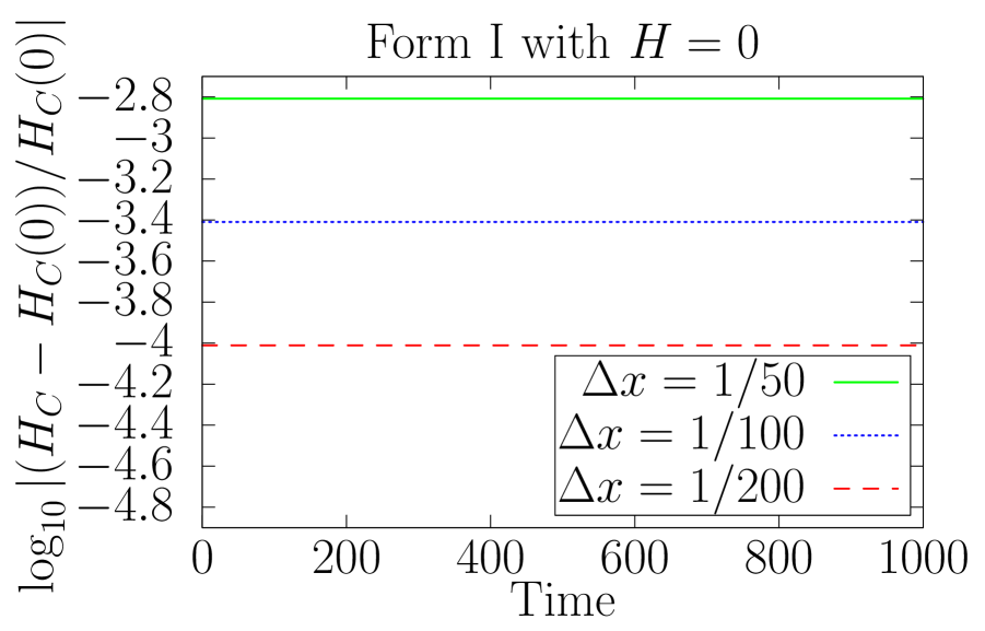
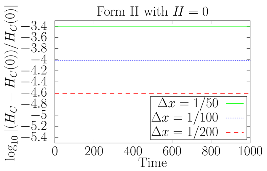
Figure 3: Relative errors of $H^{\mathrm{I}}_{C}$ against the initial value obtained with Form I and those of $H^{\mathrm{II}}_{C}$ against the initial value obtained with Form II in the Hubble constant as $H=0$. The left panel is drawn with Form I and the right one with Form II.

Fig. 3 shows relative errors of the discretized total Hamiltonians $H^{\mathrm{I}}_{C}$ and $H^{\mathrm{II}}_{C}$ against the initial value with Forms I and II, respectively. When the number of grid points is increased twofold, the value is about $0.6\approx\log_{10}4$ smaller in both panels. The results mean that $H^{\mathrm{I}}_{C}$ and $H^{\mathrm{II}}_{C}$ show the second-order accuracies with respect to the number of grid points. However, $H^{\mathrm{II}}_{C}$ should show the first-order accuracy because of the expression of (12). This discrepancy will be discussed in Sec. 5.

4.2 Curved spacetime

Next, we perform some simulations in an expanding space, that is, $H=10^{-3}$. The purpose of this study is to confirm the efficiency of the Hubble constant $H$ in terms of the accuracy and stability of the simulations. In Fig. 4, no vibrations appear. This has already been mentioned in [5], which means that the expansions of the space increase the stability of the simulations.

Figure 4: $\phi$ obtained with Forms I and II in $H=10^{-3}$. The left panel is drawn with Form I and the right one with Form II.

The modified total Hamiltonian $\tilde{H}_{C}$ is drawn in Fig. 5. At the initial time, the numerical accuracy is almost of the second order with respect to the grid. However, near $t=1000$, the accuracy is less than the second order. Therefore, the numerical accuracy decreases with time if $H\neq 0$.

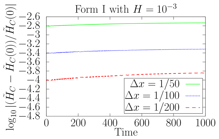
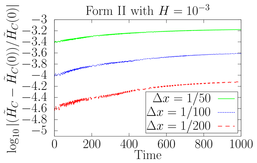
Figure 5: Relative errors of $\tilde{H}^{\mathrm{I}}_{C}$ against the initial value obtained with Form I and those of $\tilde{H}^{\mathrm{II}}_{C}$ against the initial value obtained with Form II in the Hubble constant as $H=10^{-3}$. The left panel is drawn with Form I and the right one with Form II.

5 Summary and discussion

We performed some simulations of the semilinear Klein–Gordon equation in the de Sitter spacetime with two structure-preserving discretized forms of the equation. Form I has the product of the first-order central difference formulae in the discretized evolution equations. Form II has the product of the first-order forward and backward difference formulae. If $H=0$, Form II is more stable than Form I because Form I but not Form II has numerical vibrations in the waveform. On the other hand, if $H=10^{-3}$, there are no vibrations in the waveform.

The numerical accuracies of the two forms are of the second order with respect to the grid if $H=0$. However, the expression of the total Hamiltonian of Form I indicates first-order accuracy.

In the construction from (2) to (12), the differential term in the one-dimensional case is

$$(\partial_{x}\phi)(\partial_{x}\phi) =\biggl{(}\dfrac{\phi^{(n)}_{(k+1)}-\phi^{(n)}_{(k)}}{\Delta x}-\dfrac{\Delta x}{2}\phi^{\prime\prime}+O((\Delta x)^{2})\biggr{)}^{2}+\biggl{(}\dfrac{\phi^{(n)}_{(k)}-\phi^{(n)}_{(k-1)}}{\Delta x}+\dfrac{\Delta x}{2}\phi^{\prime\prime}+O((\Delta x)^{2})\biggr{)}^{2}$$

$$=\biggl{(}\dfrac{\phi^{(n)}_{(k+1)}-\phi^{(n)}_{(k)}}{\Delta x}\biggr{)}^{2}+\biggl{(}\dfrac{\phi^{(n)}_{(k)}-\phi^{(n)}_{(k-1)}}{\Delta x}\biggr{)}^{2}-\phi^{\prime\prime}(\phi^{(n)}_{(k+1)}-2\phi^{(n)}_{(k)}+\phi^{(n)}_{(k-1)})+O((\Delta x)^{2})$$

$$=\biggl{(}\dfrac{\phi^{(n)}_{(k+1)}-\phi^{(n)}_{(k)}}{\Delta x}\biggr{)}^{2}+\biggl{(}\dfrac{\phi^{(n)}_{(k)}-\phi^{(n)}_{(k-1)}}{\Delta x}\biggr{)}^{2}+O((\Delta x)^{2}),$$

where we use the relation given by the evolution equation (13) such as

$$\phi^{(n)}_{(k+1)}-2\phi^{(n)}_{(k)}+\phi^{(n)}_{(k-1)} =(\Delta x)^{2}\biggl{[}\dfrac{\psi^{(n+1)}_{(k)}-\psi^{(n)}_{(k)}}{\Delta t}+m^{2}\phi^{(n)}_{(k)}+|\phi^{(n)}_{(k)}|^{p-1}\biggr{]}$$

$$=O((\Delta x)^{2}).$$

Therefore, we conclude that the relative errors of $H^{\mathrm{II}}_{C}$ obtained with Form II might affect the second-order accuracy with respect to the grid.

References

- [1] K. Yagdjian, The semilinear Klein–Gordon equation in de Sitter spacetime, Discrete Contin. Dyn. Syst. Ser. S 2 (3) (2009), 679–696.
- [2] M. Nakamura, The Cauchy problem for semilinear Klein–Gordon equations in de Sitter spacetime, J. Math. Anal. Appl. 410 (1) (2014), 445–454.
- [3] M. Nakamura, The Cauchy problem for the Klein–Gordon equation under the quartic potential in the de Sitter spacetime, J. Math. Phys. 62 (2021), 121509.
- [4] D. Furihata and T. Matsuo, Discrete Variational Derivative Method, CRC Press/Taylor & Francis, London, 2010.
- [5] T. Tsuchiya and M. Nakamura, On the numerical experiments of the Cauchy problem for semi-linear Klein–Gordon equations in the de Sitter spacetime, J. Comput. Appl. Math. 361 (2019), 396–412.
- [6] T. Tsuchiya and M. Nakamura, Numerical simulations of semilinear Klein–Gordon equations in the de Sitter spacetime with structure preserving scheme, Proceedings of the 13th ISAAC Congress (2022), in press.