Analysis and Detectability of Offline Data Poisoning Attacks on Linear Dynamical Systems

Abstract

In recent years, there has been a growing interest in the effects of data poisoning attacks on data-driven control methods. Poisoning attacks are well-known to the Machine Learning community, which, however, make use of assumptions, such as cross-sample independence, that in general do not hold for linear dynamical systems. Consequently, these systems require different attack and detection methods than those developed for supervised learning problems in the i.i.d. setting. Since most data-driven control algorithms make use of the least-squares estimator, we study how poisoning impacts the least-squares estimate through the lens of statistical testing, and question in what way data poisoning attacks can be detected. We establish under which conditions the set of models compatible with the data includes the true model of the system, and we analyze different poisoning strategies for the attacker. On the basis of the arguments hereby presented, we propose a stealthy data poisoning attack on the least-squares estimator that can escape classical statistical tests, and conclude by showing the efficiency of the proposed attack. The code can be found here https://github.com/rssalessio/data-poisoning-linear-systems.

1 Introduction

Over the past few decades, the rise in computational power, data accessibility, technological progress, and successful results have fueled research in data-driven methods. Nonetheless, these methods may be vulnerable to data poisoning attacks, which aim to degrade performance by altering the training data [Biggio et al.(2012)Biggio, Nelson, and Laskov, Barreno et al.(2006)Barreno, Nelson, Sears, Joseph, and Tygar, Barreno et al.(2010)Barreno, Nelson, Joseph, and Tygar]. The concept of poisoning was originally introduced for anomaly detection [Barreno et al.(2006)Barreno, Nelson, Sears, Joseph, and Tygar, Kloft and Laskov(2010), Rubinstein et al.(2009)Rubinstein, Nelson, Huang, Joseph, Lau, Rao, Taft, and Tygar] and attacks against SVM models [Biggio et al.(2012)Biggio, Nelson, and Laskov]. Thereafter, various machine learning models have been shown to be susceptible to poisoning attacks [Jagielski et al.(2018)Jagielski, Oprea, Biggio, Liu, Nita-Rotaru, and Li, Xiao et al.(2015)Xiao, Biggio, Brown, Fumera, Eckert, and Roli, Zhang et al.(2020)Zhang, Zhu, and Lessard, Shafahi et al.(2018)Shafahi, Huang, Najibi, Suciu, Studer, Dumitras, and Goldstein] (see also [Tian et al.(2022)Tian, Cui, Liang, and Yu] for a survey). In the field of systems control, data-driven methods are used due to a variety of reasons, such as decreased modeling complexity and/or reduced costs. In fact, data-driven control methods allow the user to formulate a control law directly from the data, thus bypassing the need of modeling the dynamical systems. There are a variety of these methods to use: techniques based on Willem’s et al. lemma [Willems et al.(2005)Willems, Rapisarda, Markovsky, and De Moor, De Persis and Tesi(2019), Coulson et al.(2019)Coulson, Lygeros, and Dörfler], Virtual Reference Feedback Tuning (VRFT) [Campi et al.(2002)Campi, Lecchini, and Savaresi], Iterative Feedback Tuning [Hjalmarsson(2002)], Correlation-based Tuning [Karimi et al.(2004)Karimi, Mišković, and Bonvin], etc. However, data-driven control methods may also be affected by poisoning attacks. In [Russo and Proutiere(2021)], the authors formulate a poisoning attack against the VRFT method. Similarly, in [Yu et al.(2022)Yu, Zhao, Chinchali, and Topcu] the authors propose a poisoning attack against data-driven predictive control methods. In [Showkatbakhsh et al.(2016)Showkatbakhsh, Tabuada, and Diggavi, Feng and Lavaei(2021)], the authors consider how to recover the underlying model of the system from poisoned data, while [Chekan and Langbort(2020)] considers enlarging the confidence set of the poisoned parameters to improve the performance of online LQR. The detection and analysis of these attacks, however, have received limited attention. Through first principles thinking, we investigate which models are compatible with the poisoned data. We focus on the least-squares (LS) estimator and study how poisoning affects the performance of this estimator. Through the lens of statistical tests, we examine how data can be poisoned and how these attacks can be detected. Our last contribution is to propose an attack that can impact the LS estimator while being stealthy to classical statistical tests, including residual and correlation tests typically used for anomaly detection. We provide examples and numerical simulations to accompany our results.

2 Related work

Data poisoning attacks can be categorized into two classes: untargeted poisoning attacks and targeted poisoning attacks [Tian et al.(2022)Tian, Cui, Liang, and Yu]. Attacks in the former class lead to some form of denial-of-service and try to hinder the convergence of the target model. On the other hand, targeted attacks change the data so that the trained model behaves according to the goal of the attacker [Liu et al.(2017)Liu, Ma, Aafer, Lee, Zhai, Wang, and Zhang, Shafahi et al.(2018)Shafahi, Huang, Najibi, Suciu, Studer, Dumitras, and Goldstein]. Countermeasures include preventive measures (e.g., encryption) or reactive measures (e.g., detection). In [Nguyen and Tran(2013), Bhatia et al.(2017)Bhatia, Jain, Kamalaruban, and Kar], the authors propose different techniques to recover a linear model from the data for oblivious adversaries, while for adaptive adversaries recovery is possible under some stringent assumptions [Bhatia et al.(2015)Bhatia, Jain, and Kar]. As mentioned in [Bhatia et al.(2017)Bhatia, Jain, Kamalaruban, and Kar], it seems unlikely that consistent estimators are even possible in face of a fully adaptive adversary.However, to the best of our knowledge, most of these techniques are not directly applicable to control problems, due to the underlying dynamics of the system. In [Alfeld et al.(2016)Alfeld, Zhu, and Barford], the authors study a targeted attack that poisons the forecasting of an autoregressive model. In [Showkatbakhsh et al.(2016)Showkatbakhsh, Tabuada, and Diggavi], the authors consider the problem of identifying a system whose output measurements have been corrupted by an adversary. They consider an omniscient adversary and given a bound on the number of attacked sensors, and some observability conditions, it is possible to derive a model that is useful for stabilizing the original system. A similar problem is studied in [Feng and Lavaei(2021)]: the authors consider a linear system affected by an unknown sparse adversarial disturbance $d_{t}$, and study how to recover the original model of the system. A different problem is studied in [Chekan and Langbort(2020)], where the authors consider online poisoning of the adaptive LQR method [Abbasi-Yadkori and Szepesvári(2011)], and, to compensate for the attack, they enlarge the confidence set of the estimator. In [Russo and Proutiere(2021)] they formulate a bi-level optimization problem to compute poisoning attacks against data-driven control methods. Their attack is then applied to the digital twin of a building to demonstrate the potential of their attack [Russo et al.(2021)Russo, Molinari, and Proutiere]. Lastly, in [Yu et al.(2022)Yu, Zhao, Chinchali, and Topcu] they extend the bi-level attack problem to attack data-driven predictive control methods.

3 Preliminaries

Model.

We consider a discrete-time LTI system affected by process noise:

$$x_{t+1}=A_{\star}x_{t}+B_{\star}u_{t}+w_{t},$$ (1)

where $t\in\mathbb{Z}$ is the discrete time variable, $x_{t}\in\mathbb{R}^{n}$ is the state of the system, $u_{t}\in\mathbb{R}^{m}$ is the control signal, $A_{\star}\in\mathbb{R}^{n\times n},B_{\star}\in\mathbb{R}^{n\times m}$ are the unknown system matrices, and $w_{t}\in\mathcal{W}\subseteq\mathbb{R}^{n}$ is an unmeasured disturbance belonging to some convex set $\mathcal{W}$ (which can be the entire $\mathbb{R}^{n}$). For a sequence of input-state measurements $\{u_{k}\}_{k=0}^{T-1},\{x_{k}\}_{k=0}^{T}$, we define $\psi_{t}=(x_{t}^{\top},u_{t}^{\top})^{\top}\in\mathbb{R}^{n+m}$ and the following data matrices:

$$X_{+}\coloneqq\begin{bmatrix}x_{1}&\dots&x_{T}\end{bmatrix},\quad X_{-}\coloneqq\begin{bmatrix}x_{0}&\dots&x_{T-1}\end{bmatrix},\quad U_{-}\coloneqq\begin{bmatrix}u_{0}&\dots&u_{T-1}\end{bmatrix},$$

and $X=\begin{bmatrix}x_{0}&\dots&x_{T}\end{bmatrix},\Psi_{-}=\begin{bmatrix}\psi_{0}&\dots&\psi_{T-1}\end{bmatrix}$. We make the assumption that the user has access to one trajectory of the system, used for identification or data-driven control.

Assumption 1

The data $\mathcal{D}=(U_{-},X)$ available to the user consists of one input-state trajectory of length $T$. Furthermore, the data satisfy the rank condition $\rank\Psi_{-}=n+m$.

This is a standard assumption in data-driven control, and it can be guaranteed for noise-free systems by choosing a persistently exciting input signal of order $n+1$ [Willems et al.(2005)Willems, Rapisarda, Markovsky, and De Moor].

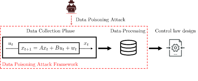
Figure 1: Data poisoning framework for data-driven control methods (figure adapted from [Russo and Proutiere(2021)]).

Data poisoning attacks.

We denote by $\Delta\mathcal{D}\coloneqq(\Delta U_{-},\Delta X)$ the poisoning signals on the input-state measurements, so that $\Delta U_{-}=\begin{bmatrix}\Delta u_{0}&\dots\Delta u_{T-1}\end{bmatrix}\in\mathbb{R}^{m\times T}$, $\Delta X=\begin{bmatrix}\Delta x_{0}&\dots\Delta x_{T}\end{bmatrix}\in\mathbb{R}^{n\times T+1}$. We let $\tilde{U}_{-}=U_{-}+\Delta U_{-}$, $\tilde{X}=X+\Delta X$ be the resulting poisoned signals. Similarly, we denote the poisoned dataset by ${\tilde{\mathcal{D}}}\coloneqq(\tilde{U}_{-},\tilde{X})$ and let $\tilde{\psi}_{t}=\psi_{t}+\Delta\psi_{t}$, where $\Delta\psi_{t}=(\Delta x_{t}^{\top},\Delta u_{t}^{\top})^{\top}$ (sim. we define $\tilde{\Psi}_{-}$, and $\Delta\Psi_{-}$). Attacks in the literature are generally classified as targeted attacks or untargeted attacks. Untargeted attacks just try to alter the performance of the data-driven control scheme, causing a denial-of-service. On the other hand, targeted attacks are usually carried out by the attacker to achieve some specific goals, e.g., making the closed-loop system unstable, maximizing the energy used by the system, making the system uncontrollable, etc. The attacker’s goal is formulated as a bi-level optimization problem (see also [Russo and Proutiere(2021)])

$$\max_{(\Delta U_{-},\Delta X)\in\mathcal{U}\times\mathcal{X}} \mathcal{A}\left(\mathcal{D},K\right)\textrm{ s.t. }K\in\operatorname*{arg\,min}_{K^{\prime}}\mathcal{L}(U_{-}+\Delta U_{-},X+\Delta X,K^{\prime}),$$ (2)

where $(\mathcal{U},\mathcal{X})$ is a convex set, $K$ is the closed-loop controller, $\mathcal{A}$ represents the objective function of the malicious agent, and $\mathcal{L}$ represents the function used by the victim to compute the control law $K$ according to the poisoned data $(\tilde{U}_{-},\tilde{X})$.

4 Attacks and Detection Strategies

In this section we examine what is the set of pairs $(A,B)$ that are compatible with the poisoned data ${\tilde{\mathcal{D}}}$, and establish a sufficient and necessary condition for $(A_{\star},B_{\star})$ to be compatible with ${\tilde{\mathcal{D}}}$. We investigate how least-squares estimate changes under poisoning, examine attack detection, and propose a stealthy untargeted attack on the least-squares estimate.

4.1 The set of compatible models under data poisoning

Most data-driven control methods assume that there exists a linear system $(A,B)$ that is consistent with the data. Ignoring the noise term $w_{t}$ in eq. 1, consistency amounts to finding all $(A,B)\in\mathbb{R}^{n\times(n+m)}$ that satisfy the equation $X_{+}=AX_{-}+BU_{-}$ (i.e., all the pairs consistent with the dataset). In presence of a noise signal $w_{t}$, consistency is derived from the following relationship

$$\begin{bmatrix}I_{n}&-A_{\star}&-B_{\star}\end{bmatrix}\begin{bmatrix}X_{+}\\ \Psi_{-}\end{bmatrix}=W_{-},$$ (3)

where $W_{-}=\begin{bmatrix}w_{0}&w_{1}&\dots&w_{T-1}\end{bmatrix}\in\mathcal{W}^{T}$ (where $\mathcal{W}^{T}\coloneqq\bigtimes_{n=1}^{T}\mathcal{W}$). Then, given a poisoned dataset $\tilde{\mathcal{D}}=(\tilde{U}_{-},\tilde{X})$, we wonder for which $(A,B)\in\mathbb{R}^{n\times(n+m)}$ and $\tilde{W}\in\mathcal{W}^{T}$ the following relationship holds

$$\begin{bmatrix}I_{n}&-A&-B\end{bmatrix}\begin{bmatrix}\tilde{X}_{+}\\ \tilde{\Psi}_{-}\end{bmatrix}=\tilde{W}_{-}.$$ (4)

To answer this question, we seek the set of noise sequences $\mathcal{W}_{\tilde{\mathcal{D}}}$ that are compatible with the data ${\tilde{\mathcal{D}}}$. Following a similar approach as in [Koch et al.(2020)Koch, Berberich, and Allgöwer], we note that the compatible noise terms $\{\tilde{w}_{t}\}_{t}$ belong to the image of $\tilde{G}\coloneqq\begin{bmatrix}\tilde{X}_{+}^{\top}&\tilde{\Psi}_{-}^{\top}\end{bmatrix}^{\top}$. Straightforwardly, if $\tilde{W}_{-}\tilde{G}^{\perp}=0$, then $\tilde{W}_{-}$ is compatible with the data (where $\tilde{G}^{\perp}$ denotes a basis of the kernel of $\tilde{G}$), and $\mathcal{W}_{{\tilde{\mathcal{D}}}}$ is

$$\mathcal{W}_{{\tilde{\mathcal{D}}}}=\left\{\tilde{W}_{-}\in\mathcal{W}^{T}:\tilde{W}_{-}\tilde{G}^{\perp}=0\right\}.$$ (5)

Therefore, the following result characterizes in which cases $(A_{\star},B_{\star})\in\Sigma_{{\tilde{\mathcal{D}}}}$.

Lemma 4.1.

Consider a poisoned dataset ${\tilde{\mathcal{D}}}$. The set of all pairs $(A,B)$ that are consistent with the data ${\tilde{\mathcal{D}}}$ is $\Sigma_{\tilde{\mathcal{D}}}\coloneqq\left\{(A,B)\in\mathbb{R}^{n\times n+m}:\exists\tilde{W}_{-}\in\mathcal{W}_{\tilde{\mathcal{D}}}:(\ref{eq:fundamental_eq_poisoned_system_simplified})\hbox{ holds for }(A,B,\tilde{W}_{-})\right\}.$ Let $\tilde{W}_{\star}=W_{-}+\Delta W_{-}$, where $\Delta W_{-}=\Delta X_{+}-A_{\star}\Delta X_{-}-B_{\star}\Delta U_{-}$. Then $(A_{\star},B_{\star})\in\Sigma_{{\tilde{\mathcal{D}}}}\iff\tilde{W}_{\star}\in\mathcal{W}^{T}.$

In most applications, $\mathcal{W}$ is considered to be $\mathbb{R}^{n}$ itself, which essentially guarantees that $(A_{\star},B_{\star})\in\Sigma_{\tilde{\mathcal{D}}}$. However, if the disturbance $\{w_{t}\}_{t\geq 0}$ is generated according to some probability measure $\mathbb{P}$, then the likelihood of $\tilde{W}_{\star}$ may be small under $\mathbb{P}$ depending on the attack. In other applications, $\mathcal{W}$ is a known bounded convex set, and may not contain the sequence $\tilde{W}_{\star}$. In this case, it is necessary to enlarge $\mathcal{W}$ to be able to recover the original model. Lastly, in some scenarios the user may know in advance an over-approximate $\hat{\Sigma}_{\mathcal{D}}$ of $\Sigma_{\mathcal{D}}$, which can be used to infer if the data has been poisoned in case $\hat{\Sigma}_{\mathcal{D}}$ and $\Sigma_{\tilde{\mathcal{D}}}$ are too different (using, for example, Bayesian hypothesis testing).

This result can also be interpreted in the following way: if $\mathcal{W}$ is a bounded convex set, an attacker may try to bound $\Delta X$ and $\Delta U_{-}$ to bound $\Delta W_{-}$, and, consequently, act on the compatibility of the true system matrices. Obviously, upper bounding the norm of the poisoning signals seems like a good way to make sure that is less detectable. However, just bounding the norm of the poisoning signals, as we see in the forthcoming sections, is not enough to achieve undetectability of an attack.

4.2 Attack strategies for the least-squares estimator

To better understand how to formulate attack strategies, and analyze the problem of detectability, we now turn our attention to the least-squares (LS) estimator. As pointed out in [De Persis and Tesi(2019)], this LS estimate is used in the formulation of data-driven controllers. The unpoisoned LS estimate can be compactly written as $(A_{\textrm{LS}},B_{\textrm{LS}})=X_{+}\Psi_{-}^{\dagger}$ ($\Psi_{-}^{\dagger}$ is the right inverse of $\Psi_{-}$). We also denote by $(A_{\textrm{LS}},B_{\textrm{LS}})$ and $(\tilde{A}_{\textrm{LS}},\tilde{B}_{\textrm{LS}})$ the LS estimates when, respectively, $\mathcal{D}$ and ${\tilde{\mathcal{D}}}$ are used. Furthermore, let $(\Delta\tilde{A}_{\textrm{LS}},\Delta\tilde{B}_{\textrm{LS}})=(\tilde{A}_{\textrm{LS}}-A_{\star},\tilde{B}_{\textrm{LS}}-B_{\star})$ the difference between the LS estimate and the true parameter, and indicate by $\Delta\tilde{\theta}_{\textrm{LS}}=\operatorname{vec}(\Delta\tilde{A}_{\textrm{LS}},\Delta\tilde{B}_{\textrm{LS}})$ its vectorization. We further assume that $\rank\tilde{\Psi}_{-}=n+m$. In presence of a poisoning attack $(\Delta X,\Delta U_{-})$ we obtain the following straightforward result, which is used to discuss possible attack strategies.

Lemma 4.2.

The LS error is given by $(\Delta\tilde{A}_{\textrm{LS}},\Delta\tilde{B}_{\textrm{LS}})=\tilde{W}_{\star}\tilde{\Psi}_{-}^{\dagger},$ where $\tilde{W}_{\star}$ is as in lemma 4.1. In addition to that, we have $\sigma_{\text{min}}(W_{-})+\sigma_{\text{min}}(\Delta W_{-})\leq\|\tilde{\Psi}_{-}\|_{\textnormal{F}}\|\Delta\tilde{\theta}_{\textrm{LS}}\|_{2}\leq\sigma_{\text{max}}(W_{-})+\sigma_{\text{max}}(\Delta W_{-})$, where $\|\cdot\|_{\textnormal{F}}$ indicates the Frobenius norm and $\sigma_{\text{min}},\sigma_{\text{max}}$ the minimum and maximum singular values.

Relationship between poisoning and exploration.

This result provides a way to formulate possible attack strategies and to analyze their impact. The adversary clearly needs to minimize the amount of exploration, quantified by the term $\|\tilde{\Psi}_{-}\|_{\textnormal{F}}=\sum_{t=0}^{T-1}\|\tilde{\psi}_{t}\|_{2}$ to maximize the error. Fundamentally, any attack wishing to maximize the error needs to change the data as to minimize the exploration performed by the victim. As an informal argument, define $\tilde{C}_{T}=\sum_{t=0}^{T-1}(\tilde{\psi}_{t}\otimes I_{n})(\tilde{\psi}_{t}\otimes I_{n})^{\top}$ and introduce the unexcitation subspace $\tilde{\mathcal{U}}=\left\{\theta\in\mathbb{R}^{n(n+m)}:\lim\sup_{T\to\infty}\theta^{\top}\tilde{C}_{T}\theta<\infty\right\}$ (see [Bittanti et al.(1992)Bittanti, Campi, and Lorito]), and let $\tilde{\mathcal{E}}$ be its orthogonal complement (the data generation process is undefined on purpose, since it is just an illustrative argument). Denote by $\Delta\tilde{\theta}_{\textrm{LS}}^{\tilde{\mathcal{E}}}$ and $\Delta\tilde{\theta}_{\textrm{LS}}^{\tilde{\mathcal{U}}}$ the orthogonal projections of $\Delta\tilde{\theta}_{\textrm{LS}}$ on these two subspaces, so that $\Delta\tilde{\theta}_{\textrm{LS}}=\Delta\tilde{\theta}_{\textrm{LS}}^{\tilde{\mathcal{E}}}+\Delta\tilde{\theta}_{\textrm{LS}}^{\tilde{\mathcal{U}}}$. Then, under some simple assumptions, it is possible to show that asymptotically $\|\Delta\tilde{\theta}_{\textrm{LS}}\|_{2}=\|\Delta\tilde{\theta}_{\textrm{LS}}^{\tilde{\mathcal{U}}}\|_{2}$. Hence, maximizing $\|\Delta\tilde{\theta}_{\textrm{LS}}\|$ amounts to changing the unpoisoned regressor $\psi_{t}$ so that, the unexcitation subspace becomes ”larger”, which implies that the amount of exploration is lowered. To formalize the concept, let $\{v_{i}\}_{i=1}^{n(n+m)}$ be an orthonormal basis of $\mathbb{R}^{n(n+m)}$ with $v_{1}=\theta_{\textrm{LS}}/\|\theta_{\textrm{LS}}\|_{2}$, where $\theta_{\textrm{LS}}=\operatorname{vec}(A_{\textrm{LS}},B_{\textrm{LS}})$ is the true LS-estimate for an unpoisoned dataset. Then, the estimation error in the direction of $v_{k}$ is given by $|v_{k}^{\top}\Delta\tilde{\theta}_{\textrm{LS}}|$, which is lower bounded as follows.

Corollary 4.3.

For any $k=1,\dots,n(n+m)$, and a poisoned dataset ${\tilde{\mathcal{D}}}$

$$\sqrt{(v_{k}^{\top}\Delta\tilde{\theta}_{\textrm{LS}})^{2}}\geq\frac{|\cos(\alpha_{k})|(\sigma_{\text{min}}(W_{-})+\sigma_{\text{min}}(\Delta W_{-}))}{\|V_{k}\tilde{\Psi}_{-}\|_{\textnormal{F}}},$$ (6)

where $V_{k}=\operatorname{vec}_{n,n+m}^{-1}(v_{k})$, and $\alpha_{k}$ is the angle between $\operatorname{vec}(V_{k}\tilde{\Psi}_{-})$ and $\operatorname{vec}(\tilde{W}_{\star})$.

The term $\|V_{k}\tilde{\Psi}_{-}\|_{\textnormal{F}}$ can be interpreted as the total amount of exploration in the direction of $v_{k}$. Minimizing the exploration in the direction of the true estimate $\theta_{\textrm{LS}}$ implies a larger value of $|v_{1}^{\top}\Delta\tilde{\theta}_{\textrm{LS}}|$, which is larger when the estimator error $\Delta\tilde{\theta}_{\textrm{LS}}$ is parallel to $\theta_{\textrm{LS}}$, from which we deduce that asymptotically the unexcitation subspace includes the unpoisoned estimate $\theta_{\textrm{LS}}$.

These results not only shed a light on the mechanics of poisoning, but also help us define a possible attack. The attacker can compute some poisoning signals $(\Delta X,\Delta U_{-})$ by solving the convex problem $\min_{(\Delta X,\Delta U_{-})\in\mathcal{C}}\|\tilde{\Psi}_{-}\|_{\textnormal{F}}$ (or $\min_{(\Delta X,\Delta U_{-})\in\mathcal{C}}\|V_{1}\tilde{\Psi}_{-}\|_{\textnormal{F}}$), where $\mathcal{C}$ is some convex set. Nevertheless, this simple attack ignores other terms, such as $\Delta W_{-}$, and therefore may not be enough to significantly impact the LS estimate. As we discuss in the next sections, maximizing the norm of the LS residuals fills this gap. Furthermore, as we see, an attacker needs to impose additional constraints on the optimization problem to make an attack stealthy. To that aim, we begin by discussing how statistical hypothesis testing can help to detect poisoning attacks.

4.3 Detection analysis for the LS estimator

The detection of any attack should be based on two important ingredients: (1) prior knowledge of the system and its signals; (2) independent statistical tests. Prior knowledge is useful to detect possible wrongdoings, however, that knowledge may be biased. Therefore, it is important to complement tests based on prior knowledge with tests that are independent of that knowledge. Prior knowledge, for example, includes confidence bounds on the variance of the noise and/or knowledge of the statistical properties of $\{(x_{t},u_{t})\}_{t}$. If any of those are known, it is possible to derive one-sample tests to assess these statistics.In the following, we relate poisoning attacks to classical statistical tests. We begin our study by considering attacks on the input signal, and then consider attacks on the state signal as well.

4.3.1 Detection of Attacks on the input signal

The statistical properties of the input signal are usually assumed to be known. In fact, in most experiments, the input is usually chosen as a white noise signal, as to excite the dynamics of the system. Assuming $\{u_{t}\}_{t}$ is a sequence of i.i.d. random variables with distribution $P$, whiteness tests [Box et al.(2015)Box, Jenkins, Reinsel, and Ljung, Drouiche(2000)] can be used to deduce if the samples in $\{\tilde{u}_{t}\}_{t}$ are white, while one-sample tests (such as the Kolmogorov-Smirnov test [Massey Jr(1951)], or the Anderson-Darling test [Nelson(1998)]) can be used to assess whether the samples in $\{\tilde{u}_{t}\}_{t}$ are distributed according to $P$. More simply, if $u_{t}\sim\mathcal{N}(0,I_{m})$, then $\|U_{-}\|_{\textnormal{F}}^{2}\sim\chi^{2}(Tm)$ is a Chi-squared distribution with $Tm$ degrees of freedom. Consequently, for a small $\delta\geq 0$ we see the constraint $\|\Delta U_{-}\|_{\textnormal{F}}\leq\delta\|U_{-}\|_{\textnormal{F}}$ as a way to constraint the Chi-squared statistics. Along this reasoning, an important class of input attacks can be derived when $(u_{t},\tilde{u}_{t})$ are indistinguishable, i.e., statistically equivalent.

Definition 4.4.

Suppose that $u_{t}$ is i.i.d., distributed according to $P$ for every $t\geq 0$. Then, $(u_{t},\tilde{u}_{t})$ are indistinguishable if $\tilde{u}_{t}$ is i.i.d. and distributed according to $P$ for every $t\geq 0$.

To illustrate the attack, consider the following example.

Example 4.5.

Consider the system $x_{t+1}=a_{\star}x_{t}+b_{\star}u_{t}+w_{t}$, with $(a_{\star},b_{\star})=(0.7,0.5)$ and $w_{t}\sim\mathcal{N}(0,1)$. In fig. 2 are shown the confidence intervals for the LS estimate when the input has been poisoned according to the indistinguishable attack $\tilde{u}_{t}$, where $(u_{t},\tilde{u}_{t})$ are independent, i.i.d., and distributed according to $\mathcal{N}(0,1)$. Under poisoning, the estimate of $b_{\star}$ converges to $0$ as $T\to\infty$.

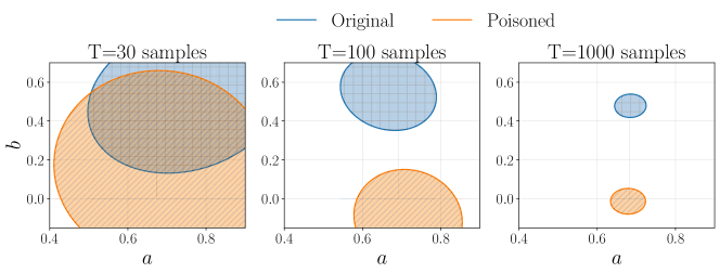
Figure 2: Example of input poisoning (see example 4.5). The colored ellipses depict the 95% confidence interval of the LS estimates of the true parameters $(a_{\star},b_{\star})$. When the input data is poisoned, we obtain an $F$-statistic of $Z_{\tilde{\mathcal{D}}}\approx(0.45,0.62,0.15)$ respectively for $T=(15,100,1000)$ samples. Otherwise, we obtain $Z_{\mathcal{D}}\approx(7.35,29.05,233.35)$.

This insight leads us to the following result.

Lemma 4.6.

Let $\{u_{t}\}_{t=0}^{T-1}$ be an i.i.d. sequence distributed according to $\mathcal{N}(0,\Sigma_{u})$. Assume $\Delta u_{t}=-u_{t}+a_{t}$ to be an indistinguishable attack, with $a_{t}\sim\mathcal{N}(0,\Sigma_{u})$ independent of $u_{t}$, and $\Delta x_{t}=0,t\geq 0$. Then, if $A$ is stable, $\Delta\tilde{B}_{\textrm{LS}}\to-B_{\star}$ w.p. $1$ as $T\to\infty$.

Intuitively, if the poisoned input is completely uncorrelated from the data, then the best estimate of $B_{\star}$ is $0$. Simply, as the number of samples grows larger, $B_{\star}+\Delta\tilde{B}_{\textrm{LS}}\to 0$.

To detect this type of attack, we propose to test the explanatory power of the input data. Using classical partial $F$-tests [Kleinbaum et al.(2013)Kleinbaum, Kupper, Nizam, and Rosenberg], we test the hypothesis $H_{0}:\|B_{\star}\|=0$ against $H_{1}:\|B_{\star}\|\neq 0$. Assume the underlying system is affected by some process noise $w_{t}\sim\mathcal{N}(0,\Sigma_{w})$. Denote by $\tilde{A}^{(1)}_{\textrm{LS}}$ the LS estimate of $A_{\star}$ when the input signal $\tilde{u}_{t}$ is not used by the LS estimator. Similarly, denote by $(\tilde{A}^{(2)}_{\textrm{LS}},\tilde{B}^{(2)}_{\textrm{LS}})$ the LS estimate when $\tilde{u}_{t}$ is considered in the estimation process. Consider the LS residuals, and define the statistic

$$Z_{\tilde{\mathcal{D}}}\coloneqq\frac{\left\lVert X_{+}-\tilde{A}^{(1)}_{\textrm{LS}}X_{-}\right\rVert_{\textnormal{F}}^{2}-\left\lVert X_{+}-\tilde{A}^{(2)}_{\textrm{LS}}X_{-}+\tilde{B}^{(2)}_{\textrm{LS}}\tilde{U}_{-}\right\rVert_{\textnormal{F}}^{2}}{(nm/(T-n(n+m)-1))\left\lVert X_{+}-\tilde{A}^{(2)}_{\textrm{LS}}X_{-}+\tilde{B}^{(2)}_{\textrm{LS}}\tilde{U}_{-}\right\rVert_{\textnormal{F}}^{2}}.$$ (7)

Under $H_{0}$ it can be shown that the statistics $Z_{\tilde{\mathcal{D}}}$ follows an $F$ distribution with $(nm,T-n(n+m)-1)$ degrees of freedom (follows from an application of [Ljung(1998), Lemma II.4]). Using this partial $F$-test, we reject $H_{0}$ if and only if $Z_{\tilde{\mathcal{D}}}>f_{nm,T-n(n+m)-1}^{\alpha}$, where $f_{a,b}^{\alpha}$ is the upper $\alpha$-point of an $F$ distribution with $(a,b)$ degrees of freedom. In conclusion, not rejecting $H_{0}$ may indicate that the input data has been poisoned. Clearly, for more complex cases, we need to resort to other tools, such as the analysis of the residuals, as explained in the following section.

4.3.2 Residual analysis

We claim that any attacker that wishes to remain stealthy needs to make sure that the residuals of the LS procedure satisfy certain statistical conditions. We begin by deriving the following bound on the residuals of the LS estimate for generic attacks that are independent of the noise signal $\{w_{t}\}_{t}$ (this includes the class of oblivious attacks). Let the residual of $(\tilde{A}_{\textrm{LS}},\tilde{B}_{\textrm{LS}})$ at time $t$ be $\tilde{R}_{t}=\tilde{x}_{t+1}-\tilde{A}_{\textrm{LS}}\tilde{x}_{t}-\tilde{B}_{\textrm{LS}}\tilde{u}_{t}$. In matrix notation, we write $\tilde{R}=\begin{bmatrix}\tilde{R}_{0}&\tilde{R}_{1}&\dots&\tilde{R}_{T-1}\end{bmatrix}=\tilde{X}_{+}-\begin{bmatrix}\tilde{A}_{\textrm{LS}}&\tilde{B}_{\textrm{LS}}\end{bmatrix}\tilde{\Psi}_{-}$ (similarly, we denote by $R$ the residuals in absence of poisoning).

Lemma 4.7.

Assume $\{(\Delta x_{t},\Delta u_{t})\}_{t}$ to be independent of the i.i.d. noise sequence $\{w_{t}\}_{t}$, with $w_{t}\sim\mathcal{N}(0,\Sigma_{w})$. Then, the MSE $\mathbb{E}\left[\|\tilde{R}\|_{\textnormal{F}}^{2}\right]$ satisfies $0\leq\mathbb{E}\left[\|\tilde{R}\|_{\textnormal{F}}^{2}-\left\lVert R\right\rVert_{\textnormal{F}}^{2}\right]\leq\mathbb{E}[\sum_{i}\sigma_{i}^{2}(\Delta W_{-})]$, where $\sigma_{i}$ is the i-th singular value. Furthermore, $\|R\|_{\textnormal{F}}^{2}$ is a quadratic form of a normal random vector, distributed according to $\sum_{i=1}^{n}\lambda_{i}\chi^{2}(T-n-m)$, with $\lambda_{i}$ being the $i$-th eigenvalue of $\Sigma_{w}$.

As a corollary, for oblivious random attacks, we find that if $\Delta x_{t}\sim\mathcal{N}(0,\Sigma_{\Delta x})$ and $\Delta u_{t}\sim\mathcal{N}(0,\Sigma_{\Delta u})$ are i.i.d., then the previous result can be improved as follows $\mathbb{E}\left[\|\tilde{R}\|_{\textnormal{F}}^{2}-\|R\|_{\textnormal{F}}^{2}\right]=(T-n-m)\left[Tr\left(\Sigma_{\Delta x}+A_{\star}\Sigma_{\Delta x}A_{\star}^{\top}+B_{\star}\Sigma_{\Delta u}B_{\star}^{\top}\right)\right],$ with $\|\tilde{R}\|_{\textnormal{F}}^{2}\sim\sum_{i=1}^{n}\bar{\lambda}_{i}\chi^{2}(T-n-m)$, and $\bar{\lambda}_{i}$ is the i-th eigenvalue of $\Sigma_{\Delta x}+A_{\star}\Sigma_{\Delta x}A_{\star}^{\top}+B_{\star}\Sigma_{\Delta u}B_{\star}^{\top}+\Sigma_{w}$. This result also applies to the class of indistinguishable input attacks previously explained and motivates why in example 4.5 the confidence region in the poisoned case is significantly larger than in the unpoisoned one (due to the larger variance). In addition, observe the following lemma on the sensitivity of the residuals.

Lemma 4.8 (Sensitivity).

For any fixed attack satisfying the rank condition $\rank\tilde{\Psi}_{-}=n+m$, we obtain the following sensitivity on the residuals $\frac{\|\tilde{R}-R\|_{\textnormal{F}}}{\|R\|_{\textnormal{F}}}\leq\|\Delta\Psi_{-}\|_{2}\|\tilde{\Psi}_{-}\|_{\textnormal{F}}^{-1}$.

Lemma 4.7 and 4.8 link the problem of maximizing the LS error to that of minimizing the amount of exploration $\|\tilde{\Psi}_{-}\|_{\textnormal{F}}$ (as discussed in sec. 4.2) as well as maximizing the singular values of $\Delta W_{-}$. Furthermore, Lemma 4.7 can be used to formulate a possible detection test on the variance of the residuals. In fact, we note that any attack independent of the noise will necessarily increase the variance of the residuals. This observation provides us a hint to test the variance of the residuals. It is possible to derive a two-tail test on the variance of the residuals (as long as the user knows has some knowledge on the covariance of the noise) to verify that the data has not been poisoned. The user can test whether $\|\tilde{R}\|_{\textnormal{F}}^{2}$ belongs to the range $Q_{(1-\alpha)/2,T-n-M}(\lambda_{1},\dots,\lambda_{n})\leq\|\tilde{R}\|_{\textnormal{F}}^{2}\leq Q_{\alpha/2,T-n-M}(\lambda_{1},\dots,\lambda_{n}),$ where $Q_{x,d}(\lambda_{1},\dots)$ is the critical value of the distribution $\sum_{i=1}^{n}\lambda_{i}\chi^{2}(d)$ with significance $x\in(0,1)$. If the values of $\lambda_{1},\dots,\lambda_{n}$ are known to belong to some confidence region, the user can perform a Bayesian likelihood ratio test. Before we continue with an example, consider that the assumption of independence between $(\Delta U_{-},\Delta X)$ and $W_{-}$ may not be always satisfied: if the attacker has access to the dataset $\mathcal{D}$, then it is likely that she uses $X$, which depends on $W_{-}$, to compute the attack vector $(\Delta U_{-},\Delta X)$. In other cases, for example, when the attacker has limited capabilities on the dataset and/or the poisoned sensors, the assumption of independence is more likely to hold. Similarly, the assumption holds whenever the attacker is executing an attack that has been computed on a different set of data. Moreover, from simulations, it seems that this test is still valid to detect a possible adaptive attack.

Example 4.9 (Untargeted attack).

Consider an attacker that maximizes the norm of the residuals $\|\tilde{R}\|_{\textrm{F}}$ as a proxy to maximize $\left\lVert\begin{bmatrix}\Delta\tilde{A}_{\textrm{LS}}&\Delta\tilde{B}_{\textrm{LS}}\end{bmatrix}\right\rVert_{2}$. Let $\delta\geq 0$ be a parameter that limits the amplitude of the poisoning signals, and define $\Delta\tilde{W}_{-}\coloneqq\Delta X_{+}-A_{\textrm{LS}}\Delta X_{-}-B_{\textrm{LS}}\Delta U_{-}$. Then, as detailed in the appendix, the adversary can solve the following concave problem to compute an attack:

$$\max_{\Delta U_{-},\Delta X} Tr\left((\Delta\tilde{W}_{-}+2R)\Delta\tilde{W}_{-}^{\top}\right)\quad\textrm{s.t.}\quad\|\Delta X\|_{\textnormal{F}}\leq\delta\|X\|_{\textnormal{F}},\|\Delta U_{-}\|_{\textnormal{F}}\leq\delta\|U_{-}\|_{\textnormal{F}}.$$ (8)

Consider the $4$-dimensional system used in [Russo and Proutiere(2021)], affected by white noise with standard deviation $\sigma_{w}=0.1$. The victim has collected $T=200$ samples using $u_{t}\sim\mathcal{N}(0,1)$. In fig. 3 are shown the results when $(\ref{eq:untargeted_attack_maximize_mse_error})$ is solved using (1) convex-concave programming (CCP), (2) the cross-entropy method [De Boer et al.(2005)De Boer, Kroese, Mannor, and Rubinstein] and (3) random sampling from a Gaussian distribution (check the appendix for details). Note that the attacks can be easily detected for small values of $\delta$ using the test on the residuals (central plot). On the right plot, observe that, as discussed after corollary 4.3, the vectors $\theta_{\textrm{LS}}$ and $\Delta\tilde{\theta}_{\textrm{LS}}$ tend to align with each other when the attack is impactful.

Figure 3: Untargeted attack that maximizes the MSE. The curves indicate an average and its 95% confidence interval over 100 runs. From left to right : (1) impact on the LS estimate; (2) the p-value (right-tail) under the assumption of white noise with $\sigma_{w}=0.1$; (3) the angle between the unpoisoned estimate $\theta_{\textrm{LS}}$ and the error of the poisoned estimate $\Delta\tilde{\theta}_{\textrm{LS}}$.

This last example indicates that minimizing the norm of the poisoning signal is not enough to minimize detectability. Even though the poisoned signal and the unpoisoned one are similar, maximizing the MSE greatly affects the distribution of the residuals. Thereby, it may be more beneficial for the adversary to directly maximize $\|\begin{bmatrix}\Delta\tilde{A}_{\textrm{LS}}&\Delta\tilde{B}_{\textrm{LS}}\end{bmatrix}\|_{2}$ (which is a non-convex problem), while constraining the residuals of the models, to decrease detectability. A hint comes from the fact that the noise term at time $t$ is $\tilde{w}_{t}=w_{t}+\Delta w_{t}=w_{t}+\Delta x_{t+1}-A_{\star}\Delta x_{t}-B_{\star}\Delta u_{t}$. Since the noise $\tilde{w}_{t}$ depends on $\Delta x_{t+1}$, the victim can expect to observe a large value in the correlation of the residuals at lag $1$. This last observation suggests that an adversary may consider constraining the correlation of the residuals to reduce the detectability.

Correlation tests.

Consider white process noise $w_{t}\sim\mathcal{N}(0,\Sigma_{w})$, and let $\tilde{C}_{\tau}=\frac{1}{T}\sum_{t=0}^{T-\tau-1}\tilde{R}_{t}\tilde{R}_{t+\tau}^{\top}$ be the sample correlation of the residuals at lag $\tau$. Under the null hypothesis that the data has not been poisoned, asymptotically we obtain $\sqrt{T}\operatorname{vec}C_{\tau}\sim\mathcal{N}(0,\Sigma_{w}\otimes\Sigma_{w})$ (from an application of [Ljung(1998), Lemma 9.A1]), from which we derive the statistics $T\|C_{\tau}C_{0}^{-1}\|_{\textnormal{F}}^{2}\sim\chi^{2}(n^{2})$. Similarly, following a similar approach as in [Hosking(1980)], it is possible to derive the asymptotic Portmanteau statistics to test the whiteness of the residuals $T\sum_{\tau=1}^{T}\|C_{\tau}C_{0}^{-1}\|_{\textnormal{F}}^{2}\sim\chi^{2}(n^{2}(T-n-m))$. Using these statistics, it is possible to formulate a stealthy attack, as explained in the next section.

4.4 Stealthy untargeted attack

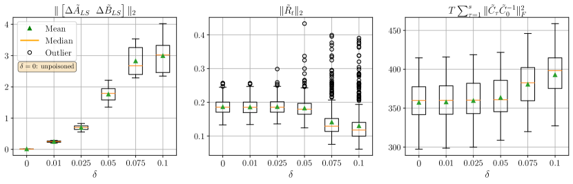
Figure 4: Stealthy attacks on the system used in example 4.9. From left to right: distribution over 10 different seeds of the impact on the LS error, $\|\tilde{R}_{t}\|_{2}$ and $T\sum_{\tau=1}^{s}\|\tilde{C}_{\tau}\tilde{C}_{0}^{-1}\|_{\textrm{F}}^{2}$.

On the basis of the previous findings, we argue that the main quantities of interest to make a poisoning attack stealthy are (1) the norm of the poisoning signals; (2) $\|\tilde{R}\|_{\textnormal{F}}^{2}$ the norm of the residuals; (3) $\|\tilde{C}_{\tau}\tilde{C}_{0}^{-1}\|_{\textnormal{F}}^{2},\tau=1,\dots,T-1,$ the norm of the self-normalized correlation terms. Consequently, we propose the following optimization problem to compute poisoning stealthy untargeted attacks:

$$\max_{\Delta U_{-},\Delta X} \left\lVert\begin{bmatrix}\Delta\tilde{A}_{\textrm{LS}}&\Delta\tilde{B}_{\textrm{LS}}\end{bmatrix}\right\rVert_{2}\textrm{ s.t. }g_{i}(\mathcal{D},\Delta U,\Delta X)\leq\delta_{i},\quad i=0,2,\dots,s+3,$$ (9)

with $g_{0}=\|\Delta X\|_{\textnormal{F}}/\|X\|_{\textnormal{F}}$, $g_{1}=\|\Delta U\|_{\textnormal{F}}/\|U\|_{\textnormal{F}}$, $g_{2}=\left|1-\|\tilde{R}\|_{\textnormal{F}}^{2}/\|R\|_{\textnormal{F}}^{2}\right|$, $g_{3}=|1-Z_{\tilde{\mathcal{D}}}/Z_{\mathcal{D}}|$ and $g_{3+\tau}=\left|1-\|\tilde{C}_{\tau}\tilde{C}_{0}^{-1}\|_{\textnormal{F}}^{2}/\|C_{\tau}C_{0}^{-1}\|_{\textnormal{F}}^{2}\right|,\tau=1,\dots,s$, for some $s<T-1$. Intuitively, the constraints limit the relative change of each quantity.

Numerical results.

We applied the attack resulting from (9) on the system used in example 4.9, with $T=500$, $s=25$ and the same value of $\delta$ for all constraints. Since $n=4,m=1$, there are $2504$ variables to optimize. The optimization problem is non-convex, therefore a local solution can be found by means of first-order methods. Results (see fig. 4 and other figures in the appendix) indicate that the resulting poisoning signals can relevantly impact the LS estimate, while the statistical indicators (central and right plot in fig. 4) show no evidence of anomaly. Furthermore, the attack seems to impact have a greater impact on the estimate of $A_{\textrm{LS}}$ than that of $B_{\textrm{LS}}$ (see also the appendix; for $\delta=0.05$ we obtain $\mathbb{E}\|\Delta\tilde{A}_{\textrm{LS}}\|_{2}\approx 2$ and $\mathbb{E}\|\Delta\tilde{B}_{\textrm{LS}}\|_{2}\approx 0.15$). Preliminary results indicate that this effect may be due to the presence of the constraint $g_{3}$ on $(\mathcal{Z}_{\tilde{\mathcal{D}}},\mathcal{Z}_{\mathcal{D}})$. Lastly, we observe that for small values of $\delta$ the residuals do not visually change in a sensible way (refer to the appendix), and an analysis of the outliers, based on the concept of leverage [Kannan and Manoj(2015)], shows no statistical difference for any values of $\delta$. These findings suggest that it is possible to devise potentially undetectable poisoning attacks without making use of any sparsity assumption.

5 Conclusion

In this work, we have analyzed poisoning attacks on the data collected from a linear dynamical system affected by process noise. We have focused on the problem of poisoning the least-squares estimate of the underlying dynamical system, which is a quantity used by various data-driven controllers and thus can greatly affect their performance. We have established under which conditions the set of models compatible with the data includes the true model parameter, and we analyzed the effect of poisoning on the least-squares error. Based on the analysis of various attack strategies, we have proposed a new stealthy poisoning attack. Results indicate that this attack can relevantly impact the least-squares estimate while being stealthy from a statistical perspective. We conclude that it is possible to craft stealthy attacks that are not necessarily sparse. Possible detection methods include watermarking and/or encryption of the data. Future venues of research include analysis of online poisoning attacks; impact and detection of offline poisoning attacks; recovery of the original system matrices based on the set of compatible models.

Appendix A Appendix

A.1 Proofs

Proof A.1 (Proof of Lemma 4.1).

The claim of compatibility follows from the text in the main part of this manuscript (alternatively see also [Koch et al.(2020)Koch, Berberich, and Allgöwer]). To prove the latter claim, assume first that $(A_{\star},B_{\star})\in\Sigma_{\tilde{\mathcal{D}}}$. Then $\tilde{W}_{-}$ is given by

$$\tilde{W}_{-}=\begin{bmatrix}I_{n}&-A_{\star}&-B_{\star}\end{bmatrix}\begin{bmatrix}\tilde{X}_{+}\\ \tilde{X}_{-}\\ \tilde{U}_{-}\end{bmatrix}=W_{-}+\begin{bmatrix}I_{n}&-A_{\star}&-B_{\star}\end{bmatrix}\begin{bmatrix}\Delta X_{+}\\ \Delta X_{-}\\ \Delta U_{-}\end{bmatrix}=\tilde{W}_{\star}$$

where the latter equality follows from eq. 3. Since $(A_{\star},B_{\star})\in\Sigma_{\tilde{\mathcal{D}}}$, then $\tilde{W}_{-}\in\mathcal{W}_{\tilde{\mathcal{D}}}\subseteq\mathcal{W}^{T}$.

Consider the reverse direction, and assume that $\tilde{W}_{\star}\in\mathcal{W}^{T}$. Then $\tilde{W}_{\star}\in\mathcal{W}_{\tilde{\mathcal{D}}}$ since

$$\tilde{W}_{\star}\tilde{G}^{\perp} =\left(W_{-}+\begin{bmatrix}I_{n}&-A_{\star}&-B_{\star}\end{bmatrix}\begin{bmatrix}\Delta X_{+}\\ \Delta X_{-}\\ \Delta U_{-}\end{bmatrix}\right)\begin{bmatrix}\tilde{X}_{+}\\ \tilde{X}_{-}\\ \tilde{U}_{-}\end{bmatrix}^{\perp},$$

$$=\left(\begin{bmatrix}I_{n}&-A_{\star}&-B_{\star}\end{bmatrix}\left(\begin{bmatrix}X_{+}\\ X_{-}\\ U_{-}\end{bmatrix}+\begin{bmatrix}\Delta X_{+}\\ \Delta X_{-}\\ \Delta U_{-}\end{bmatrix}\right)\right)\begin{bmatrix}\tilde{X}_{+}\\ \tilde{X}_{-}\\ \tilde{U}_{-}\end{bmatrix}^{\perp},$$

$$=\begin{bmatrix}I_{n}&-A_{\star}&-B_{\star}\end{bmatrix}\begin{bmatrix}\tilde{X}_{+}\\ \tilde{X}_{-}\\ \tilde{U}_{-}\end{bmatrix}\begin{bmatrix}\tilde{X}_{+}\\ \tilde{X}_{-}\\ \tilde{U}_{-}\end{bmatrix}^{\perp}$$

$$=0.$$

From which follows that $(A_{\star},B_{\star})\in\Sigma_{\tilde{\mathcal{D}}}$.

Proof A.2 (Proof of lemma 4.2).

From lemma 4.1 we know that for a poisoned dataset ${\tilde{\mathcal{D}}}=(\tilde{U}_{-},\tilde{X})$ the corresponding noise realization is given by $\tilde{W}_{\star}$. Therefore, using lemma A.7 we obtain the result. Alternatively, note that the LS estimator $(\hat{\tilde{A}},\hat{\tilde{B}})$ of ${\tilde{\mathcal{D}}}$ satisfies :

$$\begin{bmatrix}\hat{\tilde{A}}&\hat{\tilde{B}}\end{bmatrix}\begin{bmatrix}\tilde{X}_{-}\\ \tilde{U}_{-}\end{bmatrix}=\tilde{X}_{+}.$$

Let $\Delta A=\hat{\tilde{A}}-A_{\star}$, and similarly define $\Delta B$. Then the previous expression becomes

$$\begin{bmatrix}A_{\star}+\Delta A&B_{\star}+\Delta B\end{bmatrix}\begin{bmatrix}X_{-}+\Delta X_{-}\\ U_{-}+\Delta U_{-}\end{bmatrix}=X_{+}+\Delta X_{+},$$

from which we obtain $\begin{bmatrix}A_{\star}&B_{\star}\end{bmatrix}\begin{bmatrix}\Delta X_{-}\\ \Delta U_{-}\end{bmatrix}+\begin{bmatrix}\Delta A&\Delta B\end{bmatrix}\begin{bmatrix}\tilde{X}_{-}\\ \tilde{U}_{-}\end{bmatrix}=W_{-}+\Delta X_{+}.$ The result follows by using the expression of $\tilde{W}_{\star}$, thus

$$\begin{bmatrix}\Delta A&\Delta B\end{bmatrix}\begin{bmatrix}\tilde{X}_{-}\\ \tilde{U}_{-}\end{bmatrix}=W_{-}+\tilde{W}_{\star}.$$

The second part follows from the fact that $\left\lVert\Delta\tilde{\theta}_{\textrm{LS}}\right\rVert_{2}=\left\lVert\operatorname{vec}(\Delta\tilde{A}_{\textrm{LS}},\Delta\tilde{B}_{\textrm{LS}})\right\rVert_{2}=\left\lVert(\Delta\tilde{A}_{\textrm{LS}},\Delta\tilde{B}_{\textrm{LS}})\right\rVert_{\textnormal{F}}$, thus

$$\|\Delta\tilde{\theta}_{\textrm{LS}}\|_{2}^{2} =\|(\Delta\tilde{A}_{\textrm{LS}},\Delta\tilde{B}_{\textrm{LS}})\|_{\textrm{F}}^{2},$$

$$=Tr\left((\tilde{\Psi}_{-}\tilde{\Psi}_{-}^{\top})^{-1}\tilde{\Psi}_{-}\tilde{W}_{\star}^{\top}\tilde{W}_{\star}\tilde{\Psi}_{-}^{\top}(\tilde{\Psi}_{-}\tilde{\Psi}_{-}^{\top})^{-1}\right),$$

$$=Tr\left(\tilde{W}_{\star}^{\top}\tilde{W}_{\star}\tilde{\Psi}_{-}^{\top}(\tilde{\Psi}_{-}\tilde{\Psi}_{-}^{\top})^{-1}(\tilde{\Psi}_{-}\tilde{\Psi}_{-}^{\top})^{-1}\tilde{\Psi}_{-}\right),$$

$$\stackrel{{\scriptstyle(a)}}{{\leq}}\sigma_{\text{max}}(\tilde{W}_{\star})^{2}Tr\left(\tilde{\Psi}_{-}^{\top}(\tilde{\Psi}_{-}\tilde{\Psi}_{-}^{\top})^{-1}(\tilde{\Psi}_{-}\tilde{\Psi}_{-}^{\top})^{-1}\tilde{\Psi}_{-}\right),$$

$$=\sigma_{\text{max}}(\tilde{W}_{\star})^{2}Tr\left((\tilde{\Psi}_{-}\tilde{\Psi}_{-}^{\top})^{-1}\right),$$

$$\stackrel{{\scriptstyle(b)}}{{\leq}}(\sigma_{\text{max}}(W_{-})+\sigma_{\text{max}}(\Delta W_{-}))^{2}/\left(\sum_{t=0}^{t-1}\|\tilde{\psi}_{t}\|_{2}^{2}\right).$$

In the above proof (a) follows from the Von Neumann’s trace inequality $Tr(XY)\leq\sum_{i}\sigma_{i}(X)\sigma_{i}(Y)\leq\|Y\|_{2}Tr(X)$, where $Y=W_{\star}^{\top}\tilde{W}_{\star}$ and $X=\tilde{\Psi}_{-}^{\top}(\tilde{\Psi}_{-}\tilde{\Psi}_{-}^{\top})^{-1}(\tilde{\Psi}_{-}\tilde{\Psi}_{-}^{\top})^{-1}\tilde{\Psi}_{-}$; (b) follows from $\|\tilde{W}_{\star}\|_{2}=\|W_{-}+\Delta W_{-}\|_{2}\leq\|W_{-}\|_{2}+\|\Delta W_{-}\|_{2}$ and the fact that $\tilde{\Psi}_{-}\tilde{\Psi}_{-}^{\top}$ it’s a symmetric positive-definite matrix, thus diagonalizable as $\tilde{\Psi}_{-}\tilde{\Psi}_{-}^{\top}=VDV^{\top}$, and consequently $Tr((\tilde{\Psi}_{-}\tilde{\Psi}_{-}^{\top})^{-1})=Tr(D^{-1})=Tr(D)^{-1}$. The reverse direction follows by noting that, similarly, $\|XY\|_{\textrm{F}}\geq\sigma_{\text{min}}(Y)\|X\|_{\textrm{F}}.$

Proof A.3 (Proof of corollary 4.3.).

Let $\{v_{i}\}_{i=1}^{n(n+m)}$ be an orthonormal basis of $\mathbb{R}^{n(n+m)}$ with $v_{1}=\theta_{\textrm{LS}}/\|\theta_{\textrm{LS}}\|_{2}$ and let $V=\begin{bmatrix}v_{1}&v_{2}&\dots&v_{n(n+m)}\end{bmatrix}$. Then, we verify that

$$(\Psi_{-}\Psi_{-}^{\top}\otimes I_{n})=\sum_{t=0}^{T-1}(\tilde{\psi}_{t}\tilde{\psi}_{t}^{\top}\otimes I_{n})=\sum_{t=0}^{T-1}(\tilde{\psi}_{t}\otimes I_{n})(\tilde{\psi}_{t}\otimes I_{n})^{\top}=VDV^{\top},$$

for some $D$ where $(D)_{kk}=\sum_{t=0}^{T-1}v_{k}^{\top}(\tilde{\psi}_{t}\otimes I_{n})(\tilde{\psi}_{t}\otimes I_{n})^{\top}v_{k}$. Using that $V_{k}=\operatorname{vec}^{-1}(v_{k})$, where $V_{k}$ is an $n\times n+m$ matrix, we find

$$(\tilde{\psi}_{t}\otimes I_{n})^{\top}v_{k}=(\tilde{\psi}_{t}^{\top}\otimes I_{n})v_{k}=V_{k}\tilde{\psi}_{t}\Rightarrow(D)_{kk}=\sum_{t=0}^{T-1}\|V_{k}\tilde{\psi}_{t}\|_{2}^{2}=\|V_{k}\tilde{\Psi}_{-}\|_{\textnormal{F}}^{2}.$$

Observing that $\Delta\theta_{\textrm{LS}}=\operatorname{vec}\left(\tilde{W}_{\star}\Psi_{-}^{\top}(\Psi_{-}\Psi_{-}^{\top})^{-1}\right)=(\Psi_{-}\Psi_{-}^{\top}\otimes I_{n})^{-1}\operatorname{vec}(\tilde{W}_{\star}\Psi_{-}^{\top})$, and that $\operatorname{vec}(\tilde{W}_{\star}\Psi_{-}^{\top})=(\Psi_{-}\otimes I_{n})\operatorname{vec}(\tilde{W}_{\star})$, we conclude

$$v_{k}^{\top}\Delta\theta_{\textrm{LS}} =v_{k}^{\top}(\Psi_{-}\Psi_{-}^{\top}\otimes I_{n})^{-1}\operatorname{vec}(\tilde{W}_{\star}\Psi_{-}^{\top}),$$

$$=v_{k}^{\top}VD^{-1}V^{\top}\operatorname{vec}(\tilde{W}_{\star}\Psi_{-}^{\top}),$$

$$=(D)_{kk}^{-1}v_{k}^{\top}\operatorname{vec}(\tilde{W}_{\star}\Psi_{-}^{\top}),$$

$$=(D)_{kk}^{-1}v_{k}^{\top}(\Psi_{-}\otimes I_{n})\operatorname{vec}(\tilde{W}_{\star}),$$

$$=(D)_{kk}^{-1}\operatorname{vec}(V_{k}\Psi_{-})^{\top}\operatorname{vec}(\tilde{W}_{\star})$$

Letting $\alpha$ be the angle between $\operatorname{vec}(V_{k}\Psi_{-})$ and $\operatorname{vec}(\tilde{W}_{\star})$ we derive

$$|\operatorname{vec}(V_{k}\Psi_{-})^{\top}\operatorname{vec}(\tilde{W}_{\star})|^{2}=\|V_{k}\Psi_{-}\|_{\textnormal{F}}^{2}\|\tilde{W}_{\star}\|_{\textnormal{F}}^{2}\cos(\alpha)^{2}\geq\|V_{k}\Psi_{-}\|_{\textnormal{F}}^{2}\cos(\alpha)^{2}(\sigma_{\text{min}}(W_{-})+\sigma_{\text{min}}(\Delta W_{-}))^{2}$$

Finally, we conclude that

$$\sqrt{(v_{k}^{\top}\Delta\theta_{\textrm{LS}})^{2}}\geq\frac{|\cos(\alpha)|(\sigma_{\text{min}}(W_{-})+\sigma_{\text{min}}(\Delta W_{-}))}{\|V_{k}\Psi_{-}\|_{\textnormal{F}}}.$$

Proof A.4 (Proof of lemma 4.6).

Define the covariance matrix

$$S(T)=\frac{1}{T}\begin{bmatrix}X_{-}\\ \tilde{U}_{-}\end{bmatrix}\begin{bmatrix}X_{-}^{\top}&\tilde{U}_{-}^{\top}\end{bmatrix}=\frac{1}{T}\left(\sum_{t=0}^{T-1}\begin{bmatrix}x_{t}x_{t}^{\top}&x_{t}a_{t}^{\top}\\ a_{t}x_{t}^{\top}&a_{t}a_{t}^{\top}\end{bmatrix}\right).$$

Since $(a_{t},x_{t})$ are independent, it follows that $S(T)$ for $T\to\infty$ converges to a block-diagonal matrix

$$\lim_{T\to\infty}S(T)=S=\begin{bmatrix}\Sigma_{x}&0\\ 0&\Sigma_{u}\end{bmatrix},$$

whose elements are the covariance matrix $\Sigma_{x}$ of the state $x_{t}$ (at stationarity), and the covariance $\Sigma_{u}$ of $a_{t}$. Now, from lemma 4.2 observe that

$$\begin{bmatrix}\Delta A&\Delta B\end{bmatrix}S(T)=\frac{1}{T}\sum_{t=0}^{T-1}\left(w_{t}-B_{\star}(-u_{t}+a_{t})\right)\begin{bmatrix}x_{t}^{\top}&a_{t}^{\top}\end{bmatrix}$$

Then, we see that $\frac{1}{T}\sum_{t=0}^{T-1}(w_{t}-B_{\star}(-u_{t}+a_{t}))a_{t}^{\top}\to-B_{\star}\Sigma_{u}.$ Consequently, as $T\to\infty$, the error $\Delta B$ converges to $-B_{\star}$ w.p. $1$.

Proof A.5 (Proof of lemma 4.7).

Using lemma A.9 we have that $\tilde{R}=\tilde{W}_{\star}F_{T}$, where $F_{T}=(I_{T}-\tilde{M})$ and $\tilde{M}=\begin{bmatrix}\tilde{X}_{-}\\ \tilde{U}_{-}\end{bmatrix}^{\dagger}\begin{bmatrix}\tilde{X}_{-}\\ \tilde{U}_{-}\end{bmatrix}$ is a $T\times T$ idempotent matrix. From this result it also follows that in absence of an attack $\operatorname{vec}R=\operatorname{vec}(W_{-}(I-M))=((I-M)^{\top}\otimes I_{n})\operatorname{vec}W_{-}$, and thus $\operatorname{vec}R\sim\mathcal{N}(0,((I-M)^{\top}\otimes I_{n})(\Sigma_{w}\otimes I_{T})((I-M)^{\top}\otimes I_{n})^{\top})$.

From the rank condition on ${\tilde{\mathcal{D}}}$, we find that $I_{T}-M$ has $T-(n+m)$ eigenvalues that are $1$, and $n+m$ that are 0. Consequently, since $F_{T}F_{T}^{\top}=F_{T}$ we find

$$\|\tilde{R}\|_{\textnormal{F}}^{2}=Tr(F_{T}^{\top}\tilde{W}_{\star}^{\top}\tilde{W}_{\star}F_{T})=Tr(\tilde{W}_{\star}F_{T}\tilde{W}_{\star}^{\top}).$$

Then $\|\tilde{R}\|_{\textnormal{F}}^{2}=Tr(W_{-}F_{T}W_{-}^{\top})+Tr(\Delta W_{-}F_{T}\Delta W_{-}^{\top})+2Tr(W_{-}F_{T}\Delta W_{-}^{\top})$. From the fact that $F_{T}$ is symmetric, it can be diagonalized by an orthogonal matrix $U_{T}$ s.t. $F_{T}=U_{T}^{\top}D_{T}U_{T}$, where $D_{T}$ has $T-(n+m)$ ones and $n+m$ zeros along the diagonal. Consequently $Tr(W_{-}F_{T}W_{-}^{\top})=\sum_{t=0}^{T-n-m-1}\|\bar{w}_{t}\|_{2}^{2}$, where $\bar{w}_{t}$ are the components of $W_{-}U_{T}^{\top}$, which are also independent and normally distributed according to $\mathcal{N}(0,\Sigma_{w})$. Therefore $W_{-}F_{T}W_{-}^{\top}$ is distributed according to a Wishart distribution with $T-n-m$ degrees of freedom, and scale matrix $\Sigma_{w}$. Let $\lambda_{i}$ be the $i$-th eigenvalue of $\Sigma$, then $Tr(W_{-}F_{T}W_{-}^{\top})\sim\sum_{i=1}^{n}\lambda_{i}\chi^{2}(T-n-m)$. We also derive that $\mathbb{E}[Tr(W_{-}F_{T}W_{-}^{\top})]=(T-n-m)Tr(\Sigma_{w})$.

Continuing the proof, from the assumption of independence we find $\mathbb{E}[Tr(W_{-}F_{T}\Delta W_{-}^{\top})]=0$. Finally, observe the following upper bound $Tr(\Delta W_{-}F_{T}\Delta W_{-}^{\top})=\|\Delta W_{-}F_{T}\|_{\textnormal{F}}^{2}\leq\|\Delta W_{-}\|_{\textnormal{F}}^{2}=\sum_{t=0}^{T-1}\|\Delta x_{t+1}-A_{\star}\Delta x_{t}-B_{\star}\Delta u_{t}\|_{2}^{2}$. Taking the expectation of this term concludes the proof.

Proof A.6 (Proof of lemma 4.8).

From the orthogonality of the LS estimator we have that

$$\tilde{R}\tilde{\Psi}_{-}^{\top}=0\hbox{ and }R\Psi_{-}^{\top}=0$$

therefore $\tilde{R}\tilde{\Psi}_{-}^{\top}=0-R\Psi_{-}^{\top}=0\Rightarrow(\tilde{R}-R)\tilde{\Psi}_{-}^{\top}=R\Delta\Psi_{-}^{\top}$. Hence, we get the following set of inequalities (which follow from a similar bound provided in lemma 4.2):

$$\|(\tilde{R}-R)\|_{\textnormal{F}}^{2} =\|R\Delta\Psi_{-}^{\top}(\tilde{\Psi}_{-}^{\top})^{\dagger}\|_{\textnormal{F}}^{2},$$

$$\leq\|R\|_{\textnormal{F}}^{2}\|\Delta\Psi_{-}^{\top}(\tilde{\Psi}_{-}^{\top})^{\dagger}\|_{\textnormal{F}}^{2},$$

$$\leq\|R\|_{\textnormal{F}}^{2}\sigma_{\text{max}}(\Delta\Psi_{-})^{2}\|(\tilde{\Psi}_{-}^{\top})^{\dagger}\|_{\textnormal{F}}^{2},$$

$$\leq\|R\|_{\textnormal{F}}^{2}\frac{\sigma_{\text{max}}(\Delta\Psi_{-})^{2}}{\|\tilde{\Psi}_{-}\|_{\textnormal{F}}^{2}}.$$

Lemma A.7.

The error made by the LS estimate given a dataset $\mathcal{D}=(U_{-},X)$ is

$$\begin{bmatrix}\hat{A}-A_{\star}&\hat{B}-B_{\star}\end{bmatrix}=W_{-}\begin{bmatrix}X_{-}\\ U_{-}\end{bmatrix}^{\dagger}.$$ (10)

Furthermore, the LS estimate is compatible with the data, i.e. $(\hat{A},\hat{B})\in\Sigma_{\mathcal{D}}$, with $\tilde{W}_{-}=0$.

Proof A.8.

The proof of the first claim follows from the following sequence of equalities:

$$\begin{bmatrix}\hat{A}&\hat{B}\end{bmatrix}=X_{+}\begin{bmatrix}X_{-}\\ U_{-}\end{bmatrix}^{\dagger}=\left(W_{-}+\begin{bmatrix}A_{\star}&B_{\star}\end{bmatrix}\begin{bmatrix}X_{-}\\ U_{-}\end{bmatrix}\right)\begin{bmatrix}X_{-}\\ U_{-}\end{bmatrix}^{\dagger}=W_{-}\begin{bmatrix}X_{-}\\ U_{-}\end{bmatrix}^{\dagger}+\begin{bmatrix}A_{\star}&B_{\star}\end{bmatrix}.$$

To verify if $(\hat{A},\hat{B})\in\Sigma_{\mathcal{D}}$, note that the following condition needs to hold $X_{+}=\hat{A}X_{-}+\hat{B}U_{-}+\tilde{W}_{-}$ for some $\tilde{W}_{-}\in\mathcal{W}_{\mathcal{D}}$. In light of the previous result, the condition can be rewritten as $A_{\star}X_{-}+B_{\star}U_{-}+W_{-}=\hat{A}X_{-}+\hat{B}U_{-}+\tilde{W}_{-}\Rightarrow W_{-}=W_{-}+\tilde{W}_{-}$. Therefore, it must be $\tilde{W}_{-}=0$. Since $0\in\mathcal{W}_{\mathcal{D}}$ we conclude that the LS-estimate belongs to $\Sigma_{\mathcal{D}}$.

Lemma A.9.

Consider a poisoned dataset ${\tilde{\mathcal{D}}}$ and its LS estimate $(\tilde{A}_{\textrm{LS}},\tilde{B}_{\textrm{LS}})$ . Then the residuals $\tilde{R}=\begin{bmatrix}\tilde{R}_{0}&\tilde{R}_{1}&\dots&\tilde{R}_{T-1}\end{bmatrix}=\tilde{X}_{+}-\begin{bmatrix}\tilde{A}_{\textrm{LS}}&\tilde{B}_{\textrm{LS}}\end{bmatrix}\begin{bmatrix}\tilde{X}_{-}\\ \tilde{U}_{-}\end{bmatrix}$ satisfy

$$\tilde{R}=\tilde{W}_{\star}(I-\tilde{M}),$$ (11)

where $\tilde{M}=\begin{bmatrix}\tilde{X}_{-}\\ \tilde{U}_{-}\end{bmatrix}^{\dagger}\begin{bmatrix}\tilde{X}_{-}\\ \tilde{U}_{-}\end{bmatrix}$ is a $T\times T$ idempotent matrix.

Proof A.10.

The proof relies on using lemma 4.2 and the expression of $\tilde{W}_{\star}$:

$$\tilde{R} =\tilde{X}_{+}-\begin{bmatrix}\tilde{A}_{\textrm{LS}}&\tilde{B}_{\textrm{LS}}\end{bmatrix}\begin{bmatrix}\tilde{X}_{-}\\ \tilde{U}_{-}\end{bmatrix},$$

$$\stackrel{{\scriptstyle(a)}}{{=}}\tilde{X}_{+}-\begin{bmatrix}A_{\star}&B_{\star}\end{bmatrix}\begin{bmatrix}\tilde{X}_{-}\\ \tilde{U}_{-}\end{bmatrix}-\tilde{W}_{\star}\tilde{M},$$

$$=X_{+}+\Delta X_{+}-\begin{bmatrix}A_{\star}&B_{\star}\end{bmatrix}\begin{bmatrix}X_{-}\\ U_{-}\end{bmatrix}-\begin{bmatrix}A_{\star}&B_{\star}\end{bmatrix}\begin{bmatrix}\Delta X_{-}\\ \Delta U_{-}\end{bmatrix}-\tilde{W}_{\star}\tilde{M},$$

$$\stackrel{{\scriptstyle(b)}}{{=}}X_{+}-\begin{bmatrix}A_{\star}&B_{\star}\end{bmatrix}\begin{bmatrix}X_{-}\\ U_{-}\end{bmatrix}-W_{-}+\tilde{W}_{\star}(I-\tilde{M}),$$

$$\stackrel{{\scriptstyle(c)}}{{=}}W_{-}-W_{-}+\tilde{W}_{\star}(I-\tilde{M})=\tilde{W}_{\star}(I-\tilde{M}).$$

(a) is an application of 4.2; (b) follows from the fact that $\tilde{W}_{\star}-W_{-}=\Delta W_{-}=\Delta X_{+}-A_{\star}\Delta X_{-}-B_{\star}\Delta U_{-}$; (c) is a consequence of eq. 3. To see that $M$ is an idempotent matrix it is sufficient to note that $\tilde{M}=\begin{bmatrix}\tilde{X}_{-}^{\top}&\tilde{U}_{-}^{\top}\end{bmatrix}\begin{bmatrix}\tilde{X}_{-}\tilde{X}_{-}^{\top}&\tilde{X}_{-}\tilde{U}_{-}^{\top}\\ \tilde{U}_{-}\tilde{X}_{-}^{\top}&\tilde{U}_{-}\tilde{U}_{-}^{\top}\end{bmatrix}^{-1}\begin{bmatrix}\tilde{X}_{-}\\ \tilde{U}_{-}\end{bmatrix}$.

A.2 Numerical results

In this section, we illustrate the details of the numerical results presented in the paper. Please, find all the code at the following link: https://github.com/rssalessio/data-poisoning-linear-systems.

A.2.1 Input poisoning attack

In example 4.5 we explored the effects of input poisoning. The choice of a scalar system allows to visualize the confidence regions of the parameters for different number of samples. As a reminder, the true system is described by the equation

$$x_{t+1}=\underbrace{0.7}_{a}x_{t}+\underbrace{0.5}_{b}u_{t}+w_{t},\quad w_{t}\sim\mathcal{N}(0,\sigma^{2}).$$ (12)

In the unpoisoned case, the LS estimate is distributed according to a Gaussian distribution, of covariance $\sigma^{2}(\Psi_{-}\Psi_{-}^{\top})^{-1}$. When the true variance is unknown, an estimate $\hat{\sigma}_{T}$ can be computed from the MSE using $T$ samples. Then, for $\theta_{\textrm{LS}}=(a_{\textrm{LS}},b_{\textrm{LS}})$, the quantity

$$\frac{1}{\hat{\sigma}_{T}}(\theta_{\textrm{LS}}-\theta_{\star})^{\top}(\Psi_{-}\Psi_{-}^{\top})(\theta_{\textrm{LS}}-\theta_{\star})\in F(2,T-2)$$ (13)

is distributed according to a $F(2,T-2)$ distribution [Ljung(1998)], which can be used to derive a confidence region for $(a,b)$. In case the data is poisoned, the estimate $\hat{\sigma}_{T}$ will be different from the true value $\sigma$. In fact, for this type of attack where the true signal $u_{t}$ is replaced by another signal with the same statistical properties, the variance will be higher, as explained in section 4.3.2. In conclusion, we expect to obtain bigger confidence regions in the poisoned case, which is indeed the result that we obtain from numerical results (see also the figures in 5).

$\sigma/T$	$T=30$		$T=100$		$T=1000$
	$\mathcal{Z}_{\mathcal{D}}$	$\mathcal{Z}_{{\tilde{\mathcal{D}}}}$	$\mathcal{Z}_{\mathcal{D}}$	$\mathcal{Z}_{{\tilde{\mathcal{D}}}}$	$\mathcal{Z}_{\mathcal{D}}$	$\mathcal{Z}_{{\tilde{\mathcal{D}}}}$
$\sigma=0.1$	722.98	0.56	2272.35	0.08	25273.61	0.004
$\sigma=1$	7.35	0.45	29.05	0.62	233.35	0.15
$\sigma=10$	0.07	0.16	0.82	0.74	0.84	0.20

Table 1: Test statistics $\mathcal{Z}_{\mathcal{D}}$ for different values of $\sigma$ and $T$.

In table 1 are shown the test statistics $\mathcal{Z}_{\mathcal{D}}$ and $\mathcal{Z}_{\tilde{\mathcal{D}}}$ for different values of $T$ and $\sigma$ when $u_{t}\sim\mathcal{N}(0,1)$ and $\Delta u_{t}=-u_{t}+a_{t}$, with $a_{t}\sim\mathcal{N}(0,1)$. Clearly, the presence of poisoning is more detectable for small values of the variance of the process noise, while for higher values we need a significantly larger number of samples to be able to detect the effect of poisoning (for $\sigma=10$ we require $T=1000$ samples to detect a difference). The confidence regions for this specific attack depict this effect, and are shown in fig. 5.

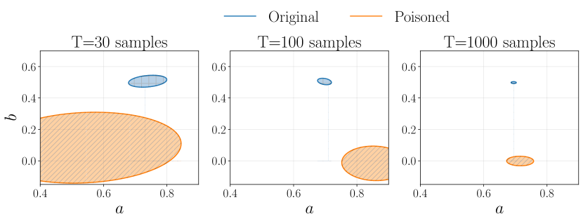
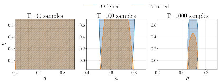
Figure 5: 95% confidence regions for $(a,b)$ and different values of the noise variance. From top to bottom: $\sigma=0.1$, $\sigma=1$, $\sigma=10$.

A.2.2 Residuals maximization attack

In example 4.9 we consider a system described by the following transfer function

$$P(s)=\frac{0.28261s+0.50666}{s^{4}-1.41833s^{3}+1.58939s^{2}-1.31608s+0.88642},$$ (14)

sampled with sampling time $\Delta T=0.05s$. From lemma 4.7 we know that $\|\tilde{R}\|_{\textnormal{F}}^{2}=Tr(W_{-}F_{T}W_{-}^{\top})+Tr(\Delta W_{-}F_{T}\Delta W_{-}^{\top})+2Tr(W_{-}F_{T}\Delta W_{-}^{\top})$, where $F_{T}=(I_{T}-\tilde{M})$ and $\tilde{M}=\begin{bmatrix}\tilde{X}_{-}\\ \tilde{U}_{-}\end{bmatrix}^{\dagger}\begin{bmatrix}\tilde{X}_{-}\\ \tilde{U}_{-}\end{bmatrix}$ is a $T\times T$ idempotent matrix. Since the first term $Tr(W_{-}F_{T}W_{-}^{\top})$ does not depend on the attack signal, for our purposes we only need to consider the latter two terms. Therefore, if the attacker wants to maximize the norm of the residuals, she simply needs to maximize $Tr(\Delta W_{-}F_{T}\Delta W_{-}^{\top})+2Tr(W_{-}F_{T}\Delta W_{-}^{\top}).$ Since the true noise sequence $W_{-}$ is not available, we approximate it using the unpoisoned residuals $R$. Similarly, in the computation of $\Delta W_{-}$ we need to know what is the true parameter $(A_{\star},B_{\star})$. As an approximation, we replace this quantity by the unpoisoned estimate $(A_{\textrm{LS}},B_{\textrm{LS}})$ . Therefore, the objective of the attacker is to maximize

$$Tr(\Delta\tilde{W}_{-}F_{T}\Delta\tilde{W}_{-}^{\top})+2Tr(RF_{T}\Delta\tilde{W}_{-}^{\top}),$$ (15)

where $\Delta\tilde{W}_{-}=\Delta X_{-}-A_{\textrm{LS}}\Delta X_{-}-B_{\textrm{LS}}\Delta U_{-}.$ This last term is clearly convex in $(\Delta X,\Delta U_{-})$, consequently maximizing it is a concave problem, where the solution is attained at the boundary of the feasible convex set, defined by the inequalities $\|\Delta X\|_{\textnormal{F}}\leq\delta\|X\|_{\textnormal{F}}$ and $\|\Delta U_{-}\|_{\textnormal{F}}\leq\delta\|U_{-}\|_{\textnormal{F}}$. Note that the total number of parameters to optimize is $Tm+(T+1)n$.

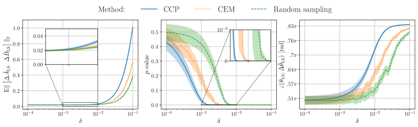
Figure 6: Untargeted attack that maximizes the MSE. On the left is shown the impact on the LS estimate; in the middle the probability under the null hypothesis of having observed $\|\tilde{R}\|_{\textnormal{F}}^{2}$; on the right the angle between the unpoisoned estimate $\theta_{\textrm{LS}}$ and the poisoned error of the estimate $\Delta\tilde{\theta}_{\textrm{LS}}$. Shadowed areas depict 95% confidence intervals over 100 runs.

To solve the problem we considered different techniques:

• Approximately exact solution: one way to solve the problem is to note that the problem can be rewritten as a difference of convex function. Therefore we can use convex-concave programming. In particular, we made use of the DCCP library [Shen et al.(2016)Shen, Diamond, Gu, and Boyd] with the MOSEK solver.

• Cross-entropy method (CEM): the cross-entropy method [De Boer et al.(2005)De Boer, Kroese, Mannor, and Rubinstein] can be used to solve the problem using samples generated from a Gaussian distribution (see also algorithm 1). We used the following parameters for algorithm 1: $\mu_{0}=0,\Sigma_{0}=I_{k},M=500,N=50,\rho=0.1,\varepsilon=1.5,\alpha=0.5$ and $\lambda=0.001$ (where $k=Tm+(T+1)n$ is the number of parameters to optimize).

• Random sampling from a Gaussian distribution: this is similar to the cross-entropy method, we sampled $100$ random points according to $\mathcal{N}(0,I_{k})$ (with $k=Tm+(T+1)n$) and re-scaled the covariance matrix to guarantee the constraints on the norm of the poisoning signals. We evaluated the MSE of each sample and chose the one that achieved the largest error.

In the simulations we considered a zero-mean Gaussian process noise with variance $\sigma_{w}=0.1$. The victim has collected $T=200$ samples using an i.i.d. control signal $u_{t}\sim\mathcal{N}(0,1)$.

Algorithm 1 Cross-Entropy Method - Gaussian Distribution

0:  Initial mean and covariance $\mu_{0}\in\mathbb{R}^{k}$ and $\Sigma_{0}\in\mathbb{R}^{k\times k}$; number of points $N$ and elite points $N_{e}$; maximum number of iterations $M$; function to evaluate $S$; smoothing factor $\alpha$; covariance threshold $\varepsilon$; regularizer $\lambda$.

1:  for $t=0,\dots,M-1$ iterations do

2:     Sampling. Generate $N$ samples $\left\{x_{1}^{(t)},\dots,x_{N}^{(t)}\right\}$ from the density $\mathcal{N}(\mu_{t},\Sigma_{t})$.

3:     Evaluation. Evaluate the performance $S(x_{i}^{(t)})$ of each sample $x_{i}^{(t)}$, and let $\mathcal{I}$ be the set of $N_{e}$ best performing samples.

4:     Update. Compute mean and covariance using the set of best performing samples

$$\hat{\mu}_{t} =\frac{1}{N_{e}}\sum_{j\in\mathcal{I}}x_{j}^{(t)},$$

$$\hat{\Sigma}_{t} =\frac{1}{N_{e}}\sum_{j\in\mathcal{I}}\left(x_{j}^{(t)}-\hat{\mu}_{t}\right)\left(x_{j}^{(t)}-\hat{\mu}_{t}\right)^{\top},$$

and update the parameters according to a smooth update

$$\mu_{t+1}=(1-\alpha)\mu_{t}+\alpha\hat{\mu}_{t},\quad\Sigma_{t+1}=(1-\alpha)\Sigma_{t}+\alpha(\hat{\Sigma}_{t}+\lambda I_{k}).$$

5:     if $\sigma_{\text{max}}(\Sigma_{t+1})\leq\varepsilon$ then

6:        Break the loop.

7:     end if

8:  end for

9:  return  Overall best solution $x_{\text{best}}$ generated by the algorithm.

A.2.3 Stealthy attack

We propose the following stealthy attack, computed by solving the following optimization problem:

$$\max_{\Delta U_{-},\Delta X} \left\lVert\begin{bmatrix}\Delta\tilde{A}_{\textrm{LS}}&\Delta\tilde{B}_{\textrm{LS}}\end{bmatrix}\right\rVert_{2}\textrm{ s.t. }g_{i}(\mathcal{D},\Delta U,\Delta X)\leq\delta_{i},\quad i=0,2,\dots,s+3,$$ (16)

where

$$g_{0} =\|\Delta X\|_{\textnormal{F}}/\|X\|_{\textnormal{F}},$$ (17)

$$g_{1} =\|\Delta U\|_{\textnormal{F}}/\|U\|_{\textnormal{F}},$$ (18)

$$g_{2} =\left|1-\|\tilde{R}\|_{\textnormal{F}}^{2}/\|R\|_{\textnormal{F}}^{2}\right|,$$ (19)

$$g_{3} =|1-Z_{\tilde{\mathcal{D}}}/Z_{\mathcal{D}}|,$$ (20)

$$g_{3+\tau} =\left|1-\|\tilde{C}_{\tau}\tilde{C}_{0}^{-1}\|_{\textnormal{F}}^{2}/\|C_{\tau}C_{0}^{-1}\|_{\textnormal{F}}^{2}\right|,\quad\tau=1,\dots,s,$$ (21)

for some $s<T-1$. As previously explained, the constraints limit the relative change of each quantity and can be made more granular, for example, by limiting the norm of the signals at each time step $t$.

Simulation settings.

We applied the attack on the following continuous-time system

$$P(s)=\frac{0.28261s+0.50666}{s^{4}-1.41833s^{3}+1.58939s^{2}-1.31608s+0.88642},$$ (22)

sampled with sampling time $\Delta T=0.05s$. The process noise is zero-mean white noise with standard deviation $\sigma_{w}=0.1$. Using $10$ different seeds, we collected $10$ different datasets $\mathcal{D}$, each with $T=500$ samples. For each datataset, 10 attacks were computed by solving the above optimization problem using sequential quadratic programming (SLSQP, a quasi-Newton approach). Out of the $10$ best attacks for each dataset, we kept only the attack that maximized the MSE. To run the simulations, we used a local stationary computer with Ubuntu 20.10, an Intel® Xeon® Silver 4110 Processor (8 cores) and 64GB of ram. On average, it took $7$ hours to compute $10$ attacks on a single dataset $\mathcal{D}$, for $\delta\in\{0.01,0.025,0.05,0.075,0.1\}$. The total simulation time took approximately $7$ days. For further details, please refer to the repository.

Results and discussion.

In fig. 7, fig. 8 and fig. 9 are shown the results of the simulation. In fig. 7 and fig. 8 are shown the statistical quantities of interest. In fig. 7 is also shown the boxplot of all leverage scores $h_{ii}$, $i=0,\dots,T-1$ ($h_{ii}$ is the $i$-th element along the diagonal of $\tilde{\Psi}_{-}^{\dagger}\tilde{\Psi}_{-}$). We note that for small values of $\delta$, the norm of the residuals $\|\tilde{R}_{t}\|_{2}$, as well as the norm of the normalized correlation matrices $\|\tilde{C}_{\tau}\tilde{C}_{0}^{-1}\|_{\textrm{F}}^{2}$, are comparable to the unpoisoned case. Interestingly, the norm of the residuals seem to be more affected by the poisoning for large values of $\delta$, which is, however, not captured by the leverage score in fig. 7.

From fig. 8 we also observe that the constraints $g_{0}$ and $g_{1}$ for large values of $\delta$ may not be very effective. In fact we note that the average norm of the residuals tend to decrease, while the number of peaks increases. This suggests that an attacker may use more granular constraints, which, however, will make the attack less effective.

However, these results also demonstrate that this attack can severely impact the LS estimate for small values of $\delta$, compared to the residuals attack presented in example 4.9. In comparison, for $\delta=0.05$ the attack impact has more than doubled, while the statistical indicators show no evidence of anomaly. In addition, for small values of $\delta$ the residuals visually do not change in a sensible way, and an analysis of the outliers, based on the concept of leverage, shows no statistical difference for any values of $\delta$ . Furthermore, for any value of $\delta$ the attack seems to impact more the estimate of $A_{\textrm{LS}}$ rather than $B_{\textrm{LS}}$, due to the presence of the constraint $g_{3}$.

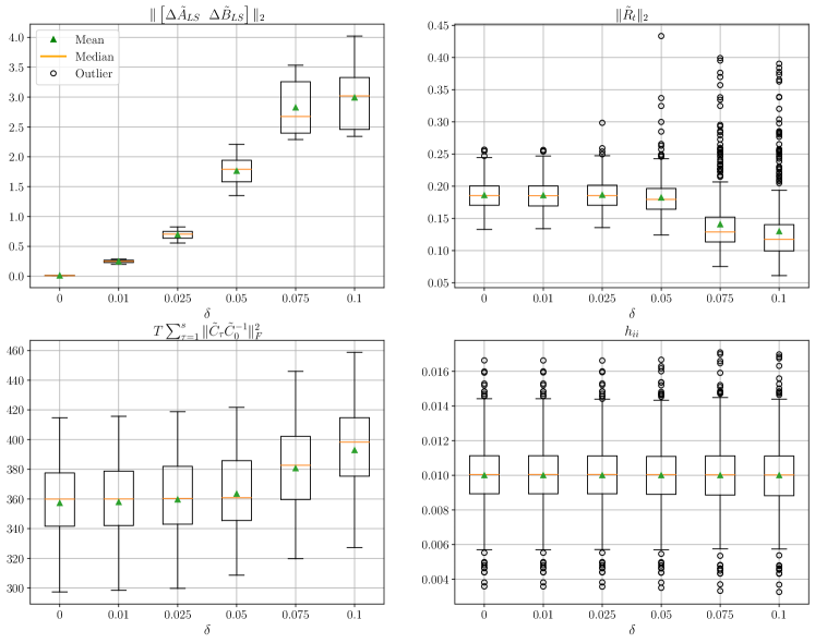
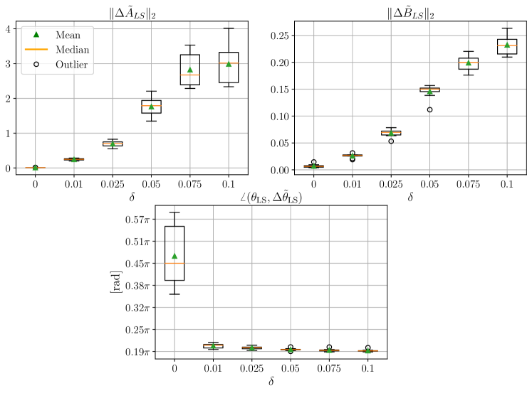
Figure 7: Statistics of the attack in eq. 9 over $10$ datasets for different values of $\delta$.

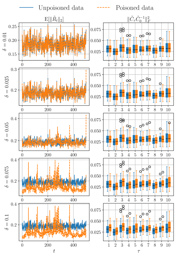
Figure 8: Residuals analysis for one of the dataset. On the left is shown the norm of the residuals when the data has been poisoned according to the attack strategy in eq. 9, for different values of $\delta$. On the right is shown $\|\tilde{C}_{\tau}\tilde{C}_{0}^{-1}\|_{\textrm{F}}^{2}$ for different values of $\tau$.

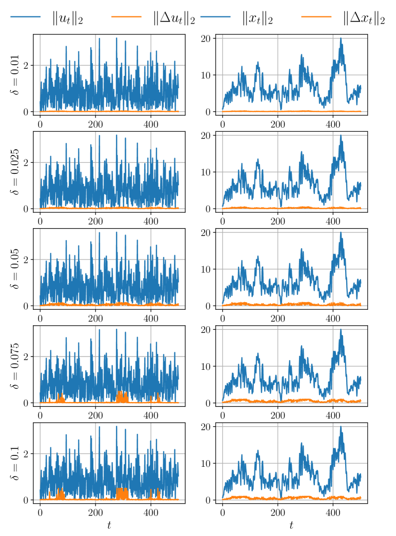
Figure 9: Comparison between the original signals $\{(u_{t},x_{t})\}_{t}$ and the poisoning signals $\{(\Delta u_{t},\Delta x_{t})\}_{t}$ for one of the dataset (computed by solving eq. 9 for different values of $\delta$).

References

• [Abbasi-Yadkori and Szepesvári(2011)] Yasin Abbasi-Yadkori and Csaba Szepesvári. Regret bounds for the adaptive control of linear quadratic systems. In Proceedings of the 24th Annual Conference on Learning Theory, pages 1–26. JMLR Workshop and Conference Proceedings, 2011.
• [Alfeld et al.(2016)Alfeld, Zhu, and Barford] Scott Alfeld, Xiaojin Zhu, and Paul Barford. Data poisoning attacks against autoregressive models. In Proceedings of the AAAI Conference on Artificial Intelligence, volume 30, 2016.
• [Barreno et al.(2006)Barreno, Nelson, Sears, Joseph, and Tygar] Marco Barreno, Blaine Nelson, Russell Sears, Anthony D Joseph, and J Doug Tygar. Can machine learning be secure? In Proceedings of the 2006 ACM Symposium on Information, computer and communications security, pages 16–25, 2006.
• [Barreno et al.(2010)Barreno, Nelson, Joseph, and Tygar] Marco Barreno, Blaine Nelson, Anthony D Joseph, and J Doug Tygar. The security of machine learning. Machine Learning, 81(2):121–148, 2010.
• [Bhatia et al.(2015)Bhatia, Jain, and Kar] Kush Bhatia, Prateek Jain, and Purushottam Kar. Robust regression via hard thresholding. Advances in neural information processing systems, 28, 2015.
• [Bhatia et al.(2017)Bhatia, Jain, Kamalaruban, and Kar] Kush Bhatia, Prateek Jain, Parameswaran Kamalaruban, and Purushottam Kar. Consistent robust regression. Advances in Neural Information Processing Systems, 30, 2017.
• [Biggio et al.(2012)Biggio, Nelson, and Laskov] Battista Biggio, Blaine Nelson, and Pavel Laskov. Poisoning attacks against support vector machines. In Proceedings of the 29th International Coference on International Conference on Machine Learning, pages 1467–1474, 2012.
• [Bittanti et al.(1992)Bittanti, Campi, and Lorito] Sergio Bittanti, Marco Campi, and Fabrizio Lorito. Effective identification algorithms for adaptive control. International journal of adaptive control and signal processing, 6(3):221–235, 1992.
• [Box et al.(2015)Box, Jenkins, Reinsel, and Ljung] George EP Box, Gwilym M Jenkins, Gregory C Reinsel, and Greta M Ljung. Time series analysis: forecasting and control. John Wiley & Sons, 2015.
• [Campi et al.(2002)Campi, Lecchini, and Savaresi] Marco C Campi, Andrea Lecchini, and Sergio M Savaresi. Virtual reference feedback tuning: a direct method for the design of feedback controllers. Automatica, 38(8):1337–1346, 2002.
• [Chekan and Langbort(2020)] Jafar Abbaszadeh Chekan and Cedric Langbort. Regret bounds for lq adaptive control under database attacks (extended version). arXiv preprint arXiv:2004.00241, 2020.
• [Coulson et al.(2019)Coulson, Lygeros, and Dörfler] Jeremy Coulson, John Lygeros, and Florian Dörfler. Data-enabled predictive control: In the shallows of the deepc. In 2019 18th European Control Conference (ECC), pages 307–312. IEEE, 2019.
• [De Boer et al.(2005)De Boer, Kroese, Mannor, and Rubinstein] Pieter-Tjerk De Boer, Dirk P Kroese, Shie Mannor, and Reuven Y Rubinstein. A tutorial on the cross-entropy method. Annals of operations research, 134(1):19–67, 2005.
• [De Persis and Tesi(2019)] Claudio De Persis and Pietro Tesi. Formulas for data-driven control: Stabilization, optimality, and robustness. IEEE Transactions on Automatic Control, 65(3):909–924, 2019.
• [Drouiche(2000)] K Drouiche. A new test for whiteness. IEEE transactions on signal processing, 48(7):1864–1871, 2000.
• [Feng and Lavaei(2021)] Han Feng and Javad Lavaei. Learning of dynamical systems under adversarial attacks. In 2021 60th IEEE Conference on Decision and Control (CDC), pages 3010–3017. IEEE, 2021.
• [Hjalmarsson(2002)] Håkan Hjalmarsson. Iterative feedback tuning—an overview. International journal of adaptive control and signal processing, 16(5):373–395, 2002.
• [Hosking(1980)] Jonathan RM Hosking. The multivariate portmanteau statistic. Journal of the American Statistical Association, 75(371):602–608, 1980.
• [Jagielski et al.(2018)Jagielski, Oprea, Biggio, Liu, Nita-Rotaru, and Li] Matthew Jagielski, Alina Oprea, Battista Biggio, Chang Liu, Cristina Nita-Rotaru, and Bo Li. Manipulating machine learning: Poisoning attacks and countermeasures for regression learning. In 2018 IEEE Symposium on Security and Privacy (SP), pages 19–35. IEEE, 2018.
• [Kannan and Manoj(2015)] K Senthamarai Kannan and K Manoj. Outlier detection in multivariate data. Applied Mathematical Sciences, 47(9):2317–2324, 2015.
• [Karimi et al.(2004)Karimi, Mišković, and Bonvin] A Karimi, L Mišković, and D Bonvin. Iterative correlation-based controller tuning. International journal of adaptive control and signal processing, 18(8):645–664, 2004.
• [Kleinbaum et al.(2013)Kleinbaum, Kupper, Nizam, and Rosenberg] David G Kleinbaum, Lawrence L Kupper, Azhar Nizam, and Eli S Rosenberg. Applied regression analysis and other multivariable methods. Cengage Learning, 2013.
• [Kloft and Laskov(2010)] Marius Kloft and Pavel Laskov. Online anomaly detection under adversarial impact. In Proceedings of the thirteenth international conference on artificial intelligence and statistics, pages 405–412. JMLR Workshop and Conference Proceedings, 2010.
• [Koch et al.(2020)Koch, Berberich, and Allgöwer] Anne Koch, Julian Berberich, and Frank Allgöwer. Verifying dissipativity properties from noise-corrupted input-state data. In 2020 59th IEEE Conference on Decision and Control (CDC), pages 616–621. IEEE, 2020.
• [Liu et al.(2017)Liu, Ma, Aafer, Lee, Zhai, Wang, and Zhang] Yingqi Liu, Shiqing Ma, Yousra Aafer, Wen-Chuan Lee, Juan Zhai, Weihang Wang, and Xiangyu Zhang. Trojaning attack on neural networks. 2017.
• [Ljung(1998)] Lennart Ljung. System identification. In Signal analysis and prediction, pages 163–173. Springer, 1998.
• [Massey Jr(1951)] Frank J Massey Jr. The kolmogorov-smirnov test for goodness of fit. Journal of the American statistical Association, 46(253):68–78, 1951.
• [Nelson(1998)] Lloyd S Nelson. The anderson-darling test for normality. Journal of Quality Technology, 30(3):298, 1998.
• [Nguyen and Tran(2013)] Nam H Nguyen and Trac D Tran. Exact recoverability from dense corrupted observations via $\ell_{1}$-minimization. IEEE transactions on information theory, 59(4):2017–2035, 2013.
• [Rubinstein et al.(2009)Rubinstein, Nelson, Huang, Joseph, Lau, Rao, Taft, and Tygar] Benjamin IP Rubinstein, Blaine Nelson, Ling Huang, Anthony D Joseph, Shing-hon Lau, Satish Rao, Nina Taft, and J Doug Tygar. Antidote: understanding and defending against poisoning of anomaly detectors. In Proceedings of the 9th ACM SIGCOMM Conference on Internet Measurement, pages 1–14, 2009.
• [Russo and Proutiere(2021)] Alessio Russo and Alexandre Proutiere. Poisoning attacks against data-driven control methods. In 2021 American Control Conference (ACC), pages 3234–3241. IEEE, 2021.
• [Russo et al.(2021)Russo, Molinari, and Proutiere] Alessio Russo, Marco Molinari, and Alexandre Proutiere. Data-driven control and data-poisoning attacks in buildings: the kth live-in lab case study. In 2021 29th Mediterranean Conference on Control and Automation (MED), pages 53–58. IEEE, 2021.
• [Shafahi et al.(2018)Shafahi, Huang, Najibi, Suciu, Studer, Dumitras, and Goldstein] Ali Shafahi, W Ronny Huang, Mahyar Najibi, Octavian Suciu, Christoph Studer, Tudor Dumitras, and Tom Goldstein. Poison frogs! targeted clean-label poisoning attacks on neural networks. Advances in neural information processing systems, 31, 2018.
• [Shen et al.(2016)Shen, Diamond, Gu, and Boyd] Xinyue Shen, Steven Diamond, Yuantao Gu, and Stephen Boyd. Disciplined convex-concave programming. In 2016 IEEE 55th Conference on Decision and Control (CDC), pages 1009–1014. IEEE, 2016.
• [Showkatbakhsh et al.(2016)Showkatbakhsh, Tabuada, and Diggavi] Mehrdad Showkatbakhsh, Paulo Tabuada, and Suhas Diggavi. Secure system identification. In 2016 54th Annual Allerton Conference on Communication, Control, and Computing (Allerton), pages 1137–1141. IEEE, 2016.
• [Tian et al.(2022)Tian, Cui, Liang, and Yu] Zhiyi Tian, Lei Cui, Jie Liang, and Shui Yu. A comprehensive survey on poisoning attacks and countermeasures in machine learning. ACM Computing Surveys (CSUR), 2022.
• [Willems et al.(2005)Willems, Rapisarda, Markovsky, and De Moor] Jan C Willems, Paolo Rapisarda, Ivan Markovsky, and Bart LM De Moor. A note on persistency of excitation. Systems & Control Letters, 54(4):325–329, 2005.
• [Xiao et al.(2015)Xiao, Biggio, Brown, Fumera, Eckert, and Roli] Huang Xiao, Battista Biggio, Gavin Brown, Giorgio Fumera, Claudia Eckert, and Fabio Roli. Is feature selection secure against training data poisoning? In international conference on machine learning, pages 1689–1698. PMLR, 2015.
• [Yu et al.(2022)Yu, Zhao, Chinchali, and Topcu] Yue Yu, Ruihan Zhao, Sandeep Chinchali, and Ufuk Topcu. Poisoning attacks against data-driven predictive control, 2022. URL https://arxiv.org/abs/2209.09108.
• [Zhang et al.(2020)Zhang, Zhu, and Lessard] Xuezhou Zhang, Xiaojin Zhu, and Laurent Lessard. Online data poisoning attacks. In Learning for Dynamics and Control, pages 201–210. PMLR, 2020.