Adapting to noise distribution shifts in flow-based gravitational-wave inference

Abstract

Deep learning techniques for gravitational-wave parameter estimation have emerged as a fast alternative to standard samplers—producing results of comparable accuracy. These approaches (e.g., Dingo) enable amortized inference by training a normalizing flow to represent the Bayesian posterior conditional on observed data. By conditioning also on the noise power spectral density (PSD) they can even account for changing detector characteristics. However, training such networks requires knowing in advance the distribution of PSDs expected to be observed, and therefore can only take place once all data to be analyzed have been gathered. Here, we develop a probabilistic model to forecast future PSDs, greatly increasing the temporal scope of Dingo networks. Using PSDs from the second LIGO-Virgo observing run (O2)—plus just a single PSD from the beginning of the third (O3)—we show that we can train a Dingo network to perform accurate inference throughout O3 (on 37 real events). We therefore expect this approach to be a key component to enable the use of deep learning techniques for low-latency analyses of gravitational waves.

I Introduction

Detector noise plays a crucial role in interpreting observations of gravitational waves (GWs). In its simplest form, noise is assumed to be additive, and stationary and Gaussian. This means that it is characterized in frequency domain by its power spectral density (PSD) $S_{\text{n}}(f)$. The GW likelihood for parameters $\theta$ is then the probability that after a proposed signal $h(\theta)$ is subtracted from data $d$, the residual is noise satisfying these assumptions, i.e.,

$$p(d|\theta,S_{\text{n}})\propto\exp\left(-\frac{1}{2}(d-h(\theta)|d-h(\theta))_{S_{\text{n}}}\right),$$ (1)

where $(\cdot|\cdot)$ is the noise-weighted inner-product,

$$(a|b)_{S_{\text{n}}}=4\sum_{I}\Re\int_{f_{\text{min}}}^{f_{\text{max}}}\frac{\hat{a}_{I}^{\ast}(f)\hat{b}_{I}(f)}{S_{\text{n},I}(f)}df,$$ (2)

and the sum runs over interferometers $I$.

Although the LIGO [1], Virgo [2] and KAGRA [3, 4, 5] detectors are mostly stable during an observing run, the noise spectrum does vary over time and across detectors. Moreover, between observing runs, detectors are upgraded, resulting in reduced noise levels and increased sensitivity. The particular PSDs at the time of an event must therefore be estimated and taken into account when performing inference. Estimation of a PSD is typically carried out using either data adjacent to an event (off-source, Welch method [6]) or by jointly modeling the signal and noise from the on-source data (e.g., BayesWave [7, 8]). The PSD is then inserted into the likelihood and samples are drawn from the posterior $p(\theta|d,S_{\text{n}})$ using Markov chain Monte Carlo [9] or nested sampling methods [10, 11, 12].

An emerging alternative to classical likelihood-based inference is simulation-based inference using probabilistic deep learning [13, 14, 15, 16, 17, 18, 19, 20, 21, 22]. Technologies such as normalizing flows enable neural networks to describe complex conditional probability distributions. A conditional density estimator $q(\theta|d)$ can be trained using simulated data to approximate $p(\theta|d)$ such that once a detection is made, samples can be drawn in seconds. To incorporate varying noise PSDs into these methods, the estimate of $S_{\text{n}}$ is provided as additional context to the network, i.e. $q(\theta|d,S_{\text{n}})$. During training, random PSDs are drawn from an empirical distribution $p(S_{\text{n}})$ estimated from signal-free data during an observing run. Simulated data are then constructed based on these PSDs, and the PSD is provided as context. At inference time, the network is effectively “tuned” to the interferometers at the time of detection. This approach (called Dingo [19]) fully amortizes training costs across all detections within an observing run, and has been shown to produce results nearly indistinguishable from classical samplers.

The approach described requires access to the empirical distribution $p(S_{\text{n}})$ of PSDs during an observing run. This makes it unsuitable for online parameter estimation (e.g., to provide alerts to electromagnetic telescopes) since the distribution $p(S_{\text{n}})$ covering future observations is unavailable at the time of network training. Thus, a network trained with an empiric PSD distribution can only be used for a limited time—once the PSDs change too much, the measured data become out-of-distribution (OOD). Such a disagreement between training and inference distributions can lead to inaccurate results (Fig. 1). Here, we address this problem and provide a solution for training Dingo models robustly to better adapt to shifting distributions.

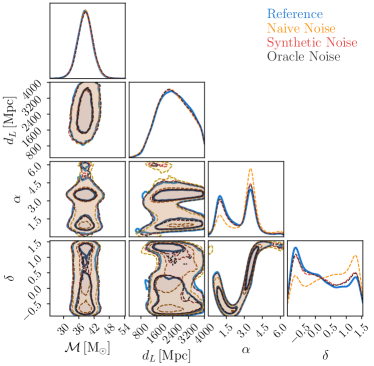
Figure 1: Posterior for GW200208_130117. Results from Dingo models trained only with empirically estimated detector-noise PSDs from the beginning of an observing run (orange) may deviate visibly from the reference (blue, obtained using importance sampling [23]). Dingo models trained with our proposed synthetic PSD model (red) achieve much more accurate results, on par with using PSDs estimated throughout the entire observing run (black). Our PSD model therefore enables Dingo to adapt to unseen drifts of the PSDs without retraining.

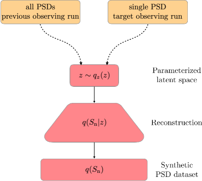
Figure 2: Overview of the PSD generation pipeline. The PSDs from the previous observing run and a single PSD from the target observing run are used for fitting the latent distribution $q_{z}(z)$, as indicated by the dashed arrows. We can then generate synthetic PSDs by first sampling latent variables in $z\sim q_{z}(z)$. These are then reconstructed back to frequency space via $q(S_{\text{n}}|z)$, obtaining a synthetic PSD distribution $q(S_{\text{n}})$.

Our approach is based on the key property that Dingo models $q(\theta|d,S_{\text{n}})$ estimate a distribution conditional on (as opposed to marginalized over) the PSD $S_{\text{n}}$. We are therefore not restricted to using (an approximation to) the real distribution $p(S_{\text{n}})$ of PSDs; instead, we can use a synthetic distribution $q(S_{\text{n}})$ whose support contains that of $p(S_{\text{n}})$. In other words, if $\operatorname{supp}p(S_{\text{n}})\subseteq\operatorname{supp}q(S_{\text{n}})$, then the Dingo model trained with $q(S_{\text{n}})$ can be used for the entire observing run.

In this work, we develop a parameterized latent variable model for $q(S_{\text{n}})$, which we fit to PSDs from a previous observing run. It is then straightforward to modify this distribution of PSDs via operations on the latent space. In particular, we use a one-shot observation from an upgraded detector to shift the latent space distribution coarsely to the expected noise level. Further, we broaden the spread of PSDs by blurring the latent space distribution. Our model $q(S_{\text{n}})$ thereby represents a broad distribution over PSDs, which is capable of capturing variations throughout an observing run.

We evaluate our approach on the third LIGO-Virgo-KAGRA (LVK) observing run (O3) by analyzing 390 simulated and 37 real GW events [24]. We train Dingo with our PSD model and consistently find similar performance to Dingo trained with real O3 PSDs. Since our PSD model only uses O2 data and a single PSD from the beginning of O3, this demonstrates that our approach is indeed capable of preparing Dingo for unseen PSD changes.

II Methods

In probabilistic modeling, a latent variable model [25, 26, 27] enables efficient sampling of new data given an empirical distribution. We define a latent variable model for the PSDs, as

$$q(S_{\text{n}})=\int q(S_{\text{n}}|z)q_{z}(z)dz.$$ (3)

We use a fixed parameterization for $q(S_{\text{n}}|z)$ to integrate knowledge about the data generating process into the model. PSD data can then be fitted via the distribution $q_{z}(z)$ over the latent variables. This provides an interpretable framework, enabling systematic interventions on the PSD distribution. Synthetic PSDs can then be generated by sampling $z\sim q_{z}(z)$ and reconstructing $z$ back to frequency space via $q(S_{\text{n}}|z)$. This pipeline is visualized in Fig. 2; next we explain the individual components in detail.

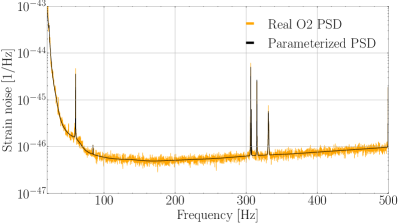
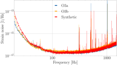
Figure 3: Upper panel: Comparison of a real O2 PSD and its representation under the latent variable model. Since $l=400$ is sufficiently large, we can accurately model spectral lines that are close together (at around 300Hz). Lower panel: Comparison of a synthetically sampled PSD and two real PSDs from O3a and O3b. By shifting the broad-band noise level (II.3), we match the overall scale of O3 PSDs. By broadening the distribution, we ensure that PSDs from both O3a and O3b are covered.

II.1 Parametrization of $q(S_{\text{n}}|z)$

We aim to design a model $q(S_{\text{n}})$ with sufficient expressiveness to capture every realistic PSD. On the other hand, the latent space should be low dimensional and maximally disentangled, such that the distribution $q_{z}(z)$ partially factorizes. In particular, the latent features $z$ should model those PSD characteristics that are likely to change over time. This increases the data efficiency and robustness of our model under interventions. These requirements inform our design of $q(S_{\text{n}}|z)$.

We leverage domain knowledge to parameterize the latent feature space explicitly. Each PSD is represented by a $n$-dimensional vector $S_{\text{n}}\in\mathbb{R}^{n}$ for uniformly distributed frequency bins $f_{1},\ldots,f_{n}$ in the range $[f_{\text{min}},f_{\text{max}}]$. According to [28], $S_{\text{n}}$ can be decomposed into two main components, the smooth broad-band noise $b\in\mathbb{R}^{n}$ and a sum of high-power spectral lines $\sum_{i}s_{i}\in\mathbb{R}^{n}$. Improvements to the detectors are intended to reduce the impact of the broad-band noise, making it likely to change over time. The position and shape of the spectral lines may vary on much shorter time-scales. We thus model these components independently. We further assume independent additive Gaussian noise with constant variance $\sigma^{2}$ in each frequency bin.

With these assumptions, our model reads

$$q(S_{\text{n}}|z)=\mathcal{N}\left(b+\sum_{i=1}^{l}s_{i},\sigma^{2}I_{n}\right).$$ (4)

In latent space, the broad-band noise is represented by $k$ values $y_{1},\ldots,y_{k}\in\mathbb{R}_{+}$ on fixed log-spaced frequency nodes $x_{1},\ldots,x_{k}$. The logarithmic distribution accounts for larger fluctuations of the broad-band noise in lower frequency regions. $b$ is then obtained from its latent representation via cubic spline interpolation between the nodes.

Each spectral line $s_{i}$ is represented by parameters $f_{0i},A_{i},Q_{i}$, denoting the center, height, and width of a truncated Cauchy distribution, respectively, i.e.

$$s_{i}[f_{0i},A_{i},Q_{i}](f)=\frac{z(f,f_{0i})A_{i}f_{0i}^{4}}{(f_{0i}f)^{2}+(Q_{i}(f_{0i}^{2}-f^{2}))^{2}},$$ (5)

with

$$z(f,f_{0i})=\begin{cases}1,&\text{if }|f-f_{0i}|\leq\delta,\\ \exp(-\frac{|f-f_{0i}|}{\delta}),&\text{otherwise},\end{cases}$$ (6)

similarly to [28]. To efficiently treat a varying number of spectral lines per PSD, we segment the frequency range into $l$ equally-wide intervals and model a single spectral line within each. Absence of a spectral line is modeled with $A_{i}\approx 0$. We do not find that restricting to one line per interval hinders Dingo performance in practice, provided the number of intervals is sufficiently large; see Fig. 3 (upper panel). In our experiments, we used $k=30$, and $l=400$ over a frequency range of $[f_{\text{min}},f_{\text{max}}]=[20,2048]\leavevmode\nobreak\ \text{Hz}$. If desired, the model could be extended to use overlapping intervals. In this case, each spectral distribution would no longer be independent, but rather conditional on the parameters of the preceding frequency interval.

We found that $\sigma^{2}$ does not vary significantly between different PSDs. We therefore use a fixed value for $\sigma^{2}$ (estimated from the variance of the observed broad-band noise), and do not consider it as part of our latent space. Summarizing, our mapping from the latent space to frequency space reads

$$z=\begin{pmatrix}y_{1},\ldots,y_{k},\\ f_{01},A_{1},Q_{1},\\ \vdots\\ f_{0l},A_{l},Q_{l}\end{pmatrix}\mapsto S_{\text{n}}.$$ (7)

The dimensionality of our latent space is $d=k+3l$.

II.2 Fitting the latent distribution $q_{z}(z)$

We fit $q_{z}(z)$ based on an empirical distribution of PSDs estimated from detector data. We estimate this collection of PSDs using Welch’s method applied to signal-free data stretches during the previous observing run. We then project these onto the latent space using maximum likelihood estimation and obtain $q_{z}(z)$ as the product of Gaussian kernel density estimates (KDEs) of these projections. This gives a tractable approximation to the true latent distribution. Importantly, having an analytic KDE provides flexibility to widen $q_{z}(z)$ by increasing the KDE bandwidth.

We perform the maximum likelihood projection onto the latent space in two steps. We first estimate the spline parameters $y_{1},\ldots,y_{k}$ for the broad-band noise as the sample mean of the PSD in the vicinity of the corresponding $x_{i}$. Since the broad-band noise should not model the spectral lines, we apply a filter before this step. Once the broad-band noise is fitted, we subtract it from the PSD to fit the spectral lines. Specifically, we obtain $(f_{0i},A_{i},Q_{i})$ by solving the least-squares problem

$$\begin{split}(f_{0i},A_{i},Q_{i})&=\operatorname*{arg\,min}_{(\tilde{f},\tilde{A},\tilde{Q})}\sigma^{-2}rr^{\top}\\ r=r(f,A,Q)&=S_{\text{n}}-(b+s_{i}(f,A,Q)),\end{split}$$ (8)

over each interval $i$. Together, these two steps correspond to a maximum-likelihood estimate of $z$ for (4) with fixed $\sigma^{2}$. On eight CPU cores, it takes less than a minute to obtain the latent maximum likelihood estimate $z_{\text{MLE}}$ for each PSD, and this procedure is straightforwardly parallelizable. Indeed, this fast calculation (compared to $\approx 1$ hour for BayesLine) is one reason for choosing this simpler approach when building our PSD model.

Having computed $z_{\text{MLE}}$ for each PSD from the empiric distribution, we next use KDEs to obtain $q_{z}(z)$. We use a separate KDE for each ”independent” noise source, and then combine them multiplicatively. For the broad-band noise, we partition the frequency range into three intervals according to the most dominant noise source: $\mathcal{F}_{1}=[f_{\text{min}},30\leavevmode\nobreak\ \text{Hz}]$ for seismic noise, $\mathcal{F}_{2}=[30\leavevmode\nobreak\ \text{Hz},100\leavevmode\nobreak\ \text{Hz}]$ for thermal noise and $\mathcal{F}_{3}=[100\leavevmode\nobreak\ \text{Hz},f_{\text{max}}]$ for shot noise [28]. Since these noise sources should be largely independent of each other, we use individual KDEs for each subset $\{y_{i}\ |\ x_{i}\in\mathcal{F}_{j}\}$. These subsets do not overlap, so the reconstructed spline naturally agrees on the boundary between intervals $\mathcal{F}_{i}$. Similarly, the spectral lines are modeled independently, so we use a separate KDE for each set of parameters $(f_{0i},A_{i},Q_{i})$. The latent distribution is then given as the product of the $3+l$ individual KDEs.

The independence assumption made above, and the corresponding partial factorization of $q_{z}(z)$ into $3+l$ independent distributions, serves two purposes. First, it provides broader coverage of the latent space compared to an unfactorized KDE. Second, it decorrelates factors of variation that are independent so that trained networks do not learn to expect spurious correlations that exist in the empirical PSDs. Both of these effects ensure that trained networks are generally more robust with respect to changes in the PSD so that they can adapt to unseen data.

II.3 Interventions in latent space

The latent space is much lower dimensional than the raw PSD space and has features that correspond to the main components comprising a PSD. By intervening in this space (i.e., changing the PSD distribution at the level of the latent space) we can therefore naturally adapt the PSD distribution to changing detector noise characteristics. We perform two such types of interventions: (1) we shift the broad-band noise to account for improved detector sensitivity, and (2) we broaden the distribution to account for uncertainty in the estimated broad-band shift and other unmodeled detector changes.

For (1), we rescale the latent distribution over $y_{1},\ldots,y_{k}$ according to an estimated PSD from early in the target run. Given a single PSD $S_{\text{n}}^{\text{target}}$ from the target run, we shift the distribution over $y_{i}$ so that its mean corresponds to the target PSD, i.e.,

$$y_{i}\mapsto y_{i}-\mathbb{E}[y_{i}]+y_{i}^{\text{target}}.$$ (9)

Here, $y_{i}^{\text{target}}$ refers to the latent features corresponding to $S_{n}^{\text{target}}$. The resulting distribution corresponds to variations in all latent variables inferred from past data, but with broad-band noise level shifted to that of the target observing run. Note that this works even when $S_{\text{n}}^{\text{target}}$ is not close to the mean of the target run, as long as the difference is small compared to the variance of the estimated distribution. In Fig. 3, we illustrate how this intervention on the latent space ensures that synthetically generated PSDs match the broad-band noise level of O3 PSDs (lower panel), despite the difference in scale between O2 and O3.

The broadening (2) is controlled by the KDE bandwidth parameter, and it improves the robustness of Dingo networks trained with the synthetic noise distribution. A larger bandwidth parameter can compensate for more significant shifts in the PSD distribution, although it may require higher learning capacity.

III Results

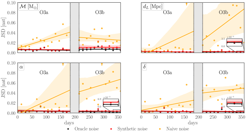
Figure 4: JSDs between Dingo and reference samples. Injections use noise PSDs estimated at various times throughout O3 (indicated on horizontal axis). Results are averaged over injections with five random sets of source parameters (fixed for all PSDs). Day 0 marks the beginning of O3a. The gap indicates the period when detectors were offline between O3a and O3b.

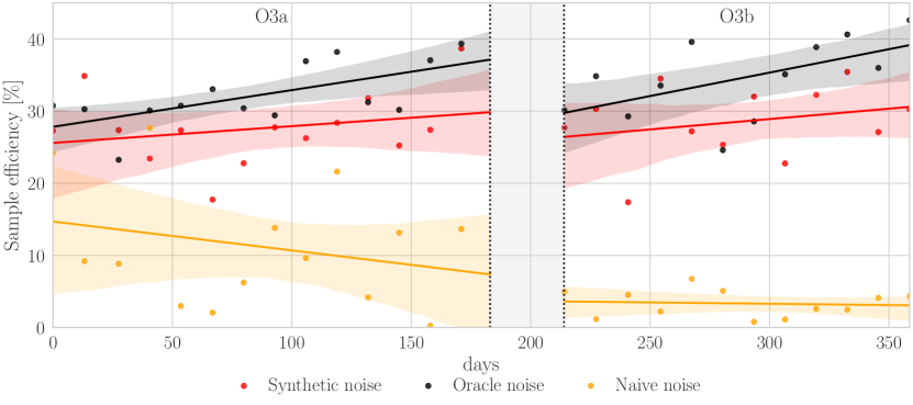
Figure 5: Importance sampling efficiency $\epsilon$ for Dingo models. Injections use noise PSDs estimated at various times throughout O3 (indicated on horizontal axis). Results are averaged over injections with five random sets of source parameters (fixed for all PSDs). Day 0 marks the beginning of O3a. The gap indicates the period when detectors were offline between O3a and O3b.

We prepare Dingo networks with the settings from [19]. In particular, we use the waveform model IMRPhenomPv2 [29, 30, 31] with frequency-domain data in the range $[20,1024]$ Hz, $\Delta f=0.125$ Hz, and a uniform distance prior of $[0.1,2]$ Gpc. We train three networks, each with a different noise PSD dataset: (1) the Oracle dataset consists of PSDs estimated from real O3a and O3b detector noise ($\sim$5,000 PSDs per detector); (2) the Synthetic dataset is sampled with our proposed method, using only O2 data and a single PSD from the start of O3 (50,000 PSDs per detector); and (3) the Naive baseline dataset consists of real PSDs from the first four days of O3a (100 PSDs per detector). The Oracle dataset encompasses the real PSDs that Dingo encounters at inference time, so this should be an upper bound for the performance of our method. On the other hand, the Naive dataset is based only on data available at the beginning of O3, so to be useful our method should significantly outperform this baseline.

We evaluate the three Dingo networks on simulated and real strain data. To assess performance, we compare against reference posteriors. Since we analyze more than 400 events, generating these using stochastic samplers is not feasible. Instead, we generate reference posteriors by importance-weighting the Dingo results produced with the Oracle PSD dataset, which provides verified inference results at low computational cost (Dingo-IS) [23]. To save computational time, we further use phase marginalization when calculating the likelihoods [32, 9, 33]. We note that with precessing waveforms this is only an approximation, but for IMRPhenomPv2 the error introduced is small. See [23] for an alternative approach to generate the phase in the presence of higher modes.

III.1 Simulated data

We first evaluate inference results when solely the PSD is varied in the strain data. To this end, we sample gravitational-wave parameters from the prior and inject the signal into identical noise realizations that are scaled with different PSDs. Specifically, we choose 26 real PSDs from O3, evenly spaced in time over the course of one year. The injection strains are then analyzed using each of the three Dingo networks.

Fig. 4 shows the mean Jensen-Shannon divergence (JSD) [34] between Dingo and Dingo-IS posteriors for chirp mass ($\mathcal{M}$), luminosity distance ($d_{\text{L}}$) and sky position ($\alpha,\delta$). These parameters have been found to be most significantly impacted by conditioning the network on an incorrect PSD at inference time [19]. (We find a similar trend for training with incomplete PSD information.) Results for all 15 parameters are provided in the appendix, showing a similar qualitative behavior to the parameters reported here.

At the beginning of the observing run, we observe similar accuracy for all three networks. This is not surprising, as the PSDs are still captured by the Naive dataset at this point. However, as PSDs drift away from their initial distribution, the performance of the Naive baseline decreases substantially, with JSDs increasing by one to two orders-of-magnitude. The effect is particularly striking at the transition from O3a to O3b. This demonstrates that the Naive baseline indeed fails to generalize well to unseen PSDs. The Oracle network on the other hand shows excellent performance throughout the entire duration of O3, with JSDs around $2\cdot 10^{-3}$ nat. This is also expected, since the Oracle network has access to PSDs from the entire duration of O3 during training.

Finally, with the Synthetic PSD dataset, Dingo accuracy approaches that of the Oracle network—even for PSDs recorded almost a year after the PSD used to recalibrate the Synthetic dataset (zoomed-in parts in Fig. 4). It far outperforms the Naive baseline, demonstrating that with our proposed method, Dingo can indeed be trained to generalize to unseen PSDs, with at most a small decrease in accuracy.

In the same experiment, we study the sample efficiency $\epsilon$ when using the inferred Dingo posterior as a proposal distribution for importance sampling [23] (Fig. 5). Small values of $\epsilon$ have been found to flag failure cases of the inference network, e.g., caused by out-of-distribution data, establishing it as another quality measure of the Dingo posteriors. For the Naive baseline, $\epsilon$ decreases with time and plummets after the transition from O3a to O3b. In contrast, the Oracle and Synthetic networks provide a consistently high sample efficiency of $\epsilon\approx 30\%$. As a performance metric, $\epsilon$ is sensitive to deviations in full parameter space, including high-dimensional correlations. Fig. 5 thus confirms the trend observed for the JSDs, and demonstrates that the Synthetic PSD dataset can be used to ensure a high efficiency of Dingo-IS throughout an observing run.

	Noise datasets
Event	Oracle	Synthetic	Naive
GW190408_181802	$2.1$	$4.0$	$3.1$
GW190413_052954	$0.2$	$0.5$	$0.4$
GW190413_134308	$0.9$	$0.6$	$2.0$
GW190421_213856	$0.3$	$0.4$	$0.5$
GW190503_185404	$1.1$	$2.7$	$1.6$
GW190513_205428	$2.1$	$3.7$	$2.9$
GW190514_065416	$0.5$	$0.5$	$0.7$
GW190517_055101	$21.3$	$25.4$	$14.2$
GW190519_153544	$1.2$	$1.4$	$1.2$
GW190521_074359	$1.4$	$2.4$	$2.7$
GW190527_092055	$5.5$	$2.1$	$1.4$
GW190602_175927	$1.9$	$1.9$	$3.3$
GW190701_203306	$1.2$	$1.4$	$1.4$
GW190719_215514	$0.7$	$0.3$	$0.4$
GW190727_060333	$0.3$	$0.6$	$0.6$
GW190731_140936	$0.3$	$0.4$	$1.1$
GW190803_022701	$0.6$	$0.3$	$1.4$
GW190805_211137	$0.3$	$0.4$	$1.1$
GW190828_063405	$0.7$	$2.1$	$2.6$

	Noise datasets
Event	Oracle	Synthetic	Naive
GW190909_114149	$0.4$	$0.5$	$0.9$
GW190915_235702	$0.8$	$0.7$	$1.4$
GW190926_050336	$1.7$	$1.8$	$1.8$
O3b $\downarrow$
GW191127_050227	$3.5$	$1.7$	$3.2$
GW191204_110529	$3.1$	$4.4$	$6.1$
GW191215_223052	$0.8$	$1.1$	$2.8$
GW191222_033537	$0.4$	$0.5$	$1.4$
GW191230_180458	$0.3$	$0.4$	$0.7$
GW200128_022011	$0.6$	$1.0$	$2.9$
GW200129_065458	$2.6$	$1.6$	$5.3$
GW200208_130117	$0.5$	$0.6$	$5.5$
GW200208_222617	$2.3$	$2.3$	$3.1$
GW200209_085452	$1.3$	$1.8$	$2.2$
GW200216_220804	$0.4$	$0.9$	$3.5$
GW200219_094415	$0.8$	$1.0$	$4.0$
GW200220_124850	$0.2$	$0.3$	$0.7$
GW200224_222234	$0.7$	$1.4$	$14.5$
GW200311_115853	$1.6$	$2.6$	$10.2$

Table 1: 37 binary black hole events from GWTC-2 and GWTC-3 analyzed with Dingo trained with three different PSD datasets. We report the JSD (in units of $10^{-3}$ nat) between Dingo and reference posteriors, averaged over all inferred source parameters.

	Noise datasets
Event	Oracle	Synthetic	Naive
GW190408_181802	$28.5$	$19.4$	$17.3$
GW190413_052954	$44.6$	$45.0$	$41.9$
GW190413_134308	$41.0$	$49.3$	$43.6$
GW190421_213856	$51.1$	$46.2$	$44.7$
GW190503_185404	$46.9$	$40.4$	$35.4$
GW190513_205428	$28.4$	$28.0$	$16.0$
GW190514_065416	$34.5$	$37.5$	$37.3$
GW190517_055101	$20.5$	$13.6$	$23.0$
GW190519_153544	$41.0$	$41.7$	$25.3$
GW190521_074359	$30.9$	$27.8$	$18.9$
GW190527_092055	$25.8$	$33.6$	$28.6$
GW190602_175927	$41.7$	$46.0$	$38.8$
GW190701_203306	$27.5$	$33.5$	$26.4$
GW190719_215514	$24.3$	$22.9$	$23.4$
GW190727_060333	$42.7$	$48.7$	$31.1$
GW190731_140936	$46.5$	$47.7$	$33.9$
GW190803_022701	$51.8$	$45.5$	$48.0$
GW190805_211137	$50.1$	$51.8$	$39.2$
GW190828_063405	$50.8$	$35.4$	$34.2$

	Noise datasets
Event	Oracle	Synthetic	Naive
GW190909_114149	$32.9$	$17.6$	$22.5$
GW190915_235702	$49.3$	$48.7$	$45.1$
GW190926_050336	$30.8$	$22.1$	$27.7$
O3b $\downarrow$
GW191127_050227	$2.8$	$3.9$	$2.5$
GW191204_110529	$19.3$	$20.1$	$17.1$
GW191215_223052	$45.0$	$44.1$	$28.9$
GW191222_033537	$46.6$	$47.6$	$39.7$
GW191230_180458	$41.3$	$40.3$	$40.5$
GW200128_022011	$33.9$	$29.8$	$29.8$
GW200129_065458	$27.4$	$30.9$	$8.2$
GW200208_130117	$48.7$	$47.8$	$41.7$
GW200208_222617	$9.5$	$15.5$	$13.9$
GW200209_085452	$16.7$	$13.1$	$16.6$
GW200216_220804	$33.7$	$32.5$	$30.6$
GW200219_094415	$25.4$	$22.6$	$23.3$
GW200220_124850	$49.9$	$47.7$	$46.6$
GW200224_222234	$49.5$	$36.0$	$9.5$
GW200311_115853	$43.9$	$41.8$	$16.3$

Table 2: Importance sampling efficiency $\epsilon$ for Dingo networks trained with three different PSD datasets, based on 100,000 samples per analysis. Since the variance of $\epsilon$ between identical importance sampling runs can be high, we here report median scores over 10 runs for each event.

III.2 Real data

We now perform a large study on real data [24], analyzing all 37 BBH events from GWTC-2 and GWTC-3 that are consistent with the prior. Here, we use four different Dingo models with distance priors $[0.1,2]$ Gpc, $[0.1,4]$ Gpc, $[0.1,6]$ Gpc and $[0.1,12]$ Gpc. The mean JSDs over all 15 parameters are reported in Table 1. Generally, the scores fluctuate more compared to the highly-controlled simulated data, in that the noise realizations vary and can be non-stationary or non-Gaussian, and real signals do not precisely match models. GW190527_092055, for example, is more difficult for the Oracle network even though the PSD is covered by the training dataset. We see that the trend observed for simulated data translates to real events and all 15 parameters. The decreasing accuracy for the Naive baseline becomes particularly apparent after the transition from O3a to O3b. With our proposed Synthetic noise model, however, the accuracy is maintained throughout the entire observing run, and on par with the Oracle performance. This showcases, once again, that our approach is indeed capable of forecasting shifts in the PSD distribution and to enable robust inference.

GW190517_055101 has a high mean JSD for all three datasets, suggesting that the poor performance is not due to an out-of-distribution PSD. Across all events (except GW190517_055101) and parameters, we obtain average JSDs of $1.2\cdot 10^{-3}$ nat for the Oracle noise dataset, $1.4\cdot 10^{-3}$ nat with the Synthetic noise dataset and $2.7\cdot 10^{-3}$ nat with the Naive noise dataset. We thus conclude that our approach serves as a convincing replacement to the empirical PSD distribution when full PSD information is unavailable.

We report the importance sampling efficiency for all analyzed events in Table 2. We see that high overall scores are achieved with all PSD datasets, although scores are usually lowest with the Naive noise dataset. Compared to the simulated events of Section III.1, the downward trend in sampling efficiency for the Naive noise dataset is somewhat less clear. This is likely due to varying noise realizations and source parameters across real events, which introduce additional complications when comparing sampling efficiencies. For visual comparison, we include corner plots of selected events in the appendix.

III.3 Discussion

We compared the performance of Dingo inference networks trained with empirical and synthetic PSD distributions. In training, these distributions are represented as a finite set of PSD samples, and the empirical distributions consist of far fewer samples per detector (Naive: 100 PSDs, Oracle: $\sim$ 5,000 PSDs) than the Synthetic distribution (50,000 PSDs). The unbalanced nature of these datasets may impact our results, since more training samples naturally lead to better generalization. However, the effectively unlimited number of synthetic samples available should be viewed as an advantage, and in practice, the number of available samples will always depend on the estimation method. Indeed, for the Naive dataset, which consists of PSDs from the first four days of O3, the data scarcity severely limits the number of available PSDs. Therefore, using unbalanced datasets correctly reflects the practical considerations. Generally, however, our results showing a time-dependent performance decay for the Naive dataset indicate that the distribution shift has a far more significant effect on performance than the size of the dataset.

IV Conclusions

We developed a probabilistic model for detector noise PSDs to improve training for flow-based GW inference and enable low-latency analyses. The PSD model can be fitted to empirical distributions and then rapidly sampled to obtain synthetic PSDs. By design, the PSD model operates on an interpretable latent space, such that samples can be modified in a physically meaningful way. This allows for data-efficient modelling of distribution shifts, as may occur between LVK observing runs.

In our experiments, we fitted a PSD distribution based on data from the second observing run (O2), and predicted the updated distribution for O3 based on only a single PSD from the beginning of O3. We demonstrated on simulated and real GW events that Dingo models trained with these synthetic O3 PSDs perform accurate inference throughout the entire run ($\sim$ 1 year). We found comparable performance to Dingo models that have direct access to the entire O3 PSD distribution. This is in stark contrast to Dingo models trained with PSDs from the first few days of O3, for which the accuracy strongly degrades over time. The code used for the results in this paper will soon be made publically available as part of the Dingo Python package.

Our approach crucially hinges on the conditioning of Dingo models on the PSD. Indeed, we do not need to predict specific distribution shifts; instead, it is merely necessary that PSDs encountered at inference time lie within the support of the training distribution. Anticipated distribution shifts are addressed in two ways: first, the broad-band noise is shifted to better match the target; second, the PSD distribution is artificially broadened to account for unknown (future) variations. Our synthetic PSD distribution is therefore likely broader than necessary (which may result in slightly more difficult training of Dingo networks), but it captures unseen distribution shifts.

These systematic interventions on the PSD distribution are enabled by the design of our PSD model. We disentangle independent factors of variations by separating spectral lines from the broad-band noise, both of which are represented in a latent space.

Our framework further provides a tractable evidence of PSDs under the estimated distribution, which can be used to quantify distribution shifts. Going forward, this metric could be used to verify that our PSD model continues to work well between future observing runs, e.g. O3 and O4. A low evidence would then flag a distribution shift and indicate that re-training the network is required. Moreover, for individual events, results can be validated using importance sampling [23].

Techniques for parametrizing and estimating PSDs such as BayesWave [7] and BayesLine [28] have been successfully applied to spectral estimation and accurate posterior inference, and our method indeed draws inspiration from these. However, our goal is to model a distribution of PSDs, whereas these methods are designed to estimate a single PSD. Our work in fact complements these methods: by setting $\sigma^{2}=0$, we can model smooth broad-band noise, such that our synthetic PSDs closely resemble those of BayesWave (as opposed to noisier Welch PSDs). By training Dingo networks using $\sigma^{2}=0$ synthetic PSDs, we therefore hope to enable inference with BayesWave PSDs as context.

Our PSD model represents a key component in training flow-based inference networks for low-latency analysis of GW data—enabling complete parameter estimation in real time, with no retraining even for unseen PSD distribution shifts (as expected during an observing run). Once Dingo is extended to binary neutron stars, this will play a crucial role in delivering rapid and accurate multimessenger alerts.

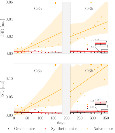
Figure 6: Average (top) and maximum (bottom) JS-divergences over all parameters between Dingo samples and reference samples. Injections use noise PSDs estimated at various times throughout O3 (indicated on horizontal axis). Results are averaged over injections with five random sets of source parameters (fixed for all PSDs). Day 0 marks the beginning of O3a. The gap indicates the period when detectors were offline between O3a and O3b.

Appendix A Additional Results

Figure 6 shows the mean (top) and maximum (bottom) JSDs between various Dingo posteriors and reference samples, across all inferred parameters, for the study on simulated data in Section III.1. We see that the network trained with Synthetic PSDs on average performs similarly to that trained with full PSD information (Oracle), with minor deviations for those parameters that are estimated the worst. The average JSD for the Oracle dataset is $1.6\pm 0.7$ $(\cdot 10^{-3})$ nat, for Synthetic is $2.0\pm 0.9$ $(\cdot 10^{-3})$ nat and for Naive is $19.1\pm 18.8$ $(\cdot 10^{-3})$ nat. In Figure 7, we compare posterior marginal distributions of selected O3 events between the reference posterior and our Dingo models. With the Oracle and Synthetic PSD distributions, we obtain excellent agreement with the reference. Using the Naive noise model, however, can lead to significant deviations.

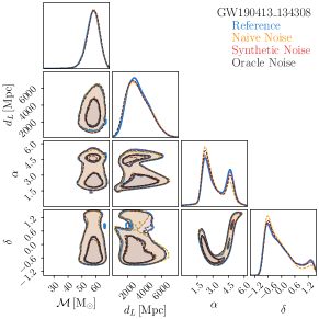
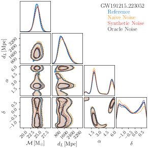
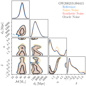
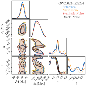
Figure 7: Marginalized one- and two-dimensional posterior distributions for selected O3 events, comparing Dingo models trained with empirically estimated PSDs from the beginning of the observing run (orange), throughout the entire observing run (black) and our proposed synthetic PSD model (red) to the reference posterior (blue, obtained with importance sampling [23]). Contours represent 90% credible regions.

References

- Aasi et al. [2015] J. Aasi et al. (LIGO Scientific), Advanced LIGO, Class. Quant. Grav. 32, 074001 (2015), arXiv:1411.4547 [gr-qc] .
- Acernese et al. [2015] F. Acernese et al. (VIRGO), Advanced Virgo: a second-generation interferometric gravitational wave detector, Class. Quant. Grav. 32, 024001 (2015), arXiv:1408.3978 [gr-qc] .
- Somiya [2012] K. Somiya (KAGRA), Detector configuration of KAGRA: The Japanese cryogenic gravitational-wave detector, Class. Quant. Grav. 29, 124007 (2012), arXiv:1111.7185 [gr-qc] .
- Aso et al. [2013] Y. Aso, Y. Michimura, K. Somiya, M. Ando, O. Miyakawa, T. Sekiguchi, D. Tatsumi, and H. Yamamoto (KAGRA), Interferometer design of the KAGRA gravitational wave detector, Phys. Rev. D 88, 043007 (2013), arXiv:1306.6747 [gr-qc] .
- Akutsu et al. [2021] T. Akutsu et al. (KAGRA), Overview of KAGRA: Detector design and construction history, PTEP 2021, 05A101 (2021), arXiv:2005.05574 [physics.ins-det] .
- Welch [1967] P. Welch, The use of fast fourier transform for the estimation of power spectra: a method based on time averaging over short, modified periodograms, IEEE Transactions on audio and electroacoustics 15, 70 (1967).
- Cornish and Littenberg [2015] N. J. Cornish and T. B. Littenberg, BayesWave: Bayesian Inference for Gravitational Wave Bursts and Instrument Glitches, Class. Quant. Grav. 32, 135012 (2015), arXiv:1410.3835 [gr-qc] .
- Cornish et al. [2021] N. J. Cornish, T. B. Littenberg, B. Bécsy, K. Chatziioannou, J. A. Clark, S. Ghonge, and M. Millhouse, BayesWave analysis pipeline in the era of gravitational wave observations, Phys. Rev. D 103, 044006 (2021), arXiv:2011.09494 [gr-qc] .
- Veitch et al. [2015] J. Veitch et al., Parameter estimation for compact binaries with ground-based gravitational-wave observations using the LALInference software library, Phys. Rev. D91, 042003 (2015), arXiv:1409.7215 [gr-qc] .
- Ashton et al. [2019] G. Ashton et al., BILBY: A user-friendly Bayesian inference library for gravitational-wave astronomy, Astrophys. J. Suppl. 241, 27 (2019), arXiv:1811.02042 [astro-ph.IM] .
- Romero-Shaw et al. [2020] I. M. Romero-Shaw et al., Bayesian inference for compact binary coalescences with bilby: validation and application to the first LIGO–Virgo gravitational-wave transient catalogue, Mon. Not. Roy. Astron. Soc. 499, 3295 (2020), arXiv:2006.00714 [astro-ph.IM] .
- Speagle [2020] J. S. Speagle, dynesty: a dynamic nested sampling package for estimating bayesian posteriors and evidences, Monthly Notices of the Royal Astronomical Society 493, 3132–3158 (2020), arXiv:1904.02180 [astro-ph.IM] .
- Gabbard et al. [2022] H. Gabbard, C. Messenger, I. S. Heng, F. Tonolini, and R. Murray-Smith, Bayesian parameter estimation using conditional variational autoencoders for gravitational-wave astronomy, Nature Phys. 18, 112 (2022), arXiv:1909.06296 [astro-ph.IM] .
- Chua and Vallisneri [2020] A. J. K. Chua and M. Vallisneri, Learning Bayesian posteriors with neural networks for gravitational-wave inference, Phys. Rev. Lett. 124, 041102 (2020), arXiv:1909.05966 [gr-qc] .
- Chatterjee et al. [2019] C. Chatterjee, L. Wen, K. Vinsen, M. Kovalam, and A. Datta, Using Deep Learning to Localize Gravitational Wave Sources, Phys. Rev. D 100, 103025 (2019), arXiv:1909.06367 [astro-ph.IM] .
- Green et al. [2020] S. R. Green, C. Simpson, and J. Gair, Gravitational-wave parameter estimation with autoregressive neural network flows, Phys. Rev. D 102, 104057 (2020), arXiv:2002.07656 [astro-ph.IM] .
- Green and Gair [2021] S. R. Green and J. Gair, Complete parameter inference for GW150914 using deep learning, Mach. Learn. Sci. Tech. 2, 03LT01 (2021), arXiv:2008.03312 [astro-ph.IM] .
- Delaunoy et al. [2020] A. Delaunoy, A. Wehenkel, T. Hinderer, S. Nissanke, C. Weniger, A. R. Williamson, and G. Louppe, Lightning-Fast Gravitational Wave Parameter Inference through Neural Amortization, (2020), arXiv:2010.12931 [astro-ph.IM] .
- Dax et al. [2021] M. Dax, S. R. Green, J. Gair, J. H. Macke, A. Buonanno, and B. Schölkopf, Real-Time Gravitational Wave Science with Neural Posterior Estimation, Phys. Rev. Lett. 127, 241103 (2021), arXiv:2106.12594 [gr-qc] .
- Dax et al. [2022a] M. Dax, S. R. Green, J. Gair, M. Deistler, B. Schölkopf, and J. H. Macke, Group equivariant neural posterior estimation, in International Conference on Learning Representations (ICLR 2022) (2022) arXiv:2111.13139 [cs.LG] .
- Krastev et al. [2021] P. G. Krastev, K. Gill, V. A. Villar, and E. Berger, Detection and Parameter Estimation of Gravitational Waves from Binary Neutron-Star Mergers in Real LIGO Data using Deep Learning, Phys. Lett. B 815, 136161 (2021), arXiv:2012.13101 [astro-ph.IM] .
- Shen et al. [2021] H. Shen, E. A. Huerta, E. O’Shea, P. Kumar, and Z. Zhao, Statistically-informed deep learning for gravitational wave parameter estimation, (2021), arXiv:1903.01998v3 [gr-qc] .
- Dax et al. [2022b] M. Dax, S. R. Green, J. Gair, M. Pürrer, J. Wildberger, J. H. Macke, A. Buonanno, and B. Schölkopf, Neural Importance Sampling for Rapid and Reliable Gravitational-Wave Inference, (2022b), arXiv:2210.05686 [gr-qc] .
- Abbott et al. [2021] R. Abbott et al. (LIGO Scientific, Virgo), Open data from the first and second observing runs of Advanced LIGO and Advanced Virgo, SoftwareX 13, 100658 (2021), arXiv:1912.11716 [gr-qc] .
- Bartholomew et al. [2011] D. J. Bartholomew, M. Knott, and I. Moustaki, Latent variable models and factor analysis: A unified approach (John Wiley & Sons, 2011).
- Kingma and Welling [2014] D. P. Kingma and M. Welling, Auto-Encoding Variational Bayes, in 2nd International Conference on Learning Representations, ICLR 2014, Banff, AB, Canada, April 14-16, 2014, Conference Track Proceedings (2014) http://arxiv.org/abs/1312.6114v10 .
- Rezende et al. [2014] D. J. Rezende, S. Mohamed, and D. Wierstra, Stochastic backpropagation and approximate inference in deep generative models, in International Conference on Machine Learning (2014) pp. 1278–1286, 1401.4082 [stat.ML] .
- Littenberg and Cornish [2014] T. Littenberg and N. Cornish, Bayesline: Bayesian inference for spectral estimation of gravitational wave detector noise, Physical Review D 91 (2014).
- Khan et al. [2016] S. Khan, S. Husa, M. Hannam, F. Ohme, M. Pürrer, X. Jimńez Forteza, and A. Bohé, Frequency-domain gravitational waves from nonprecessing black-hole binaries. II. A phenomenological model for the advanced detector era, Phys. Rev. D93, 044007 (2016), arXiv:1508.07253 [gr-qc] .
- Hannam et al. [2014] M. Hannam, P. Schmidt, A. Bohé, L. Haegel, S. Husa, F. Ohme, G. Pratten, and M. Pürrer, Simple Model of Complete Precessing Black-Hole-Binary Gravitational Waveforms, Phys. Rev. Lett. 113, 151101 (2014), arXiv:1308.3271 [gr-qc] .
- Bohé et al. [2017] A. Bohé et al., Improved effective-one-body model of spinning, nonprecessing binary black holes for the era of gravitational-wave astrophysics with advanced detectors, Phys. Rev. D 95, 044028 (2017), arXiv:1611.03703 [gr-qc] .
- Veitch and Del Pozzo [2013] J. Veitch and W. Del Pozzo, Analytic marginalisation of phase parameter, URL: https://dcc. ligo. org/LIGO-T1300326/public (2013).
- Thrane and Talbot [2019] E. Thrane and C. Talbot, An introduction to Bayesian inference in gravitational-wave astronomy: parameter estimation, model selection, and hierarchical models, Publ. Astron. Soc. Austral. 36, e010 (2019), [Erratum: Publ.Astron.Soc.Austral. 37, e036 (2020)], arXiv:1809.02293 [astro-ph.IM] .
- Lin [1991] J. Lin, Divergence measures based on the Shannon entropy, IEEE Trans. Info. Theor. 37, 145 (1991).
- Romero-Shaw et al. [2020] I. M. Romero-Shaw, C. Talbot, S. Biscoveanu, V. D’Emilio, G. Ashton, C. P. L. Berry, S. Coughlin, S. Galaudage, C. Hoy, M. Hübner, K. S. Phukon, M. Pitkin, M. Rizzo, N. Sarin, R. Smith, S. Stevenson, A. Vajpeyi, M. Arène, K. Athar, S. Banagiri, N. Bose, M. Carney, K. Chatziioannou, J. A. Clark, M. Colleoni, R. Cotesta, B. Edelman, H. Estellés, C. García-Quirós, A. Ghosh, R. Green, C. J. Haster, S. Husa, D. Keitel, A. X. Kim, F. Hernandez-Vivanco, I. Magaña Hernandez, C. Karathanasis, P. D. Lasky, N. De Lillo, M. E. Lower, D. Macleod, M. Mateu-Lucena, A. Miller, M. Millhouse, S. Morisaki, S. H. Oh, S. Ossokine, E. Payne, J. Powell, G. Pratten, M. Pürrer, A. Ramos-Buades, V. Raymond, E. Thrane, J. Veitch, D. Williams, M. J. Williams, and L. Xiao, Bayesian inference for compact binary coalescences with BILBY: validation and application to the first LIGO-Virgo gravitational-wave transient catalogue, MNRAS 499, 3295 (2020), arXiv:2006.00714 [astro-ph.IM] .
- Paszke et al. [2019] A. Paszke, S. Gross, F. Massa, A. Lerer, J. Bradbury, G. Chanan, T. Killeen, Z. Lin, N. Gimelshein, L. Antiga, A. Desmaison, A. Kopf, E. Yang, Z. DeVito, M. Raison, A. Tejani, S. Chilamkurthy, B. Steiner, L. Fang, J. Bai, and S. Chintala, Pytorch: An imperative style, high-performance deep learning library, in Advances in Neural Information Processing Systems 32, edited by H. Wallach, H. Larochelle, A. Beygelzimer, F. d’Alché Buc, E. Fox, and R. Garnett (Curran Associates, Inc., 2019) pp. 8024–8035.
- Durkan et al. [2020] C. Durkan, A. Bekasov, I. Murray, and G. Papamakarios, nflows: normalizing flows in PyTorch (2020).
- LIGO Scientific Collaboration [2018] LIGO Scientific Collaboration, LIGO Algorithm Library - LALSuite, free software (GPL) (2018).
- Kingma and Ba [2014] D. P. Kingma and J. Ba, Adam: A Method for Stochastic Optimization, (2014), arXiv:1412.6980 [cs.LG] .
- Hunter [2007] J. D. Hunter, Matplotlib: A 2d graphics environment, Computing in Science & Engineering 9, 90 (2007).
- Hinton [2016] S. R. Hinton, ChainConsumer, The Journal of Open Source Software 1, 00045 (2016).