Towards Robust Low-Resource Fine-Tuning with
Multi-View Compressed Representations

Abstract

Due to the huge amount of parameters, fine-tuning of pretrained language models (PLMs) is prone to overfitting in the low resource scenarios. In this work, we present a novel method that operates on the hidden representations of a PLM to reduce overfitting. During fine-tuning, our method inserts random autoencoders between the hidden layers of a PLM, which transform activations from the previous layers into multi-view compressed representations before feeding them into the upper layers. The autoencoders are plugged out after fine-tuning, so our method does not add extra parameters or increase computation cost during inference. Our method demonstrates promising performance improvement across a wide range of sequence- and token-level low-resource NLP tasks. Our code is available at https://github.com/DAMO-NLP-SG/MVCR.

1 Introduction

Fine-tuning pretrained language models (PLMs) (Devlin et al., 2019; Conneau and Lample, 2019; Liu et al., 2020) provides an efficient way to transfer knowledge gained from large scale text corpora to downstream NLP tasks, which has achieved state-of-the-art performance on a wide range of tasks (Yang et al., 2019; Yamada et al., 2020; Chi et al., 2021; Sun et al., 2021; Zhang et al., 2021b, a; Chia et al., 2022; Tan et al., 2022; Zhou et al., 2022b). However, most of the PLMs are designed for general purpose representation learning (Liu et al., 2019; Conneau et al., 2020), so the learned representations unavoidably contain abundant features irrelevant to the downstream tasks. Moreover, the PLMs typically possess a huge amount of parameters (often 100+ millions) (Brown et al., 2020; Min et al., 2021), which makes them more expressive compared with simple models, and hence more vulnerable to overfitting noise or irrelevant features during fine-tuning, especially in the low-resource scenarios.

There has been a long line of research on devising methods to prevent large neural models from overfitting. The most common ones can be roughly grouped into three main categories: data augmentation (DeVries and Taylor, 2017; Ding et al., 2020; Liu et al., 2021; Feng et al., 2021; Xu et al., 2023; Zhou et al., 2022c), parameter/activation regularization (Krogh and Hertz, 1991; Srivastava et al., 2014; Lee et al., 2020; Li et al., 2020) and label smoothing (Szegedy et al., 2016; Yuan et al., 2020), which, from bottom to top, operates on data samples, model parameters/activations and data labels, respectively.

Data augmentation methods, such as back-translation (Sennrich et al., 2016) and masked prediction Bari et al. (2021), are usually designed based on our prior knowledge about the data. Though simple, many of them have proved to be quite effective. Activation (hidden representation) regularization methods are typically orthogonal to other methods and can be used together to improve model robustness from different aspects. However, since the neural models are often treated as a black box, the features encoded in hidden layers are often less interpretable. Therefore, it is more challenging to apply similar augmentation techniques to the hidden representations of a neural model.

Prior studies (Yosinski et al., 2015; Allen-Zhu and Li, 2023; Fu et al., 2022) observe that neural models trained with different regularization or initialization can capture different features of the same input for prediction. Inspired by this finding, in this work we propose a novel method for hidden representation augmentation. Specifically, we insert a set of randomly initialized autoencoders (AEs) (Rumelhart et al., 1985; Baldi, 2012) between the layers of a PLM, and use them to capture different features from the original representations, and then transform them into Multi-View Compressed Representations (MVCR) to improve robustness during fine-tuning on target tasks. Given a hidden representation, an AE first encodes it into a compressed representation of smaller dimension $d$, and then decodes it back to the original dimension. The compressed representation can capture the main variance of the data. Therefore, with a set of AEs of varying $d$, if we select a random one to transform the hidden representations in each fine-tuning step, the same or similar input is compressed with varying compression dimensions. And the upper-level PLM layers will be fed with more diverse and compressed representations for learning, which illustrates the “multi-view” concept. We also propose a tailored hierarchical AE to further increase representation diversity. Crucially, after fine-tuning the PLM with the AEs, the AEs can be plugged out, so they do not add any extra parameters or computation during inference.

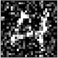
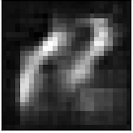
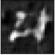
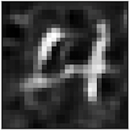
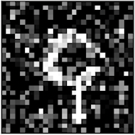
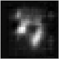
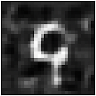
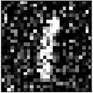
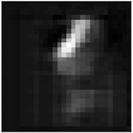
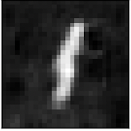
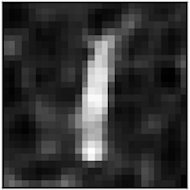
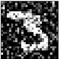
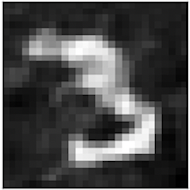
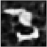
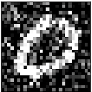
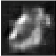
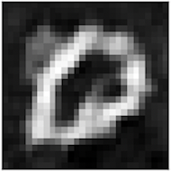
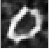
(a) (b) (c) (d)

Figure 1: An illustration of the results reconstructed by autoencoders (AEs) with varying compression ratios: (a) are the inputs (28×28 pixel) to the AEs, and (b) - (d) are the reconstructed images from compressed representations of dimensions 49, 98 and 392, respectively.

We have designed a toy experiment to help illustrate our idea in a more intuitive way. We add uniform random Gaussian noise to the MNIST (LeCun et al., 1998) digits and train autoencoders with different compression ratios to reconstruct the noisy input images. As shown in Fig. 1, the compression dimension $d$ controls the amount of information to be preserved in the latent space. With a small $d$, the AE removes most of the background noise and preserves mostly the crucial shape information about the digits. In Fig. 1b, part of the shape information is also discarded due to high compression ratio. In the extreme case, when $d=1$, the AE would discard almost all of the information from input. Thus, when a small $d$ is used to compress a PLM’s hidden representations during fine-tuning, the reconstructed representations will help: (i) reduce overfitting to noise or task irrelevant features since the high compression ratio can help remove noise; (ii) force the PLM to utilize different relevant features to prevent it from becoming overconfident about a certain subset of them. Since the AE-reconstructed representation may preserve little information when $d$ is small (Fig. 1b), the upper layers are forced to extract only relevant features from the limited information. Besides, the shortcut learning problem (Geirhos et al., 2020) is often caused by learning features that fail to generalize, for example relying on the grasses in background to predict sheep. Our method may force the model to use the compressed representation without grass features. Therefore, it is potentially helpful to mitigate shortcut learning. As shown in Fig. 1(d), with a larger $d$, most information about the digits can be reconstructed, and noises also start to appear in the background. Hence, AEs with varying $d$ can transform a PLM’s hidden representations into different views to increase diversity.

We conduct extensive experiments to verify the effectiveness of MVCR. Compared to many strong baseline methods, MVCR demonstrates consistent performance improvement across a wide range of sequence- and token-level tasks in low-resource adaptation scenarios. We also present abundant ablation studies to justify the design. In summary, our main contributions are:

• Propose a novel method to improve low-resource fine-tuning, which leverages AEs to transform representations of a PLM into multi-view compressed representations to reduce overfitting.

• Design an effective hierarchical variant of the AE to introduce more diversity in fine-tuning.

• Present a plug-in and plug-out fine-tuning approach tailored for our method, which does not add extra parameter or computation during inference.

• Conduct extensive experiments to verify the effectiveness of our method, and run ablation studies to justify our design.

2 Related Work

Overfitting is a long-standing problem in large neural model training, which has attracted broad interest from the research communities (Sarle et al., 1996; Hawkins, 2004; Salman and Liu, 2019; Santos and Papa, 2022; Hu et al., 2023; He et al., 2021b). To better capture the massive information from large-scale text corpora during pretraining, the PLMs are often over-parameterized, which makes them prone to overfitting. The commonly used methods to reduce overfitting can be grouped into three main categories: data augmentation, parameter regularization, and label smoothing.

Data augmentation methods (DeVries and Taylor, 2017; Liu et al., 2021; Feng et al., 2021) are usually applied to increase training sample diversity. Most of the widely used methods, such as synonym replacement (Karimi et al., 2021), masked prediction Bari et al. (2021) and back-translation (Sennrich et al., 2016), fall into this category. Label smoothing methods (Szegedy et al., 2016; Yuan et al., 2020) are applied to the data labels to prevent overconfidence and to encourage smoother decision boundaries. Some hybrid methods, like MixUp (Zhang et al., 2018; Verma et al., 2019), are proposed to manipulate both data sample and label, or hidden representation and label. Most parameter/hidden representation regularization methods are orthogonal to the methods discussed above, so they can be used as effective complements.

Neural models are often treated as a black box, so it is more challenging to design efficient parameter or hidden representation regularization methods. Existing methods mainly focus on reducing model expressiveness or adding noise to hidden representations. Weight decay (Krogh and Hertz, 1991) enforces $L_{2}$ norm of the parameters to reduce model expressiveness. Dropout Srivastava et al. (2014) randomly replaces elements in hidden representations with $0$, which is believed to add more diversity and prevent overconfidence on certain features. Inspired by dropout, Mixout (Lee et al., 2020) stochastically mixes the current and initial model parameters during training. Mahabadi et al. (2021) leverage variational information bottleneck (VIB) (Alemi et al., 2017) to help models to learn more concise and task relevant features. However, VIB is limited to regularize last layer sequence-level representations only, while our method can be applied to any layer, and also supports token-level tasks like NER and POS tagging.

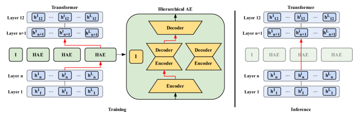
Figure 2: Illustration of token-level Multi-View Compressed Representations (MVCR) with three stochastic hierarchical autoencoders (HAEs) inserted between the transformer layers. During training, the output of layer $n$ is either passed through a randomly selected HAE or directly passed to layer $n+1$ (denoted as “I” in the figure). If an HAE is picked, the output of the outer encoder is either passed through a randomly selected sub-AE or directly passed to the outer decoder (via “I”). In inference, we drop MVCR without adding parameters to the original PLM.

3 Methodology

We first formulate using neural networks over the hidden representation of different layers of deep learning architectures as effective augmentation modules (section 3.1) and then devise a novel hierarchical autodencoder (HAE) to increase stochasticity and diversity (section 3.2). We utilise our novel HAE as a compression module for hidden representations within PLMs, and introduce our method Multi-View Compressed Representation (MVCR) (section 3.3). We finally discuss the training, inference, and optimization of MVCR. An overview of MVCR is presented in Fig. 2.

3.1 Generalizing Neural Networks as Effective Augmentation Modules

Data augmentation Simard et al. (1998) aims at increasing the diversity of training data while preserving quality for more generalized training Shorten and Khoshgoftaar (2019). It can be formalized by the Vicinal Risk Minimization principle Chapelle et al. (2001), which aims to enlarge the support of the training distribution by generating new data points from a vicinity distribution around each training example Zhang et al. (2018). We conjecture that shallow neural networks can be used between the layers of large-scale PLMs to construct such vicinity distribution in the latent space to facilitate diversity and generalizability.

We consider a neural network $g(\cdot)$, and denote its forward pass $F(\cdot)$ for an input ${\bm{x}}$ with $F({\bm{x}})=g({\bm{x}})$. We denote a set of $M$ such networks with $\mathcal{G}=\{g_{1}(\cdot),\dots,g_{M}(\cdot)\}$, where each candidate network $g_{i}(\cdot)$ outputs a different "view" of a given input. We treat ${\mathcal{G}}$ as a stochastic network and define a stochastic forward pass $F^{S}(\cdot,\mathcal{G})$, where a candidate network $g_{i}(\cdot)$ is randomly chosen from the pool $\mathcal{G}$ in each step, enabling diversity due to different non-linear transformations. Formally, for an input ${\bm{x}}$, we obtain the output ${\bm{o}}$ of network $g_{i}(\cdot)$ using $F^{S}$ as,

$${\bm{o}}=F^{S}({\bm{x}},\mathcal{G})=g_{i}({\bm{x}}),\quad i\in\{1,\dots,M\}$$ (1)

For a chosen candidate network $g_{i}$, the output ${\bm{o}}$ represents a network dependent “view” of input ${\bm{x}}$.

We now formalize using $g(\cdot)$ over the hidden representation of large-scale PLMs for effective generalization. Let $f(\cdot)$ denote any general transformer-based PLM containing $N$ hidden layers with $f_{n}(\cdot)$ being the $n$-th layer and ${\bm{h}}_{n}$ being the activations at that layer for $n\in\{1,\dots,N\}$, and let ${\bm{h}}_{0}$ denote the input embeddings. We consider a set of layers ${\mathcal{L}}\subset\{1,\dots,N\}$ where we insert our stochastic network $\mathcal{G}$ for augmenting the hidden representations during the forward pass. To this end, we substitute the standard forward pass of the PLM $f(\cdot)$ during the training phase with the stochastic forward pass $F^{S}(\cdot,\mathcal{G})$. Formally,

$${\bm{h}}_{n}=\begin{cases}F^{S}(f_{n}({\bm{h}}_{n-1}),\mathcal{G}_{n}),&n\in\mathcal{L}\\ f_{n}({\bm{h}}_{n-1}),&n\notin\mathcal{L}\end{cases}$$ (2)

We now devise a novel hierarchical autoencoder network which can be effectively used for augmenting hidden representations of large-scale PLMs.

3.2 Stochastic Hierarchical Autoencoder

Autoencoders (AEs) are a special kind of neural networks where the input dimension is the same as the output dimension Rumelhart et al. (1985). For an input ${\bm{x}}\in\mathbb{R}^{d}$, we define a simple autoencoder $\mathrm{AE}_{d,\hat{d}}(\cdot)$ with compression dimension $\hat{d}$ as a sequential combination of a feed-forward down-projection layer $D_{d,\hat{d}}(\cdot)$ and an up-projection layer $U_{\hat{d},d}(\cdot)$. Given input ${\bm{x}}$, the output ${\bm{o}}\in\mathbb{R}^{d}$ of the autoencoder can be represented as:

$${\bm{o}}=\mathrm{AE}_{d,\hat{d}}({\bm{x}})=U(D({\bm{x}}))$$ (3)

Hierarchical Autoencoder (HAE)

We extend a standard autoencoder to a hierarchical autoencoder and present its overview in Fig. 2 (Hierarchical AE). We do this by inserting a sub-autoencoder $\mathrm{AE}_{\hat{d},d^{\prime}}(\cdot)$ with compression dimension $d^{\prime}$ within an autoencoder $\mathrm{AE}_{d,\hat{d}}(\cdot)$, where $d^{\prime}<\hat{d}$. For $\mathrm{AE}_{\hat{d},d^{\prime}}(\cdot)$, the down- and up-projection layers are denoted with $D^{\prime}_{\hat{d},d^{\prime}}(\cdot)$ and $U^{\prime}_{d^{\prime},\hat{d}}(\cdot)$, respectively. We obtain output ${\bm{o}}\in\mathbb{R}^{d}$ for hierarchical autodencoder $\mathrm{HAE}_{d,\hat{d},d^{\prime}}(\cdot)$ as,

$$\begin{split}{\bm{o}}\!=\!\mathrm{HAE}_{d,\hat{d},d^{\prime}}({\bm{x}})\!&=\!U(\mathrm{AE}_{\hat{d},d^{\prime}}(D({\bm{x}})))\\ \!&=\!U(U^{\prime}(D^{\prime}(D({\bm{x}}))))\\ \end{split}$$ (4)

Note that, HAEs are different from the AEs having multiple encoder and decoder layers, since it also enforces reconstruction loss on the outputs of $D({\bm{x}})$ and $U^{\prime}(D^{\prime}(D({\bm{x}})))$ as expressed in Eq. 4. Thus HAEs can compress representations step by step, and provides flexibility to reconstruct the inputs with or without the sub-autoencoders. By sharing the outer layer parameters of a series of inner AEs, HAE can introduce more diversity without adding significant parameters and training overhead.

Stochastic Hierarchical Autoencoder

We use a stochastic set of sub-autoencoders $\mathcal{E}_{\hat{d}}$ within an HAE to formulate a stochastic hierarchical autoencoder, where $\hat{d}$ is the input dimension of the sub-autoencoders. While performing the forward pass of the stochastic hierarchical autoencoder, we randomly choose one sub-autoencoder $\mathrm{AE}_{\hat{d},d_{i}}\in\mathcal{E}_{\hat{d}}$ within the autoencoder $\mathrm{AE}_{d,\hat{d}}$. We set the compression dimension $d_{i}=\hat{d}/2$. Hence, for an input ${\bm{x}}\in\mathbb{R}^{d}$, the output ${\bm{o}}\in\mathbb{R}^{d}$ of a stochastic hierarchical autoencoder $\mathrm{HAE}^{S}_{d,\hat{d}}$ is given by

$$\begin{split}{\bm{o}}&=\mathrm{HAE}^{S}_{d,\hat{d}}({\bm{x}})\\ &=\begin{cases}U(\mathrm{AE}_{\hat{d},d_{i}}(D({\bm{x}}))),&z>0.3\\ U(D({\bm{x}})),&z\leq 0.3\end{cases}\end{split}$$ (5)

where $z$ is uniformly sampled from the range $[0,1]$, and $\mathrm{AE}_{\hat{d},d_{i}}\in\mathcal{E}_{\hat{d}}$ is randomly selected in each step. So for 30% of the time, we do not use the sub-autoencoders. These randomness introduces more diversity to the generated views to reduce overfitting. For the stochastic HAE, we only compute the reconstruction loss between ${\bm{x}}$ and ${\bm{o}}$, since this also implicitly minimizes the distance between $\mathrm{AE}_{\hat{d},d_{i}}(D({\bm{x}}))$ and $D({\bm{x}})$ in Eq. 5. See §A.2 for detailed explanation. In the following sections, we use HAE to denote stochastic hierarchical autoencoder. We also name the hyper-parameter $\hat{d}$ as HAE compression dimension.

3.3 Multi-View Compressed Representation

Autoencoders can represent data effectively as compressed vectors that capture the main variability in the data distribution Rumelhart et al. (1985). We leverage this capability of autoencoders within our proposed stochastic networks to formulate Multi-View Compressed Representation (MVCR).

We give an illustration of MVCR in Fig. 2. We insert multiple stochastic HAEs (section 3.2) between multiple layers of a PLM (shown for one layer in the figure). Following section 3.1, we consider the Transformer-based PLM $f(\cdot)$ with hidden dimension $d$ and $N$ layers. At layer $n$, we denote the set of stochastic HAEs with $\mathrm{HAE}^{S,n}=\{\mathrm{HAE}^{S,n}_{d,\hat{d}_{1}},\mathrm{HAE}^{S,n}_{d,\hat{d}_{2}},\dots,\mathrm{HAE}^{S,n}_{d,\hat{d}_{M}}\}$, where $M$ is total the number of HAEs. To prevent discarding useful information in the compression process and for more stable training, we only use them for 50% of the times. We modify the forward pass of $f(\cdot)$ with MVCR, denoted by $F^{\mathrm{MVCR}}(\cdot,\mathrm{HAE}^{S,n})$ to obtain the output ${\bm{h}}_{n}$ for an input ${\bm{h}}_{n-1}$ as

$$\begin{split}{\bm{h}}_{n}&=F^{\mathrm{MVCR}}({\bm{h}}_{n-1},\mathrm{HAE}^{S,n})\\ &=\begin{cases}F^{S}(f_{n}({\bm{h}}_{n-1}),\mathrm{HAE}^{S,n}),&z\leq 0.5\\ f_{n}({\bm{h}}_{n-1}),&z>0.5\end{cases}\end{split}$$ (6)

where $z$ is uniformly sampled from the range $[0,1]$. Following Eq. 2, we finally define $\mathrm{MVCR}(\cdot,\mathrm{HAE}^{S})$ for a layer set $\mathcal{L}$ of a PLM to compute the output ${\bm{h}}_{n}$ using stochastic HAEs as

$$\begin{split}{\bm{h}}_{n}&=\mathrm{MVCR}({\bm{h}}_{n-1},\mathrm{HAE}^{S})\\ &=\begin{cases}F^{\mathrm{MVCR}}(f_{n}({\bm{h}}_{n-1}),\mathrm{H}^{S,n}),&n\in\mathcal{L}\\ f_{n}({\bm{h}}_{n-1}),&n\notin\mathcal{L}\end{cases}\end{split}$$ (7)

Note that MVCR can be used either at layer-level or token-level. At layer-level, all of the hidden (token) representations in the same layer are augmented with the same randomly selected HAE in each training step. At token-level, each token representation can select a random HAE to use. We show that token-level MVCR performs better than layer-level on account of more diversity and stochasticity (section 5) and choose this as the default setup.

Network Optimization

We use two losses for optimizing MVCR. Firstly, our method do not make change to the task layer, so the original task-specific loss $\mathcal{L}_{\text{task}}$ is used to update the PLM, task layer, and HAE parameters. We use a small learning rate $\alpha_{\text{task}}$ to minimize $\mathcal{L}_{\text{task}}$. Secondly, to increase training stability, we also apply reconstruction loss $\mathcal{L}_{\mathrm{MSE}}$ to the output of HAEs to ensure the augmented representations are projected to the space not too far from the original one. At layer $n$, we have

$$\mathcal{L}_{\mathrm{MSE}}=\frac{1}{M\times L}\sum_{m=1}^{M}\sum_{i=1}^{L}({\bm{h}}_{n}^{i}-\mathrm{HAE}_{m}({\bm{h}}_{n}^{i}))^{2}$$ (8)

where $M$ is the number of HAEs on each layer, and $L$ is the PLM input sequence length (in tokens). We use a larger learning rate $\alpha_{\mathrm{MSE}}$ to optimize $\mathcal{L}_{\mathrm{MSE}}$ since the HAEs are randomly initialized. This reconstruction loss not only increases training stability, but also allows us to plug-out the HAEs during inference, since it ensures that the generated views are close to the original hidden representation.

4 Experiments

In this section, we present the experiments designed to evaluate our method. We first describe the baselines and training details, followed by the evaluation on both the sequence- and token-level tasks across six (6) different datasets.

Baselines

We compare our method with several widely used parameter and hidden representation regularization methods, including Dropout (Srivastava et al., 2014), Weight Decay (WD) (Krogh and Hertz, 1991) and Gaussian Noise (GN) (Kingma and Welling, 2013). Some more recent methods are also included for more comprehensive comparison, such as Adapter (Houlsby et al., 2019), Mixout (Lee et al., 2020), as well as the variational information bottleneck (VIB) based method proposed by Mahabadi et al. (2021). More information about these baselines can be found in §A.3. In this paper, we focus on regularization methods for hidden representation. Thus, we do not compare with data augmentation methods which improve model performance from a different aspect.

Method	full	100	200	500	1000	$\text{avg}_{low}$
SNLI
BERT	90.28 (0.1)	48.93 (1.9)	58.46 (0.9)	66.46 (1.2)	72.57 (0.5)	61.61
Dropout	90.20 (0.4)	48.16 (3.4)	59.47 (1.3)	67.10 (1.8)	73.10 (0.3)	61.96
WD	90.44 (0.3)	47.37 (4.6)	59.10 (0.3)	66.59 (1.3)	73.41 (0.7)	61.62
GN	90.23 (0.0)	49.01 (5.6)	58.86 (0.6)	66.46 (1.9)	73.02 (0.3)	61.84
Adapter	90.11 (0.0)	48.88 (1.0)	58.99 (0.6)	65.80 (0.8)	73.67 (0.5)	61.84
Mixout	89.97 (0.4)	49.57 (1.4)	57.31 (3.0)	63.46 (1.7)	71.09 (0.9)	60.36
VIB	90.11 (0.1)	49.46 (1.9)	59.14 (1.7)	66.21 (0.6)	73.87 (1.0)	62.17
MVCR1	90.64 (0.2)	51.73 (0.3)	61.50 (0.1)	67.26 (0.1)	74.41 (0.1)	63.73
MVCR12	90.57 (0.2)	49.99 (1.0)	59.45 (0.1)	67.93 (0.4)	73.85 (1.0)	62.81
MNLI
BERT	83.91 (0.5)	37.27 (4.6)	45.60 (1.3)	53.22 (2.3)	58.58 (1.5)	48.67
Dropout	83.94 (0.5)	37.97 (1.8)	43.31 (0.5)	52.57 (1.6)	59.25 (2.5)	48.28
WD	84.27 (0.2)	38.05 (5.5)	45.57 (1.3)	52.83 (1.8)	58.61 (1.1)	48.76
GN	84.00 (0.1)	38.05 (5.3)	45.60 (1.4)	53.20 (1.4)	58.93 (0.5)	48.95
Adapter	83.35 (0.0)	36.61 (4.5)	45.28 (2.9)	55.27 (0.3)	59.30 (1.9)	49.12
Mixout	83.80 (0.2)	36.61 (4.2)	44.92 (1.6)	52.89 (0.9)	54.88 (1.5)	47.33
VIB	84.32 (0.1)	39.34 (1.8)	45.05 (0.9)	52.23 (0.2)	52.40 (0.3)	47.26
MVCR1	84.47 (0.1)	40.19 (1.1)	46.84 (0.9)	56.43 (1.3)	59.71 (1.7)	50.79
MVCR12	84.42 (0.2)	39.61 (2.0)	45.94 (1.0)	57.02 (1.6)	60.35 (0.9)	50.73
MNLI-mm
BERT	84.32 (0.6)	38.69 (3.0)	46.20 (1.7)	53.44 (2.3)	59.88 (1.8)	49.55
Dropout	84.44 (0.4)	38.84 (3.0)	44.14 (1.0)	53.60 (2.8)	60.31 (1.8)	49.22
WD	84.57 (0.3)	39.52 (1.8)	46.22 (1.8)	53.40 (2.0)	60.26 (1.6)	49.85
GN	84.33 (0.2)	40.21 (2.5)	47.00 (0.9)	53.51 (0.3)	60.22 (0.9)	50.23
Adapter	84.01 (0.1)	39.57 (0.8)	46.64 (1.7)	54.87 (0.9)	59.84 (3.2)	50.23
Mixout	84.10 (0.2)	39.88 (1.1)	46.22 (1.2)	53.48 (0.5)	56.09 (0.5)	48.92
VIB	84.65 (0.2)	40.49 (2.2)	45.76 (0.2)	54.62 (1.7)	54.45 (0.7)	48.83
MVCR1	84.72 (0.1)	41.75 (0.6)	48.33 (0.9)	56.45 (1.2)	61.09 (0.5)	51.90
MVCR12	84.68 (0.2)	41.82 (0.4)	48.32 (1.3)	57.87 (1.5)	60.91 (1.3)	52.23

Table 1: Experimental results (Acc.) on the natural language inference (NLI) tasks. $\text{avg}_{low}$ is the average result of low-resource scenarios.

Method	full	100	200	500	1000	$\text{avg}_{low}$
IMDb
BERT	88.47 (0.6)	72.04 (4.8)	79.01 (4.3)	81.16 (0.8)	84.24 (0.5)	79.11
Dropout	88.93 (0.1)	75.89 (2.7)	79.76 (2.0)	82.19 (0.2)	83.85 (0.6)	80.42
WD	88.73 (0.6)	73.74 (4.2)	79.61 (3.2)	81.90 (0.7)	84.00 (0.4)	79.81
GN	88.85 (0.1)	74.17 (2.1)	79.49 (2.8)	82.10 (0.6)	84.04 (0.2)	79.95
Adapter	88.39 (0.0)	73.28 (3.1)	80.18 (0.4)	81.54 (0.6)	83.19 (0.3)	79.55
Mixout	88.46 (0.2)	66.04 (3.0)	78.84 (3.8)	81.33 (0.8)	83.64 (0.3)	77.46
VIB	88.73 (0.1)	73.67 (2.2)	79.63 (2.8)	82.53 (0.1)	83.78 (0.8)	79.90
MVCR1	89.01 (0.1)	76.30 (2.1)	81.76 (0.1)	83.22 (0.4)	84.38 (0.2)	81.41
MVCR12	88.73 (0.1)	77.23 (1.8)	80.64 (1.3)	83.15 (0.3)	84.19 (0.4)	81.30
Yelp
BERT	62.01 (0.4)	40.79 (0.2)	42.43 (2.7)	46.93 (2.3)	51.17 (1.9)	45.33
Dropout	62.05 (0.4)	40.55 (1.3)	40.05 (0.4)	48.26 (1.8)	51.94 (1.3)	45.20
WD	61.62 (0.2)	40.86 (0.2)	41.46 (3.5)	47.04 (3.1)	50.74 (0.8)	45.02
GN	62.12 (0.0)	40.46 (0.8)	41.36 (0.5)	46.07 (2.5)	51.90 (0.9)	44.95
Adapter	61.67 (0.3)	39.58 (0.8)	41.05 (0.8)	47.49 (1.8)	50.26 (0.9)	44.60
Mixout	61.50 (0.6)	40.75 (0.3)	40.68 (2.9)	45.41 (1.8)	49.33 (1.8)	44.04
VIB	60.65 (0.4)	40.84 (0.8)	41.21 (0.9)	45.59 (2.7)	50.22 (3.0)	44.46
MVCR1	62.26 (0.3)	42.75 (0.2)	43.74 (0.2)	48.50 (0.8)	52.68 (0.6)	46.92
MVCR12	62.42 (0.1)	41.83 (1.0)	43.10 (0.7)	48.02 (1.0)	52.81 (0.4)	46.44

Table 2: Experimental results (Acc.) on the IMDb and Yelp text classification tasks. $\text{avg}_{low}$ is the average result of low-resource scenarios.

Training Details

Same as Mahabadi et al. (2021), we fine-tune $\text{BERT}_{\textrm{base}}$ (Devlin et al., 2019) for the sequence-level tasks. The token-level tasks are multilingual, so we tune $\text{XLM-R}_{\textrm{base}}$ (Conneau et al., 2020) on them. We use $\text{MVCR}_{l}$ to denote our methods, where $l$ is the PLM layer that we insert HAEs. For example in $\text{MVCR}_{1}$, the HAEs are inserted after the 1st transformer layer. On each layer, we insert three HAEs with compressed representation dimensions 128, 256 and 512, respectively. All HAEs are discarded during inference. For each experiment, we report the average result of 3 runs.

For each dataset, we randomly sample 100, 200, 500 and 1000 instances from the training set to simulate the low-resource scenarios. The same amount of instances are also sampled from the dev sets for model selection. The full test set is used for evaluation. More details can be found in §A.5.

4.1 Results of Sequence-Level Tasks

For the sequence-level tasks, we experiment with two natural language inference (NLI) benchmarks, namely SNLI (Bowman et al., 2015) and MNLI (Williams et al., 2018), and two text classification tasks, namely IMDb (Maas et al., 2011) and Yelp (Zhang et al., 2015). Since MNLI has matched and mismatched versions, we report the results on each of them separately.

We present the experimental results for the NLI tasks in Table 1, and text classification tasks in Table 2. $\text{MVCR}_{1}$ and $\text{MVCR}_{12}$ are our methods that insert HAEs after the 1st and 12th transformer layer, respectively. We have the following observations: (a) $\text{MVCR}_{1}$ and $\text{MVCR}_{12}$ consistently outperform all the baselines in the low-resource settings, demonstrating the effectiveness of our method. (b) In very low-resource settings such as with 100 and 200 training samples, $\text{MVCR}_{1}$ often performs better than $\text{MVCR}_{12}$. This indicates that bottom-layer hidden representation augmentation is more efficient than top-layer regularization on extreme low-resource data. We attribute this to the fact that the bottom-layer augmentation impacts more parameters on the top layers. (c) We observe that MVCR outperforms strong baselines, such as VIB. We believe this is due to the fact that MVCR acts as the best-of-both-worlds. Specifically, it acts as a data augmentation module promoting diversity while also acts as a lossy compression module that randomly discards features to prevent overfitting.

4.2 Results of Token-Level Tasks

For token-level tasks, we evaluate our methods on WikiAnn (Pan et al., 2017) for NER and Universal Dependencies v2.5 (Nivre et al., 2020) for POS tagging. Both datasets are multilingual, so we conduct experiments in the zero-shot cross-lingual setting, where all models are fine-tuned on English first and then evaluated on the other languages directly.

As shown in Table 3, our methods are also proven to be useful on the token-level tasks. $\text{MVCR}_{2,12}$ is our method that inserts HAEs after both the 2nd and 12th transformer layers. Comparing the results of $\text{MVCR}_{2}$ and $\text{MVCR}_{2,12}$, we can see adding one more layer of HAEs indeed leads to consistent performance improvement on WikiAnn. However, $\text{MVCR}_{2}$ performs better on the POS tagging task. We also observe that Mixout generally does not perform well when the number of training samples is very small. Detailed analysis about HAE insertion layers is presented in §5.

Method	full	100	200	500	1000	$\text{avg}_{low}$
WikiAnn
XLM-R	59.67 (0.5)	46.90 (1.0)	50.77 (0.4)	52.69 (0.3)	55.45 (0.4)	51.45
Dropout	59.98 (0.4)	47.30 (0.9)	50.09 (0.8)	53.20 (0.2)	55.10 (0.3)	51.42
WD	58.86 (0.6)	46.86 (1.2)	50.46 (0.8)	53.28 (1.3)	55.29 (0.6)	51.47
GN	59.40 (0.6)	47.82 (0.9)	50.94 (0.7)	52.89 (0.4)	54.29 (0.5)	51.48
Adapter	59.31 (0.3)	45.65 (0.6)	48.17 (0.6)	51.26 (0.3)	54.06 (0.5)	49.79
Mixout	59.32 (0.5)	43.14 (0.7)	43.92 (0.9)	50.67 (0.5)	50.89 (0.3)	47.15
MVCR2	60.33 (0.3)	47.35 (0.7)	51.43 (0.5)	53.93 (0.3)	55.72 (0.6)	52.11
MVCR2,12	60.65 (0.4)	48.16 (0.7)	51.26 (0.7)	54.43 (0.4)	56.10 (0.5)	52.49
POS
XLM-R	72.76 (0.2)	70.52 (0.5)	70.87 (0.3)	72.23 (0.3)	72.37 (0.4)	71.50
Dropout	73.03 (0.1)	70.25 (0.7)	71.22 (0.3)	72.02 (0.2)	72.67 (0.2)	71.54
WD	72.76 (0.4)	70.44 (0.5)	71.21 (0.5)	72.14 (0.6)	72.58 (0.4)	71.59
GN	72.96 (0.2)	70.47 (0.6)	71.47 (0.2)	72.48 (0.4)	72.43 (0.1)	71.70
Adapter	72.70 (0.3)	70.65 (0.4)	71.07 (0.3)	72.08 (0.6)	71.75 (0.3)	71.39
Mixout	72.84 (0.1)	68.38 (0.8)	69.20 (0.4)	70.73 (0.2)	71.23 (0.6)	69.89
MVCR2	73.05 (0.1)	71.12 (0.5)	71.33 (0.4)	72.78 (0.3)	73.13 (0.3)	72.09
MVCR2,12	72.78 (0.2)	70.93 (0.4)	71.25 (0.3)	72.49 (0.5)	72.56 (0.2)	71.81

Table 3: Zero-shot cross-lingual NER and POS tagging results (F1-score). $\text{avg}_{low}$ is the average result of low-resource scenarios.

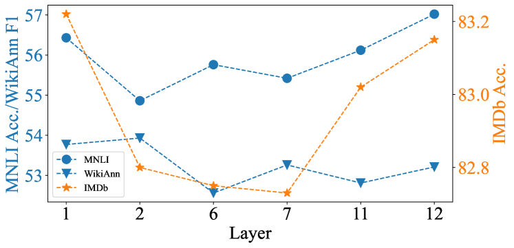
Figure 3: Results on adding the one-layer MVCR after different transformer layers, where bottom and top layers show better results for both sequence- and token-level tasks.

5 Analysis and Ablation Studies

To better understand the improvements obtained by MVCR, we conduct in-depth analysis and ablation studies. We experiment with both sequence- and token-level tasks by sampling 500 instances from 3 datasets, namely MNLI, IMDb and WikiAnn.

$\bullet$ Insertion Layer(s) of MVCR

Based on (Clark et al., 2019), each layer in BERT captures different type of information, such as surface, syntactic or semantic information. Same as above, we fix the dimensions of the three HAEs on each layer to 128, 256 and 512. To comprehensively analyse the impact of adding MVCR after different layers, we select two layers for bottom, middle and top layers. More specifically, {1, 2} for bottom, {6, 7} for middle and {11, 12} for top layers.

As shown in Fig. 3, adding MVCR after layer 1 or 12 achieves the best performance than the other layers. This result can be explained in the way of different augmentation methods (Feng et al., 2021). By adding MVCR after layer 1, the module acts as a data generator which creates multi-view representation inputs to all the upper layers. While adding MVCR after layer 12, which is more relevant to the downstream tasks, the module focuses on preventing the task layer from overfitting (Zhou et al., 2022a). Apart from one layer, we also experiment with adding MVCR to a combination of two layers (Table 4 and Table 5). For token-level task, adding MVCR to both layer 2 and 12 performs even better than one layer. However, it does not help improve the performance on sequence-level tasks. Similar to the $\beta$ parameter in VIB (Mahabadi et al., 2021) which controls the amount of random noise added to the representation, the number of layers in MVCR controls the trade-off between adding more variety to the hidden representation and keeping more information from the original representation. And the optimal trade-off point can be different for sequence- and token-level tasks.

Layer	1	2	6	7	11	12
MNLI	56.43	54.86	55.76	55.42	56.12	57.02
IMDb	83.22	82.80	82.75	82.73	83.02	83.15
Layer	1,2	1,3	1,6	1,7	1,11	1,12
MNLI	49.94	48.63	50.38	50.73	50.52	51.10
IMDb	82.59	82.73	82.57	82.64	82.50	82.36

Table 4: HAE insertion layers for sequence-level tasks.

Layer	1	2	6	7	11	12
WikiAnn	53.77	53.93	52.56	53.26	52.81	53.21
Layer	2,1	2,3	2,6	2,7	2,11	2,12
WikiAnn	53.57	53.76	53.15	54.29	53.87	54.43

Table 5: HAE insertion layers for token-level task.

$\bullet$ Number of HAEs in MVCR

We analyse the impact of the number of HAEs in MVCR on the diversity of augmenting hidden representations. We fix the compression dimension of HAE’s outer encoder to 256, and only insert HAEs to the bottom layers, layer 1 for MNLI and IMDb, and layer 2 for WikiAnn. As shown in Fig. 4, the performance improves with an increasing number of HAEs, which indicates that adding more HAEs leads to more diversity and better generalization. However, the additional performance gain is marginal after three HAEs. This is probably because without various compressed dimensions, the variety only comes from different initialization of HAEs which can only improve the performance to a limited extent. Hence, we fix the number of HAEs to three for other experiments, including the main experiments.

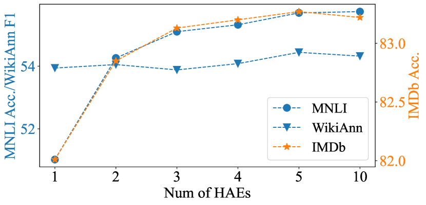
Figure 4: Impact of the number of HAEs in MVCR.

$\bullet$ Diversity of HAE Dimensions

The compression dimensions of HAEs control the amount of information to be passed to upper PLM layers, so using HAEs of varying dimensions may help generate more diverse views during training. To analyse the impact of the compression dimension diversity, we run experiments of three types of combinations: “aaa”, “aab” and “abc”, which contains one, two and three unique dimensions respectively. We compute the average performance of the HAEs with dimensions {32,32,32} to {512,512,512} for “aaa”. We sample the dimensions for “aab” and “abc” since there are too many possible combinations. As we can see from Fig. 5, “abc” consistently outperforms “aab”, while “aab” consistently outperforms “aaa”, which indicates increasing compression dimension diversity can help further improve model generalization.

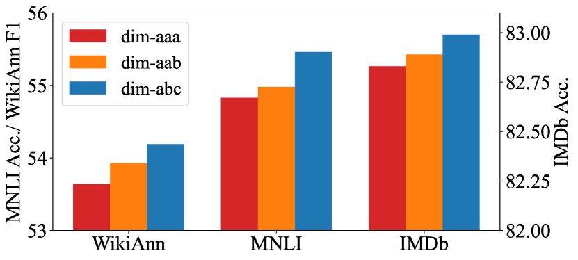
Figure 5: Results on three types of HAE compression dimension combinations: “aaa”, “aab” and “abc”.

$\bullet$ HAE vs. AE vs. VAE

HAEs in MVCR serve as a bottleneck to generate diverse compressed views of the original hidden representations. There are many other possible alternatives for HAE, so we replace HAE with the vanilla AE and variational autoencoder (VAE) (Kingma and Welling, 2014) for comparison. The results in Fig. 6 show that HAE consistently outperforms AE and VAE.

(a) MNLI

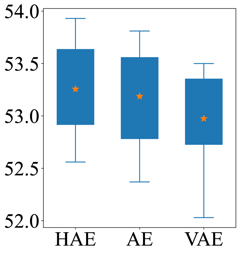
(b) WikiAnn

Figure 6: Results on different types of autoencoders in MVCR. IMDb results can be found in §A.7.

$\bullet$ Token-Level vs. Layer-Level MVCR

In our method, the selection of random HAE can be on token-level or layer-level. For token-level MVCR, each token in the layer randomly selects an HAE from the pool, with the parameters shared within the same layer. Compared with layer-level MVCR, token-level MVCR adds more variety to the model, leading to better results as observed in Fig. 7.

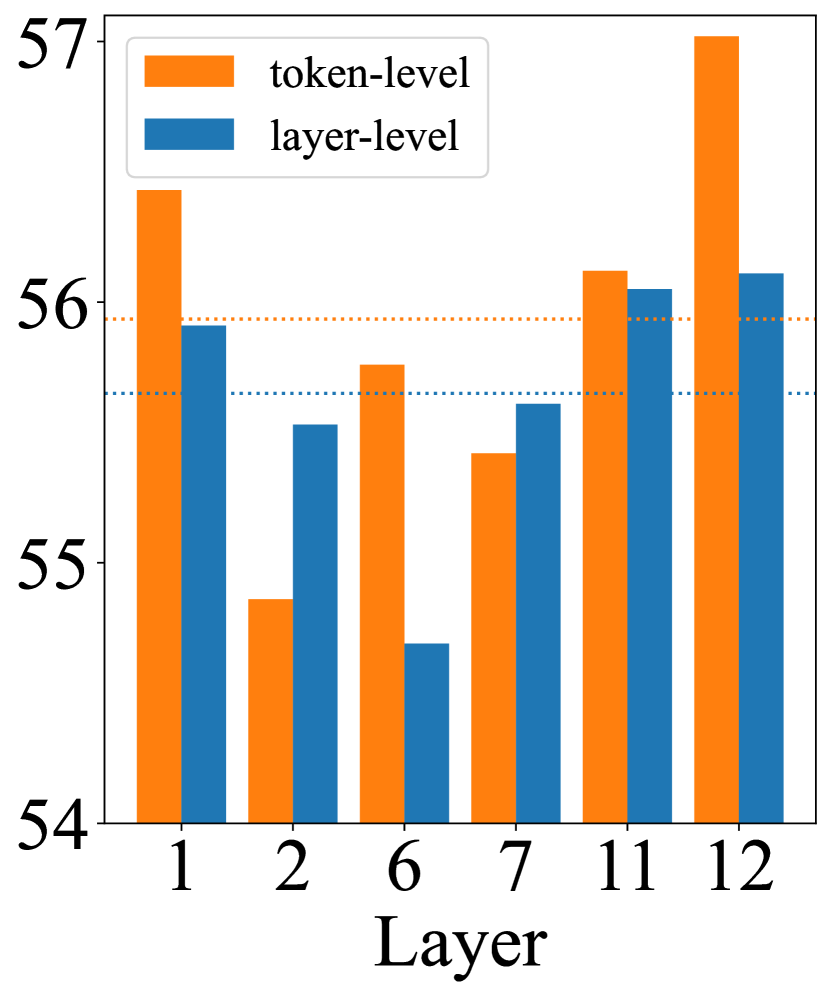
(a) MNLI

(b) WikiAnn

Figure 7: Comparison of token- and layer-level MVCRs. IMDb results can be found in §A.7.

$\bullet$ More Results and Analysis

We conduct experiments to compare the training overhead of MVCR with other baselines. MVCR has slightly longer training time yet shorter time for convergence. We also experiment with inference with or without MVCR, which results in very close performance. Both experiments can be found in §A.7.

6 Conclusions

In this work, we have proposed a novel method to improve low-resource fine-tuning robustness via hidden representation augmentation. We insert a set of autoencoders between the layers of a pre-trained language model (PLM). The layers are randomly selected during fine-tuning to generate more diverse compressed representations to prevent the top PLM layers from overfitting. A tailored stochastic hierarchical autoencoder is also proposed to help add more diversity to the augmented representations. The inserted modules are discarded after training, so our method does not add extra parameter or computation cost during inference. Our method has demonstrated consistent performance improvement on a wide range of NLP tasks.

Limitations

We focus on augmenting the hidden representations of a PLM. Thus most of our baselines, such as dropout (Srivastava et al., 2014) and variational information bottleneck methods (Mahabadi et al., 2021), do not require unlabeled data. For a fair comparison, we assume that the unlabeled data is not available. Therefore, only the limited labeled training set are used to train the autoencoders in our experiments. However, such unlabeled general- or in-domain data (e.g., Wikipedia text) are easy to obtain in practice, and can be used to pre-train the autoencoders with unsupervised language modeling tasks, which may help further improve the performance. We leave it for future work.

Ethical Impact

Deep learning has demonstrated encouraging performance on a wide range of tasks during the past few years. However, neural models are data hungry, which usually requires a large amount of training data to achieve reasonable performance. It is expensive and time consuming to annotate a large amount of data. Pretrained language models (PLMs) (Devlin et al., 2019; Conneau and Lample, 2019; Liu et al., 2020) have been proven to be useful to transfer knowledge from massive unlabeled text to downstream tasks, but they are also prone to overfitting during fine-tuning due to over-parameterization. In this work, we propose a novel method to help improve model robustness in the low-resource scenarios, which is part of the attempt to reduce neural model reliance on the labeled data, and hence reduce annotation cost. Our method has also demonstrated promising performance improvement on cross-lingual NLP tasks, which is also an attempt to break the language barrier and allow a larger amount of population to benefit from the advance of NLP techniques.

Appendix A Appendix

A.1 Dataset Usage

SNLI and Universal Dependencies v2.5 are under Attribution-ShareAlike 4.0 International license, which is free to share and adapt. MNLI is freely available for typical machine learning uses, and may be modified and redistributed. IMDb and Yelp are available for limited non-commercial usage. WikiAnn is under ODC-By license for research usage.

A.2 Stochastic Hierarchical Autoencoder Implicit Reconstruction Loss

The stochastic hierarchical autoencoder implicitly minimizes the reconstruction loss of its sub-autoencoder inputs and outputs. We can rewrite Eq. 5 as ${\bm{o}}=U({\bm{x}}^{\prime})$, where

$${\bm{x}}^{\prime}=\begin{cases}\mathrm{AE}_{\hat{d},d_{i}}(D({\bm{x}})),&z>0.3\\ D({\bm{x}}),&z\leq 0.3\end{cases}$$ (9)

Therefore, minimizing the distance between ${\bm{x}}$ and ${\bm{o}}$ also enforces the generated ${\bm{x}}^{\prime}$ to be as close as possible even when ${\bm{x}}$ is fed into different neural modules. That implicitly minimizes the distances between $\mathrm{AE}_{\hat{d},d_{i}}(D({\bm{x}}))$ and $D({\bm{x}})$. Let $x^{\prime\prime}=D({\bm{x}})$, so it turns out that the distance between $\mathrm{AE}_{\hat{d},d_{i}}(x^{\prime\prime})$ and $x^{\prime\prime}$ is also minimized. Therefore, we can omit the explicit reconstruction loss between $\mathrm{AE}_{\hat{d},d_{i}}(x^{\prime\prime})$ and $x^{\prime\prime}$ during model training, which helps reduce the complexity of our method.

A.3 Baselines

In this section, we describe more details about our baseline methods.

Dropout

Dropout (Srivastava et al., 2014) regularizes the model by randomly ignoring layer outputs with probability $p$ during training. It has been widely used in almost all PLMs (Devlin et al., 2019; Liu et al., 2019; He et al., 2021a) to prevent overfitting. We use dropout at all layers and choose the best performance from $p\in\{0.25,0.5,0.75\}$ as this baseline.

Weight Decay (WD)

WD (Krogh and Hertz, 1991) is a widely used regularization technique by adding a term $\frac{\lambda}{2}\|w\|^{2}$ in the loss function to penalise the size of the weight vector. We adopt a variation of WD and replace the term with $\frac{\lambda}{2}\|w-w_{0}\|^{2}$, which is more tailored to the fine-tuning of PLMs (Lee et al., 2020). We choose the best performance from $\lambda\in\{0.25,0.5,0.75\}$ as this baseline.

Gaussian Noise (GN)

Variational Auto-Encoder (VAE) (Kingma and Welling, 2013) shows that adding GN to the hidden layer can improve the model training. We add a small amount of GN, $0.002\cdot\mathcal{N}(0,I)$, to the hidden output of each layer in PLM during training as this baseline.

Adapter

Adapter (Houlsby et al., 2019) is an encoder-decoder module for parameter-efficient transfer-learning in NLP. It freezes the PLM parameters, and only adjust the parameters of the light-weight modules inserted between transformer layers during fine-tuning, which can also be viewed as a regularization method. So we include it in the baselines as a reference.

Mixout

Motivated by dropout, mixout (Lee et al., 2020) stochastically mixes the parameters of two models, which aims to minimize the deviation of the two. During training, we replace layer outputs with the corresponding values from the initial PLM checkpoint with probability $p$. We choose the best performance from $p\in\{10^{-1},10^{-2},10^{-3}\}$ as this baseline.

Variational Information Bottleneck (VIB)

Mahabadi et al. (2021) leverages VIB (Alemi et al., 2017) to suppress irrelevant features when fine-tuning the model on target tasks. It compresses the sentence representation ${\bm{x}}$ generated by PLMs into a smaller dimension representation ${\bm{z}}$ with mean $\mu({\bm{x}})$ and also introduces more diversity through GN with variance $\text{Var}({\bm{x}})$.

A.4 Layer-level MVCR

The default setting of MVCR is token-level selection, which means at each training step each token in the same layer randomly selects a different HAE from the pool where the weights are shared. A variation of token-level MVCR is layer-level MVCR (Fig. 8), where all tokens in the same layer randomly selects the same HAE from the pool.

Figure 8: Layer-level MVCR.

A.5 Training Details

We use the same hyper-parameters as (Mahabadi et al., 2021) and (Hu et al., 2020) in the experiments. The model parameters are optimized with Adam (Kingma and Ba, 2014). We use learning rate 2e-5 ($\alpha_{\textrm{task}}$ in §3.3) to tune all parameters to minimize the task-specific losses, and use 2e-3 ($\alpha_{\textrm{MSE}}$ in §3.3) to tune the HAE parameters to minimize the reconstruction losses. For all low-resource experiments, we train the model for 100 epochs with batch size 32. In the first 20 epochs, we freeze the parameters of the PLM and the classifier, and pretrain the HAEs only with the reconstruction loss described in Eq. 8. Then all parameters are tuned in the remaining 80 epochs. All the baseline models are fine-tuned for 80 epochs for a fair comparison with MVCR. Similarly, for full data setting, we train our model for 25 epochs, including 5-epoch HAE pretraining and 20-epoch all-parameter fine-tuning. Similarly, we train the baseline models for 20 epochs. The number of training epochs are sufficiently large for both baseline and our methods to converge. All experiments are conducted on the Nvidia Tesla v100 16GB GPUs, and each low-resource experiment takes about 20 to 40 minutes to complete.

A.6 Hyper-Parameter Search

Most of the hyper-parameters we use in the downstream tasks are same as (Mahabadi et al., 2021) and (Hu et al., 2020). Therefore, we only need to decide the hyper-parameters specific to our methods. To reduce the complexity, we only sample 500 samples from the MNLI, IMDb and WikiAnn datasets for hyper-parameters search. Instead of using a different set of hyper-parameters for each dataset, we use the set of hyper-parameters for all of the sentence-level tasks and another set for the token-level tasks. To determine the HAE insertion layers, we conduct hyper-parameter search from 5 choices {{1}, {2}, {12}, {1,12}, {2,12}} with the sampled data, and decide to use {{1}, {12}} for all of the sentence-level tasks, and use {{2}, {2,12}} for all of the token-level tasks. We also conduct more comprehensive analysis of the insertion layers in §5.

A.7 More Results and Analysis

Number of HAEs in MVCR

Table 6 shows the results of adding different number of HAEs to MVCR.

N	1	2	3	4	5	10
MNLI	51.02	54.26	55.10	55.32	55.70	55.74
IMDb	82.01	83.18	83.13	83.20	83.27	83.22
WikiAnn	53.94	54.05	53.88	54.08	54.44	54.32

Table 6: Comparision of numbers of HAEs in MVCR N * {256}.

AE dim	32,32,32	64,64,64	128,128,128	256,256,256	512,512,512	avg.
MNLI	55.08	55.51	54.85	55.10	53.62	54.83
IMDb	82.62	82.71	82.64	83.13	83.04	82.83
WikiAnn	53.41	53.69	53.77	53.88	53.43	53.64
AE dim	64,64,32	64,64,64	64,64,128	64,64,256	64,64,512	avg.
MNLI	56.61	55.51	55.17	54.80	52.14	54.85
IMDb	82.95	82.71	82.69	82.63	83.41	82.88
AE dim	256,256,32	256,256,64	256,256,128	256,256,256	256,256,512	avg.
MNLI	54.34	55.33	56.03	55.10	54.11	54.98
IMDb	83.06	82.82	83.04	83.13	82.39	82.89
WikiAnn	53.89	54.05	54.10	53.88	53.73	53.93
AE dim	128,256,32	128,256,64	128,256,128	128,256,256	128,256,512	avg.
MNLI	55.10	55.70	54.06	56.03	56.43	55.46
IMDb	82.99	82.85	82.87	83.04	83.22	82.99
WikiAnn	53.85	54.55	54.56	54.10	53.93	54.19

Table 7: Comparision of dimensions of AutoEncoder.

Diversity of HAE Dimensions

We conduct extensive experiments to study the impacts of different types of dimension combinations, including “aaa”, “aab” and “abc”. Results are presented in Table 7. On avergage, "dim-abc" outperforms the other two types, while "dim-aab" outperforms "dim-aaa". Furthermore, as shown in the first row of Table 7, the results are close for “aaa” ranging from {32,32,32} to {512,512,512}. As such, we choose {64, 64, x}, {256, 256, x} for the analysis of “aab” and {128,256,x} for “abc”.

HAE vs. AE vs. VAE

We replace HAE in MVCR with AE and VAE and compare the results in Table 8. The results for IMDb is also plotted in Fig. 9.

Layer	1	2	6	7	11	12	avg.
MNLI-AE	56.43	54.86	55.76	55.42	56.12	57.02	55.94
MNLI-AE (orig)	52.98	53.95	53.90	54.02	53.36	53.49	53.62
MNLI-VAE	53.22	54.07	54.52	53.49	54.85	53.59	53.96
IMDb-AE	83.22	82.80	82.75	82.73	83.02	83.15	82.95
IMDb-AE (orig)	82.89	82.63	82.72	82.21	82.73	82.48	82.61
IMDb-VAE	82.47	82.88	82.22	82.69	82.35	81.89	82.42
WikiAnn-AE	53.77	53.93	52.56	53.26	52.81	53.21	53.26
WikiAnn-AE (orig)	53.52	53.81	52.37	53.58	53.21	52.63	53.19
WikiAnn-VAE	53.11	53.50	52.03	53.21	52.59	53.41	52.97

Table 8: Comparison of AE, VAE and Hierarchical AE.

Figure 9: Results on different types of autoencoders in MVCR for IMDb.

Token- vs Layer-level MVCR

We compare the performance of Token- and Layer-level MVCR, and report detailed results in Table 9. The results for IMDb is also plotted in Fig. 10.

Layer	1	2	6	7	11	12	avg.
MNLI-Layer	55.91	55.53	54.69	55.61	56.05	56.11	55.65
MNLI-TK	56.43	54.86	55.76	55.42	56.12	57.02	55.94
IMDb-Layer	83.25	82.69	82.75	82.64	82.75	82.40	82.74
IMDb-TK	83.22	82.80	82.75	82.73	83.02	83.15	82.95
WikiAnn-Layer	53.17	53.65	52.11	52.70	52.72	52.16	52.75
WikiAnn-TK	53.77	53.93	52.56	53.26	52.81	53.21	53.26

Table 9: Comparison of token- and layer-level MVCR.

Figure 10: Performance of token- and layer-level MVCR on IMDb.

Training Overhead

We compare the training runtime and converge time on MNLI with 500 training data in Table 10. The total runtime of 80 epochs for MVCR is only 3.07% more than the average runtime of all baselines. Moreover, MVCR converges faster than other baselines.

	80 epochs runtime	training converge	converge time
BERT	34m27s	13	335.89s
Dropout	34m26s	21	542.33s
Mixout	34m48s	17	443.70s
VIB	34m44s	18	468.90s
MVCR	35m37s	15	400.69s

Table 10: Training time and converge time on MNLI with 500 training data.

Inference With or Without MVCR

We compare the results of inference with or without MVCR on MNLI and IMDb. The results in Table 11 shows that the performances are similar.

Layer	1	2	6	7	11	12	avg.
MNLIw/o	56.43	54.86	55.76	55.42	56.12	57.02	55.94
MNLIw	55.76	56.30	56.25	54.59	56.34	56.30	55.92
IMDbw/o	83.22	82.80	82.75	82.73	83.02	83.15	82.95
IMDbw	83.06	83.04	83.00	82.97	83.17	83.24	83.08

Table 11: If use HAE during inference time.

References

- Alemi et al. (2017) Alexander A. Alemi, Ian Fischer, Joshua V. Dillon, and Kevin Murphy. 2017. Deep variational information bottleneck. In International Conference on Learning Representations.
- Allen-Zhu and Li (2023) Zeyuan Allen-Zhu and Yuanzhi Li. 2023. Towards understanding ensemble, knowledge distillation and self-distillation in deep learning. In The Eleventh International Conference on Learning Representations.
- Baldi (2012) Pierre Baldi. 2012. Autoencoders, unsupervised learning, and deep architectures. In Proceedings of ICML Workshop on Unsupervised and Transfer Learning, volume 27 of Proceedings of Machine Learning Research, pages 37–49, Bellevue, Washington, USA. PMLR.
- Bari et al. (2021) M Saiful Bari, Tasnim Mohiuddin, and Shafiq Joty. 2021. UXLA: A robust unsupervised data augmentation framework for zero-resource cross-lingual NLP. In Proceedings of the 59th Annual Meeting of the Association for Computational Linguistics and the 11th International Joint Conference on Natural Language Processing (Volume 1: Long Papers), pages 1978–1992, Online. Association for Computational Linguistics.
- Bowman et al. (2015) Samuel R. Bowman, Gabor Angeli, Christopher Potts, and Christopher D. Manning. 2015. A large annotated corpus for learning natural language inference. In Proceedings of the 2015 Conference on Empirical Methods in Natural Language Processing, pages 632–642, Lisbon, Portugal. Association for Computational Linguistics.
- Brown et al. (2020) Tom Brown, Benjamin Mann, Nick Ryder, Melanie Subbiah, Jared D Kaplan, Prafulla Dhariwal, Arvind Neelakantan, Pranav Shyam, Girish Sastry, Amanda Askell, Sandhini Agarwal, Ariel Herbert-Voss, Gretchen Krueger, Tom Henighan, Rewon Child, Aditya Ramesh, Daniel Ziegler, Jeffrey Wu, Clemens Winter, Chris Hesse, Mark Chen, Eric Sigler, Mateusz Litwin, Scott Gray, Benjamin Chess, Jack Clark, Christopher Berner, Sam McCandlish, Alec Radford, Ilya Sutskever, and Dario Amodei. 2020. Language models are few-shot learners. In Advances in Neural Information Processing Systems, volume 33, pages 1877–1901. Curran Associates, Inc.
- Chapelle et al. (2001) Olivier Chapelle, Jason Weston, Léon Bottou, and Vladimir Vapnik. 2001. Vicinal risk minimization. In T. K. Leen, T. G. Dietterich, and V. Tresp, editors, Advances in Neural Information Processing Systems 13, pages 416–422. MIT Press.
- Chi et al. (2021) Zewen Chi, Li Dong, Furu Wei, Nan Yang, Saksham Singhal, Wenhui Wang, Xia Song, Xian-Ling Mao, Heyan Huang, and Ming Zhou. 2021. InfoXLM: An information-theoretic framework for cross-lingual language model pre-training. In Proceedings of the 2021 Conference of the North American Chapter of the Association for Computational Linguistics: Human Language Technologies, pages 3576–3588, Online. Association for Computational Linguistics.
- Chia et al. (2022) Yew Ken Chia, Lidong Bing, Soujanya Poria, and Luo Si. 2022. RelationPrompt: Leveraging prompts to generate synthetic data for zero-shot relation triplet extraction. In Findings of the Association for Computational Linguistics: ACL 2022, pages 45–57. Association for Computational Linguistics.
- Clark et al. (2019) Kevin Clark, Urvashi Khandelwal, Omer Levy, and Christopher D. Manning. 2019. What does BERT look at? an analysis of BERT’s attention. In Proceedings of the 2019 ACL Workshop BlackboxNLP: Analyzing and Interpreting Neural Networks for NLP, pages 276–286, Florence, Italy. Association for Computational Linguistics.
- Conneau et al. (2020) Alexis Conneau, Kartikay Khandelwal, Naman Goyal, Vishrav Chaudhary, Guillaume Wenzek, Francisco Guzmán, Edouard Grave, Myle Ott, Luke Zettlemoyer, and Veselin Stoyanov. 2020. Unsupervised cross-lingual representation learning at scale. In Proceedings of the 58th Annual Meeting of the Association for Computational Linguistics, pages 8440–8451, Online. Association for Computational Linguistics.
- Conneau and Lample (2019) Alexis Conneau and Guillaume Lample. 2019. Cross-lingual language model pretraining. Advances in neural information processing systems, 32.
- Devlin et al. (2019) Jacob Devlin, Ming-Wei Chang, Kenton Lee, and Kristina Toutanova. 2019. BERT: Pre-training of deep bidirectional transformers for language understanding. In Proceedings of the 2019 Conference of the North American Chapter of the Association for Computational Linguistics: Human Language Technologies, Volume 1 (Long and Short Papers), pages 4171–4186, Minneapolis, Minnesota. Association for Computational Linguistics.
- DeVries and Taylor (2017) Terrance DeVries and Graham W Taylor. 2017. Improved regularization of convolutional neural networks with cutout. arXiv preprint arXiv:1708.04552.
- Ding et al. (2020) Bosheng Ding, Linlin Liu, Lidong Bing, Canasai Kruengkrai, Thien Hai Nguyen, Shafiq Joty, Luo Si, and Chunyan Miao. 2020. DAGA: Data augmentation with a generation approach for low-resource tagging tasks. In Proceedings of the 2020 Conference on Empirical Methods in Natural Language Processing (EMNLP), pages 6045–6057, Online. Association for Computational Linguistics.
- Feng et al. (2021) Steven Y. Feng, Varun Gangal, Jason Wei, Sarath Chandar, Soroush Vosoughi, Teruko Mitamura, and Eduard Hovy. 2021. A survey of data augmentation approaches for NLP. In Findings of the Association for Computational Linguistics: ACL-IJCNLP 2021, pages 968–988, Online. Association for Computational Linguistics.
- Fu et al. (2022) Zihao Fu, Haoran Yang, Anthony Man-Cho So, Wai Lam, Lidong Bing, and Nigel Collier. 2022. On the effectiveness of parameter-efficient fine-tuning. In AAAI.
- Geirhos et al. (2020) Robert Geirhos, Jörn-Henrik Jacobsen, Claudio Michaelis, Richard Zemel, Wieland Brendel, Matthias Bethge, and Felix A Wichmann. 2020. Shortcut learning in deep neural networks. Nature Machine Intelligence, 2(11):665–673.
- Hawkins (2004) Douglas M Hawkins. 2004. The problem of overfitting. Journal of chemical information and computer sciences, 44(1):1–12.
- He et al. (2021a) Pengcheng He, Xiaodong Liu, Jianfeng Gao, and Weizhu Chen. 2021a. Deberta: Decoding-enhanced bert with disentangled attention. In International Conference on Learning Representations.
- He et al. (2021b) Ruidan He, Linlin Liu, Hai Ye, Qingyu Tan, Bosheng Ding, Liying Cheng, Jiawei Low, Lidong Bing, and Luo Si. 2021b. On the effectiveness of adapter-based tuning for pretrained language model adaptation. In Proceedings of the 59th Annual Meeting of the Association for Computational Linguistics and the 11th International Joint Conference on Natural Language Processing (Volume 1: Long Papers), pages 2208–2222, Online. Association for Computational Linguistics.
- Houlsby et al. (2019) Neil Houlsby, Andrei Giurgiu, Stanisraw Jastrzçbski, Bruna Morrone, Quentin de Laroussilhe, Andrea Gesmundo, Mona Attariyan, and Sylvain Gelly. 2019. Parameter-efficient transfer learning for nlp. 36th International Conference on Machine Learning, ICML 2019, 2019-June:4944–4953.
- Hu et al. (2020) Junjie Hu, Sebastian Ruder, Aditya Siddhant, Graham Neubig, Orhan Firat, and Melvin Johnson. 2020. Xtreme: A massively multilingual multi-task benchmark for evaluating cross-lingual generalisation. In International Conference on Machine Learning, pages 4411–4421. PMLR.
- Hu et al. (2023) Zhiqiang Hu, Yihuai Lan, Lei Wang, Wanyu Xu, Ee-Peng Lim, Roy Ka-Wei Lee, Lidong Bing, and Soujanya Poria. 2023. Llm-adapters: An adapter family for parameter-efficient fine-tuning of large language models. arXiv preprint arXiv:2304.01933.
- Karimi et al. (2021) Akbar Karimi, Leonardo Rossi, and Andrea Prati. 2021. AEDA: An easier data augmentation technique for text classification. In Findings of the Association for Computational Linguistics: EMNLP 2021, pages 2748–2754, Punta Cana, Dominican Republic. Association for Computational Linguistics.
- Kingma and Ba (2014) Diederik P. Kingma and Jimmy Lei Ba. 2014. Adam: A method for stochastic optimization. 3rd International Conference on Learning Representations, ICLR 2015 - Conference Track Proceedings.
- Kingma and Welling (2013) Diederik P. Kingma and Max Welling. 2013. Auto-encoding variational bayes. 2nd International Conference on Learning Representations, ICLR 2014 - Conference Track Proceedings.
- Kingma and Welling (2014) Diederik P. Kingma and Max Welling. 2014. Auto-encoding variational bayes. In 2nd International Conference on Learning Representations, ICLR 2014, Banff, AB, Canada, April 14-16, 2014, Conference Track Proceedings.
- Krogh and Hertz (1991) Anders Krogh and John Hertz. 1991. A simple weight decay can improve generalization. In Advances in Neural Information Processing Systems, volume 4. Morgan-Kaufmann.
- LeCun et al. (1998) Yann LeCun, Léon Bottou, Yoshua Bengio, and Patrick Haffner. 1998. Gradient-based learning applied to document recognition. Proceedings of the IEEE, 86(11):2278–2324.
- Lee et al. (2020) Cheolhyoung Lee, Kyunghyun Cho, and Wanmo Kang. 2020. Mixout: Effective regularization to finetune large-scale pretrained language models. In International Conference on Learning Representations.
- Li et al. (2020) Xin Li, Lidong Bing, Wenxuan Zhang, Zheng Li, and Wai Lam. 2020. Unsupervised cross-lingual adaptation for sequence tagging and beyond. arXiv preprint arXiv:2010.12405.
- Liu et al. (2021) Linlin Liu, Bosheng Ding, Lidong Bing, Shafiq Joty, Luo Si, and Chunyan Miao. 2021. MulDA: A multilingual data augmentation framework for low-resource cross-lingual NER. In Proceedings of the 59th Annual Meeting of the Association for Computational Linguistics and the 11th International Joint Conference on Natural Language Processing (Volume 1: Long Papers), pages 5834–5846, Online. Association for Computational Linguistics.
- Liu et al. (2020) Yinhan Liu, Jiatao Gu, Naman Goyal, Xian Li, Sergey Edunov, Marjan Ghazvininejad, Mike Lewis, and Luke Zettlemoyer. 2020. Multilingual denoising pre-training for neural machine translation. Transactions of the Association for Computational Linguistics, 8:726–742.
- Liu et al. (2019) Yinhan Liu, Myle Ott, Naman Goyal, Jingfei Du, Mandar Joshi, Danqi Chen, Omer Levy, Mike Lewis, Luke Zettlemoyer, and Veselin Stoyanov. 2019. Roberta: A robustly optimized BERT pretraining approach. CoRR, abs/1907.11692.
- Maas et al. (2011) Andrew L. Maas, Raymond E. Daly, Peter T. Pham, Dan Huang, Andrew Y. Ng, and Christopher Potts. 2011. Learning word vectors for sentiment analysis. In Proceedings of the 49th Annual Meeting of the Association for Computational Linguistics: Human Language Technologies, pages 142–150, Portland, Oregon, USA. Association for Computational Linguistics.
- Mahabadi et al. (2021) Rabeeh Karimi Mahabadi, Yonatan Belinkov, and James Henderson. 2021. Variational information bottleneck for effective low-resource fine-tuning. In International Conference on Learning Representations.
- Min et al. (2021) Bonan Min, Hayley Ross, Elior Sulem, Amir Pouran Ben Veyseh, Thien Huu Nguyen, Oscar Sainz, Eneko Agirre, Ilana Heinz, and Dan Roth. 2021. Recent advances in natural language processing via large pre-trained language models: A survey. arXiv preprint arXiv:2111.01243.
- Nivre et al. (2020) Joakim Nivre, Marie-Catherine de Marneffe, Filip Ginter, Jan Hajič, Christopher D. Manning, Sampo Pyysalo, Sebastian Schuster, Francis Tyers, and Daniel Zeman. 2020. Universal Dependencies v2: An evergrowing multilingual treebank collection. In Proceedings of the Twelfth Language Resources and Evaluation Conference, pages 4034–4043, Marseille, France. European Language Resources Association.
- Pan et al. (2017) Xiaoman Pan, Boliang Zhang, Jonathan May, Joel Nothman, Kevin Knight, and Heng Ji. 2017. Cross-lingual name tagging and linking for 282 languages. In Proceedings of the 55th Annual Meeting of the Association for Computational Linguistics (Volume 1: Long Papers), pages 1946–1958, Vancouver, Canada. Association for Computational Linguistics.
- Rumelhart et al. (1985) David E Rumelhart, Geoffrey E Hinton, and Ronald J Williams. 1985. Learning internal representations by error propagation. Technical report, California Univ San Diego La Jolla Inst for Cognitive Science.
- Salman and Liu (2019) Shaeke Salman and Xiuwen Liu. 2019. Overfitting mechanism and avoidance in deep neural networks. arXiv preprint arXiv:1901.06566.
- Santos and Papa (2022) Claudio Filipi Gonçalves dos Santos and João Paulo Papa. 2022. Avoiding overfitting: A survey on regularization methods for convolutional neural networks. ACM Computing Surveys (CSUR).
- Sarle et al. (1996) Warren S Sarle et al. 1996. Stopped training and other remedies for overfitting. Computing science and statistics, pages 352–360.
- Sennrich et al. (2016) Rico Sennrich, Barry Haddow, and Alexandra Birch. 2016. Improving neural machine translation models with monolingual data. In Proceedings of the 54th Annual Meeting of the Association for Computational Linguistics (Volume 1: Long Papers), pages 86–96, Berlin, Germany. Association for Computational Linguistics.
- Shorten and Khoshgoftaar (2019) Connor Shorten and Taghi M Khoshgoftaar. 2019. A survey on image data augmentation for deep learning. Journal of big data, 6(1):1–48.
- Simard et al. (1998) Patrice Y. Simard, Yann A. LeCun, John S. Denker, and Bernard Victorri. 1998. Transformation Invariance in Pattern Recognition — Tangent Distance and Tangent Propagation, pages 239–274. Springer Berlin Heidelberg, Berlin, Heidelberg.
- Srivastava et al. (2014) Nitish Srivastava, Geoffrey Hinton, Alex Krizhevsky, and Ruslan Salakhutdinov. 2014. Dropout: A simple way to prevent neural networks from overfitting. Journal of Machine Learning Research, 15:1929–1958.
- Sun et al. (2021) Yu Sun, Shuohuan Wang, Shikun Feng, Siyu Ding, Chao Pang, Junyuan Shang, Jiaxiang Liu, Xuyi Chen, Yanbin Zhao, Yuxiang Lu, et al. 2021. Ernie 3.0: Large-scale knowledge enhanced pre-training for language understanding and generation. arXiv preprint arXiv:2107.02137.
- Szegedy et al. (2016) Christian Szegedy, Vincent Vanhoucke, Sergey Ioffe, Jon Shlens, and Zbigniew Wojna. 2016. Rethinking the inception architecture for computer vision. In Proceedings of the IEEE conference on computer vision and pattern recognition, pages 2818–2826.
- Tan et al. (2022) Qingyu Tan, Ruidan He, Lidong Bing, and Hwee Tou Ng. 2022. Document-level relation extraction with adaptive focal loss and knowledge distillation. In Findings of the Association for Computational Linguistics: ACL 2022, pages 1672–1681. Association for Computational Linguistics.
- Verma et al. (2019) Vikas Verma, Alex Lamb, Christopher Beckham, Amir Najafi, Ioannis Mitliagkas, David Lopez-Paz, and Yoshua Bengio. 2019. Manifold mixup: Better representations by interpolating hidden states. In International Conference on Machine Learning, pages 6438–6447. PMLR.
- Williams et al. (2018) Adina Williams, Nikita Nangia, and Samuel Bowman. 2018. A broad-coverage challenge corpus for sentence understanding through inference. In Proceedings of the 2018 Conference of the North American Chapter of the Association for Computational Linguistics: Human Language Technologies, Volume 1 (Long Papers), pages 1112–1122, New Orleans, Louisiana. Association for Computational Linguistics.
- Xu et al. (2023) Weiwen Xu, Xin Li, Yang Deng, Wai Lam, and Lidong Bing. 2023. Peerda: Data augmentation via modeling peer relation for span identification tasks. In The 61th Annual Meeting of the Association for Computational Linguistics.
- Yamada et al. (2020) Ikuya Yamada, Akari Asai, Hiroyuki Shindo, Hideaki Takeda, and Yuji Matsumoto. 2020. LUKE: Deep contextualized entity representations with entity-aware self-attention. In Proceedings of the 2020 Conference on Empirical Methods in Natural Language Processing (EMNLP), pages 6442–6454, Online. Association for Computational Linguistics.
- Yang et al. (2019) Zhilin Yang, Zihang Dai, Yiming Yang, Jaime Carbonell, Russ R Salakhutdinov, and Quoc V Le. 2019. Xlnet: Generalized autoregressive pretraining for language understanding. In Advances in Neural Information Processing Systems, volume 32. Curran Associates, Inc.
- Yosinski et al. (2015) Jason Yosinski, Jeff Clune, Anh Nguyen, Thomas Fuchs, and Hod Lipson. 2015. Understanding neural networks through deep visualization. arXiv preprint arXiv:1506.06579.
- Yuan et al. (2020) Li Yuan, Francis EH Tay, Guilin Li, Tao Wang, and Jiashi Feng. 2020. Revisiting knowledge distillation via label smoothing regularization. In Proceedings of the IEEE/CVF Conference on Computer Vision and Pattern Recognition (CVPR).
- Zhang et al. (2018) Hongyi Zhang, Moustapha Cisse, Yann N. Dauphin, and David Lopez-Paz. 2018. mixup: Beyond empirical risk minimization. In International Conference on Learning Representations.
- Zhang et al. (2021a) Wenxuan Zhang, Yang Deng, Xin Li, Yifei Yuan, Lidong Bing, and Wai Lam. 2021a. Aspect sentiment quad prediction as paraphrase generation. In Proceedings of the 2021 Conference on Empirical Methods in Natural Language Processing, pages 9209–9219. Association for Computational Linguistics.
- Zhang et al. (2021b) Wenxuan Zhang, Xin Li, Yang Deng, Lidong Bing, and Wai Lam. 2021b. Towards generative aspect-based sentiment analysis. In Proceedings of the 59th Annual Meeting of the Association for Computational Linguistics and the 11th International Joint Conference on Natural Language Processing (Volume 2: Short Papers), pages 504–510. Association for Computational Linguistics.
- Zhang et al. (2015) Xiang Zhang, Junbo Zhao, and Yann Lecun. 2015. Character-level convolutional networks for text classification. Advances in Neural Information Processing Systems, 2015-January:649–657.
- Zhou et al. (2022a) Hattie Zhou, Ankit Vani, Hugo Larochelle, and Aaron Courville. 2022a. Fortuitous forgetting in connectionist networks. In International Conference on Learning Representations.
- Zhou et al. (2022b) Ran Zhou, Xin Li, Lidong Bing, Erik Cambria, Luo Si, and Chunyan Miao. 2022b. ConNER: Consistency training for cross-lingual named entity recognition. In Proceedings of the 2022 Conference on Empirical Methods in Natural Language Processing, pages 8438–8449. Association for Computational Linguistics.
- Zhou et al. (2022c) Ran Zhou, Xin Li, Ruidan He, Lidong Bing, Erik Cambria, Luo Si, and Chunyan Miao. 2022c. MELM: Data augmentation with masked entity language modeling for low-resource NER. In Proceedings of the 60th Annual Meeting of the Association for Computational Linguistics (Volume 1: Long Papers), pages 2251–2262, Dublin, Ireland. Association for Computational Linguistics.