Unbalanced Optimal Transport,
from Theory to Numerics

Abstract

Optimal Transport (OT) has recently emerged as a central tool in data sciences to compare in a geometrically faithful way point clouds and more generally probability distributions. The wide adoption of OT into existing data analysis and machine learning pipelines is however plagued by several shortcomings. This includes its lack of robustness to outliers, its high computational costs, the need for a large number of samples in high dimension and the difficulty to handle data in distinct spaces. In this review, we detail several recently proposed approaches to mitigate these issues. We insist in particular on unbalanced OT, which compares arbitrary positive measures, not restricted to probability distributions (i.e. their total mass can vary). This generalization of OT makes it robust to outliers and missing data. The second workhorse of modern computational OT is entropic regularization, which leads to scalable algorithms while lowering the sample complexity in high dimension. The last point presented in this review is the Gromov-Wasserstein (GW) distance, which extends OT to cope with distributions belonging to different metric spaces. The main motivation for this review is to explain how unbalanced OT, entropic regularization and GW can work hand-in-hand to turn OT into efficient geometric loss functions for data sciences.
Keywords: Unbalanced optimal transport, data sciences, optimization, Sinkhorn’s algorithm, Gromov Wasserstein.

1 Introduction

1.1 Distributions and positive measures in data sciences

Data representation using positive measures.

Probability distributions, and more generally positive measures, are central in fields as diverse as physics (to model the state density in quantum mechanics [messiah2014quantum]), in chemistry (to model the electron density of a molecule [hansen2013assessment]), in biology (to count occurrences of a gene expression in cells [salzberg1998computational]) or economics (to represent wealth distribution [galichon2016optimal]). They are also of utmost importance to represent and manipulate data in Machine Learning (ML) [james2013introduction, bishop2006pattern]. In most cases, measures are represented and approximated using either discrete distributions (such as point clouds and histograms) or continuous models (such as parameterized densities). See Figure 1 for an example of a distribution discretized using these representations.

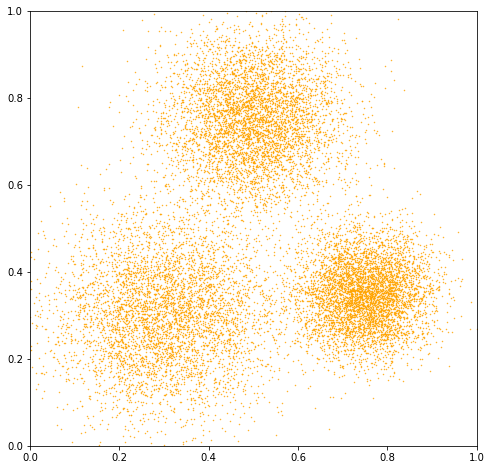
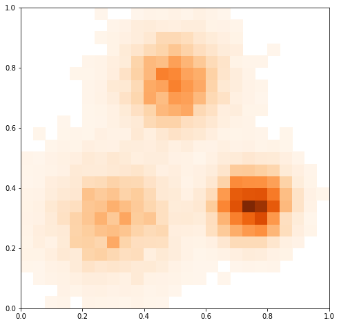
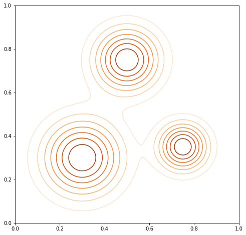
Figure 1: The same distribution defined on $\mathbb{R}^{2}$ approximated as (left) a points cloud, (center) a 2D histogram, (right) a Gaussian mixture density.

Pointwise comparison of measures.

Once the data and the sought-after models are represented as measures, many ML or imaging problems require to assess their similarity. This comparison is performed using a loss function, such as a distance between measures, so that the smaller the loss is, the closer the two measures are. We usually refer to a divergence when the loss is positive and definite, so that the loss is zero if and only if the two measures are identical. Having a loss satisfying the triangle inequality is a desirable feature, but is not mandatory.

To compare discrete distributions on a fixed grid (i.e. histograms), one can directly rely on usual norms such as the $\ell_{2}$ and the $\ell_{1}$ norms. The $\ell_{1}$ norm is often preferable, because it can be extended to general measures (i.e. not necessarily discrete) to define the Total Variation (TV) norm. A related construction is the relative entropy (also called the Kullback-Leibler/KL divergence), which is fundamental in statistics and ML [kullback1997information] because of its connection to maximum likelihood estimation [white1982maximum, gine2021mathematical] and information geometry [amari2000methods]. Section 2.1 details these two discrepancies (KL and TV) within the more general framework of $\varphi$-divergences.

These $\varphi$-divergences have the advantage of simplicity, since they only perform pointwise comparisons of the measures at each position. This however totally ignores the metric of the underlying space. It makes these divergences incapable of comparing discrete distributions with continuous ones (for instance the KL divergence is always $+\infty$ in these cases). This issue motivates the use of other losses which leverage the underlying metric. Examples of such losses are Maximum Mean Discrepancies [gretton2007kernel] and Optimal Transport distances [villani2003], which are detailed in Sections 2.2 and 2.3. This review focuses on Optimal Transport and its extensions, with an emphasis on their applicability for data sciences.

Leveraging geometry.

Leveraging some underlying distance is crucial to define loss functions taking into account the relative positions of the points in the distributions. This helps to capture the salient features of the problem, since geometrically close samples might share similar properties (such as in domain adaptation [courty2014domain], see Section 2.3). The choice or the design of this distance is thus of primary importance. In some cases, some natural metric is induced by the problem under study, such as for instance Euclidean or geodesic distance when studying some physical process [dukler2019wasserstein, cotar2013density]. In some other favorable cases, expert knowledge can be leveraged to design a metric, which can be for instance an Euclidean distance on some hand-crafted features. A representative example is in single cell genomics, where the cell can be embedded in a gene’s space over which OT can be computed [schiebinger2017reconstruction]. In more complicated setups, such as for images or texts, the metric should be learned in parallel to the resolution of the problem. This “metric learning” setup is still an active area of research [kulis2013metric, mikolov2013efficient], and raises many challenging computational and theoretical questions.

Toward robust loss functions between different spaces.

A key difficulty in these applications to data science is to cope with very noisy datasets, which might contain outliers and missing parts. For instance, in applications to single cell genomics [schiebinger2017reconstruction], the data is sensitive to changes of experimental conditions and cells exhibit complex mass variation patterns due to birth/death phenomena. OT faces difficulties in these cases, and is very sensitive to local variations of mass. This sensitivity to noise is illustrated in Section 3, Figure 4, see also [fatras2021unbalanced, mukherjee2021outlier]. At the heart of this review is the description of a robust extension of OT, which is often referred to as unbalanced OT [liero2015optimal] (abbreviated UOT), because of its ability to cope with “unbalanced” measures, i.e. with different masses. But there is more than simply copying with global variation in the total mass of the measure. Most importantly, UOT is more robust to local mass variations, which includes outliers (which get discarded before operating the transport) and missing parts.

Another limitation of OT is its inability to compare measures defined on two distinct spaces. This is for instance the case when comparing different graphs [petric2019got, vayer2020fused] or in genomics when the measurements are performed using distinct modalities [demetci2021unsupervised]. Section LABEL:sec:gw details a variant of OT called Gromov-Wasserstein (GW) which circumvents this issue, at the expense of solving a much more difficult (in particular non-convex) optimization problem.

Notations.

In what follows we consider a metric space $X$ endowed with a distance $d_{X}$. We assume for the sake of simplicity that $X$ is compact, which makes sense in most applications (extension to non-compact spaces requires some control over the moments of the measures). We denote as $\mathcal{C}(X)$ the space of continuous functions endowed with the supremum norm $\left\|f\right\|_{\infty}\triangleq\max_{x\in X}|f(x)|$ for $f\in\mathcal{C}(X)$. We denote as $\int_{X}f\operatorname{\mathrm{d}}\alpha=\int_{X}f(x)\operatorname{\mathrm{d}}\alpha(x)$ the pairing between functions $f\in\mathcal{C}(X)$ and measures in the dual space $\alpha\in\mathcal{M}(X)$ (so that $\alpha$ can be identified as a linear form). A positive measure $\alpha\in\mathcal{M}^{+}_{1}(X)$ is such that $\int_{X}f\operatorname{\mathrm{d}}\alpha\geq 0$ for all positive functions $f\geq 0$. A probability measure, denoted $\alpha\in\mathcal{M}^{+}_{1}(X)$, satisfies the additional property $\alpha(X)=\int_{X}\operatorname{\mathrm{d}}\alpha(x)=1$. For a generic measure $\alpha\in\mathcal{M}^{+}(X)$, the support is defined as the smallest closed set $\operatorname{spt}(\alpha)\subset X$ such that $\alpha(X\setminus\operatorname{spt}(\alpha))=0$.

The strong topology on $\mathcal{M}(X)$ is the dual of the $\left\|\cdot\right\|_{\infty}$ topology on $\mathcal{C}(X)$ and is metrized by the total variation norm (see Section 2.1). The weak${}^{*}$ topology, often referred to as the convergence in law in the case of probability distributions, is – as its name suggests – much weaker and is in some sense a geometric notion of convergence. A sequence $(\alpha_{n})_{n}$ of measures converges weak${}^{*}$ to $\alpha$, denoted $\alpha_{n}\rightharpoonup\alpha$ if and only if for any test function $f\in\mathcal{C}(X)$, one has $\int_{X}f\operatorname{\mathrm{d}}\alpha_{n}\rightarrow\int_{X}f\operatorname{\mathrm{d}}\alpha$. In other terms, it is the pointwise convergence on $\mathcal{C}(X)$ of a sequence of linear forms $(\alpha_{n})_{n}\in\mathcal{M}(X)$. As detailed in Section 2, OT distances and kernel norms metrize this weak${}^{*}$ topology.

We consider in what follows “cost functions” $\text{{C}}:X^{2}\rightarrow\mathbb{R}$, which are assumed to be symmetric ($\text{{C}}(x,y)=\text{{C}}(y,x)$), positive ($\text{{C}}(x,y)\geq 0$), definite ($\text{{C}}(x,y)=0\Rightarrow\,x=y$), and continuous (i.e. $(x,y)\mapsto\text{{C}}(x,y)$ is continuous). A typical example is $\text{{C}}(x,y)=d_{X}(x,y)^{p}$ for some exponent $p>0$. We use such cost functions in the definition of OT (see Section 2.3). It represents in the Monge problem the cost of transporting a unit of mass from $x$ to $y$.

2 $\varphi$-divergences, MMD and Optimal Transport

We detail in this section several discrepancies between positive measures or probabilities, namely $\varphi$-divergences, kernel norms (Maximum Mean Discrepancies) and Optimal Transport. We discuss their theoretical and numerical strengths, as well as their shortcomings. Unbalanced OT in Section 3 consists in blending $\varphi$-divergences and Optimal Transport altogether, while kernel norms are connected to the entropic regularization of OT in Section 4.

2.1 $\varphi$-divergences

One of the simplest family of discrepancies between positive measures are Csiszár divergences [csiszar1967information] (also called $\varphi$-divergences). They consist in integrating pointwise comparisons of two positive measures, and are defined below.

Definition 1 ($\varphi$-divergence).

Define an entropy function as a function $\varphi:(0,\infty)\rightarrow[0,+\infty]$ which is convex, positive, lower-semi-continuous function and such that $\varphi(1)=0$. Define its recession constant $\varphi^{\prime}_{\infty}\triangleq\lim_{p\rightarrow\infty}\varphi(p)/p$. For any $(\alpha,\beta)\in\mathcal{M}^{+}(X)$, write the Radon-Nikodym-Lebesgue decomposition as $\alpha=\tfrac{\operatorname{\mathrm{d}}\alpha}{\operatorname{\mathrm{d}}\beta}\beta+\alpha^{\bot}$. The $\varphi$-divergence is defined as

$$\text{{D}}_{\varphi}(\alpha|\beta)\triangleq\int_{X}\varphi\big{(}\tfrac{\operatorname{\mathrm{d}}\alpha}{\operatorname{\mathrm{d}}\beta}(x)\big{)}\operatorname{\mathrm{d}}\beta(x)+\varphi^{\prime}_{\infty}\int_{X}\operatorname{\mathrm{d}}\alpha^{\bot}(x).$$

Two popular instances of $\varphi$-divergences are the Kullback-Leibler divergence where $\varphi(p)=p\log p-p+1$ (and $\varphi^{\prime}_{\infty}=+\infty$) or the Total Variation divergence $\varphi(p)=|p-1|$ (and $\varphi^{\prime}_{\infty}=1$). See also Section LABEL:sec:exmpl-phidiv for other examples. The former reads

$$\mathrm{KL}(\alpha|\beta)\triangleq\int_{X}\log\big{(}\tfrac{\operatorname{\mathrm{d}}\alpha}{\operatorname{\mathrm{d}}\beta}(x)\big{)}\operatorname{\mathrm{d}}\alpha(x)-\int_{X}\operatorname{\mathrm{d}}\beta+\int_{X}\operatorname{\mathrm{d}}\alpha,$$ (1)

when $\alpha^{\bot}=0$ (which corresponds to $\alpha$ as being absolutely continuous with respect to $\beta$, and is noted $\alpha\ll\beta$), and $\mathrm{KL}(\alpha|\beta)=+\infty$ otherwise. The total variation is a norm and reads

$$\mathrm{TV}(\alpha|\beta)\triangleq\int_{X}|\tfrac{\operatorname{\mathrm{d}}\alpha}{\operatorname{\mathrm{d}}\beta}(x)-1|\operatorname{\mathrm{d}}\beta(x)+\int_{X}\operatorname{\mathrm{d}}\alpha^{\bot}=|\alpha-\beta|(X).$$

Total Variation admits another formulation as the dual norm of $\left\|\cdot\right\|_{\infty}$ (it is an example of an integral probability metric [muller1997integral]). It reads

$$\mathrm{TV}(\alpha|\beta)=\sup_{\left\|f\right\|_{\infty}\leq 1}\int_{X}f\operatorname{\mathrm{d}}(\alpha-\beta),$$

so that TV induces the dual topology induced by the strong topology on $\mathcal{C}(X)$. Thus $\mathrm{TV}$, and more generally Csiszár divergences with $\varphi^{-1}(\{0\})=\{1\}$ (see [liero2015optimal, Corollary 2.9]), induce a stronger topology than the weak${}^{*}$ convergence, i.e. $\text{{D}}_{\varphi}(\alpha_{n}|\alpha)\rightarrow 0$ implies $\alpha_{n}\rightharpoonup\alpha$, but the converse does not hold. For instance take $x_{n}\rightarrow y$ but $x_{n}\neq y$, one has $\delta_{x_{n}}\rightharpoonup\delta_{y}$, but $\mathrm{KL}(\delta_{x_{n}}|\delta_{y})=+\infty$ and $\mathrm{TV}(\delta_{x_{n}}|\delta_{y})=2$. Csiszár divergences integrate pointwise comparison of measures $\tfrac{\operatorname{\mathrm{d}}\alpha}{\operatorname{\mathrm{d}}\beta}(x)$ at any $x\in X$, but ignore the proximity between positions $(x,y)$, hence their incapacity to metrize the weak${}^{*}$ topology.

A chief advantage of these divergences is that they can be computed in $O(N)$ operations for discrete measures $\alpha=\sum_{i}^{N}\alpha_{i}\delta_{x_{i}}$ and $\beta=\sum_{i}^{N}\beta_{i}\delta_{x_{i}}$ sharing the same support $(x_{i})_{i}$, since one has

$$\text{{D}}_{\varphi}(\alpha|\beta)=\sum_{\beta_{i}>0}\varphi\big{(}\tfrac{\alpha_{i}}{\beta_{i}}\big{)}\beta_{i}+\varphi^{\prime}_{\infty}\sum_{\beta_{i}=0}\alpha_{i}.$$

Applications.

As mentioned previously, the KL divergence is at the heart of several statistical methods such as logistic regression [james2013introduction] and maximum-likelihood (ML) estimation [white1982maximum] to fit parametric models of measures. Given an empirical measure $\alpha_{N}=\tfrac{1}{N}\sum_{i=1}^{N}\delta_{x_{i}}$, the maximum-likelihood method aims at finding a parameterized probability distribution $\beta_{\theta}$ approximating $\alpha_{N}$. The key hypothesis is that $\beta_{\theta}$ has a density $\xi_{\theta}$ with respect to some fixed reference measure $\mu$, i.e. $\operatorname{\mathrm{d}}\beta_{\theta}=\xi_{\theta}\operatorname{\mathrm{d}}\mu$ on $X$. The model is estimated on the data support as $\hat{\beta}_{\theta}=\sum_{i=1}^{N}\xi_{\theta}(x_{i})\delta_{x_{i}}$. Maximizing the likelihood is equivalent to minimizing $\theta\mapsto\mathrm{KL}(\alpha_{N}|\hat{\beta}_{\theta})$ with respect to the parameter $\theta$. Logistic regression or Gaussian mixture models [reynolds2009gaussian] correspond to the above minimization problem with a particular choice of the density $\xi_{\theta}$. These minimization problems are often challenging because of the non-convexity w.r.t $\theta$. A standard algorithm is the expectation-maximization (EM) algorithm [moon1996expectation], which is sensitive to the initialization and can be trapped in local minima.

The KL divergence is also at the heart of information geometry [amari2000methods], which is an alternative way to define distances between distributions using Riemannian geometry. It consists in defining a canonical Riemannian manifold structure on a parametric family $(\beta_{\theta})_{\theta}$ of distributions. In the case of distributions with parameters $\theta\in\mathbb{R}^{d}$, if all $\beta_{\theta}$ have a density $\xi_{\theta}$ with respect to a fixed reference measure, then the Riemannian metric is the second order Taylor expansion at $0$ of the function $\delta\theta\mapsto\mathrm{KL}(\beta_{\theta}|\beta_{\theta+\delta\theta})$ w.r.t. $\delta\theta$. The second order term is called the Fisher information matrix and reads

$$g(\theta)\triangleq\int_{X}\big{[}\nabla\log\xi_{\theta}(x)\nabla\log\xi_{\theta}(x)^{\top}\big{]}\operatorname{\mathrm{d}}\beta_{\theta}(x)\in\mathbb{R}^{d\times d}.$$

This matrix defines a quadratic form which in turn induces a geodesic distance. It can be used to perform Riemannian optimization (to solve parameter estimation problems within this family) using for instance the “natural” gradient, which is the gradient with respect to this metric. In general, this metric is difficult to compute, but in some simple cases, closed forms have been derived. For instance, for a Gaussian distribution in $\mathbb{R}$, with covariance $\sigma^{2}$ and mean $m\in\mathbb{R}$, so that $\theta=(m,\sigma)\in\mathbb{R}^{2}$, the Fisher matrix is $g(\theta)=\tfrac{1}{\sigma^{2}}\operatorname{diag}(\tfrac{1}{2},1)$. This Riemannian metric is known as the hyperbolic Poincaré model [cannon1997hyperbolic].

Challenges.

ML estimation enjoys many desirable features, such as providing optimal parameter selection processes in some cases. However, the optimal ML estimator might fail to exist (such as for instance when estimating Gaussian mixtures [lin2004degenerate]), and the model might even fail to have a density with respect to a fixed reference measure, or equivalently, the KL divergence between the data and the model is $+\infty$. A typical example is when training generative learning models [goodfellow2014generative], which correspond to models of the form $\beta_{\theta}=(h_{\theta})_{\sharp}\beta_{0}$, where $(h_{\theta})_{\sharp}$ denotes the push-forward by some parameterized map $h_{\theta}$, and $\beta_{0}$ is a low-dimensional distribution. In this case, the measures $\beta_{\theta}$ are singular, typically supported on low-dimensional manifolds. For these applications, the KL loss should be replaced by weaker losses, which is an important motivation to study geometrically aware losses as we detail next.

2.2 Maximum mean discrepancies

Euclidean norms over a space of measures are defined by integrating so-called kernel functions between the input distributions. They define weaker discrepancies which take into account the underlying distance over $X$.

Reproducing kernels.

A symmetric function $k:X\times X\rightarrow\mathbb{R}$ is called a positive definite (p.d.) kernel on $X$ if for any $n\in\mathbb{N}$, for any $(x_{1},\ldots,x_{n})\in X^{n}$ and $(c_{1},\ldots,c_{n})\in\mathbb{R}^{n}$ one has $\sum_{i,j=1}^{n}c_{i}c_{j}k(x_{i},x_{j})\geq 0$. It is said to be conditionally positive if the above inequality only holds for scalars $(c_{1},\ldots,c_{n})\in\mathbb{R}^{n}$ such that $\sum_{i=1}^{n}c_{i}=0$. In practice the points $(x_{1},\ldots,x_{N})$ correspond to the dataset’s samples, and computing the matrix $K\triangleq(k(x_{i},x_{j}))_{ij}$ is the building block at the basis of all numerical kernel methods. The kernel is called reproducing if there exists a Hilbert space $\mathcal{H}$ of functions from $X$ to $\mathbb{R}$ (with inner product $\langle\cdot,\,\cdot\rangle_{\mathcal{H}}$) such that: (i) for any $x\in X$, $k(\cdot,x)\in\mathcal{H}$ and (ii) for any $x\in X$, for any $f\in\mathcal{H}$, one has $\langle f,\,k(\cdot,x)\rangle_{\mathcal{H}}=f(x)$. The Moore-Aronsazjn Theorem [aronszajn1950theory] states that for any p.d. kernel there exists a unique Hilbert space $\mathcal{H}$ of functions from $X$ to $\mathbb{R}$ such that $k$ is a reproducing kernel. For any reproducing kernel we denote $\psi(x)=k(x,\cdot)$, so that $\psi:X\rightarrow\mathcal{H}$ defines a so-called feature map satisfying $k(x,y)=\langle\psi(x),\,\psi(y)\rangle_{\mathcal{H}}$.

Kernel norms for measures.

The dual norm associated with $\mathcal{H}$ induces the so-called MMD norm on the space of Radon measures since they belong by hypothesis to the dual space of $\mathcal{H}$ [micchelli2006universal, gretton2012kernel].

Definition 2 (MMD norms).

The MMD norm is defined for any $\alpha\in\mathcal{M}^{+}(X)$ as

$$\left\|\alpha\right\|_{\mathcal{H}^{*}}\triangleq\sup_{\left\|f\right\|_{\mathcal{H}}\leq 1}\int_{X}f\operatorname{\mathrm{d}}\alpha.$$

This supremum is reached with a function $f$ which is proportional to $k\star\alpha\triangleq\int_{X}k(\cdot,y)\operatorname{\mathrm{d}}\alpha(y)$ with $\left\|f\right\|_{\mathcal{H}}=1$, so that

$$\left\|\alpha\right\|^{2}_{\mathcal{H}^{*}}=\int_{X^{2}}k(x,y)\operatorname{\mathrm{d}}\alpha(x)\operatorname{\mathrm{d}}\alpha(y).$$ (2)

This norm endows $\mathcal{M}^{+}(X)$ with a Hilbert structure. Thanks to the previous formula, the inner product on $\mathcal{M}^{+}(X)$ reads

$$\langle\alpha,\,\beta\rangle_{\mathcal{H}^{*}}=\int_{X^{2}}k(x,y)\operatorname{\mathrm{d}}\alpha(x)\operatorname{\mathrm{d}}\beta(y).$$

When the pseudo-norm $\left\|\alpha\right\|_{\mathcal{H}^{*}}$ is a norm over the space of measures $\mathcal{M}(X)$, the kernel is said to be definite. When it is a norm only when restricted to measures of total mass $0$, it is said to be conditionally definite. This means that if the kernel is definite (such as the Gaussian kernel), then the associated MMD norm is “unbalanced” and can be used to compare measures with different total mass. It is known to metrize the weak* topology when the kernel is universal, i.e. when the set of functions $\{x\mapsto k(x,y),y\in X\}$ is dense in $\mathcal{C}(X)$ [micchelli2006universal, sriperumbudur2010relation]. On $X=\mathbb{R}^{d}$, typical examples of universal kernels are the Gaussian and Laplacian kernels, of the form $k(x,y)=e^{-\left\|x-y\right\|^{p}/s}$ for respectively $p=2$ and $p=1$, and $s>0$. In contrast, the energy distance kernel $k(x,y)=-\left\|x-y\right\|_{2}$ is universal but only conditionally positive, so it can only be used to compare probability distributions (it is a “balanced” norm).

Applications.

Many machine learning methods such as classification via support vector machines or regression [scholkopf2002learning], statistical tests [gretton2007kernel, gretton2012kernel], or generative learning [li2017mmd, bellemare2017cramer] can be adapted to the setting of reproducing kernel Hilbert spaces. Through the design of adapted kernels, this enables the application of these methods to non-Euclidean data such as strings, sequences and graphs [scholkopf2004kernel]. A typical application is the modeling and classification of proteins [borgwardt2005protein] using graph kernels [bishop2006pattern]. The MMDs leverage these existing kernel constructions to compare collections of points (point clouds) or more generally distributions representing data [gretton2007kernel, gretton2012kernel]. In practice, one usually considers discrete empirical distributions, $(\alpha_{N},\beta_{N})$, often assumed to be drawn from some unknown measures $(\alpha,\beta)$. This is at the heart of two-sample tests to check whether $\alpha=\beta$ by checking if $\left\|\alpha_{N}-\beta_{N}\right\|_{\mathcal{H}^{*}}$ is small enough. Another application of kernels is to perform density estimation [terrell1992variable] by smoothing a discrete measure $\alpha_{N}$ to obtain $(k\star\alpha_{N})(x)\triangleq\int k(x,y)\operatorname{\mathrm{d}}\alpha_{N}(y)$. When $\alpha_{N}=\sum_{i}\alpha_{i}\delta_{x_{i}}$, this smoothing reads $(k\star\alpha_{N})(x)=\sum_{i}\alpha_{i}k(x,x_{i})$.

Numerical computation.

The computation of the MMD norm of some measure $\alpha_{N}=\sum_{i}\alpha_{i}\delta_{x_{i}}$ with $N$ samples requires $N^{2}$ operations, since

$$\left\|\alpha_{N}\right\|_{\mathcal{H}^{*}}^{2}=\sum_{i,j}k(x_{i},x_{k})\alpha_{i}\alpha_{j}=\langle K\alpha,\,\alpha\rangle_{\mathbb{R}^{N}}$$ (3)

where $K\triangleq(k(x_{i},x_{j}))_{i,j}\in\mathbb{R}^{N\times N}$. This might be prohibitive for large datasets, but this complexity can be mitigated using GPU computations [feydy2020fast] and low rank Nyström methods [williams2000using, rudi2017falkon, meanti2020kernel].

An important feature of these MMD norms, compared to OT distances (see Section LABEL:sec:sample-comp) is that they suffer less from the curse of dimensionality [sriperumbudur2012empirical, rudi2017generalization]. The intuition is that the discrete formula (3) is similar to a Monte-Carlo integration technique to approximate (2). If the $(x_{i})_{i}$ are drawn independently from $\alpha$, this explains why the discretization error is of the order $1/\sqrt{N}$, and the decay with $N$ is independent of the dimension.

Challenges.

In practice, the choice of the kernel function has a significant impact on the performance in applications. For instance, the Gaussian kernel $k(x,y)=e^{-\left\|x-y\right\|^{2}/2\sigma^{2}}$ depends on a bandwidth parameter $\sigma$. As illustrated in Figure 2, a poor tuning of $\sigma$ yields a kernel norm which is highly non-convex with respect to shifts of the measures’ supports. By comparison, the energy distance kernel $k(x,y)=-\left\|x-y\right\|_{2}$ is parameter free, and yields a convex loss for this example, but can only be used between probability distributions (and not arbitrary positive measures).

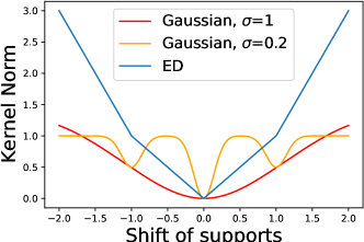
Figure 2: Computation of $\left\|\alpha-\alpha_{\tau}\right\|_{\mathcal{M}^{+}(X)}^{2}$ where $X=\mathbb{R}$, $\alpha=\tfrac{1}{2}\delta_{-0.5}+\tfrac{1}{2}\delta_{0.5}$ and $\alpha_{\tau}=\tfrac{1}{2}\delta_{\tau-0.5}+\tfrac{1}{2}\delta_{\tau+0.5}$. The plot displays the kernel norm value as a function of $\tau\in[-2,2]$. We consider the Gaussian kernel (with $\sigma\in\{0.2,\,1\}$) and the energy distance (ED) kernel.

This non-convexity can be detrimental when using these kernel loss functions to fit models by distance minimization, as in Figure 3. We consider two discrete distributions $\alpha_{x}=\tfrac{1}{N}\sum_{i=1}^{N}\delta_{x_{i}}$ and $\beta_{y}=\tfrac{1}{N}\sum_{i=1}^{N}\delta_{y_{i}}$. We optimize $\alpha_{x}$, which is directly parameterized by the positions $x=(x_{1},\ldots,x_{N})$, by doing a gradient descent of the energy $x\mapsto\mathcal{F}(x)\triangleq\left\|\alpha-\beta\right\|_{\mathcal{H}^{*}}^{2}$. This type of optimization is motivated by applications as diverse as the training of neural networks with a single hidden layer [chizat2018global, rotskoff2019global] (where the $x_{i}$ represent the hidden neurons), domain adaptation [courty2014domain] and optical flow estimation [menze2015object, liu2019flownet3d]. We display in Figure 3 the initialization and the output of the gradient flow after performing gradient descent on $\mathcal{F}(x)$. One sees that for the Gaussian kernel (with small $\sigma$), the output $\alpha$ does not match $\beta$, with even particles moving away from the target $\beta$. For this task the Gaussian kernel is thus not efficient. In contrast, the energy distance kernel is able to retrieve the support of $\beta$, but the convergence is slow and particles are lagging behind. This lag is problematic in training as it requires more gradient descent iterations (and thus it takes more time) to obtain the model’s convergence. Our observations are only empirical and this kernel is not known to have better (Wasserstein) geodesic convexity than Gaussian kernels. Leveraging OT, we show in Section 2.3 it is possible to avoid this issue (see Figure LABEL:fig:flow-reg), thus making it a powerful tool for model fitting tasks.

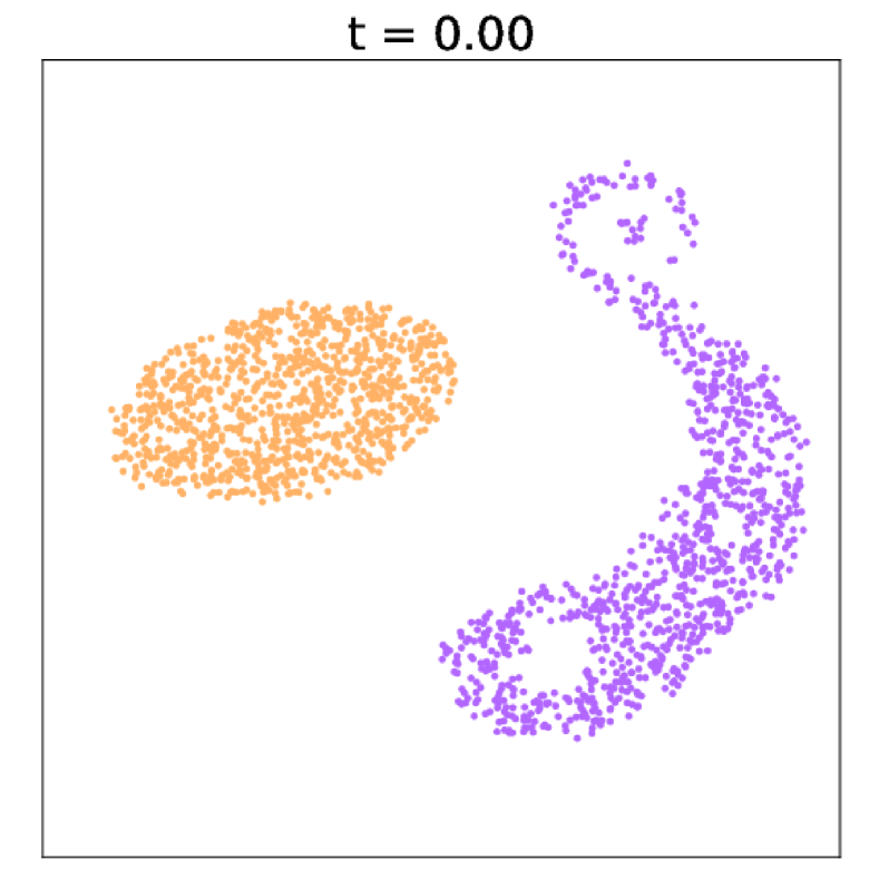
(a) $\alpha(x_{0})$ (orange) and $\beta$ (purple)

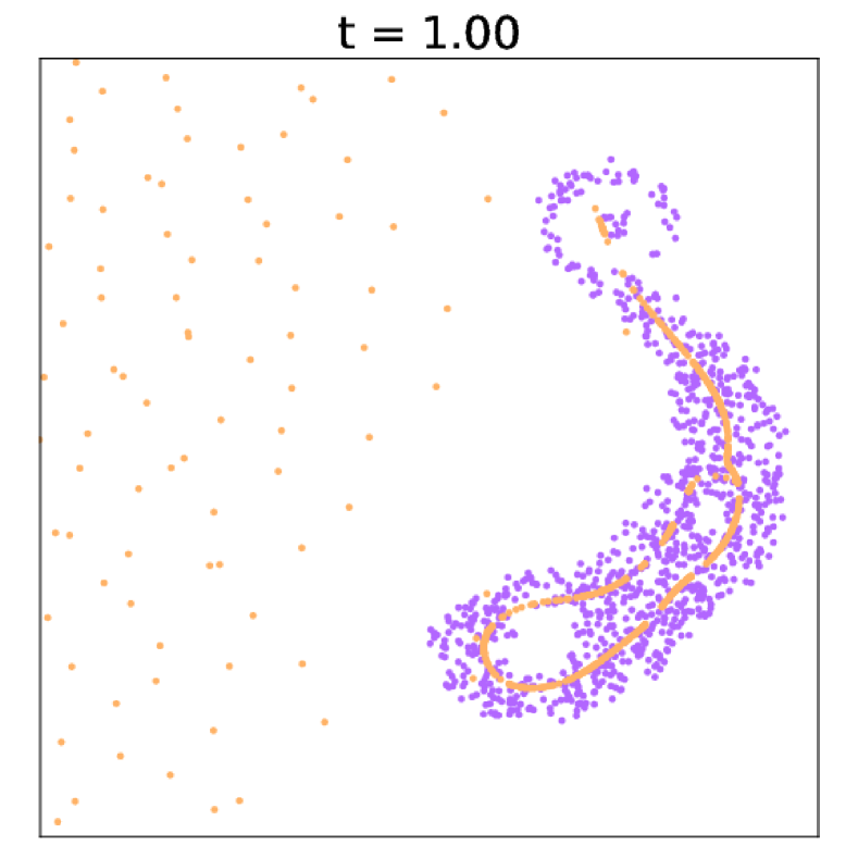
(b) Gaussian kernel

(c) ED kernel

Figure 3: Display of initialization 3(a) and outputs of the gradient flow for the Gaussian kernel 3(b) and the energy distance (ED) kernel 3(c).

Besides fitting distributions, another important use case of OT is to compute “averages” (or barycenters) of several input distributions. A barycenter of $K$ measures $(\alpha_{1},\ldots,\alpha_{K})$ for some discrepancy $\mathcal{L}$ is defined as the minimizer

$$\beta^{\star}=\arg\min_{\beta}\sum_{k=1}^{K}\omega_{k}\mathcal{L}(\beta,\alpha_{k})\quad\text{where}\quad\omega_{k}\geq 0,\;\sum_{k=1}^{K}\omega_{k}=1.$$

Since kernel norms induce a Hilbertian geometry on $\mathcal{M}^{+}(X)$, when $\mathcal{L}(\alpha,\beta)=\left\|\alpha-\beta\right\|^{2}_{\mathcal{H}^{*}}$, the barycenter is simply a linear mixture $\beta^{\star}=\sum_{k=1}^{K}\omega_{k}\alpha_{k}$. In particular, the interpolation between $(\delta_{x},\delta_{y})$ with $\omega=(t,1-t)$ for $t\in[0,1]$ is $\beta^{\star}=t\delta_{x}+(1-t)\delta_{y}$. However, in some applications such as template matching for shapes [bazeille2019local], one might be interested by an interpolation acting on the support instead of the weights, i.e. which reads $\beta^{\star}=\delta_{tx+(1-t)y}$. Doing so requires the use of a non-Hilbertian distance. As we explain in the next section, such interpolation is made possible using Optimal Transport distances (see Figure 5 later in Section 3).

2.3 Balanced Optimal Transport

We provide in this section a brief review on the main properties of Optimal Transport which are useful to the understanding of its unbalanced extension. We refer to the monographs [peyre2019computational, santambrogio2015optimal] for the reader seeking additional numerical illustrations or a deeper analysis of its properties. We recall that for the sake of simplicity, we assume the domain $X$ to be compact.

Monge’s transport.

Optimal Transport (OT) is a problem which traces back to the work of Gaspard Monge [monge1781memoire]. Monge’s problem seeks a matching between two measures $(\alpha,\beta)$ to dig trenches modeled as distributions of sand. Such a map $T:X\rightarrow X$ is constrained to send the mass of $\alpha$ onto $\beta$. This constraint reads $T_{\sharp}\alpha=\beta$, where $T_{\sharp}$ is the push-forward operator defined by the relations $\int_{X}f\circ T\operatorname{\mathrm{d}}\alpha=\int_{X}f\operatorname{\mathrm{d}}\beta$ for any test function $f\in\mathcal{C}(X)$. In particular, this ensures that $T_{\sharp}\delta_{x}=\delta_{T(x)}$. Among all these admissible maps, the optimal transport minimizes the overall cost of transportation, where one assumes some price $\text{{C}}(x,y)$ is associated with a matching $y=T(x)$. A typical example is $\text{{C}}(x,y)=\left\|x-y\right\|_{2}^{p}$ in $X=\mathbb{R}^{d}$ for some $p>0$ (Monge original problem corresponding to $p=1$, while the case $p=2$ enjoys several additional mathematical properties as detailed next).

Definition 3 (OT, Monge formulation).

The optimal transport Monge map, when it exists, solves

$$\inf_{T_{\sharp}\alpha=\beta}\int_{X}\text{{C}}(x,T(x))\operatorname{\mathrm{d}}\alpha(x).$$

OT maps find numerous applications, for instance in domain adaptation [courty2014domain] to extend a trained prediction model from one dataset to another one, or in genomics [demetci2020gromov] to align different pools of cells over some genes’ spaces.

An important question is to check whether such an optimal map exists. If $\alpha$ is discrete but not $\beta$, then no Monge map exists, since $T_{\sharp}\alpha$ is necessarily discrete, so that the mass conservation constraint set $T_{\sharp}\alpha=\beta$ is empty. Brenier’s theorem [brenier1991polar] ensures the existence and uniqueness of a Monge map in $\mathbb{R}^{d}$, for the cost $\text{{C}}(x,y)=\left\|x-y\right\|^{2}$, if $\alpha$ has a density with respect to Lebesgue’s measure. Furthermore the Monge map is the unique gradient of a convex function satisfying the mass conservation constraint, i.e. $T=\nabla u$ with $u$ a convex function.

Kantorovich’s transport.

To deal with arbitrary measures, it is thus necessary to relax the mass conservation equation and to allow for some form of “mass splitting”. This relaxation was introduced by Kantorovich [kantorovich42transfer], first for applications to economic planification. In this formulation, the map $T$ is replaced by a measure $\pi\in\mathcal{M}^{+}(X\times X)$, called a transport plan . Instead of moving all the mass from a position $x$ to $T(x)$, the measure $\pi$ is allowed to move the mass from $x$ to several destinations. This problem is in some sense a relaxation of Monge’s problem (see [santambrogio2015optimal, Section 1.5]).

Definition 4 (OT, Kantorovitch formulation).

An Optimal Transport plan between two positive measures $(\alpha,\beta)\in\mathcal{M}^{+}(X)$ solves

$$\operatorname{OT}(\alpha,\beta)\triangleq\min_{\pi\in\mathcal{U}(\alpha,\beta)}\int_{X^{2}}\text{{C}}(x,y)\operatorname{\mathrm{d}}\pi(x,y),$$

where the constraint set $\mathcal{U}(\alpha,\beta)$ reads

$$\mathcal{U}(\alpha,\beta)\triangleq\bigg{\{}\pi\in\mathcal{M}^{+}(X\times X),\,(p_{X})_{\sharp}\pi=\alpha,\,(p_{Y})_{\sharp}\pi=\beta\bigg{\}},$$

and $p_{X}$ and $p_{Y}:X\times X\rightarrow X$ are canonical projections defined as

$$p_{X}:(x,y)\mapsto x,\qquad p_{Y}:(x,y)\mapsto y.$$

The coupling encodes the amount of mass transported between positions $x$ and $y$, and in this case one pays a price $\text{{C}}(x,y)$ multiplied by the transported mass. The constraint $(p_{X})_{\sharp}\pi=\alpha$ formally means that one has $\int_{X^{2}}f(x)\operatorname{\mathrm{d}}\pi(x,y)=\int_{X}f(x)\operatorname{\mathrm{d}}\alpha(x)$ for any test function $f\in\mathcal{C}(X)$. Intuitively, it means that the sum of the mass transported from a source position $x$ is equal to the mass of $\alpha$ at $x$. It imposes a transportation performed from a source measure $\alpha$ to a target $\beta$, and such that mass is conserved because $\int\operatorname{\mathrm{d}}\pi=\int\operatorname{\mathrm{d}}\alpha=\int\operatorname{\mathrm{d}}\beta$. Note that the problem is infeasible when $\int\operatorname{\mathrm{d}}\alpha\neq\int\operatorname{\mathrm{d}}\beta$, because $\mathcal{U}(\alpha,\beta)=\emptyset$, thus one has $\operatorname{OT}(\alpha,\beta)=+\infty$.

In sharp contrast to Monge’s problem an optimal solution to Kantorovitch’s problem always exists, but might fail to be unique. In particular, the feasible set is always non empty, because $\alpha\otimes\beta\in\mathcal{U}(\alpha,\beta)\neq\emptyset$, (where $\operatorname{\mathrm{d}}(\alpha\otimes\beta)(x,y)\triangleq\operatorname{\mathrm{d}}\alpha(x)\operatorname{\mathrm{d}}\beta(y)$). In addition to providing access to an optimal coupling $\pi$ between the measure, the cost $\operatorname{OT}(\alpha,\beta)$ of the optimization problem itself is of primary importance. Indeed, if $\text{{C}}(x,y)=d_{X}(x,y)^{p}$ for some $p\geq 1$, then $\operatorname{OT}^{1/p}$ defines the so-called $p$-Wasserstein distance [villani2003]. This Wasserstein distance metrizes, when the underlying space is compact, the weak${}^{*}$ convergence, i.e. $\alpha_{n}\rightharpoonup\alpha$ if and only if $\operatorname{OT}(\alpha_{n},\alpha)\rightarrow 0$. A distinctive feature of this distance, among all possible distances metrizing the weak${}^{*}$ topology (such as MMD norms), is that it exactly “lifts” the ground distance in the sense that $\operatorname{OT}^{1/p}(\delta_{x},\delta_{y})=d_{X}(x,y)$.

Discrete setting.

In many applications in data sciences, the distributions are discrete empirical measures, $\alpha=\sum_{i=1}^{N}\alpha_{i}\delta_{x_{i}}$ and $\beta=\sum_{j=1}^{M}\beta_{j}\delta_{y_{j}}$. In this case the $\operatorname{OT}$ problem becomes a finite dimensional linear program

$$\operatorname{OT}(\alpha,\beta)\triangleq\inf_{\pi\in\mathcal{U}(\alpha,\beta)}\quad\sum_{i=1}^{N}\sum_{j=1}^{M}\text{{C}}(x_{i},y_{j})\pi_{i,j},$$

where the marginal constraints on $\pi$ read

$$\mathcal{U}(\alpha,\beta)\triangleq\bigg{\{}\pi\in(\mathbb{R}_{+})^{N\times M},\,\,\sum_{j}\pi_{ij}=\alpha_{i},\,\,\sum_{i}\pi_{ij}=\beta_{j}\bigg{\}}.$$

In this case, $\mathcal{U}(\alpha,\beta)$ defines a compact polytope. A remarkable setting is when $N=M$ (same number of samples) and $\alpha_{i}=\beta_{j}=\tfrac{1}{N}$ (uniform weights), in which case $\mathcal{U}(\alpha,\beta)$ defines the Birkhoff polytope, whose extremal points are permutation matrices. Since OT is a linear program, we thus have the existence of an optimal $\pi^{\star}$ which is a permutation minimizing the transportation of samples $(x_{i})_{i}$ to match samples $(y_{j})_{j}$. This result is true independently of the cost and it does not extend to the continuous setting without assumptions. Indeed, Brenier’s theorem requires a non-degeneracy (so-called twist) condition on the cost to hold. Yet, it highlights the fact that the OT couplings generalize the notion of optimal matching, and are thus quite different from “closest point” matchings routinely used in many applications. For general input measures (i.e. non uniform weights, or when $N\neq M$), the optimal $\pi^{\star}$ is a sparse assignment matrix with less than $M+N$ non zero entries (see [santambrogio2015optimal, Exercise 41]).

Dynamic formulation.

On the Euclidean space and more generally on Riemannian manifolds, when the cost $c$ is the distance squared denoted $d^{2}$, a dynamic formulation of the Kantorovich’s transport was first introduced in [benamou2000computational]. This so-called Benamou-Brenier formulation consists in the minimization of the kinetic energy of the probability measure under the constraint of the continuity equation. Let us denote $\mu(t,x)$ a time-dependent density on the domain $X$ assumed to be a closed convex domain in $\mathbb{R}^{d}$ or a closed Riemannian manifold. This density follows the continuity equation which reads, for $t\in[0,1]$ and $x\in X$

$$\partial_{t}\mu(t,x)+\nabla\cdot(\mu(t,x)v(t,x))=0\,,$$ (4)

where $\partial_{t}$ denotes the partial derivative w.r.t. time, $\nabla\cdot$ is the divergence w.r.t. a chosen reference volume form and $v:[0,1]\times X\to TX$ is a time-dependent vector field, taking values in the tangent space of $X$ denoted by $TX$. Now, the optimal transport distance between $\mu(0,\cdot)$ and $\mu(1,\cdot)$ for the cost $d^{2}$ can be written as the minimization over $\mu(t,x)$ (with fixed endpoints in time) of the kinetic energy

$$\int|v(t,x)|^{2}d\mu(t,x)\,,$$ (5)

under the constraint (4). Note that this formulation of the problem is a priori more complex since it introduces an additional time variable. Even worse, the initial Kantorovich problem is convex whereas this formulation is not convex. One of the key contribution of Benamou and Brenier is to transform it back to a convex problem via

$$\partial_{t}\mu+\nabla\cdot\omega=0\,,$$ (6)

with $\omega=\mu v$, which is now a measure. This change of variable transforms the kinetic energy which is non-convex in $(\mu,v)$ into a one-homogeneous convex Lagrangian $\frac{1}{2}\frac{\|\omega\|^{2}}{\mu}$. As put forward in [benamou2000computational] this formulation can now be solved numerically with convex optimization algorithms.

Note that it is not always the case that the Kantorovich problem can be re-written in such a dynamic form. Indeed, the cost often cannot be naturally reformulated as a Lagrangian on a space of curves in contrast to the Riemannian distance squared. However, the dynamic formulation presents several advantages such as being more flexible to incorporate physical constraints or to extend the Wasserstein metric to the space of positive Radon measures. As we see in the Section 3.2, deriving metric properties of the unbalanced optimal transport problem follows easily by construction.

Algorithms.

In general, OT maps and couplings cannot be computed in closed form. An exception to this is when $(\alpha,\beta)$ are Gaussians, in which case the optimal plan is an affine map and the Wasserstein$-2$ distance admits a closed form, which is the Bures distance between the covariance matrices [bures1969extension].

Several algorithms solve exactly or approximately the OT problem between two discrete measures. Network flow simplexes [orlin1997polynomial] solve OT for any inputs $(\alpha,\beta)$ in $O(N^{3}\log N)$ time. When measures have the same cardinality $N$ and uniform weights $1/N$, the Hungarian algorithm [kuhn1955hungarian] and the auction algorithm [bertsekas1990auction, bertsekas1992auction] compute the permutation matrix in $O(N^{3})$ time. These methods are efficient for medium scale problems, where typically $N\lesssim 10^{4}$.

Under additional assumptions, specific (and thus more efficient) solvers are available. For univariate data (i.e. $(\alpha,\beta)\in\mathcal{M}^{+}(\mathbb{R})$), if the cost reads $\text{{C}}(x,y)=h(x-y)$ with $h:\mathbb{R}\rightarrow\mathbb{R}_{+}$ convex on $\mathbb{R}_{+}$ [santambrogio2015optimal], optimal maps are increasing functions. In the discrete case, solving OT is thus achieved by sorting the data, which requires $O(N\log(N))$ operations.

In the setting of semi-discrete OT where $\alpha$ has a density and $\beta$ is discrete, and for the cost $\text{{C}}(x,y)=\left\|x-y\right\|^{2}$, the Monge map can be solved by leveraging the structure of this map, which is constant on so-called “Laguerre cells” (which generalizes Voronoi cells by including weights). Fortunately, these cells can be computed in linear time in dimension 2 and 3, which can itself be integrated into a quasi-Newton solver to find the weights of the cells [kitagawa2019convergence]. The Wasserstein-$1$ distance on a graph is equivalent to a min-cost-flow problem [santambrogio2015optimal] which is solvable in $O(N^{2}\log N)$ time by Network simplex algorithms. Solving the dynamic formulation is also a way to address medium to large scale OT problems using proximal splitting methods, see [papadakis2014optimal].

It is also possible to build approximations or alternative distances on top of OT computations. An option is to integrate OT distance along 1-D projection, which corresponds to the so-called sliced-Wasserstein distance [bonneel2015sliced]. Combining 1-D OT maps along the axes defines the Knothe map [santambrogio2015optimal], which is a limit of OT maps for degenerate cost functions, and is related to the subspace detours variation of OT [muzellec2019subspace]. One can also approximate OT between mixtures of Gaussians by leveraging the closed form expression of OT between Gaussians [delon2020wasserstein], which finds applications in texture synthesis [leclaire2022optimal].

Applications.

Some models can be directly re-casted as OT optimization problems. This is typically the case in physical models, such as for instance finding the optimal shape of a light reflector problem [glimm2010rigorous, benamou2020entropic] or reconstructing the early universe from a collection of stars viewed as point masses [frisch2002reconstruction, levy2021fast].

In data sciences, OT distances can be used to perform various learning tasks over histograms (often called “bag of features”), such as image retrieval [rubner2000earth, rabin2008circular]. OT distances are also at the heart of statistical tests [ramdas2017wasserstein, sommerfeld2018inference, hundrieser2022unifying], to check equality of two distributions from their samples, and to check the independence by comparing a joint distribution to the product of the marginals. More advanced uses of OT consist in using it as a loss function for imaging and learning. In supervised learning, the features and the output of the learned function are histograms compared using the OT loss. This can for instance be used for supervised vision tasks [frogner2015learning]. This is also used for graph predictions [vayer2020fused, petric2019got], where the features of all nodes on a graph are aggregated into a distribution in $\mathbb{R}^{d}$, and the OT distance serves to train an embedding of these node distributions modeled via a graph neural network [wu2020comprehensive]. In unsupervised learning, for density fitting, one optimizes some parametric model $\beta_{\theta}$ to fit empirical observations viewed as a discrete measure $\alpha_{N}$. This is achieved by minimizing $\theta\mapsto\operatorname{OT}(\alpha_{N},\beta_{\theta})$. A typical instantiation of this problem is to train a generative model [arjovsky2017wasserstein], in which case the model is of the form $\beta_{\theta}=(h_{\theta})_{\sharp}\beta_{0}$ where $h_{\theta}$ is a deep network and $\beta_{0}$ a fixed reference measure in a low dimensional latent space. For imaging sciences, such as in shape matching (which is similar in spirit to generative model training), the transport map cannot be directly used for registration (because it lacks regularity). Though the OT loss can be used to help the trained diffeomorphic models to avoid local minima of the registration energy  [feydy2017optimal]. Other applications in imaging include inverse problems resolution, such as seismic tomography [metivier2016optimal] where the OT loss tends to reduce the presence of local minimizers when resolving the location of reflecting layers in the ground.

The OT map itself also finds applications, for instance in joint domain adaption or transfer learning [courty2016optimal, courty2017joint], where the goal is to learn in an unsupervised setting the labels of a dataset based on another similar dataset which is labeled. In single-cell biology [schiebinger2017reconstruction], the optimal transport plan interpolates between two observations of a cell population at two successive time-steps. In natural language processing [grave2019unsupervised], the input measure of words represents a language embedded in Euclidean spaces using e.g. word2vec [mikolov2013efficient], and assignments are related to translation processes.

Challenges.

The definition of OT imposes a perfect conservation of mass, so that it can only compare probability measures. While it is tempting to use ad-hoc normalizations to cope with this constraint, using directly this formulation of OT makes it non-robust to noise and local variation of mass. We explain in the following Section 3 a simple workaround leading to an extended version of the classical OT theory. We then address in Section 4 the two other major limitations of OT: its high computational cost and its high sample complexity.

3 Unbalanced Optimal Transport

The main idea to lift this mass conservation restriction is to replace the hard constraint encoded in $\mathcal{U}(\alpha,\beta)$ by a soft penalization, leveraging Csiszàr divergence $\text{{D}}_{\varphi}$ from Section 2.1. As illustrated by Figure 4, this constraint forces OT to transport all samples of input distributions, which is an undesirable feature in the presence of outliers, i.e. irrelevant samples. By comparison, relaxing such constraint as is performed by unbalanced OT (defined below) allows to discard such outliers. We review the existing (often equivalent) ways to achieve this, leading to static, dynamic and conic formulations.

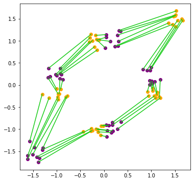
(a) OT matching

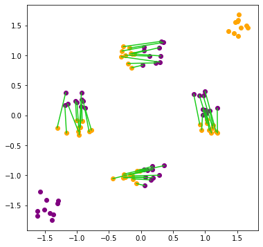
(b) Unbalanced OT matching

Figure 4: Plot of the OT and unbalanced OT matching (in green) between two point clouds $(\alpha,\beta)$ equipped with uniform distributions (in red and blue). Four modes are close to each other, while a fifth mode of each distribution is distant from the rest, and should thus be treated as outlier samples. For OT the matching is forced to make a correspondence between those samples, while for UOT they are indeed discarded. The UOT matching is performed using partial OT [figalli2010optimal], i.e. Definition 5 with $\text{{D}}_{\varphi}=\rho\mathrm{TV}$ and $\rho=0.25$, such that no transport happens when $\text{{C}}\geq 2\rho$.

3.1 Static formulation

As mentioned above, Optimal Transport only has a finite value when the two inputs have the same mass, i.e. $\int_{X}\operatorname{\mathrm{d}}\alpha=\int_{X}\operatorname{\mathrm{d}}\beta$. It is imposed by the constraint set $\mathcal{U}(\alpha,\beta)$ which implies $\int_{X^{2}}\operatorname{\mathrm{d}}\pi=\int_{X}\operatorname{\mathrm{d}}\alpha=\int_{X}\operatorname{\mathrm{d}}\beta$. Thus if this property does not hold, $\mathcal{U}(\alpha,\beta)=\emptyset$ and $\operatorname{OT}(\alpha,\beta)=+\infty$.

In the last few years, several extensions of OT comparing arbitrary positive measures have been developed, based on the different equivalent formulations of OT. The first extensions in the literature focused on the Benamou-Brenier formulation [benamou2000computational], and relax a mass conservation constraint encoded by a continuity PDE [liero2015optimal, liero2016optimal, chizat2018interpolating, kondratyev2016fitness]. This review focuses mostly on the one proposed by [liero2015optimal], which consists in replacing the hard constraints $(p_{X})_{\sharp}\pi=\alpha$ and $(p_{Y})_{\sharp}\pi=\beta$ by $\varphi$-divergences $\text{{D}}_{\varphi_{1}}((p_{X})_{\sharp}\pi|\alpha)$ and $\text{{D}}_{\varphi_{2}}((p_{Y})_{\sharp}\pi|\beta)$ (presented in Section 2.1). It was also proposed in [frogner2015learning] for the particular setting $\text{{D}}_{\varphi}=\mathrm{KL}$. We mainly focus on it because it is convenient from a computational perspective, as we detail in Section 4.1.

Definition 5 (Static unbalanced OT).

The unbalanced OT program optimizes over transport plans $\pi\in\mathcal{M}^{+}(X\times X)$, and reads

$$\operatorname{UOT}(\alpha,\beta)\triangleq\min_{\pi\geq 0}\int_{X^{2}}\text{{C}}(x,y)\operatorname{\mathrm{d}}\pi(x,y)+\text{{D}}_{\varphi_{1}}(\pi_{1}|\alpha)+\text{{D}}_{\varphi_{2}}(\pi_{2}|\beta),$$

where $(\pi_{1},\pi_{2})\triangleq((p_{X})_{\sharp}\pi,(p_{Y})_{\sharp}\pi)$ are the plan’s marginals.

This problem is coined “unbalanced” OT in reference to [benamou2003numerical] who first proposed to relax the marginal constraints for computational purposes. In general $\pi_{1}\neq\alpha$ and $\pi_{2}\neq\beta$. In the UOT problem, the marginals $(\pi_{1},\pi_{2})$ are interpreted as the transported mass, while the ratio of density between e.g. $\pi_{1}$ and $\alpha$ corresponds to the mass which is destroyed and created, i.e. “teleported” instead of being transported.

Note that we retrieve $\operatorname{OT}$ as a particular instance of this problem with $\varphi=\iota_{\{1\}}$ (i.e. $\varphi(1)=0$ and $+\infty$ otherwise), so that $\text{{D}}_{\varphi}=\iota_{(=)}$ satisfies $\iota_{(=)}(\pi_{1}|\alpha)=0$ if $\pi_{1}=\alpha$ and $+\infty$ otherwise. Unbalanced OT is interpretable as a combination of the comparison of masses performed by Csiszár divergences with the comparison of supports operated by OT. Figure 5 illustrates this informal intuition in the setting of barycentric interpolation between two compactly supported parabolic densities in $X=\mathbb{R}$.

It is possible to tune the strength of the mass conservation, i.e. if we prefer to have $\pi_{1}\simeq\alpha$ or allow $\pi_{1}$ to differ significantly from $\alpha$. To do so one can add a parameter $\rho>0$ and use $\text{{D}}_{\rho\varphi}=\rho\text{{D}}_{\varphi}$. One retrieves balanced OT when $\rho\rightarrow\infty$ (provided $\varphi^{-1}(\{0\})=\{1\}$).

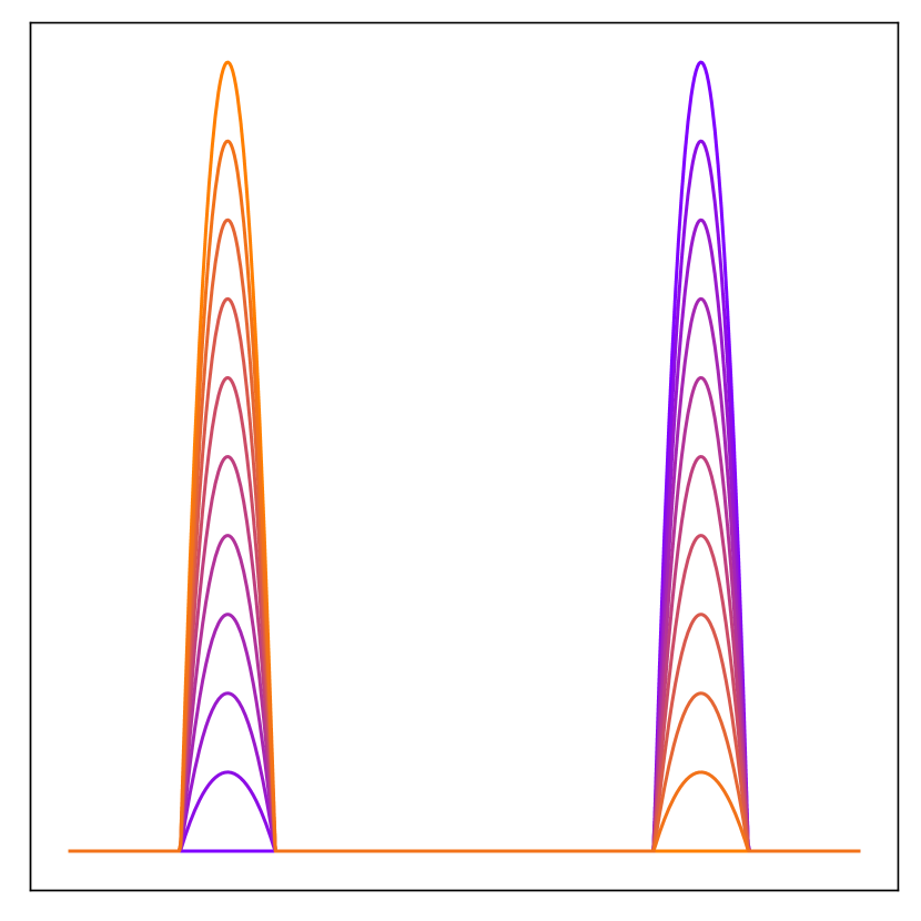
(a) $\mathcal{L}=\text{{D}}_{\varphi}=\mathrm{KL}$

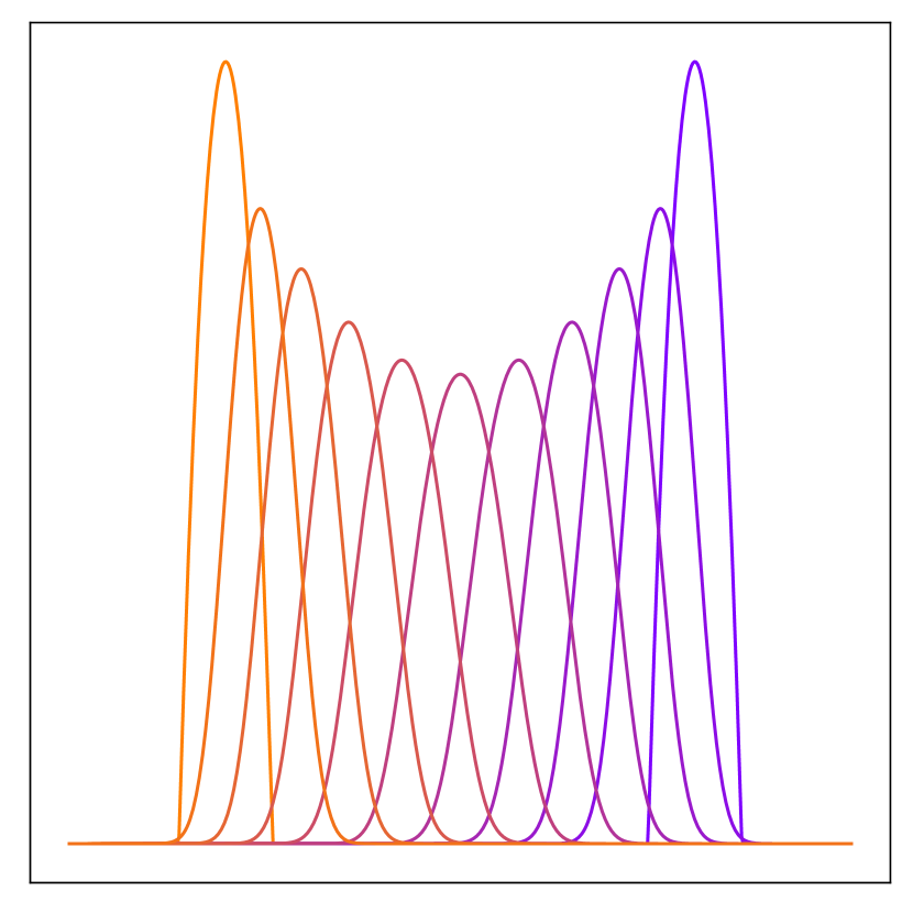
(b) $\mathcal{L}=\operatorname{UOT}$ (same C and $\text{{D}}_{\varphi}$)

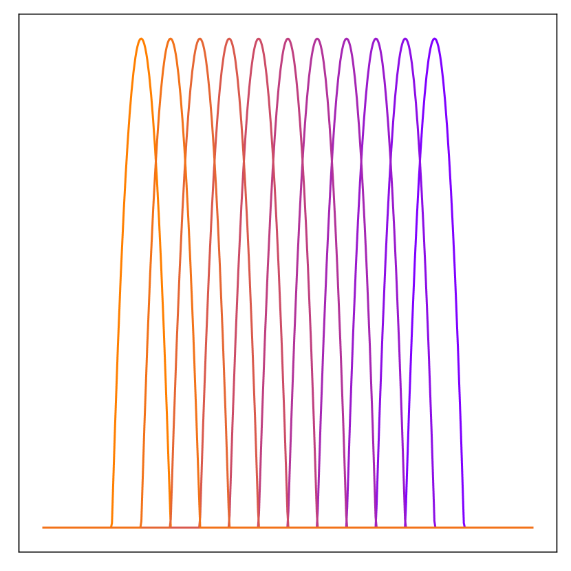
(c) $\mathcal{L}=\operatorname{OT}^{2}$ ($\text{{C}}=\left\|\cdot-\cdot\right\|_{2}^{2}$)

Figure 5: Display of the barycentric interpolation between two (compactly supported) parabolic distributions. It is defined as $\beta^{\star}=\arg\min_{\beta\in\mathcal{M}^{+}_{1}(X)}t\mathcal{L}(\beta,\alpha_{0})+(1-t)\mathcal{L}(\beta,\alpha_{1})$ for $t\in[0,1]$.

Influence of the unbalancedness parameter $\rho$.

Tuning the parameter $\rho$ might be challenging in ML tasks. It corresponds to a characteristic radius of transportation (when $\text{{D}}_{\varphi}=\rho\mathrm{TV}$ there is no transportation if $\text{{C}}_{i,j}>2\rho$), thus its value should be adapted to the cost matrix C. In ML tasks where the cost C is learned or corresponds to a deep feature space, the lack of interpretability complicates the choice of $\rho$, and thus imposes the use of grid-search to tune it.

Figure 6 shows the influence of the relaxation parameter $\rho$ on the optimal plan $\pi$ and on its marginals $(\pi_{1},\pi_{2})$. The computation are done using Sinkhorn’s algorithm detailed in Section 4, which induces a small diffusion (blurring) of the transport plan $\pi$ (the overlaid purple curve shows an approximation of the transport map extracted from this approximated plan). The goal is to highlight the trade-off induced by this parameter selection process, which is crucial for the successful deployment of unbalanced OT in practice. The two inputs $(\alpha,\beta)$ (displayed in dashed lines) are two 1-D mixtures of two Gaussians, but the modes’ amplitudes are not equal. The purpose of this toy example is to illustrate the impact on balanced OT of the mass discrepancy of nearby modes, which forces the optimal transport map to be irregular and to split the mass of each mode. This effect can be seen on the top row, where for $\rho>1$, mass conservation forces the plan $\pi$ to be non-regular. On the contrary, for $\rho<1$, the plan is regular and is locally a translation of the modes, as one should expect.

The middle row shows the evolution of the relaxed marginals $(\pi_{1},\pi_{2})$ as $\rho$ increases. The bottom row gives a quantitative assessment of the evolution: it displays the evolution of the mass of each mode (i.e. on $[0,1/2]$ and $[1/2,1]$). This highlights that as soon as $\rho<1$, neighboring modes have exactly the same mass. This allows the transport plan $\pi$ to match almost exactly the modes using a regular map (almost a translation), which is the desired effect in practice. For $\rho<0.1$, an undesirable effect kicks in: the mass of the marginals becomes too small, and they start to shift from their original location, creating a bias in the transport plan. One can conclude from this numerical analysis that a wide range of $\rho\in[0.1,1]$ leads to a precise estimate of the transportation between the modes of the mixtures, each one being relaxed to modes with constant mass consistent with the original inputs.

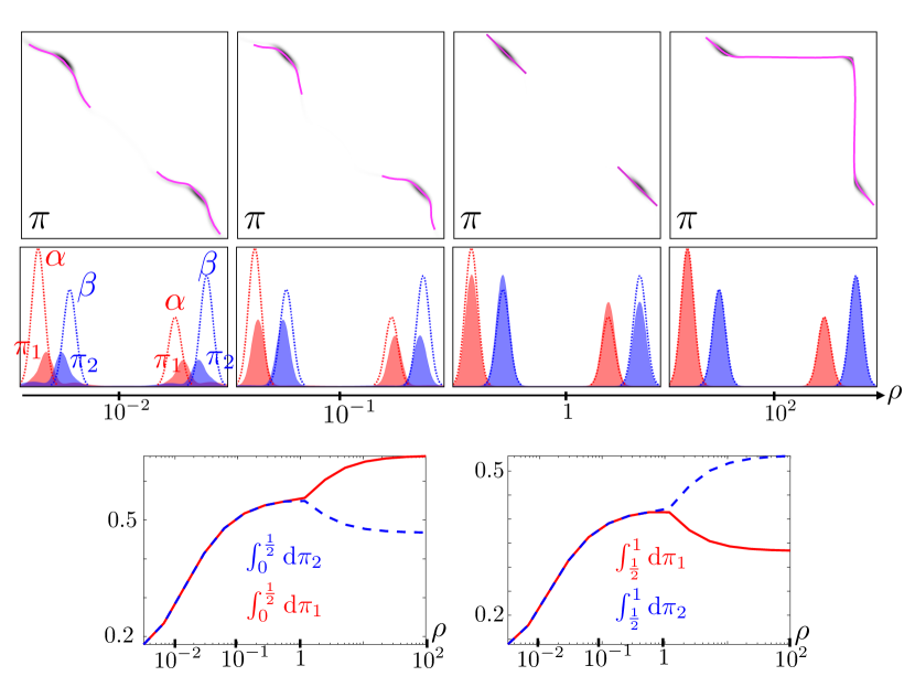
Figure 6: Influence of the relaxation parameter $\rho$ when using $\rho\mathrm{KL}$ relaxation of the marginals’ constraints.

Applications.

Unbalanced OT often improves over the results obtained using balanced OT in most of its application to data sciences. All these examples are also instructive to understand how the parameter $\rho$ should be tuned to reach good performances on large scale datasets. An example in image processing is for video registration using the UOT plan [lee2019parallel]. In shape registration for medical imaging [feydy2019fast], biology [schiebinger2017reconstruction, wu2022metric] and in LiDAR imaging [bevsic2022unsupervised, cattaneo2022lcdnet], UOT is used to provide assignments robust to acquisition noise. UOT can also be used for the theoretical analysis of some statistical and machine learning methods. It is possible to express the gradient descent training of the neurons of a two layers perceptron as a UOT gradient flow, and prove its convergence to global optimality [chizat2018global, rotskoff2019global]. One can also state stability guarantees on the reconstruction of sparse measures in super-resolution problems using UOT [poon2021geometry].

3.2 Dynamic formulation

In this section we present a dynamic formulation of unbalanced optimal transport, based on [chizat2018unbalanced]. This time dependent formulation consists in an optimal control problem on the space of nonnegative Radon measures.

This model is a generalization of the Benamou-Brenier formula presented in the previous section. In order to account for mass change, one considers a continuity equation with a source term. With the notations of the previous section, we introduce

$$\partial_{t}\mu(t,x)+\nabla\cdot(\mu(t,x)v(t,x))=\zeta(t,x)\mu(t,x)\,,$$ (7)

where $\zeta:[0,1]\times X\to\mathbb{R}$ can be understood as a growth rate. One considers a Lagrangian of the type

$$\int_{0}^{1}\int_{X}L(x,v(t,x),\zeta(t,x))\operatorname{\mathrm{d}}\mu(t,x)\,.$$ (8)

Recall that the case of the Benamou-Brenier formula is when $\alpha$ is constrained to be $0$ and $L(x,v)\triangleq\frac{1}{2}\|v\|^{2}$ for the corresponding norm on $TX$. Similarly, this problem has a convex reformulation by introducing

$$\partial_{t}\mu+\nabla\cdot\omega=\xi\,,$$ (9)

with $\omega\triangleq\mu v$ and $\xi\triangleq\zeta\mu$, which are now measures. A quite general setting for dynamic formulations of unbalanced optimal transport is the following minimization problem

$$C_{D}(\alpha,\beta)=\min_{\mu,\omega,\xi}\int_{0}^{1}\int_{X}f\left(x,\frac{\mu}{\lambda},\frac{\omega}{\lambda},\frac{\xi}{\lambda}\right)\operatorname{\mathrm{d}}\lambda(t,x)\,$$ (10)

under the continuity equation constraint (9) and the time-boundary constraints $\mu(t=0,\cdot)=\alpha$ and $\mu(t=1,\cdot)=\beta$. Here, we consider a function $f$ such that $f(x,\cdot,\cdot,\cdot)$ is nonnegative, convex, positively $1-$homogeneous. In comparison with the Lagrangian in Equation (8), we incorporate $\mu$ in the Lagrangian and we impose its $1-$homogeneity. In addition, $\lambda(t,x)$ stands for a measure in time and space dominating all other measures $\mu,\omega$ and $\xi$ and due to the hypothesis on $f$, Definition (10) does not depend on the choice of $\lambda$.

From the continuity equation with a source term, it is clear that simultaneous displacement of mass and change of mass (destruction or creation) is made possible. This is what happens once the optimization has been performed, although the behaviour depends on the chosen Lagrangian. One important example of Lagrangian is, with a little abuse of notations on the variables, $f_{\operatorname{WFR}}(\mu,\omega,\xi)=\frac{1}{2\mu}(\|\omega\|^{2}+\delta^{2}\xi^{2})$ for a positive parameter $\delta$ which leads to the Wasserstein-Fisher-Rao metric, also called Hellinger-Kantorovich. This particular example gives rise to a static formulation with the Kullback-Leibler as the divergence and $c_{\operatorname{WFR}}(x,y)=-\log(\cos^{2}(\min(\frac{1}{2\delta}\|x-y\|,\frac{\pi}{2})))$ as the transportation cost in Definition 5. Another example is $f(\mu,\omega,\xi)=\frac{1}{p}\frac{\|\omega\|^{p}}{\mu^{p-1}}+\delta|\xi|$ for a real parameter $\delta>0$ and it is directly related to partial optimal transport [figalli2010optimal]. In fact, if $(v,g)\mapsto f(x,1,v,g)$ is $p-$positively homogeneous for some $p>1$ and symmetric w.r.t. the origin, then $C_{D}^{1/p}$ is a metric on the space of nonnegative Radon measures.

The main result of this section is that Formulation (10) is equivalent to a static formulation for a cost $c$ that is the convexification of the following cost defined on the cone $X\times\mathbb{R}_{+}$ (see next Section 3.3 for more information on the cone)

$$\tilde{c}((x_{0},m_{0}),(x_{1},m_{1}))=\inf_{x(t),m(t)}\int_{0}^{1}f(x(t),m(t),m(t)x^{\prime}(t),m^{\prime}(t))dt\,,$$ (11)

where the optimization variable is an absolutely continuous path $(x(t),m(t))$ between $(x_{0},m_{0})$ and $(x_{1},m_{1})$. The convexification of $\tilde{c}$ is $c((x_{0},m_{0}),(x_{1},m_{1}))\triangleq\min_{m_{0}^{i},m_{1}^{i}}\tilde{c}((x_{0},m_{0}^{1}),(x_{1},m_{1}^{1}))+\tilde{c}((x_{0},m_{0}^{2}),(x_{1},m_{1}^{2}))$ where $m_{0}^{1}+m_{0}^{2}=m_{0}$ and $m_{1}^{1}+m_{1}^{2}=m_{1}$. We now introduce a static formulation called semi-couplings introduced in [chizat2018global] and used in [bauer2021square] to derive an explicit algorithm. Semi-couplings are couples of nonnegative Radon measures $\gamma,\pi$ on $X\times X$ such that $\gamma_{1}=\alpha$ and $\pi_{2}=\beta$. The static problem is the minimization over the set of semi-couplings of

$$C_{K}(\gamma,\pi)=\inf_{\gamma,\pi}\int_{X\times X}c\left((x,\frac{\gamma}{\lambda}(x,y)),(y,\frac{\pi}{\lambda}(x,y))\right)d\lambda(x,y)\,,$$ (12)

for $\lambda$ any measure dominating $\gamma,\pi$. Again, if for some $p\geq 1$ the cost $c$ is such that $c^{1/p}$ is a distance on the cone then $C_{K}^{1/p}$ is a distance on the space of positive Radon measures on $X$.

Theorem 1.

(Informal, from [chizat2018unbalanced]) The dynamic and the semi-coupling formulations give the same value, i.e. $C_{D}(\alpha,\beta)=C_{K}(\alpha,\beta)$.

We refer to [chizat2018unbalanced] for the dual problem of dynamic and static formulations. Using the dual formulation of the static problem one proves that the semi-coupling formulation has an equivalent UOT formulation. Let us detail the Wasserstein-Fisher-Rao metric case for which $f_{\operatorname{WFR}}$ is defined above. Denoting $C_{\operatorname{WFR}}$ the corresponding dynamic cost, $C_{\operatorname{WFR}}(\alpha,\beta)=2\delta^{2}\operatorname{UOT}(\alpha,\beta)$ in which $\operatorname{UOT}$ is used with the cost $c_{\operatorname{WFR}}$ and the Kullback-Leibler divergences defined in Formula (1). To conclude, we underline that the dynamic cost often gives a length space on the space of positive Radon measures; the most important example being the Wasserstein-Fisher-Rao metric presented above which is an equivalent of the Wasserstein $L^{2}$ metric to the space of positive Radon measure.

3.3 Conic formulation

This section focuses on another formulation of unbalanced OT, which is proved in [liero2015optimal] to be equivalent to the UOT formulation (Definition 5). This second formulation is useful to prove metric properties of UOT. It was adapted to the setting of Gromov-Wasserstein distances to extend it for the unbalanced setting (see Section LABEL:sec:ugw or [sejourne2021unbalanced]).

We detail below the principle of the conic formulation, as well as its derivation to provide understanding on its link with UOT. Then we present its metric properties, and review explicit settings existing in the literature.

Conic lifting.

Informally, this lifting corresponds to map a weighted Dirac mass $r\delta_{x}\in\mathcal{M}^{+}(X)$ to $\delta_{(x,r)}$, where $(x,r)\in X\times\mathbb{R}_{+}$ and $r$ is the particle’s mass. This lifts the space $X$ into $X\times\mathbb{R}_{+}$, more precisely it is lifted onto the cone $\mathfrak{C}[X]\triangleq(X\times\mathbb{R}_{+})/\equiv$, where the equivalence relation on $X\times\mathbb{R}_{+}$ reads $[x,r]\equiv[y,s]\Leftrightarrow(r=s=0)\,\,\text{or}\,(x=y\,\,\text{and}\,\,r=s)$. Note that having $r=s=0$ corresponds to comparing two particles with no mass, thus their positions do not matter and are considered to be equal w.r.t. $\equiv$. Geometrically, such samples are located at the apex of the cone, and the notation $[x,r]\in\mathfrak{C}[X]$ emphasizes the quotient at the apex (compared to $(x,r)\in X\times\mathbb{R}_{+}$). See Figure 7 for an illustrated example of a cone set.

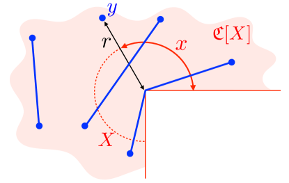
Figure 7: Example of cone $\mathfrak{C}[X]$, where $X$ is a piece of circle whose angles $x$ lie in $[0,\tfrac{3\pi}{2}]$, endowed with the ground (geodesic) distance $d_{X}(x_{1},x_{2})=|x_{1}-x_{2}|$ for $(x_{1},x_{2})\in X$. The cone $\mathfrak{C}[X]$ is represented in red and embedded in $\mathbb{R}^{2}$ via $(y_{1},y_{2})=(r\cos x,r\sin x)$. Three geodesics in $\mathfrak{C}[X]$ are represented in blue. Note the bottom geodesic has a shortest path passing via the cone’s apex.

Lifting positive measures on a cone.

Given a positive measure $\alpha\in\mathcal{M}^{+}(X)$ one can lift it as a measure defined over $\mathfrak{C}[X]$ (i.e. in $\mathcal{M}^{+}(\mathfrak{C}[X])$). One admissible lift of $\alpha$ is $\mathfrak{p}_{\sharp}(\alpha\otimes\delta_{1})$, where $\mathfrak{p}(x,r)\triangleq[x,r]$ is the canonical injection from $X\times\mathbb{R}_{+}$ to $\mathfrak{C}[X]$. In the case of a Dirac $r\delta_{x}$ this lift is $r\delta_{[x,1]}$. However, more elaborate lifts are possible, and play a key role in the analysis of metric properties. In particular, one can show that it is always possible to lift a positive measure of $\mathcal{M}^{+}(X)$ to a probability distribution in $\mathcal{M}^{+}_{1}(\mathfrak{C}[X])$, in order to re-cast unbalanced OT problems over $\mathcal{M}^{+}(X)$ as balanced OT problems over $\mathcal{M}^{+}_{1}(\mathfrak{C}[X])$, with respect to a new cost $d_{\mathfrak{C}}$ (see [liero2015optimal, Corollary 7.7]).

Deriving the conic formulation - Homogeneous formulation.

We detail in this paragraph how one can reformulate the UOT problem (Definition 5) to connect it with its equivalent conic formulation. This derivation involves an intermediate formulation which we call homogeneous. To the best of our knowledge, this formulation has not yet been considered for applications in the literature. However, it is a key intermediate problem to clarify the equivalence between UOT and the conic formulation.

The derivation consists in decomposing Csiszár entropies $\text{{D}}_{\varphi}$ and refactoring all terms involving $\pi$ as a single integral. To do so we define the reverse entropy as $\psi(r)\triangleq r\varphi(\tfrac{1}{r})$ for $r>0$, $\psi(0)=\varphi^{\prime}_{\infty}$ and $\psi^{\prime}_{\infty}=\varphi(0)$. The reverse entropy is such that $\text{{D}}_{\varphi}(\pi_{1}|\alpha)=\text{{D}}_{\psi}(\alpha|\pi_{1})$. Before rewriting the $\operatorname{UOT}$ formulation, we define the following Lebesgue decompositions of $\alpha$ w.r.t $\pi_{1}$ and $\beta$ w.r.t. $\pi_{2}$, which read

$$\alpha=\xi_{1}\pi_{1}+\alpha^{\bot}\quad\text{and}\quad\beta=\xi_{2}\pi_{2}+\beta^{\bot},$$ (13)

such that e.g.

$$\text{{D}}_{\varphi}(\pi_{1}|\alpha)=\text{{D}}_{\psi}(\alpha|\pi_{1})=\int_{X}\psi\big{(}\xi_{1}(x)\big{)}\operatorname{\mathrm{d}}\pi_{1}(x)+\psi^{\prime}_{\infty}\int_{X}\operatorname{\mathrm{d}}\alpha^{\bot}(x).$$

Write $\mathcal{P}_{0}$ the primal functional of Definition 5. Its reformulation reads

$$\mathcal{P}_{0}(\pi) =\int_{X^{2}}\text{{C}}(x,y)\operatorname{\mathrm{d}}\pi(x,y)+\text{{D}}_{\varphi_{1}}(\pi_{1}|\alpha)+\text{{D}}_{\varphi_{2}}(\pi_{2}|\beta)$$

$$=\int_{X^{2}}[\text{{C}}(x,y)+\psi(\xi_{1}(x))+\psi(\xi_{2}(y))]\operatorname{\mathrm{d}}\pi(x,y)$$

$$\quad+\psi^{\prime}_{\infty}\int\operatorname{\mathrm{d}}\alpha^{\bot}+\psi^{\prime}_{\infty}\int\operatorname{\mathrm{d}}\beta^{\bot}$$

$$=\int L_{\text{{C}}(x,y)}(\xi_{1}(x),\xi_{2}(y))\operatorname{\mathrm{d}}\pi(x,y)$$

$$\quad+\psi^{\prime}_{\infty}(|\alpha^{\bot}|+|\beta^{\bot}|),$$

where $L_{c}(r,s)\triangleq c+\psi(r)+\psi(s)$, $|\alpha^{\bot}|\triangleq\alpha^{\bot}(X)$ and $|\beta^{\bot}|\triangleq\beta^{\bot}(X)$. The above formulation is helpful to explicit the terms of pure mass creation/destruction $(|\alpha^{\bot}|+|\beta^{\bot}|)$, and reinterpret the integral under $\pi$ as a transport term with a new cost $L_{\text{{C}}}$ accounting for partial transport and destruction/creation of mass.

The conic formulation is motivated by a pre-optimization of the plan’s mass, i.e. optimizing over plans $\theta\pi$ where $\theta\in\mathbb{R}_{+}$. The plan $\theta\pi$ has marginals $(\theta\pi_{1},\theta\pi_{2})$, the Lebesgue densities of Equation (13) become $(\tfrac{\xi_{1}}{\theta},\tfrac{\xi_{2}}{\theta})$ and $(\alpha^{\bot},\beta^{\bot})$ are unchanged, which yields

$$\mathcal{P}_{0}(\theta\pi)=\int\theta L_{\text{{C}}(x,y)}(\tfrac{\xi_{1}(x)}{\theta},\tfrac{\xi_{2}(y)}{\theta})\operatorname{\mathrm{d}}\pi(x,y)+\psi^{\prime}_{\infty}(|\alpha^{\bot}|+|\beta^{\bot}|).$$

Note the scaling $\theta$ performs a perspective transformation on the function $L_{\text{{C}}}$.

The homogeneous formulation is obtained by optimizing over scalings $\theta(x,y)$ in $\mathbb{R}_{+}$ the function $L_{\text{{C}}}$ (but not the functional $\mathcal{P}_{0}$). Informally speaking, the mass is rescaled at a local scale (i.e. for any $(x,y)$) instead of globally optimizing the plan’s mass (with a constant $\theta\in\mathbb{R}_{+}$). Define the 1-homogeneous function $H_{c}$ as the perspective transform of $L_{c}$

$$H_{c}(r,s)\triangleq\inf_{\theta\geq 0}\theta\big{(}c+\psi(\tfrac{r}{\theta})+\psi(\tfrac{s}{\theta})\big{)}=\inf_{\theta\geq 0}\theta L_{c}(\tfrac{r}{\theta},\tfrac{s}{\theta}).$$ (14)

The function $H_{c}$ can be computed in closed form for a certain number of common entropies $\varphi$. We detail explicit settings in Section 3.3.1, and we refer to [liero2015optimal, Section 5] for a broader overview. Eventually one defines another formulation called homogeneous. It reads

$$\operatorname{HOT}(\alpha,\beta)\triangleq\underset{\pi\in\mathcal{M}(X^{2})}{\inf} \int H_{\text{{C}}(x,y)}(\xi_{1}(x),\xi_{2}(y))\operatorname{\mathrm{d}}\pi(x,y)$$ (15)

$$+\psi^{\prime}_{\infty}(|\alpha^{\bot}|+|\beta^{\bot}|),$$

The term “homogeneous” stems from the $1$-homogeneity of $H_{\text{{C}}}$ in $(r,s)$. By definition one has $L_{c}\geq H_{c}$, so that $\operatorname{UOT}\geq\operatorname{HOT}$. Thanks to the convexity of these problems one actually has $\operatorname{UOT}=\operatorname{HOT}$ (see [liero2015optimal, Section 5]).

Definition of the conic formulation.

The conic formulation consists in rewriting the program $\operatorname{HOT}$ (Equation (15)) over the cone. Instead of a transport plan $\pi(x,y)\in\mathcal{M}^{+}(X^{2})$, we consider a plan $\eta([x,r],[y,s])\in\mathcal{M}^{+}(\mathfrak{C}[X]^{2})$ matching points defined over the cone. The formulation involves a cone cost $d_{\mathfrak{C}[X]}$ which lifts the cost C over $\mathfrak{C}[X]^{2}$, and is derived from the function $H_{c}$. One replaces the densities $(\xi_{1},\xi_{2})$ by radial coordinates $(r,s)$ in $\operatorname{HOT}$. This change of variables allows to cancel out the term $(|\alpha^{\bot}|+|\beta^{\bot}|)$, and replace it by two conic marginal constraints reminiscent of the set $\mathcal{U}(\alpha,\beta)$ of balanced OT. It yields the following definition of the conic formulation.

Definition 6.

The conic formulation is defined as

$$\operatorname{COT}(\alpha,\beta)\triangleq\min_{\eta\in\mathcal{U}^{\mathfrak{C}}(\alpha,\beta)}\int_{\mathfrak{C}[X]^{2}}d_{\mathfrak{C}[X]}([x,r],[y,s])^{q}\operatorname{\mathrm{d}}\eta([x,r],[y,s]),$$ (16)

where the cone cost $d_{\mathfrak{C}[X]}$ is defined using the function $H_{c}$ (Equation (14)), and involves exponents $(p,q)\in\mathbb{R}_{+}$ (larger than $1$), such that

$$d_{\mathfrak{C}[X]}([x,r],[y,s])^{q}\triangleq H_{\text{{C}}(x,y)}(r^{p},s^{p}),$$ (17)

and where the conic constraints $\mathcal{U}^{\mathfrak{C}}(\alpha,\beta)$ are defined as

$$\left\{\eta\in\mathcal{M}_{+}(\mathfrak{C}[X]^{2})\;:\;\int_{\mathbb{R}_{+}}r^{p}\operatorname{\mathrm{d}}\eta_{1}([\cdot,r])=\alpha,\int_{\mathbb{R}_{+}}s^{p}\operatorname{\mathrm{d}}\eta_{2}([\cdot,s])=\beta\right\}.$$ (18)

Here $\eta_{1},\eta_{2}\in\mathcal{M}^{+}(\mathfrak{C}[X])$ denote the marginals of $\eta$ by integrating over one cone coordinate $[x,r]$ or $[y,s]$. If one takes a test function $\xi\in\mathcal{C}(X)$, the first constraint reads $\int r^{p}\xi(x)\operatorname{\mathrm{d}}\eta_{1}([x,r])=\int\xi(x)\operatorname{\mathrm{d}}\alpha(x)$. The additional constraints on $(\eta_{1},\eta_{2})$ mean that the lift of the mass on the cone must be consistent with the total mass of $(\alpha,\beta)$. We emphasize that the conic lifts satisfy an invariance to some operation called dilations, such that optimal plans can only be unique up to such transformation.

The optimization program defining COT thus consists in minimizing the Wasserstein distance $\operatorname{OT}_{d_{\mathfrak{C}[X]}}(\eta_{1},\eta_{2})$ on the cone $(\mathfrak{C}[X],d_{\mathfrak{C}[X]})$. As we show below, when $d_{\mathfrak{C}[X]}$ is a distance, COT inherits the metric properties of $\operatorname{OT}_{d_{\mathfrak{C}[X]}}$.

Proposition 1 (From [liero2015optimal] and [de2019metric]).

One has $\operatorname{UOT}=\operatorname{COT}$, which are symmetric, positive and definite if $d_{\mathfrak{C}[X]}$ is definite. Furthermore, if $(X,d_{X})$ and $(\mathfrak{C}[X],d_{\mathfrak{C}[X]})$ are metric spaces with $X$ separable, then $\mathcal{M}_{+}(X)$ endowed with $\operatorname{COT}$ is a metric space.

This proposition emphasizes that the metric properties of $d_{\mathfrak{C}[X]}$ are key to obtain metric properties of COT and UOT. We detail explicit settings where it holds in Section 3.3.1.

Computation of COT.

It seems a priori harder to solve this conic problem than the original UOT problem, because of the extra radial coordinates $(r,s)\in\mathbb{R}_{+}$. However it is proved in [liero2016optimal, Proposition 3.9] that among optimal conic plans $\eta^{\star}$ of $\operatorname{COT}(\alpha,\beta)$ (recall from the previous paragraph there is not uniqueness), there exists a plan which can be expressed using the optimal plan $\pi^{\star}$ for $\operatorname{UOT}(\alpha,\beta)$. This optimal plan has a single Dirac along each radial coordinate, i.e. it is such that $\eta^{\star}$-a.e., the radiuses are functions $(r(x),s(y))$ of the ground space variables $(x,y)\in X^{2}$. This means that solving the $\operatorname{COT}$ problem reduces to the computation of a UOT problem followed by a conic lifting.

3.3.1 Examples of cone distances

As highlighted by Proposition 1, the settings where $d_{\mathfrak{C}[X]}$ is a distance on $\mathfrak{C}[X]$ are of particular interest. In this section we write the cost as $\text{{C}}(x,y)=\Omega(d_{X}(x,y))$, where $d_{X}$ is a distance on $X$, so that $\Omega:\mathbb{R}_{+}\rightarrow\mathbb{R}_{+}$ plays the role of a renormalization that transfers metric properties from $X$ to $\mathfrak{C}[X]$. In general $d_{\mathfrak{C}[X]}$ is not a distance, but it is always definite on $\mathfrak{C}[X]$, provided $d_{X}$ is definite on $X$, $\Omega^{-1}(\{0\})=\{0\}$ and $\varphi^{-1}(\{0\})=\{1\}$, as proved in [de2019metric, Theorem 7]. Given its definition (Equation 17), the metric properties depend on the choice of $(\varphi,\Omega,p,q)$. We detail four particular settings where this is the case. In each setting we provide $(\text{{D}}_{\varphi},\Omega,p,q)$ and its associated cone distance $d_{\mathfrak{C}[X]}$.

Gaussian Hellinger distance.

It corresponds to

$$\text{{D}}_{\varphi}=\rho\mathrm{KL},\quad\Omega(t)=t^{2}\quad\text{and}\quad q=p=2,$$

$$d_{\mathfrak{C}[X]}([x,r],[y,s])^{2}=\rho\big{[}r^{2}+s^{2}-2rse^{-d_{X}(x,y)^{2}/2\rho}\big{]},$$

in which case it is proved in [liero2015optimal] that $d_{\mathfrak{C}[X]}$ is a cone distance.

Hellinger-Kantorovich / Wasserstein-Fisher-Rao distance.

It reads

$$\text{{D}}_{\varphi}=\mathrm{KL},\quad\Omega(t)=-\log\cos^{2}(\min(\tfrac{\pi}{2},t))\quad\text{and}\quad q=p=2,$$

$$d_{\mathfrak{C}[X]}([x,r],[y,s])^{2}=r^{2}+s^{2}-2rs\cos(\min(\tfrac{\pi}{2},d_{X}(x,y))),$$

in which case it is proved in [burago2001course] that $d_{\mathfrak{C}[X]}$ is a cone distance. The weight $\Omega(t)=-\log\cos^{2}(\min(\tfrac{\pi}{2},t))$ might seem more peculiar but it arises from the dynamical formulation of section 3.2. The Wasserstein-Fisher-Rao metric is actually the length space induced by the Gaussian-Hellinger distance (if the ground metric $d_{X}$ is itself geodesic), as proved in [liero2016optimal, chizat2018interpolating]. This weight introduces a cut-off, because $\Omega(d_{X}(x,y))=+\infty$ if $d_{X}(x,y)>\pi/2$. There is no transport between points too far from each other. The choice of $\pi/2$ is arbitrary, and can be modified by scaling $t\mapsto\Omega(t/\rho)$ for some cutoff $\rho>0$. Note it differs slightly from taking $\text{{D}}_{\varphi}=\rho\mathrm{KL}$.

Power entropy distance.

The distance induced by $\text{{D}}_{\varphi}=\mathrm{KL}$ is extended in [de2019metric] to power entropies $\text{{D}}_{\varphi}$ with $\varphi(t)=\rho\frac{t^{k}-k(t-1)-1}{k(k-1)}$, where $k\notin\{0,1\}$. The Kullback-Leibler divergence is retrieved when $k=1$. When $\Omega(t)=t^{2}$, $p=1$, $q=2$ and $k>1$, they prove that the induced cone cost $d_{\mathfrak{C}[X]}$ is a metric over $\mathfrak{C}[X]$ which reads

$$d_{\mathfrak{C}[X]}([x,r],[y,s])^{2}=\frac{2\rho}{k}\bigg{[}\frac{r+s}{2}-\big{(}\tfrac{r^{1-k}+s^{1-k}}{2}\big{)}^{\frac{1}{1-k}}\bigg{(}1+(1-k)\tfrac{d_{X}^{2}(x,y)}{2\rho}\bigg{)}_{+}^{\frac{k}{k-1}}\bigg{]}.$$

We refer to [de2019metric] for variants of parameterized power-entropies which define cone metrics. A Sinkhorn algorithm for these entropies is derived in [sejourne2019sinkhorn], see also Section LABEL:sec:exmpl-phidiv.

Partial optimal transport.

It corresponds to

$$\text{{D}}_{\varphi}=\rho\mathrm{TV},\quad\Omega(t)=t^{q}\quad\text{and}\quad q\geq 1\quad\text{and}\quad p=1,$$

$$d_{\mathfrak{C}[X]}([x,r],[y,s])^{q}=\rho\big{[}r+s-\min(r,s)(2-\tfrac{d_{X}(x,y)^{q}}{\rho})_{+}\big{]},$$

in which case it is proved in [chizat2018unbalanced] that $d_{\mathfrak{C}[X]}$ is a cone distance. The case $\text{{D}}_{\varphi}=\mathrm{TV}$ is equivalent to partial unbalanced OT, which produces discontinuities (because of the non-smoothness of the divergence) between regions of the supports which are being transported and regions where mass is being destroyed/created. Note that [liero2015optimal] does not mention that such cone cost $d_{\mathfrak{C}[X]}$ defines a distance, although it can be proved without a conic lifting that partial OT defines a distance as explained in [chizat2018unbalanced].

3.4 Discussion and synthesis on UOT formulations

To conclude this exposition of the various formulations of unbalanced OT, we provide below important remarks on the different formulations, their advantages and shortcomings, as well as their relations.

Relationships.

The conic formulation is more general than the static and the dynamic one. Indeed, as formalized by Equations (14) and (12), for any static and dynamic formulation, one can associate a cone cost and thus a conic formulation. However, one can imagine costs on the cone which are not derived from such settings, hence the broader generality of conic formulations.

The static and the dynamic formulations are not completely equivalent. Dynamic formulations induce geodesic distances, but not all static formulations satisfy this property. Reciprocally, not all dynamic problems can a priori be rephrased as a static one for which the cost is explicit, such as for e.g. a Lagrangian with a term $|\xi|^{p}$ for $p\notin\{1,2\}$. There is however an overlap between the static and the dynamic formulations. The two well-known settings are the Wasserstein-Fisher-Rao/Hellinger-Kantorovich distance and Partial OT. The former has a dynamic Lagrangian $f_{\operatorname{WFR}}(\mu,\omega,\xi)=\frac{1}{2\mu}(\|\omega\|^{2}+\delta^{2}\xi^{2})$, corresponding to the cost $\text{{C}}(x,y)=-\log(\cos^{2}(\min(\frac{1}{2\delta}\|x-y\|,\frac{\pi}{2})))$ and $\text{{D}}_{\varphi}=\mathrm{KL}$. The latter has Lagrangian $f(\mu,\omega,\xi)=\frac{1}{p}\frac{\|\omega\|^{p}}{\mu^{p-1}}+\delta|\xi|$, corresponding to a static setting $\text{{C}}(x,y)=\|x-y\|^{p}/p$ and $\text{{D}}_{\varphi}=\delta\mathrm{TV}$. Recall also that both settings are equivalent to the third conic formulation, see Section 3.3.1 for formulas.

These two settings also share equivalence with other formulations which are not detailed in this section. The semi-coupling formulation, mentioned Section 3.2, is equivalent to the static formulation.

Metric properties and extra constraints.

Conic and dynamic formulations are powerful to derive metric properties. Dynamic formulations always define a geodesic distance on $\mathcal{M}^{+}(X)$. It is interesting from a modeling point of view, because of its interpretation as a PDE. One can also incorporate physical priors into the model such as incompressibility (see e.g. [maury2011handling]). Such priors can not be expressed with the static formulation for arbitrary $(\text{{C}},\text{{D}}_{\varphi})$. However, the time variable remains computationally intensive to deal with, thus it is desirable to remove it so as to tackle large scale datasets. The static formulation is hard to study theoretically. For instance, as detailed in Section 3.3, when possible, one should consider its associated conic formulation to prove its metric properties on $\mathcal{M}^{+}(X)$.

Computational complexity.

Conic formulations are not computationally friendly because of the extra radial variables $(r,s)\in\mathbb{R}_{+}^{2}$ (see Equation (16)). In sharp contrast, static and dynamic formulations are interesting because they do not need these radial variables. The dynamic formulation replaces them by involving a time variable $t$ (see Equation (10)). The static formulation offers the advantage of removing both time and radial variables, thus scaling computationally to larger applications. This is the main reason why this formulation is frequently used in applications, see Section 4 for more details. The semi-coupling formulation, mentioned Section 3.2, can be useful in the WFR/KL setting to derive an algorithm sharing similarities with the Sinkhorn algorithm (detailed in the next Section 4) [bauer2021square]. We also refer to [chapel2021unbalanced] for another algorithm solving the static formulation with quadratic marginal penalties. Similar to [bauer2021square], it shares similarities with the Sinkhorn algorithm but involves no entropic regularization.

Special cases of TV and $W_{1}$.

The TV setting is equivalent to variants of Partial OT, that either relaxes the marginal constraint [piccoli2014generalized, figalli2010optimal] or adds a boundary/extra sample whose role is to add or remove mass from the system [figalli2010new, gramfort2015fast].

In this review, we did not detail a last equivalence of the static formulation when the cost is a metric $\text{{C}}=d_{X}$, which corresponds to $W_{1}$ OT in the balanced case. In that case one can reformulate it as an integral probability metric [muller1997integral] over the set of Lipschitz functions. It is also equivalent to a specific dynamic formulation called Beckmann. We refer to [santambrogio2015optimal] for more details on the balanced OT setting. For the unbalanced extension of the Lipschitz formulation, see [hanin1992kantorovich, hanin1999extension, schmitzer2019framework], and we refer to [schmitzer2019framework] for the generalized Beckmann problem.

4 Entropic Regularization

For most applications in data sciences, it makes sense to trade precision on the resolution of OT with speed and versatility. This can be achieved by solving a regularized OT problem, where some penalty makes the problem strictly convex and simpler to solve. These regularizations also bring stability to the solution with respect to perturbations of the input measures. This is useful to ease downstream tasks (such as when training neural networks using backpropagation) and is also a way to mitigate the curse of dimensionality, as we explain in Section LABEL:sec:sample-comp. Popular regularizations of the plan include squared Euclidean norm [blondel2018smooth], negative logarithm for interior point methods [den2012interior] and the Shannon entropy [cuturi2013lightspeed], on which we focus now. This entropic regularization of OT can be traced back to the Schrödinger problem [schroedinger1931] as a statistical model for gas. We refer to [leonard2012schrodinger, leonard2013survey] for a survey on this problem. It appeared in different fields with various modeling or computational motivations, see [peyre2019computational, Remark 4.4] for a historical perspective. The interest in the ML community was impulsed by [cuturi2013lightspeed] who emphasized its fast computations on GPUs (which are the computing devices used to train neural networks) and its smoothness amenable for back-propagation when using regularized OT as a training loss.

4.1 Sinkhorn algorithm

Regularized UOT formulation.

We detail this regularization in the context of unbalanced OT.

Definition 7.

Given positive measures $(\alpha,\beta)\in\mathcal{M}^{+}(X)^{2}$, the entropic regularization of UOT reads

$$\begin{aligned} &\qquad\quad\operatorname{OT}_{\varepsilon}(\alpha,\beta)\triangleq\inf_{\pi\in\mathcal{M}^{+}(X^{2})}\mathcal{P}_{\varepsilon}(\pi),\\ \mathcal{P}_{\varepsilon}(\pi)&\triangleq\int\text{{C}}\operatorname{\mathrm{d}}\pi+\text{{D}}_{\varphi_{1}}(\pi_{1}|\alpha)+\text{{D}}_{\varphi_{2}}(\pi_{2}|\beta)+\varepsilon\mathrm{KL}(\pi|\alpha\otimes\beta),\end{aligned}$$ (19)

where $\text{{D}}_{\varphi}$ is a $\varphi$-divergence [csiszar1967information] (see Section 2.1). In what follows, $\operatorname{OT}_{\varepsilon}$ denotes both balanced and unbalanced OT, since balanced OT is a specific instance of the above definition.

Problem introduced in Definition 7 is thus a Kantorovich problem with an extra entropic penalty $\mathrm{KL}(\pi|\alpha\otimes\beta)$. This entropy is computed with respect to the input marginals to ease the discussion, but other reference measures can be used (such as in [cuturi2013lightspeed]). As $\varepsilon$ increases, the approximation of the original OT problem degrades, but as detailed in Section 4.1, the computational scheme converges faster, and it is more stable in high dimension. To derive a simple computational scheme, we detail below the dual formulation, which is obtained through Fenchel-Rockafellar duality theorem [rockafellar1967duality], and corresponds to the optimization of a pair of continuous functions $(f,g)\in\mathcal{C}(X)^{2}$.

Proposition 2.

One has

$$\begin{aligned} \operatorname{OT}_{\varepsilon}(\alpha,\beta)&\triangleq\sup_{(f,g)\in\mathcal{C}(X)}\mathcal{D}_{\varepsilon}(f,g),\\ \mathcal{D}_{\varepsilon}(f,g)\triangleq&-\int_{X}\varphi_{1}^{*}(-f(x))\operatorname{\mathrm{d}}\alpha(x)-\int_{X}\varphi_{2}^{*}(-g(y))\operatorname{\mathrm{d}}\beta(y)\\ &-\varepsilon\int_{X^{2}}\big{(}e^{(f(x)+g(y)-\text{{C}}(x,y))/\varepsilon}\,-\,1\big{)}\operatorname{\mathrm{d}}\alpha(x)\operatorname{\mathrm{d}}\beta(y),\end{aligned}$$ (20)

where $(\varphi^{*}_{1},\varphi^{*}_{2})$ are the Legendre transforms of $(\varphi_{1},\varphi_{2})$, i.e. they read $\varphi_{i}^{*}(q)\triangleq\sup_{p\geq 0}pq-\varphi_{i}(p)$.

When $\varepsilon\rightarrow 0$ the term $-\varepsilon\langle\alpha\otimes\beta,\,\big{(}e^{(f\oplus g-\text{{C}}/\varepsilon}-1\big{)}\rangle$ converges to the constraint $f\oplus g\leq\text{{C}}$ which is classical in OT duality [liero2015optimal, Section 4]. In this case, the dual problem for $\varepsilon=0$ thus reads

$$\operatorname{UOT}(\alpha,\beta) =\sup_{f(x)+g(y)\leq\text{{C}}(x,y)}-\int_{X}\varphi_{1}^{*}(-f(x))\operatorname{\mathrm{d}}\alpha(x)-\int_{X}\varphi_{2}^{*}(-g(y))\operatorname{\mathrm{d}}\beta(y).$$

When $\varepsilon>0$, an important optimality property is that once optimal potentials $(f^{\star},g^{\star})$ are computed, the optimal primal plan $\pi^{\star}$ is retrieved as

$$\frac{\operatorname{\mathrm{d}}\pi^{\star}}{\operatorname{\mathrm{d}}\alpha\operatorname{\mathrm{d}}\beta}(x,y)=\exp\big{(}\tfrac{f^{\star}(x)+g^{\star}(y)-\text{{C}}(x,y)}{\varepsilon}\big{)}.$$ (21)

Unbalanced Sinkhorn operators.

The simplest algorithm to solve this regularized UOT problem applies an alternate coordinate ascent on the dual problem, alternately maximizing on $f$ and on $g$. We refer to this class of methods as Sinkhorn’s algorithm, which was historically derived in the balanced OT case [sinkhorn1964relationship]. Let us underline that this algorithm does not converge when $\varepsilon=0$ (because of the constraint in the dual), however it does converge for the regularized case $\varepsilon>0$. This algorithm appeared in a variety of fields, and we refer to [peyre2017computational, Remark 4.4] for a historical account.

To write the iteration of this algorithm in a compact way, and also ease the mathematical analysis, we write the dual optimality conditions of $\operatorname{OT}_{\varepsilon}$ using two operators called the Softmin operator and the anisotropic proximity operator [sejourne2019sinkhorn].

Definition 8.

For any $\alpha\in\mathcal{M}^{+*}(X)$ and $\varepsilon>0$, the Softmin operator $\text{{Smin}}^{\alpha}_{\varepsilon}$ defined for any $f\in\mathcal{C}(X)$ as

$$\text{{Smin}}^{\alpha}_{\varepsilon}(f)\triangleq-\varepsilon\log\bigg{(}\int_{X}e^{-f(x)/\varepsilon}\operatorname{\mathrm{d}}\alpha(x)\bigg{)}\in\mathbb{R}.$$ (22)

We define two maps $\mathcal{S}_{\alpha}:\mathcal{C}(X)\rightarrow\mathcal{C}(X)$ and $\mathcal{S}_{\beta}:\mathcal{C}(X)\rightarrow\mathcal{C}(X)$ derived from the Softmin, which play a key role in the definition of Sinkhorn algorithm. For any $(f,g)\in\mathcal{C}(X)^{2}$ and $(x,y)\in X^{2}$, the outputs $(\mathcal{S}_{\alpha}(f),\mathcal{S}_{\beta}(g))$ read

$$\begin{aligned} \mathcal{S}_{\alpha}(f)(y)&\triangleq\text{{Smin}}^{\alpha}_{\varepsilon}(\text{{C}}(\cdot,y)-f),\\ \mathcal{S}_{\beta}(g)(x)&\triangleq\text{{Smin}}^{\beta}_{\varepsilon}(\text{{C}}(x,\cdot)-g).\end{aligned}$$ (23)

The balanced Sinkhorn algorithm (which solves balanced OT) simply performs the updates $f\leftarrow\mathcal{S}_{\beta}(g)$ and $g\leftarrow\mathcal{S}_{\alpha}(f)$. To derive the unbalanced updates we need another operator defined below.

Definition 9.

The anisotropic proximity operator involves a convex function $h:\mathbb{R}\rightarrow\mathbb{R}$ and $\varepsilon>0$. It is defined for any $p\in\mathbb{R}$ as

$$\text{{Aprox}}_{h}^{\varepsilon}(p)\triangleq\arg\min_{q\in\mathbb{R}}\varepsilon\exp(\tfrac{p-q}{\varepsilon})+h(q)\in\text{dom}(h)\cup\{+\infty\}.$$ (24)

In what follows, we take $h=\varphi^{*}$.

As detailed in [combettes2013moreau], a generalized Moreau decomposition connects $\text{{Aprox}}_{\varphi^{*}}^{\varepsilon}$ with a $\mathrm{KL}$ (Bregman) proximity operator that reads

$$\begin{aligned} \text{{Aprox}}_{\varphi^{*}}^{\varepsilon}(p)&=p-\varepsilon\log\text{{ProxDiv}}_{\varphi}^{\varepsilon}(p),\\ \quad\text{where}\quad\text{{ProxDiv}}_{\varphi}^{\varepsilon}(p)&\triangleq\arg\inf_{q\in\mathbb{R}_{+}}\varphi(q)+\mathrm{KL}(q,\exp(\tfrac{p}{\varepsilon}))\,.\end{aligned}$$ (25)

The above $\text{{ProxDiv}}_{\varphi}^{\varepsilon}$ operator is used in [chizat2016scaling] to define the Sinkhorn algorithm. Expressing the algorithm’s iteration using $\text{{Aprox}}_{\varphi^{*}}^{\varepsilon}$ is interesting, because this operator is non-expansive, which is important to show the convergence of the method [sejourne2019sinkhorn].

Sinkhorn iterates.

Equipped with these definitions, we can conveniently write the optimality conditions for the dual UOT problem as two fixed point equations, which in turn are used alternatingly in the Sinkhorn’s algorithm.

Proposition 3 (Optimality conditions for the dual problem).

The first order optimality condition of $\mathcal{D}_{\varepsilon}$ (20) reads

$$\begin{aligned} f(x)&=-\text{{Aprox}}_{\varphi^{*}}^{\varepsilon}\big{(}-\mathcal{S}_{\beta}(g)(x)\big{)},\quad\alpha-\text{a.e.}\\ g(y)&=-\text{{Aprox}}_{\varphi^{*}}^{\varepsilon}\big{(}-\mathcal{S}_{\alpha}(f)(y)\big{)},\quad\beta-\text{a.e.},\end{aligned}$$ (26)

where $\text{{Aprox}}_{\varphi^{*}}^{\varepsilon}$ is applied pointwise, and $(\mathcal{S}_{\alpha},\mathcal{S}_{\beta})$ are defined Equation (23). For the sake of brevity, we define operators $(\mathcal{A}\mathcal{S}_{\alpha},\mathcal{A}\mathcal{S}_{\beta})$ outputting functions in $\mathcal{C}(X)$ to write Equations (26) as $f=\mathcal{A}\mathcal{S}_{\beta}(g)$ and $g=\mathcal{A}\mathcal{S}_{\alpha}(f)$.

Definition 10 (Sinkhorn algorithm).

Starting from some $g_{0}\in\mathcal{C}(X)$, the iterations of Sinkhorn read

$$\begin{aligned} f_{t+1}&\triangleq\arg\max_{f}\mathcal{D}_{\varepsilon}(f,g_{t})=\mathcal{A}\mathcal{S}_{\beta}(g_{t}),\\ g_{t+1}&\triangleq\arg\max_{g}\mathcal{D}_{\varepsilon}(f_{t+1},g)=\mathcal{A}\mathcal{S}_{\alpha}(f_{t+1}),\end{aligned}$$ (27)

where $(\mathcal{A}\mathcal{S}_{\alpha},\mathcal{A}\mathcal{S}_{\beta})$ are defined in Proposition 3.

Discrete setting.

To help the reader motivated by a computational implementation, we detail the formulas when the inputs are discrete measures. We write discrete measures as $\alpha=\sum_{i=1}^{N}\alpha_{i}\delta_{x_{i}}$ and $\beta=\sum_{j=1}^{M}\beta_{j}\delta_{y_{j}}$, where $(\alpha_{i})_{i},(\beta_{j})_{j}\in\mathbb{R}_{+}^{N}\times\mathbb{R}_{+}^{M}$ are vectors of non-negative masses and $(x_{i})_{i},(y_{j})_{j}\in X^{N}\times X^{M}$ are two sets of points. Potentials $(f_{i})=(f(x_{i}))$ and $(g_{j})=(g(y_{j}))$ become two vectors of $\mathbb{R}^{N}$ and $\mathbb{R}^{M}$. The cost $\text{{C}}_{ij}=\text{{C}}(x_{i},y_{j})$ and the transport plan $\pi_{ij}=\pi(x_{i},y_{j})$ become matrices of $\mathbb{R}^{N\times M}$. The latter can be computed with Equation (21) which becomes $\pi_{ij}=\exp(\tfrac{1}{\varepsilon}[f_{i}+g_{j}-\text{{C}}_{ij}])\alpha_{i}\beta_{j}$. The dual functional reads

$$\mathcal{D}_{\varepsilon}(f,g)= -\sum_{i=1}^{N}\varphi_{1}^{*}(-f_{i})\alpha_{i}-\sum_{j=1}^{M}\varphi_{2}^{*}(-g_{j})\beta_{j}$$

$$-\varepsilon\sum_{i,j}\big{(}e^{(f_{i}+g_{j}-\text{{C}}_{ij})/\varepsilon}\,-\,1\big{)}\alpha_{i}\beta_{j}.$$

To reformulate Sinkhorn updates of Definition 10 in a discrete setting, recall the operator $\text{{Aprox}}_{\varphi^{*}}^{\varepsilon}$ is applied pointwise (see next Section LABEL:sec:exmpl-phidiv for settings with closed forms). The Softmin is reformulated as

$$\mathcal{S}_{\beta}(f)=-\varepsilon\log\bigg{(}\sum_{j=1}^{M}e^{\log\beta_{j}+(g_{j}-\text{{C}}_{ij})/\varepsilon}\bigg{)}.$$

The Softmin is from a computational perspective a log-sum-exp reduction, which can be stabilized numerically for any vector $(u_{k})\in\mathbb{R}^{N}$ as

$$\log\bigg{(}\sum_{k=1}^{N}e^{u_{k}}\bigg{)}=\max_{p}u_{p}+\log\bigg{(}\sum_{k=1}^{\text{{N}}}e^{u_{k}-\max_{p}u_{p}}\bigg{)}.$$ (28)

For any $k$, one has $u_{k}-\max_{p}u_{p}\leq 0$, thus any term $e^{u_{k}-\max_{p}u_{p}}\leq 1$, which prevents numerical overflows of the exponential function.

The pseudo-code to implement Sinkhorn algorithm is detailed in Algorithm 1. The log-sum-exp reduction is abbreviated $\operatorname{LSE}$. Closed forms of $\text{{Aprox}}_{\varphi^{*}}^{\varepsilon}$ are detailed in Section LABEL:sec:exmpl-phidiv.

Algorithm 1       Sinkhorn($(\alpha_{i})_{i}$,$(\beta_{j})_{j}$, $(\text{{C}}_{ij})_{ij}$)

Input     :   cost matrix $(\text{{C}}_{ij})=(\text{{C}}(x_{i},y_{j}))\in\mathbb{R}^{\text{{N}}\times\text{{M}}}$, with source $\alpha=\sum_{i=1}^{\text{{N}}}\alpha_{i}\delta_{x_{i}}$ and target  $\beta=\sum_{j=1}^{\text{{M}}}\beta_{j}\delta_{y_{j}}$, where $(\alpha_{i})\in\mathbb{R}^{N}$, $(\beta_{j})\in\mathbb{R}^{M}$, $(x_{i})_{i}\in\mathbb{R}^{\text{{N}}\times D}$, $(y_{j})_{j}\in\mathbb{R}^{\text{{M}}\times D}$
Parameters :   entropy $\varphi$, regularization $\varepsilon>0$
Output   :   vectors $(f_{i})_{i}$ and $(g_{j})_{j}$, equal to the optimal potentials of $\operatorname{UOT}(\alpha,\beta)$ (see Equation (20))

1:  $f_{i}\leftarrow\text{zeros}(\text{{M}})$  ;  $g_{j}\leftarrow\text{zeros}(\text{{N}})$ {Vectors of size M and N}

2:  while updates $>$ tol do

3:     $g_{j}\leftarrow-\,\varepsilon\operatorname{LSE}_{i=1}^{\text{{N}}}\big{[}\log(\alpha_{i})+(f_{i}-\text{{C}}_{ij})\,/\,\varepsilon\,\big{]}$

4:     $g_{j}\leftarrow-\text{{Aprox}}_{\varphi^{*}}^{\varepsilon}(-g_{j})$

5:     $f_{i}\leftarrow-\,\varepsilon\operatorname{LSE}_{j=1}^{\text{{M}}}\big{[}\log(\beta_{j})+(g_{j}-\text{{C}}_{ij}s)\,/\,\varepsilon\,\big{]}$

6:     $f_{i}\leftarrow-\text{{Aprox}}_{\varphi^{*}}^{\varepsilon}(-f_{i})$

7:  end while

8:  

9:  return    $(f_{i})_{i},~{}~{}(g_{j})_{j}$