Joint Linear Precoding and DFT Beamforming Design for Massive MIMO Satellite Communication

Abstract

This paper jointly designs linear precoding (LP) and codebook-based beamforming implemented in a satellite with massive multiple-input multiple-output (mMIMO) antenna technology. The codebook of beamforming weights is built using the columns of the discrete Fourier transform (DFT) matrix, and the resulting joint design maximizes the achievable throughput under limited transmission power. The corresponding optimization problem is first formulated as a mixed integer non-linear programming (MINP). To adequately address this challenging problem, an efficient LP and DFT-based beamforming algorithm are developed by utilizing several optimization tools, such as the weighted minimum mean square error transformation, duality method, and Hungarian algorithm. In addition, a greedy algorithm is proposed for benchmarking. A complexity analysis of these solutions is provided along with a comprehensive set of Monte Carlo simulations demonstrating the efficiency of our proposed algorithms.

I Introduction

Powered by several new applications, such as the Internet of things (IoT), the interest in satellite communications (SATCOM) has been proliferating in both academia and industry due to the increasing demand for ubiquitous network access. In addition, the vast data traffic generated by devices/services belonging to customers in areas where terrestrial networks cannot provide sufficient coverage has also been pushing for innovation in SATCOM systems [1, 2, 3, 4, 5]. In this context, to improve SATCOM performance, well-investigated concepts in terrestrial networks, such as massive multiple-input multiple-output (mMIMO) systems implementing digital beamforming (DBF)/linear precoding (LP), have been tailored to satellite-aided communications systems  [6, 7, 8]. In this context, the use of Direct Radiating Arrays (DRA) has been proposed to implement satellite communication payloads with full power flexibility and coverage reconfigurability [9].

In particular, the authors in [6] have proposed an mMIMO scheme for low-Earth orbit (LEO) satellites in which the full-frequency-reuse downlink precoding and uplink detection frameworks are implemented based on statistical channel state information (CSI) to maximize both the average signal-to-leakage-plus-noise ratio (SLNR) and the signal-to-interference-plus-noise ratio (SINR). Additionally, the works in [7, 8] have suggested implementing hybrid precoding frameworks for mMIMO-enabled SATCOM. However, the computational complexity of these works is still too high to be implemented on satellite payloads.

Developing low-complexity, highly efficient beamforming algorithms for satellite payloads utilizing digital processors is one of the most attractive research directions for the next SATCOM generation [10, 11]. Sharing this vision of reducing the complexity at the on-board processor (OBP), ESA has proposed in [10] some fixed (codebook-based) multi-beam (MB) and efficient radio resource management mechanisms for mMIMO-enabled payloads to increase the network throughput significantly. On another approach, our project EGERTON [11] targets employing discrete Fourier transform (DFT)-based beamforming for mMIMO-enabled payload architectures. This beamforming technique is well-known for being an efficient way to obtain multiple independent beams while significantly reducing the OBP’s mass and power consumption due to the avoidance of power-hungry direct matrix-by-vector multiplications [12]. However, the lack of beam-steering flexibility is its main drawback. To tackle this challenge and further enhance its advantages, we propose utilizing an LP technique together with the DFT-based beamforming; to the best of our knowledge, such an approach has not been investigated in any previously published work.

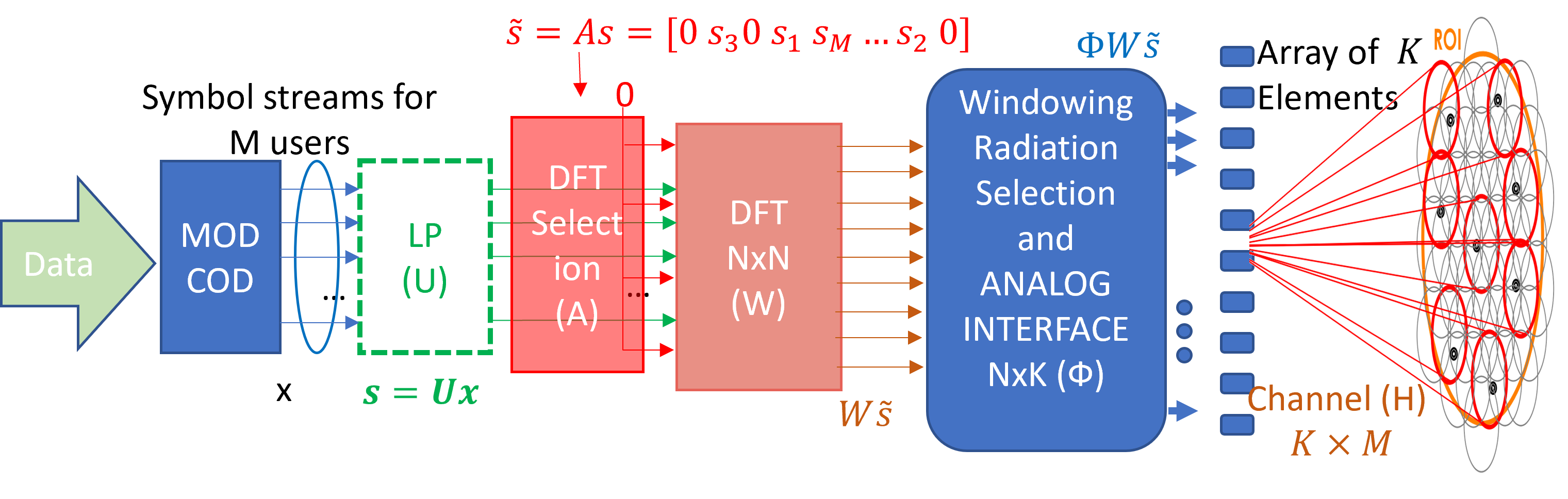
Figure 1: The broadband-signal architecture of the OBP-enabled MBS payload.

This paper aims to fill this gap by considering the joint design of both LP and DFT-based beamforming for the payloads of SATCOM systems. In particular, LP and DFT-vector (e.g., a column of the DFT matrix) selection are jointly designed for the forward-link (gateway$\rightsquigarrow$satellite$\rightsquigarrow$user equipment) to maximize the system achievable rate under a constraint on transmission power. To begin with, we formulate an optimization that takes into account all these design aspects. This problem considers the complex-valued variables corresponding to the LP design and the binary variables related to the DFT-vector selection mechanism, resulting in a mixed integer non-linear programming (MINP), which is NP-hard. The resulting problem is even more challenging due to the non-convex sum-rate objective function. To cope with this non-convex problem, we first transform it into an equivalent weighted minimum-mean-square-error (MMSE) problem. Then, an alternative approach is developed to solve the resulting weighted-MMSE problem, following which the LP and DFT-vector selection are iteratively updated. Notably, in each iteration, the LP is optimized by employing the duality method, while the DFT-vector selection task is re-formulated as a “job-employee” assignment problem which can be solved efficiently by the Hungarian method. In addition, a greedy algorithm is also proposed for comparison purposes. The computational complexity of these solutions is then analyzed. Finally, Monte Carlo simulations are performed to demonstrate the efficiency of the proposed designs.

The rest of this paper is organized as follows. In Section II we present the system model. Section III deals with the design and optimization of the joint precoding and beamforming schemes. Numerical results alongside their discussions appear in Section IV. Finally, concluding remarks are drawn in Section V.

Notations: Matrices and vectors are represented by uppercase and lowercase boldface letters, respectively. The transpose, conjugate, and Hermitian transpose operators are denoted as $(\cdot)^{T}$, $(\cdot)^{\prime}$, and $(\cdot)^{H}$, respectively.

II System Model and Problem Formulation

II-A System Model

Consider the forward-link of an OBP-enabled multi-beam satellite (MBS) system employing DFT-based beamforming technology to serve $M$ ground users, as illustrated in Fig. 1. In particular, the payload consists of six main components, namely: modulation and coding (MODCOD) block, linear precoding, DFT beam matching, DFT precoding, radiation selection, and analog interface.

II-A1 MODCOD Block

The “CODing” part refers to the overhead of forward error correction (FEC), whereas the “MODulation” implements the transformation from bit stream to an analog signal. Here, one assumes $M$ symbols are generated by the MODCOD block in one specific time slot due to the signal corresponding to $M$ users, denoted as $\mathbf{x}=[x_{1}\cdots x_{M}]$.

II-A2 Linear Precoding (LP)

It is a particular subclass of transmission schemes that enables serving multiple users sharing the same time-frequency resources simultaneously. Based on this, $M$ symbol streams are then coded independently and multiplied by an LP matrix $\mathbf{U}\in\mathbb{C}^{M\times M}$, which accounts for the precoding weights and power. The outputs of this block are $M$ baseband signals, namely $\mathbf{s}=\mathbf{U}\mathbf{x}$.

II-A3 DFT Beam Matching

This is a novel block introduced in this project for selecting the DFT-vector for each output of the LP block. Let $N>M$ be the size of the DFT-based beamforming vectors. If the $n$-th column, $\mathbf{w}_{n}$, of the DFT matrix is assigned to the symbol $s_{m}$ of $\mathbf{s}$, it means that the corresponding DFT beamforming vector applied to $s_{m}$ is $\mathbf{w}_{n}$. As the DFT matrix is $N\times N$, then “zeros” can be added if there is no symbol assigned to a specific input of the DFT vector. Our work aims to develop a matching framework to select the efficient DFT beamforming vectors for $\mathbf{s}$. To do so, we introduce the binary matrix $\mathbf{A}\in\mathbb{R}^{N\times M}$ whose $(n,m)$-th element, denoted by variable $a_{n,m}$, is defined as

$$a_{n,m}\!=\!\left\{\!\!\begin{array}[]{*{10}{l}}1,\!&\!\text{if the $n$-th DFT vector is assigned to $s_{m}$},\\ 0,\!&\!\text{otherwise}.\end{array}\right.$$ (1)

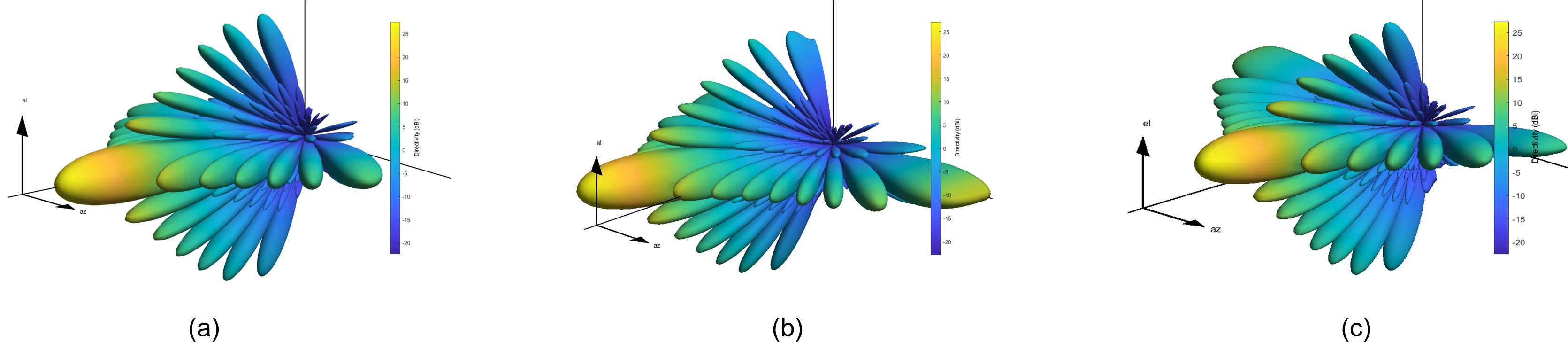
Figure 2: Examples of beam pattern corresponding to selected DFT-vector for $N=256$: (a) DFT-vector $\mathbf{w}_{1}$, (a) DFT-vector $\mathbf{w}_{5}$, and (c) DFT-vector $\mathbf{w}_{25}$.

Once DFT-vector $\mathbf{w}_{m}$ is assigned to $s_{m}$, the precoded signal $s_{m}$ can be propagated by the array element with a specific beam pattern. Some examples of propagation pattern for precoded signal are illustrated in Fig. 2. The constraints imposed on these binary variables are:

$$(C1):\sum_{\forall n}a_{n,m}=1,\forall m$$ (2)

$$(C2):\sum_{\forall m}a_{n,m}\leq 1,\forall n.$$ (3)

And the input of DFT block can be written as

$$\tilde{\mathbf{s}}=\mathbf{A}\mathbf{s}=\mathbf{A}\mathbf{U}\mathbf{x}.$$ (4)

II-A4 DFT beamforming

This block works on multiplying the baseband signals to the DFT beamforming matrix. Let $\mathbf{W}=[\mathbf{w}_{1}\,\mathbf{w}_{2}\,\cdots\,\mathbf{w}_{N}]\in\mathbb{C}^{N\times N}$ be the DFT matrix. Then, the outputs of DFT block can be described as

$$\mathbf{W}\tilde{\mathbf{s}}=\mathbf{W}\mathbf{A}\mathbf{s}=\mathbf{W}\mathbf{A}\mathbf{U}\mathbf{x}.$$ (5)

The computational complexity for directly implementing the $N$-point DFT via matrix multiplication is $N\times N$ complex multiplications and $N\times(N-1)$ complex additions, with an overall computational cost of $\mathcal{O}\left(N^{2}\right)$ [12]. Fast Fourier transform (FFT) techniques can be used to for lowering the computational cost of the DFT computation to $\mathcal{O}\left(N\log N\right)$, which explains why real-time beamformers can be better realized with less sophisticated circuitry and less power than matrix-by-vector multiplication. The FFT-based beamforming is an efficient way of improving the performance of the OBPs on satellite systems in terms of power reduction, mass, and throughput gain [12]. Furthermore, when compared to ideal payloads, an mMIMO payload architecture with fixed beamforming can achieve a considerable complexity reduction [10]. However, it is impossible to achieve the dynamic nature, i.e., steering the beam with respect to the motion of the satellite, with fixed beamforming alone. The precoding technique can be used to enable this dynamic capability.

II-A5 Spatial Windowing and Analog interface

In this stage, $K\leq N$ consecutive outputs from the DFT are selected (windowing), and each of them is connected to an antenna element through a radio-frequency (RF) chain (analog interface). The analog interface includes all the RF functionalities for transmission, such as up-converting baseband signals to RF signals and power amplification. Here, we assume that the matrix $\boldsymbol{\Phi}\in\mathbb{R}^{K\times N}$ is implemented before the analog interface, where each element of this matrix is zero or one (following a rectangular window distribution), and with $K$ denoting the number of radiation elements of the antenna array. Thus, the radiated signal can be written as $\boldsymbol{\Phi}\mathbf{W}\tilde{\mathbf{s}}$.

Downselecting the DFT outputs ($K<N$) increases the beamwidth of the formed beams, compared to its full utilization ($K=N$), due to the reduction of the array aperture. However, the system keeps the $N$ different beam-pointing directions as they depend on the incremental phase shifts generated by the DFT operation, which are maintained in the available $K$ antennas. Designing the array with a reduced number of elements may be required to comply with physical payload constraints, such as available area, mass, and power. On the other hand, the design can also be exploited to create overlapping beams, e.g., to avoid abrupt transitions in beam-hopping operations.

II-B Problem Formulation

Let $\mathbf{H}\in\mathbb{C}^{K\times M}$ be the channel matrix from the payload antenna array to the $M$ users. The signal received by the $M$ users can be written as

$$\mathbf{y}=\mathbf{H}^{H}\boldsymbol{\Phi}\mathbf{W}\mathbf{A}\mathbf{U}\mathbf{x}+\boldsymbol{\eta}=\tilde{\mathbf{H}}^{H}\mathbf{W}\mathbf{A}\mathbf{U}\mathbf{x}+\boldsymbol{\eta},$$ (6)

where $\tilde{\mathbf{H}}^{H}=\mathbf{H}^{H}\boldsymbol{\Phi}$. Thus, user $m$’s SINR of can be given as

$$\Gamma_{m}(\mathbf{U},\mathbf{A})=\dfrac{\|\tilde{\mathbf{h}}^{H}_{m}\mathbf{W}\mathbf{A}\mathbf{u}_{m}\|^{2}}{\sum_{j\neq m}\|\tilde{\mathbf{h}}^{H}_{m}\mathbf{W}\mathbf{A}\mathbf{u}_{j}\|^{2}+\sigma^{2}}\,,$$ (7)

where $\tilde{\mathbf{h}}_{m},\mathbf{u}_{m}$ are the $m$-th columns of matrices $\tilde{\mathbf{H}},\mathbf{U}$, respectively. Thus, the joint LP and DFT beamforming problem can be stated as

$$\underset{\mathbf{U},\mathbf{A}}{\max} \sum\limits_{\forall m}\log_{2}\left(1+\Gamma_{m}(\mathbf{U},\mathbf{A})\right)$$ (8b)

s.t. constraints $$(C1) (C2)$$, ,

$$(C3):\text{Trace}\left(\mathbf{U}^{H}\mathbf{U}\right)\leq P,$$

where $(C3)$ stands for the power constraint, and $P$ represents the transmission power budget. It is worth noting that problem (8) is non-convex MINP, which is well-known as NP-hard and thus non-trivial to solve. In particular, there is the coupling between the complex variables and binary ones. Additionally, the objective function is non-convex due to the presence of the mutual inter-user interference terms in the denominator of each user’s SINR.

III Optimization-based Solution Approach

III-A Weighted-MMSE-based Transformation

The non-convex problem (8) can be addressed by relating it to a weighted mean-sum square error (MSE) minimization problem as mentioned in the following theorem.

Theorem 1.

Problem (8) is equivalent to the following weighted MSE minimization problem, i.e. the two problems have same optimal points,

$$\underset{\mathbf{A},\mathbf{U},\left\{\delta_{m},\omega_{m}\right\}}{\min} g(\mathbf{U},\mathbf{A},\delta_{m},\omega_{m})=\sum\limits_{\forall m}\left(\omega_{m}e_{m}-\log\omega_{m}-1\right)$$ (9)

$$\mathrm{s.t.} (C1) (C2) (C3)$$ constraints , , and ,

where $e_{m}=\mathbb{E}\left[\big{|}x_{m}-\delta_{m}y_{m}\big{|}^{2}\right]$, $\omega_{m}$ and $\delta_{m}$ represent the MSE weight and the receiving coefficient for user $m$, respectively.

Proof:

The proof for this theorem is similar to that in [13, 14]. We omit the details for brevity. ∎

It is worth noting that the objective function in problem (9) is not jointly convex, but it is convex over each set of variables $\mathbf{u}_{m}$’s, $\mathbf{A}$, $\delta_{m}$’s, and $\omega_{m}$’s. Hence, an efficient algorithm for solving this problem can be developed by alternately optimizing $\mathbf{u}_{m}$’s and $\mathbf{A}$, and the MSE weight update for $\delta_{m}$’s, and $\omega_{m}$’s.

III-B Iterative LP-DFT Beamforming Design

III-B1 Update MSE Weights and Receive Coefficients

For given $(\mathbf{U},\mathbf{A})$, $\delta_{m}$’s, and $\omega_{m}$’s can be determined according to the results in [14]. In particular, the MMSE receiving coefficient at user $m$ is given as

$$\delta_{m}^{\star}=\delta_{m}^{\mathrm{MMSE}}=\bigg{(}\sum_{\forall j}|\tilde{\mathbf{h}}_{m}^{H}\mathbf{W}\mathbf{A}\mathbf{u}_{j}|^{2}+\sigma_{m}^{2}\bigg{)}^{-1}\mathbf{u}_{m}^{H}\mathbf{A}^{T}\mathbf{W}^{T}\tilde{\mathbf{h}}_{m}.$$ (10)

And, the optimum value of $\omega_{k}$ is expressed as

$$\omega_{m}^{\star}\!=\!e_{m}^{-1}\!=\!1\!+\!\bigg{(}\sum_{\forall j\neq m}|\tilde{\mathbf{h}}_{m}^{H}\mathbf{W}\mathbf{A}\mathbf{u}_{j}|^{2}+\sigma_{m}^{2}\bigg{)}^{-1}\!\!\!\!|\tilde{\mathbf{h}}_{m}^{H}\mathbf{W}\mathbf{A}\mathbf{u}_{m}|^{2}.$$ (11)

III-B2 Linear Precoding Design

For given $\delta_{m}$’s, $\omega_{m}$’s, and $\mathbf{A}$, one can define the LP by solving the following quadratically constrained quadratic program (QCQP):

$$\underset{\mathbf{U}}{\min}\sum\limits_{\forall m}\mathbf{u}_{m}^{H}\boldsymbol{\Theta}\mathbf{u}_{m}-2\omega_{m}\Re\left(\mathbf{k}_{m}^{H}\mathbf{u}_{m}\right)\;\mathrm{s.t.}\;\textrm{$(C3)$.}$$ (12)

where $\boldsymbol{\Theta}=\mathbf{A}^{T}\mathbf{W}^{T}\left(\sum_{\forall j}\omega_{j}|\delta_{j}|^{2}\tilde{\mathbf{h}}_{j}\tilde{\mathbf{h}}_{j}^{H}\right)\mathbf{W}\mathbf{A}$, $\mathbf{k}_{m}^{H}=\delta_{m}\tilde{\mathbf{h}}_{m}^{H}\mathbf{W}\mathbf{A}$, and $\Re(*)$ represents the real part. Since the above problem is a convex quadratic program, it can be solved by employing SDP transformation and CVX optimization tool as in [15] or utilizing the standard Lagrangian duality method. In particular, the Lagrangian of problem (12) is given by

$$\mathcal{L}(\mathbf{U},\beta)\!=\!\!\sum\limits_{\forall m}\!\left[\mathbf{u}_{m}^{H}(\boldsymbol{\Theta}+\beta\mathbf{I})\mathbf{u}_{m}\!-\!2\omega_{m}\Re\!\left(\mathbf{k}_{m}^{H}\mathbf{u}_{m}\right)\right]\!-\!\beta P,$$ (13)

where $\beta$ is the Lagrangian multiplier with respect to the constraints $(C3)$ and $\mathbf{I}$ stands for the $M\times M$ identity matrix. For given $\beta$, $\mathbf{u}_{m}$’s can be optimized in closed-form as

$$\mathbf{u}_{m}^{\star}=\arg\min_{\mathbf{u}_{m}}\mathcal{L}(\mathbf{U},\beta)=(\boldsymbol{\Theta}+\beta\mathbf{I})^{-1}\mathbf{k}_{m}\omega_{m}.$$ (14)

The dual function $\sf{g}(\beta)$ is then defined as $\sf{g}(\beta)=\inf_{\mathbf{U}}\mathcal{L}(\mathbf{U},\beta)$, and the dual problem can be stated as $\mathrm{max}_{\beta}\;\sf{g}(\beta)\;\mathrm{s.t.}\;\beta\geq 0$ which is convex by nature [16]. Hence, $\sf{g}(\beta)$ can be maximized by using the standard sub-gradient method where the dual variable $\beta$ can be iteratively updated as follows:

$$\beta^{[\ell+1]}=\left[\beta^{[\ell]}+r^{[\ell]}\left(\text{Trace}\left(\mathbf{U}^{H}\mathbf{U}\right)-P\right)\right]^{+},$$ (15)

where the suffix $[\ell]$ represents the iteration index, $r^{[\ell]}$ is the step size, and $[x]^{+}=\max(0,x)$. The convergence of this method can be guaranteed if $r^{[\ell]}$ is chosen appropriately so that $r^{[\ell]}\!\!\overset{\ell\rightarrow\infty}{\longrightarrow}\!\!0$ such as $r^{[\ell]}\!=\!1/\sqrt{\ell}$ [17, 16].

III-B3 DFT-vector Selection

Let $\mathbf{a}_{n}\in\mathbb{R}^{M\times 1}$ be the vector generated from the $n$-th row of $\mathbf{A}$. Substituting (6) into (9) and performing some minor manipulators, problem (9) can be rewritten as

$$\underset{\mathbf{A}}{\min}\sum\limits_{\forall n}\mathbf{a}_{n}^{T}\boldsymbol{\Psi}_{n}\mathbf{a}_{n}-2\left(\mathbf{f}_{n}^{T}\mathbf{a}_{n}\right)\;\mathrm{s.t.}\;\textrm{$(C1)$ and $(C2)$,}$$ (16)

where $\boldsymbol{\Psi}_{n}=\sum_{\forall m}\omega_{m}|\delta_{m}t_{m,n}^{\prime}|^{2}\sum_{\forall j}\mathbf{u}_{j}\mathbf{u}_{j}^{H}$, $t_{m,n}$ stands for the $n$-th element of vector $\mathbf{W}\tilde{\mathbf{h}}_{m}$, and $\mathbf{f}_{n}=\Re\left(\sum_{\forall m}\omega_{m}\delta_{m}t_{m,n}^{\prime}\mathbf{u}_{m}\right)$. It is a quadratic binary-optimization problem.

Theorem 2.

Problem (16) is equivalent to a “job-employee” assignment problem which can be solved by using the Hungarian method [18].

Proof:

Because $\mathbf{a}_{n}$ is a vector containing binary elements and its $\ell_{1}$-norm is less than $1$, i.e. $\|\mathbf{a}_{n}\|_{1}\leq 1$, according to $(C2)$, one can yield $\mathbf{a}_{n}^{T}\boldsymbol{\Psi}_{n}\mathbf{a}_{n}=\text{diag}(\boldsymbol{\Psi}_{n})^{T}\mathbf{a}_{n}$. Then, problem (16) can be rewritten as

$$\underset{\mathbf{A}}{\min}\sum\limits_{\forall(n,m)}\rho_{n,m}a_{n,m}\;\mathrm{s.t.}\;\textrm{$(C1)$ and $(C2)$,}$$ (17)

where $\rho_{n,m}$ is the $m$-th element of vector $(\text{diag}(\boldsymbol{\Psi}_{n})-2\mathbf{f}_{n})$. The formulation in (17) is a well-known “job-employee” assignment problem where $\rho_{n,m}$’s can be considered as the assignment weights [18]. ∎

III-B4 Algorithm Development

By iteratively updating $\delta_{m},\omega_{m},\mathbf{U}$, and $\mathbf{A}$ by solving problem (17), the LP matrix and DFT-vector selection can be obtained. The solution approach is summarized in Algorithm 1. Similar to the spirit presented in [13, 19], the alternating minimization process in Step 4–6 of our proposed algorithm results in a monotonic reduction of the objective function of (9); hence, the convergence of this algorithm can be guaranteed.

Algorithm 1 Iterative LP and DFT-selection Design

1:  Initialize:

1. Set $\mathbf{u}_{m}^{[0]}=\theta\mathbf{1}_{N\times 1}$ for all $m$, where $\theta$ is sufficiently small to not violate constraint $(C3)$.

2. Randomly select $\{a_{n,m}\}$’s satisfying constraint $(C1)$ and $(C2)$.

3. Set $\ell=0$ and select initial value $\beta^{[0]}\geq 0$.

2:  repeat

3:     Update $\ell:=\ell+1$ and $\beta^{[\ell]}$ as in (15).

4:     Define $\left\{\delta_{m}^{[\ell]}\right\}$’s and $\left\{\omega_{m}^{[\ell]}\right\}$’s as in (10) and (11), respectively.

5:     Calculate $\mathbf{U}^{[\ell]}$ as described in (14).

6:     Update $\mathbf{A}^{[l]}$ by employing Hungarian method to solve (17).

7:  until Convergence.

III-C Greedy Algorithm

To lessen the complexity level in solving problem (8), we introduce a greedy algorithm in this section. Following this approach, the binary matrix $\mathbf{A}$ can be determined by step-by-step picking the DFT vector having strong impact on each user. Once $\mathbf{A}$ is defined, we can employ the zero-forcing (ZF) design to compute $\mathbf{U}$. In particular, this greedy solution method is summarized in Algorithm 2.

Algorithm 2 Greedy Algorithm

1:  Initialization: Set $\mathcal{N}=\{1,2,...,N\}$.

2:  for $m=1$ to $M$ do

3:     We define the index of the best DFT vector for user $m$ as $n_{m}^{\star}=\underset{n\in\mathcal{N}}{\operatorname*{arg\;max}}|\tilde{\mathbf{h}}_{m}^{H}\mathbf{w}_{n}|^{2}$.

4:     Set $a_{n_{m}^{\star},m}=1$, and $a_{n,m}=0$ for all $n\neq n_{m}^{\star}$.

5:     Update $\mathcal{N}=\mathcal{N}\setminus\{n_{m}^{\star}\}$.

6:  end for

7:  Define $\mathbf{U}_{\sf{ZF}}=\mathbf{Q}^{H}\left(\mathbf{Q}\mathbf{Q}^{H}\right)^{-1}$ where $\mathbf{Q}^{H}=\mathbf{H}^{H}\boldsymbol{\Phi}\mathbf{W}\mathbf{A}$.

III-D Complexity Analysis

In this section, we investigate the complexities of our two proposed approaches. To begin with, it is observed that the major complexity of each iteration of implementing Algorithm 1 is to solve the problem 17by using the Hungarian method. As reported in [18], the complexity of the Hungarian algorithm is $\mathcal{O}(N^{3})$. In addition, according to [20], the number of iterations of the gradient descent method employed in Algorithm 1 can be of $\mathcal{O}\left(\xi_{\sf{Alg.1}}^{-1}\right)$ where $\xi_{\sf{Alg.1}}$ represents the solution accuracy for solving problem (8). The complexity of this algorithm can be estimated as

$$X_{\sf{Alg.1}}=\mathcal{O}(\xi_{\sf{Alg.1}}^{-1}\times N^{3}).$$ (18)

Next, Algorithm 2 involves a for-loop to select the best corresponding DFT vector for each user in Steps 2-6 and the ZF approach to computing $\mathbf{U}$. Hence, the complexity of the greedy algorithm is of

$$X_{\sf{Alg.2}}=\mathcal{O}(N^{2}+M^{3}).$$ (19)

The complexity analysis results seem highly suitable for practical implementations since its power consumption is not increased, taking into account that the update rate of the algorithm can be very low and dictated by the variations over time of the channel response.

IV Simulation Results

TABLE I: Simulation Parameters

Number of Monte Carlo simulations	$50$
Forward link carrier frequency	$19$ GHz
Link bandwidth,	$500$ MHz
MEO attitude	$8000$ km
Earth radius	$6378$ km
Total payload RF power	$1.0-3.0$ kW
Minimum satellite elevation angle	$5$ degrees
Number of simulated users	$20-50$
Uniform rectangular array (URA) size	$8\times 8-12\times 12$
Array element normalized spacing ($d_{A}/\lambda$)	$0.5-1.5$
Array element radiation model	Cosine
FFT size	256
User terminal antenna gain	$41.45$ dBi
Temperature at user terminals	$224.5$ K
Channel Model	Refer to [10]

In this section, Monte Carlo simulations are conducted to assess the performance of the proposed algorithms. A MEO satellite communication scheme with a payload equipped with a uniform rectangular array (URA) antenna is considered. Table I summarizes the key system parameters adopted for the following numerical simulations. For benchmarking, the simulation results also include fully digital precoding (FDP) designs using match-filter (MF) and MMSE approaches presented in [10], as well as DFT beamforming (Algorithm 2 without LP design). In Figs. 3-6, we show the total achievable rate obtained by different schemes versus the total transmission power $P$, the number of users, the URA size, and the normalized array element spacing, respectively. Unless the setting parameters are stated in a specific range of values for simulation, we set $P=3000~{}W$, $M=45$, URA size of $10\times 10$, and $d_{A}/\lambda=1$.

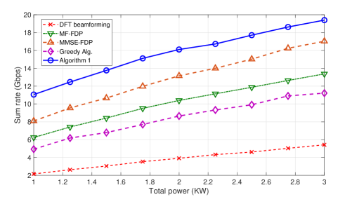
Figure 3: The achievable sum rate versus the transmission power.

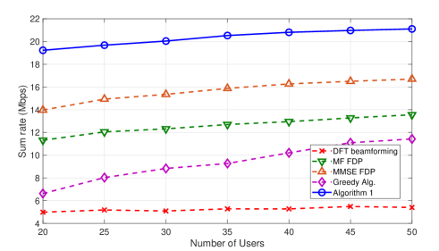
Figure 4: The achievable sum rate versus the number of users.

As can be seen, Algorithm 2 is significantly superior to “DFT beamforming” scheme in all simulations. This has shown that employing the LP design on top of DFT beamforming can improve the network performance in terms of achievable rate, as expected. Furthermore, Figs. 3-6 indicate that Algorithm 1 always outperforms Algorithm 2. Learning from these results, one can clearly confirm the advantages of using the jointly designed LP and DFT beamforming. Interestingly, our joint LP-DFT design can return a higher achievable rate than both traditional precoding approaches match-filter (“MF-FDP”) and MMSE (““MMSE-FDP””) significantly.

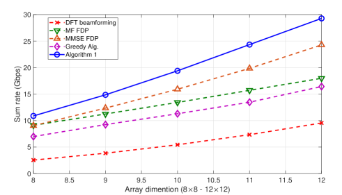
Figure 5: The achievable sum rate versus the number of antennas.

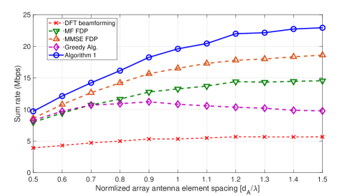
Figure 6: The achievable sum rate versus the normalized array element spacing.

As observed from Fig. 3, the achievable rates from all algorithms increase as the transmission power increases. It is impressing that the employing LP technique on top of DFT beamforming, i.e., Algorithm 2, can roundly double the achievable rate in comparison to the scheme exploiting only the later technique. In addition, jointly designing these two can further gain more than $3$ or $4$ Gbps when $P$ varies from $1$ to $3$ kW. In Figs. 4 and 5, we study that a larger number of users or antennas results in higher total achievable rate for all schemes in Fig. 4. Similarly, as shown in Fig. 6, setting a larger separation between array elements can enhance the system capacity of all schemes but the greedy algorithm.

V Conclusion

In this paper, we have developed the joint LP and DFT-beamforming designs for OBP-enabled payloads in satellite communication systems. In particular, an efficient algorithm that iteratively and jointly optimizes the linear precoding and DFT-beamforming selection has been proposed to maximize the network throughput under transmission power constraints. Monte Carlo simulation results with various network parameter settings have illustrated the effectiveness of our proposed algorithms in improving the network capacity.

References

- [1] M. Centenaro, C. E. Costa, F. Granelli, C. Sacchi, and L. Vangelista, “A survey on technologies, standards and open challenges in satellite iot,” IEEE Communications Surveys & Tutorials, vol. 23, no. 3, pp. 1693–1720, 2021.
- [2] J. Ye, J. Qiao, A. Kammoun, and M.-S. Alouini, “Non-terrestrial communications assisted by reconfigurable intelligent surfaces,” Proceedings of the IEEE, 2022.
- [3] V. N. Ha, T. T. Nguyen, E. Lagunas, J. C. M. Duncan, and S. Chatzinotas, “Geo payload power minimization: Joint precoding and beam hopping design,” 2022. [Online]. Available: https://arxiv.org/abs/2208.10474
- [4] L. Chen, V. N. Ha, E. Lagunas, L. Wu, S. Chatzinotas, and B. Ottersten, “The next generation of beam hopping satellite systems: Dynamic beam illumination with selective precoding,” IEEE Transactions on Wireless Communications, 2022.
- [5] E. Lagunas, V. N. Ha, V. C. Trinh, S. Andrenacci, N. Mazzali, and S. Chatzinotas, “Multicast mmse-based precoded satellite systems: User scheduling and equivalent channel impact,” in VTC-Fall 2022, 2022, pp. 1–6.
- [6] L. You, K.-X. Li, J. Wang, X. Gao, X.-G. Xia, and B. Ottersten, “Massive mimo transmission for leo satellite communications,” IEEE Journal on Selected Areas in Communications, vol. 38, no. 8, pp. 1851–1865, 2020.
- [7] Y. Liu, C. Li, J. Li, and L. Feng, “Robust Energy-Efficient Hybrid Beamforming Design for Massive MIMO LEO Satellite Communication Systems,” IEEE Access, vol. 10, pp. 63 085–63 099, 2022.
- [8] Y. Zhang, A. Liu, P. Li, and S. Jiang, “Deep Learning (DL)-Based Channel Prediction and Hybrid Beamforming for LEO Satellite Massive MIMO System,” IEEE Internet of Things Journal, pp. 1–1, 2022.
- [9] F. Vidal, H. Legay, G. Goussetis, and J.-P. Fraysse, “Joint precoding and resource allocation strategies applied to a large direct radiating array for geo telecom satellite applications,” in 2021 15th European Conference on Antennas and Propagation (EuCAP), 2021, pp. 1–5.
- [10] P. Angeletti and R. De Gaudenzi, “A Pragmatic Approach to Massive MIMO for Broadband Communication Satellites,” IEEE Access, vol. 8, pp. 132 212–132 236, 2020.
- [11] ESA Project EGERTON, “Efficient digital beamforming techniques for onboard digital processors,” https://wwwen.uni.lu/snt/research/sigcom/projects/egerton, 2021, [Online; accessed 15-July-2022].
- [12] R. Palisetty, G. Eappen, J. L. G. Rios, J. C. M. Duncan, S. Domouchtsidis, S. Chatzinotas, B. Ottersten, B. Cortazar, S. D’Addio, and P. Angeletti, “Area-power analysis of fft based digital beamforming for geo, meo, and leo scenarios,” in 2022 IEEE 95th Vehicular Technology Conference: (VTC2022-Spring), 2022, pp. 1–5.
- [13] S. S. Christensen, R. Agarwal, E. de Carvalho, and J. M. Cioffi, “Weighted sum-rate maximization using weighted mmse for mimo-bc beamforming design,” in 2009 IEEE International Conference on Communications, 2009, pp. 1–6.
- [14] V. N. Ha, D. H. N. Nguyen, and J.-F. Frigon, “Subchannel allocation and hybrid precoding in millimeter-wave ofdma systems,” IEEE Transactions on Wireless Communications, vol. 17, no. 9, pp. 5900–5914, 2018.
- [15] V. N. Ha, L. B. Le, and N.-D. Đào, “Coordinated multipoint transmission design for cloud-rans with limited fronthaul capacity constraints,” IEEE Transactions on Vehicular Technology, vol. 65, no. 9, pp. 7432–7447, 2016.
- [16] S. Boyd and L. Vandenberghe, Convex Optimization. Cambridge University Press, March 2004. [Online]. Available: http://www.amazon.com/exec/obidos/redirect?tag=citeulike-20&path=ASIN/0521833787
- [17] V. N. Ha and L. B. Le, “End-to-end network slicing in virtualized ofdma-based cloud radio access networks,” IEEE Access, vol. 5, pp. 18 675–18 691, 2017.
- [18] D. Jungnickel, Weighted Matchings. Berlin, Heidelberg: Springer Berlin Heidelberg, 2013, pp. 441–479. [Online]. Available: https://doi.org/10.1007/978-3-642-32278-5_14
- [19] V. N. Ha, D. H. N. Nguyen, and J.-F. Frigon, “System energy-efficient hybrid beamforming for mmwave multi-user systems,” IEEE Transactions on Green Communications and Networking, vol. 4, no. 4, pp. 1010–1023, 2020.
- [20] K. Yuan, Q. Ling, and W. Yin, “On the convergence of decentralized gradient descent,” SIAM Journal on Optimization, vol. 26, no. 3, pp. 1835–1854, 2016. [Online]. Available: https://doi.org/10.1137/130943170