Integrable systems on the sphere, ellipsoid and hyperboloid

Abstract

Affine transformations in Euclidean space generates a correspondence between integrable systems on cotangent bundles to the sphere, ellipsoid and hyperboloid embedded in $R^{n}$. Using this correspondence and the suitable coupling constant transformations we can get real integrals of motion in the hyperboloid case starting with real integrals of motion in the sphere case. We discuss a few such integrable systems with invariants which are cubic, quartic and sextic polynomials in momenta.

1 Introduction

According to [43] integrable systems on the hyperboloid were not studied in detail, partly because the generalisation from the ellipsoid case seems to be obvious. The main difference is the existence of non-compact trajectories coming from infinity and going away to infinity, which allows us to study scattering on hyperboloids.

On the sphere there are integrable systems with polynomial invariants of second, third, fourth and sixth order in momenta [3, 4, 19, 35, 38, 40]. We want to discuss the counterparts of these polynomial invariants on the ellipsoid and hyperboloid. After the construction of integrals of motion, we will be able to proceed to the study of the properties of noncompact trajectories on hyperboloid [43].

In the 19 century, Cayley and Klein discovered that Euclidean and non-Euclidean geometries can be considered as mathematical structures living inside projective metric spaces [6, 29, 31, 46, 47]. The concept of a Cayley-Klein geometry leads to a unified description and classification of a wide range of the integrable systems. Nevertheless, the modern literature still divides integrable systems on the sphere, ellipsoid or hyperboloid, see [2, 4, 7, 16, 17, 18, 20, 21, 24, 25, 38, 39, 42, 43, 48] and references within.

The Cayley-Klein algebra can be defined as a graded contracted Lie algebra $so(n)$ depending on $n-1$ contraction parameters. For instance, the Poisson bracket on $so^{*}(3)$

$$\{J_{1},J_{2}\}=J_{3}\,,\quad\{J_{2},J_{3}\}=J_{1}\,,\quad\{J_{3},J_{1}\}=J_{2}$$ (1.1)

are replaced on the Poisson bracket depending on parameters $\kappa_{1}$ and $\kappa_{2}$

$$\{J_{1},J_{2}\}_{\kappa}=J_{3}\,,\quad\{J_{2},J_{3}\}_{\kappa}=\kappa_{1}J_{1}\,,\quad\{J_{3},J_{1}\}_{\kappa}=\kappa_{2}J_{2}\,,$$

see discussion of the corresponding geometries and integrable systems in [14].

The main disadvantage of such deformation is the following, if we know integrals of motion, Lax matrices, $r$-matrices, variables of separation and Abel’s quadratures on $so^{*}(n)$ we have to re-do a series of technical calculations to construct integrals of motion, Lax matrices, $r$-matrices, variables of separation and Abel’s quadratures depending on contraction parameters $\kappa_{i}$, see examples in [4, 13, 14, 22, 23, 5, 28].

In this note, we study different symplectic realizations of the Lie-Poisson bracket without its deformation, following Novikov and Schmelzer paper [27]. For instance, there is a well-known realization of $so^{*}(3)$ variables

$$J_{1}=p_{3}x_{2}-p_{2}x_{3}\,,\qquad J_{2}=p_{1}x_{3}-p_{3}x_{1}\,,\qquad J_{3}=p_{2}x_{1}-p_{1}x_{2}\,,$$ (1.2)

associated with the angular momentum map [27]. Another symplectic realization

$$J_{1}=\dfrac{a_{3}p_{3}x_{2}-a_{2}p_{2}x_{3}}{\sqrt{a_{2}}\sqrt{a_{3}}}\,,\quad J_{2}=\dfrac{a_{1}p_{1}x_{3}-a_{3}p_{3}x_{1}}{\sqrt{a_{1}}\sqrt{a_{3}}}\,,\quad J_{3}=\dfrac{a_{2}p_{2}x_{1}-a_{1}p_{1}x_{2}}{\sqrt{a_{1}}\sqrt{a_{2}}}\,,$$ (1.3)

can be obtained from (1.2) by using affine transformations in Euclidean space $R^{3}$. Here $a_{i}$ are squares of the semi-axes of the ellipsoid/hyperboloid and

• if $x_{i}$ and $p_{i}$ satisfy the Dirac-Poisson bracket on cotangent bundle to the sphere $T^{*}S^{3}$, variables $J_{i}$ (1.2) satisfy to the Lie-Poisson bracket (1.1);

• if $x_{i}$ and $p_{i}$ satisfy the Dirac-Poisson bracket on the cotangent bundle to the ellipsoid $T^{*}E^{3}$, or hyperboloid $T^{*}H^{3}$, then variables $J_{i}$ (1.3) satisfy to the same Lie-Poisson bracket (1.1).

It allows us to express integrals of motion, Lax matrices, $r$-matrices, variables of separation and Abel’s quadratures in variables $(x,J)$-variables and then study these objects depending on parameters $a_{i}$ on the sphere, ellipsoid and hyperboloid.

If some parameters $a_{i}<0$ then realisation (1.3) is defined over a complex number field. Our main aim is to show that additional transformation of the coupling constants in Hamiltonians allows us to real Hamiltonians for the ellipsoid and hyperboloid cases starting with well-known real Hamiltonians for the sphere case. In physics, a coupling constant or interaction constant is a number that determines the strength of the force exerted in an interaction.

2 Dirac brackets on the sphere, ellipsoid and hyperboloid

Let us consider unit sphere $S^{n-1}$, ellipsoid $E^{n-1}$ and hyperboloid $H^{n-1}$ embedded in Euclidean space $R^{n}$.

Cotangent bundles to the sphere, ellipsoid and hyperboloid are defined by two second-class constraints in $T^{*}R^{n}$

$$F_{1}=\frac{x_{1}^{2}}{a_{1}}+\frac{x_{2}^{2}}{a_{2}}+\cdots+\frac{x_{n}^{2}}{a_{n}}-1=0,\quad\mbox{and}\quad F_{2}=\frac{x_{1}p_{1}}{a_{1}}+\frac{x_{2}p_{2}}{a_{2}}+\cdots+\frac{x_{n}p_{n}}{a_{n}}=0\,.$$

Here $x_{i}$ are Cartesian coordinates in configuration Euclidean space $R^{n}$, $p_{i}$ are momenta in phase space $T^{*}R^{n}$ and parameters $a_{1},\cdots,a_{n}$ are real numbers so that

• for the unit sphere $S^{n-1}$

  $$a_{1}=a_{2}=\cdots=a_{n}=1,$$

• for the ellipsoid $E^{n-1}$

  $$0<a_{1}<a_{2}<\cdots<a_{n},$$

• for the one-sheet hyperboloid $H^{n-1}$

  $$a_{1}<0<a_{2}<\cdots<a_{n},$$

and so on.

Canonical Poisson bracket on the cotangent bundle $T^{*}R^{n}$

$$\{x_{i},x_{j}\}=\{p_{i},p_{j}\}=0\,,\qquad\{x_{i},p_{j}\}=\delta_{ij}\,,\qquad i,j=1,\ldots,n$$ (2.4)

defines Dirac-Poisson bracket which is restrictions of (2.4) to the constraint surfaces

$$\{f,g\}_{D}=\{f,g\}-\dfrac{\{F_{1},f\}\{F_{2},g\}-\{F_{1},g\}\{F_{2},f\}}{\{F_{1},F_{2}\}}\,,$$ (2.5)

see [8].

When $a_{i}=1$ the Dirac-Poisson bracket in the sphere case has the following form

$$\{x_{i},x_{j}\}_{S}=0\,,\quad\{p_{i},x_{j}\}_{S}=\delta_{ij}-x_{i}x_{j}\,,\quad\{p_{i},p_{j}\}_{S}=x_{j}p_{i}-x_{i}p_{j}.$$ (2.6)

For the ellipsoid and hyperboloid cases, the Dirac-Poisson brackets of the coordinate functions are

$$\{x_{i},x_{j}\}_{D}=0\,,\quad\{p_{i},x_{j}\}_{D}=\delta_{ij}-\frac{x_{i}x_{j}}{a_{i}a_{j}(A^{-2}x,x)}\,,\quad\{p_{i},p_{j}\}_{D}=-\frac{x_{i}p_{j}-x_{j}p_{i}}{a_{i}a_{j}(A^{-2}x,x)}\,,$$ (2.7)

where $A=diag(a_{1},a_{2},a_{3})$ is the diagonal matrix. We have Dirac-Poison bracket (2.7) over a real numbers field both for positive and negative real parameters $a_{i}$ .

2.1 Affine transformation relating sphere and ellipsoid

Ellipsoid is an affine image of the unit sphere, i.e. affine transformation in Euclidean space

$$x_{i}\to\frac{x_{i}}{\sqrt{a_{i}}}$$

changes first constraint in an appropriate way

$$F_{1}=\sum_{i=1}^{n}x_{i}^{2}-1=0\qquad\to\qquad F_{1}=\sum_{i=1}^{n}\frac{x_{i}^{2}}{a_{i}}-1=0\,.$$

By adding suitable transformation of momenta $p_{i}\to{p_{i}}/{\sqrt{a_{i}}}$ we also change the second constraint in the way we need

$$F_{2}=\sum_{i=1}^{n}x_{i}p_{i}=0\qquad\to\qquad F_{2}=\sum_{i=1}^{n}\frac{x_{i}p_{i}}{a_{i}}=0\,.$$

Thus, the transformation of variables

$$x_{i}\to\frac{x_{i}}{\sqrt{a_{i}}}\qquad\mbox{and}\qquad p_{i}\to\frac{p_{i}}{\sqrt{a_{i}}}$$

maps manifold $T^{*}S^{n-1}$ to $T^{*}E^{n-1}$ or $T^{*}H^{n-1}$, but changes both symplectic 2-form $\omega=q\wedge p$ in $T^{*}R^{n}$ and the corresponding Dirac bracket.

Canonical transformation

$$x_{i}\to\frac{x_{i}}{\sqrt{a_{i}}}\qquad\mbox{and}\qquad p_{i}\to\sqrt{a_{i}}p_{i}$$ (2.8)

preserves $\omega=q\wedge p$ and, simultaneously, the second constraint

$$F_{2}=\sum_{i=1}^{n}x_{i}p_{i}=0\qquad\to\qquad F_{2}=\sum_{i=1}^{n}x_{i}p_{i}=0\,.$$

Thus, canonical transformation (2.8) does not map $T^{*}S^{n-1}$ to $T^{*}E^{n-1}$ or $T^{*}H^{n-1}$.

2.2 Momentum map

According to [27] symplectic manifold $T^{*}S^{2}$ is symplectomorphic to a partial symplectic leaf of the Euclidean algebra $e^{*}(3)$. Therefore, we proceed from symplectic manifold $T^{*}R^{n}$ and its hypersurfaces to the Poisson manifold $e^{*}(n)$ because preserving Poisson bracket transformations also preserve symplectic leaves.

Following [27] we consider the angular momentum map which defines a Poisson morphism

$$\mu:\qquad T^{*}S^{n-1}\to e^{*}(n)$$ (2.9)

between symplectic manifold $T^{*}S^{n-1}$ equipped with Dirac-Poisson bracket (2.5) and symplectic leaf of the Euclidean algebra $e^{*}(n)=so^{*}(n)\ltimes R^{n}$ equipped with the standard Lie-Poisson bracket

$$\begin{array}[]{l}\{J_{ij},J_{km}\}=\delta_{im}J_{kj}-\delta_{jk}J_{im}+\delta_{ik}J_{jm}-\delta_{jm}J_{ki}\,,\\ \\ \{J_{ij},x_{k}\}=\delta_{ik}x_{j}-\delta_{jk}x_{i}\,,\qquad\{x_{i},x_{j}\}=0\,.\end{array}$$ (2.10)

The angular momentum map $\mu$ relates two vectors $x$ and $p$ with vector $x$ and angular momentum operator $\mathbf{J}\in so^{*}(n)$

$$\mu:\qquad(x,p)\to(x,\mathbf{J})\,,$$

where $\mathbf{J}$ is a skew-symmetric matrix with entries

$$J_{ij}=x_{i}p_{j}-x_{j}p_{i}\,.$$

Canonical transformation (2.8) preserves both canonical Poisson bracket (2.4) on $T^{*}R^{n}$ and the Lie-Poisson bracket on $e^{*}(n)$ (2.10) together with necessary to our purpose symplectic leaves.

Thus, we have variables $(y,\mathbf{L})$

$$y_{i}=\frac{x_{i}}{\sqrt{a_{i}}}\qquad\mbox{and}\qquad L_{ij}=\frac{a_{j}x_{i}p_{j}-a_{i}x_{j}p_{i}}{\sqrt{a_{i}}\sqrt{a_{j}}}\,,$$

which satisfy to the same Lie-Poisson bracket as variables $(x,\mathbf{J})$ (2.10). The momentum map depending on parameters $a_{i}$

$$\mu_{a}:\qquad(x,p)\to(y,\mathbf{L})\,,$$

is a Poisson morphism between cotangent bundles $T^{*}E^{n-1}$ or $T^{*}H^{n-1}$ equipped with Dirac-Poisson bracket and the symplectic leaf of the Euclidean algebra $e^{*}(n)$ over fields of real and complex numbers, respectively.

Thus, if we know a set of independent integrals of motion in the involution on the cotangent bundle to the sphere

$$\{H_{i},H_{j}\}_{S}=0\,,\qquad i,j=1,\ldots n-1\,,$$ (2.11)

we can

• rewrite integrals of motion in terms of the real variables $(x,\mathbf{J})$ on $e^{*}(n)$;

• substitute reals variables $(y,\mathbf{L})$ instead of variables $(x,\mathbf{J})$;

• rewrite integrals of motion in terms of the variables $(x,p)$ for the ellipsoid;

• change sign $a_{i}\to-a_{i}$ of some parameters and calculate integrals of motion $H_{i}$ depending on real variables $(x,p)$ and complex numbers $\sqrt{a_{i}}$, which are independent and commute for each other with respect to Dirac-Poisson bracket in the hyperboloid case;

• try to construct real integrals of motion $H_{i}$ replacing real coupling constant to the complex one.

In the hyperboloid case intermediate variables $(y,\mathbf{L})$ are defined over a field of hypercomplex numbers in full accordance with the general theory [6, 46, 47].

Additional transformation of the coupling constant usually allows us to change complex numbers $\sqrt{a_{i}}$ to real ones and to obtain real integrals of motion on the hyperboloid starting with known real integrals of motion on the sphere. Below we present examples for several classical integrable systems on the sphere.

2.3 Three-dimensional Euclidean space

Six-dimensional Euclidean algebra $e(3)=so(3)\ltimes R^{3}$ is a semidirect product of the Lie algebra of skew-symmetric $3\times 3$ matrices with real entries and the abelian Lie algebra of three-dimensional vectors with coordinates

$$\mathbf{J}=\left(\begin{array}[]{ccc}0&J_{3}&-J_{2}\\ -J_{3}&0&J_{1}\\ J_{2}&-J_{1}&0\\ \end{array}\right)\qquad\mbox{and}\qquad x=\left(\begin{array}[]{c}x_{1}\\ x_{2}\\ x_{3}\\ \end{array}\right)\,.$$

The Lie-Poisson structure on its dual as a vector space algebra $e^{*}(3)$ reads as

$$\{J_{i}\,,J_{j}\}=\varepsilon_{ijk}J_{k}\,,\qquad\{x_{i}\,,J_{j}\}=\varepsilon_{ijk}x_{k}\,,\qquad\{x_{i}\,,x_{j}\}=0\,,$$ (2.12)

where $\varepsilon_{ijk}$ is a skew-symmetric tensor so that

$$\{J_{1},J_{2}\}=J_{3}\,,\qquad\{J_{2},J_{3}\}=J_{1}\,,\qquad\{J_{3},J_{1}\}=J_{2}\,.$$

This Poisson bracket has two Casimir functions

$$C_{1}=x_{1}^{2}+x_{2}^{2}+x_{3}^{2}\qquad\mbox{and}\qquad C_{2}=x_{1}J_{1}+x_{2}J_{2}+x_{3}J_{3}.$$

Fixing their values

$$C_{1}=1\qquad\mbox{and}\qquad C_{2}=0\,,$$ (2.13)

we obtain a symplectic leaf which is symplectomorphic to the cotangent bundle of the unit sphere, All detail may be found in the Novikov and Schmelzer paper [27].

2.3.1 Two dimensional sphere

At $n=3$ the Poisson bracket between coordinates $x=(x_{1},x_{2},x_{3})$ and momenta $p=(p_{1},p_{2},p_{3})$ are

$$\{x_{i},x_{j}\}=\{p_{i},p_{j}\}=0\,,\qquad\{x_{i},p_{j}\}=\delta_{ij}\,,\qquad i,j=1,\ldots,3.$$ (2.14)

The unit two dimensional sphere $S^{2}$ and its cotangent bundle $T^{*}S^{2}$ are defined via constraints

$$F_{1}=x_{1}^{2}+x_{2}^{2}+x_{3}^{2}=1\,,\quad\mbox{and}\quad F_{2}=x_{1}p_{1}+x_{2}p_{2}+x_{3}p_{3}=0\,.$$

Induced symplectic structure on $T^{*}S^{2}$ is given by the Dirac-Poisson bracket (2.6).

Proposition 1

The Dirac-Poisson bracket (2.6) between entries

$$J_{1}=p_{3}x_{2}-p_{2}x_{3}\,,\qquad J_{2}=p_{1}x_{3}-p_{3}x_{1}\,,\qquad J_{3}=p_{2}x_{1}-p_{1}x_{2}\,,$$ (2.15)

of the angular momentum vector $J=x\times p$ and coordinates $x$ have the form

$$\{J_{i}\,,J_{j}\}_{S}=\varepsilon_{ijk}J_{k}\,,\qquad\{x_{i}\,,J_{j}\}_{S}=\varepsilon_{ijk}x_{k}\,,\qquad\{x_{i}\,,x_{j}\}_{S}=0\,.$$

It allows us to consider this Dirac-Poisson bracket $\{.,.\}_{S}$ as a symplectic realization of the Lie-Poisson bracket (2.12) on the partial symplectic leaf defined by

$$C_{1}=x_{1}^{2}+x_{2}^{2}+x_{3}^{2}=1\quad\mbox{and}\quad C_{2}=x_{1}J_{1}+x_{2}J_{2}+x_{3}J_{3}=0.$$

The proof is a straightforward verification of the Poisson brackets between $(x,J)$-variables and values of the Casimir functions.

2.3.2 Two-dimensional ellipsoid and hyperboloid

The cotangent bundle to the ellipsoid or hyperboloid is defined by the following two constraints

$$F_{1}=\frac{x_{1}^{2}}{a_{1}}+\frac{x_{1}^{2}}{a_{2}}+\frac{x_{1}^{2}}{a_{2}}-1=0,\qquad F_{2}=\frac{x_{1}p_{1}}{a_{1}}+\frac{x_{2}p_{2}}{a_{2}}+\frac{x_{3}p_{3}}{a_{3}}=0\,.$$ (2.16)

The corresponding Dirac-Poisson bracket (2.5) is given by (2.7).

Proposition 2

The Dirac-Poisson bracket (2.7) between variables

$$y_{1}=\dfrac{x_{1}}{\sqrt{a_{1}}}\,,\qquad y_{2}=\dfrac{x_{2}}{\sqrt{a_{2}}}\,,\qquad y_{3}=\dfrac{x_{3}}{\sqrt{a_{3}}}\,.$$ (2.17)

and

$$L_{1}=\dfrac{a_{3}p_{3}x_{2}-a_{2}p_{2}x_{3}}{\sqrt{a_{2}}\sqrt{a_{3}}}\,,\quad L_{2}=\dfrac{a_{1}p_{1}x_{3}-a_{3}p_{3}x_{1}}{\sqrt{a_{1}}\sqrt{a_{3}}}\,,\quad L_{3}=\dfrac{a_{2}p_{2}x_{1}-a_{1}p_{1}x_{2}}{\sqrt{a_{1}}\sqrt{a_{2}}}\,.$$ (2.18)

are equal to

$$\{L_{i}\,,L_{j}\}_{D}=\varepsilon_{ijk}L_{k}\,,\qquad\{y_{i}\,,L_{j}\}_{D}=\varepsilon_{ijk}y_{k}\,,\qquad\{y_{i}\,,y_{j}\}_{D}=0\,.$$

It allows us to consider this Dirac-Poisson bracket $\{.,.\}_{D}$ as symplectic realization of the Lie-Poisson bracket (2.12) on the partial symplectic leaf defined by

$$C_{1}=y_{1}^{2}+y_{2}^{2}+y_{3}^{2}=1\quad\mbox{and}\quad C_{2}=y_{1}L_{1}+y_{2}L_{2}+y_{3}L_{3}=0.$$

The proof is a straightforward verification of the Poisson brackets between $(y,L)$-variables and values of the Casimir functions.

3 Examples of real integrals of motion in the hyperboloid case

For the sphere, ellipsoid case and hyperboloid case we have a common Lie-Poisson bracket (2.12) over fields of real and complex numbers (hypercomplex), respectively [6, 46, 47]. Since the choice of the field does not affect the involution of integrals of motion

$$\{H_{i},H_{j}\}=0\,,$$

on the existence of the Lax matrices, variables of separation and Abel’s quadratures, we can use canonical transformation (2.8) to construct integrable systems on a hyperbolic space.

In this section, we study the transformation of the coupling constants which allows us to get real Hamiltonians in this way.

3.1 Neumann system

Following [3, 20, 21] we start with the Neumann system on the sphere $S^{2}$ defined by Hamiltonian

$$H=a_{1}J_{1}^{2}+a_{2}J_{2}^{2}+a_{3}J_{3}+a_{2}a_{3}x_{1}^{2}+a_{1}a_{3}x_{2}^{2}+a_{1}a_{2}x_{3}^{2}$$

and the second integral of motion

$$K=J_{1}^{2}+J_{2}^{2}+J_{3}^{2}-a_{1}x_{1}^{2}-a_{2}x_{2}^{2}-a_{3}x_{3}^{2}\,.$$

Substituting $(y,L)$-variables (2.17-2.18) instead of $(x,J)$-variables we obtain integrable system on the ellipsoid $E^{2}$ or hyperboloid $H^{2}$ with the real Hamiltonian

$$\begin{array}[]{rcl}H&=&a_{1}L_{1}^{2}+a_{2}L_{2}^{2}+a_{3}L_{3}^{2}+a_{2}a_{3}y_{1}^{2}+a_{1}a_{3}y_{2}^{2}+a_{1}a_{2}y_{3}^{2}\\ \\ &=&U(p_{1}^{2}+p_{2}^{2}+p_{3}^{2})+U\,,\qquad U=\frac{a_{1}^{2}a_{2}^{2}x_{3}^{2}+a_{1}^{2}a_{3}^{2}x_{2}^{2}+a_{2}^{2}a_{3}^{2}x_{1}^{2}}{a_{1}a_{2}a_{3}}\,,\end{array}$$ (3.19)

which is in involution with respect to the Dirac-Poisson bracket $\{.,.\}_{D}$ with real polynomial

$$\begin{array}[]{rcl}K&=&L_{1}^{2}+L_{2}^{2}+L_{3}^{2}-a_{1}y_{1}^{2}-a_{2}y_{2}^{2}-a_{3}y_{3}^{2}\\ \\ &=&U(a_{1}p_{1}^{2}+a_{2}p_{2}^{2}+a_{3}p_{3}^{2})-(x_{1}p_{1}+x_{2}p_{2}+x_{3}p_{3})^{2}-x_{1}^{2}-x_{2}^{2}-x_{3}^{2}\,,\end{array}$$

When all $a_{i}$ are positive real numbers we have an integrable system on the ellipsoid, when one of the $a_{i}$ is negative, we have an integrable system on the one-sheet hyperboloid.

Applying Maupertuis principle to the Hamiltonian (3.19) having a natural form

$$H=T+U\,,\qquad T=U(p_{1}^{2}+p_{2}^{2}+p_{3}^{2})$$

we obtain Hamiltonian describing geodesic motion on ellipsoid and hyperboloid

$$\tilde{H}=\frac{T}{U}=p_{1}^{2}+p_{2}^{2}+p_{3}^{2}$$

studied by Jacobi [15], Weierstrass [45], Moser [25], Knörer [20, 21], etc. In the Appendix we discuss the technical background of the Maupertuis transformation whereas a more substantial discussion can be found in [3].

3.2 Goryachev-Chaplygin system

Let us consider an integrable system on the sphere with a cubic invariant which is integrable by Abel’s quadratures on a hyperelliptic curve.

According [30] we consider $2\times 2$ Lax matrix over a complex numbers field

$$T(u)=A\left(\begin{array}[]{cc}u^{2}-2J_{3}u-J_{1}^{2}-J_{2}^{2}&u(x_{2}+\mathrm{i}x_{1})-x_{3}(J_{2}+\mathrm{i}J_{1})\\ \\ u(x_{2}-\mathrm{i}x_{1})-x_{3}(J_{2}-\mathrm{i}J_{1})&-x_{3}^{2}\\ \end{array}\right)\,,\quad\mathrm{i}=\sqrt{-1},$$

with the spectral c,urve $\mathcal{C}$ defined by hyperelliptic equation over a reals numbers field

$$\mathcal{C}:\quad det(T(u)-v)=v^{2}-v(u^{3}-Hu-2K)+c^{2}u^{2}=0\,.$$

Here

$$H=J_{1}^{2}+J_{2}^{2}+4J_{3}^{2}-2cx_{2}\,,\quad K=J_{3}(J_{1}^{2}+J_{2}^{2})+cx_{3}J_{2}$$

are integrals of motions, dynamical boundary matrix

$$A=\left(\begin{array}[]{cc}u+2J_{3}&c\\ c&0\\ \end{array}\right)$$

depends on variable $J_{3}$, coupling constant $c$ and spectral parameter $u$. Integrals of motion $H$ and $K$ are in the involution

$$\{H,K\}=0$$

on a symplectic leaf of $e^{*}(3)$ defined by the Casimir functions values (2.13).

Substituting $(y,L)$-variables (2.17-2.18) instead of $(x,J)$-variables we obtain Hamiltonian

$$\begin{array}[]{rcl}H&=&T+V=L_{1}^{2}+L_{2}^{2}+4L_{3}^{2}-2cy_{2}\\ \\ &=&\dfrac{(a_{2}p_{2}x_{3}-a_{3}p_{3}x_{2})^{2}}{a_{2}a_{3}}+\dfrac{(a_{1}p_{1}x_{3}-a_{3}p_{3}x_{1})^{2}}{a_{1}a_{3}}+\dfrac{4(a_{1}p_{1}x_{2}-a_{2}p_{2}x_{1})^{2}}{a_{1}a_{2}}-\dfrac{2cx_{2}}{\sqrt{a_{2}}}\,.\end{array}$$

and the second integral of motion

$$\begin{array}[]{rcl}K&=&L_{3}(L_{1}^{2}+L_{2}^{2})+cy_{3}L_{2}\\ \\ &=&\frac{a_{2}p_{2}x_{1}-a_{1}p_{1}x_{2}}{\sqrt{a_{1}}\sqrt{a_{2}}}\left(\frac{(a_{2}p_{2}x_{3}-a_{3}p_{3}x_{2})^{2}}{a_{2}a_{3}}+\frac{(a_{1}p_{1}x_{3}-a_{3}p_{3}x_{1})^{2}}{a_{1}a_{3}}\right)+\frac{c(a_{1}p_{1}x_{3}-a_{3}p_{3}x_{1})x_{3}}{\sqrt{a_{1}}a_{3}}\end{array}$$

in involution with respect to the Dirac-Poisson bracket (2.7) on the cotangent bundle to ellipsoid or hyperboloid.

When

$$a_{3}<0<a_{1}<a_{2}$$

we have real integrals of motion $H$ and $K$ which define integrable system on the one-sheet circular hyperboloid.

Changing coupling constant

$$c\to c\sqrt{a_{2}}\,,$$

we obtain two commuting real integrals of motion $H$ and $\sqrt{a_{1}}\sqrt{a_{2}}K$ on the one-sheet hyperbolic or two-sheet elliptic hyperboloid. All these systems are integrable by Abel’s quadratures associated with the spectral curve of the Lax matrix $T(u)$ and variables of separation

$$u_{1,2}=J_{3}\pm\sqrt{J_{1}^{2}+J_{2}^{2}+J_{3}^{2}}=L_{3}\pm\sqrt{L_{1}^{2}+L_{2}^{2}+L_{3}^{2}}$$

Similarly, we can take various integrable deformations of Goryachev-Chaplygin top [28] and Kowalevski-Goryachev-Chaplygin gyrostat on the sphere [37] and obtain counterparts of these systems with real integrals of motion on the hyperboloids.

3.3 Goryachev system

Let us consider an integrable system on the sphere with cubic invariants which is integrable by Abel’s quadratures on a trigonal curve [41].

In [12] Goryachev proved that two integrals of motion

$$H=J_{1}^{2}+J_{2}^{2}+\dfrac{4J_{3}^{2}}{3}-\dfrac{cx_{1}}{2x_{3}^{2/3}}\quad\mbox{and}\quad K=J_{3}\left(J_{1}^{2}+J_{2}^{2}+\dfrac{8J_{3}^{2}}{9}\right)+\dfrac{(3J_{1}x_{3}-2J_{3}x_{1})c}{4x_{3}^{2/3}}$$

are in the involution on cotangent bundle $T^{*}S^{2}$ to the unit sphere. Here $c$ is a coupling constant.

Substituting $(y,L)$-variables (2.17-2.18) instead of $(x,J)$-variables we obtain Hamiltonian and the second integral of motion commuting with respect to Dirac-Poisson bracket (2.7). It is easy to see that Hamiltonian

$$H=T+V=\dfrac{(a_{2}p_{2}x_{3}-a_{3}p_{3}x_{2})^{2}}{a_{2}a_{3}}+\dfrac{(a_{1}p_{1}x_{3}-a_{3}p_{3}x_{1})^{2}}{a_{1}a_{3}}+\dfrac{4(a_{1}p_{1}x_{2}-a_{2}p_{2}x_{1})^{2}}{3a_{1}a_{2}}-\dfrac{ca_{3}^{1/3}x_{1}}{\sqrt{a_{1}}x_{3}^{2/3}}\,.$$

and second integral of motion $K$ are real functions both for positive or negative parameter $a_{2}$. Moreover, changing the coupling constant

$$c\to c\sqrt{a_{1}}a_{3}^{-1/3},$$

we obtain two commuting real functions $H$ and $K$ for any real $a_{1},a_{2}$ and $a_{3}$. All these Hamiltonian systems on the ellipsoid and various hyperboloids are integrable by Abel’s quadratures on a trigonal curve and admit bi-Hamiltonian description [41].

Similarly, we can transfer integrable systems on the sphere with cubic invariants listed in [38] to integrable systems with real integrals of motion on the hyperboloids.

3.4 Kowalevsky top

One of the most known integrable systems with quartic invariant is the Kowalevsky top on $e^{*}(3)$ with integrals of motion

$$H=J_{1}^{2}+J_{2}^{2}+2J_{3}^{2}+cx_{1}\,,\qquad K=(J_{1}^{2}-J_{2}^{2}-cx_{1})^{2}+(2J_{1}J_{2}-cx_{2})^{2}\,.$$

Substituting $(y,L)$-variables instead $(x,J)$-variables we obtain two integrals of motion on the cotangent bundles $T^{*}E^{2}$ and $T^{*}H^{2}$

$$\begin{array}[]{rcl}H&=&\dfrac{(a_{3}p_{3}x_{2}-a_{2}p_{2}x_{3})^{2}}{a_{2}a_{3}}+\dfrac{(a_{1}p_{1}x_{3}-a_{3}p_{3}x_{1})^{2}}{a_{1}a_{3}}+\dfrac{2(a_{2}p_{2}x_{1}-a_{1}p_{1}x_{2})^{2}}{a_{1}a_{2}}+\dfrac{cx_{1}}{\sqrt{a_{1}}}\,,\\ \\ K&=&\left(\dfrac{(a_{3}p_{3}x_{2}-a_{2}p_{2}x_{3})^{2}}{a_{2}a_{3}}-\dfrac{(a_{1}p_{1}x_{3}-a_{3}p_{3}x_{1})^{2}}{a_{1}a_{3}}-\dfrac{cx_{1}}{\sqrt{a_{1}}}\right)^{2}\\ \\ &+&\dfrac{1}{a_{1}a_{2}}\left(\dfrac{2(a_{3}p_{3}x_{2}-a_{2}p_{2}x_{3})(a_{1}p_{1}x_{3}-a_{3}p_{3}x_{1})}{a_{3}}-c\sqrt{a_{1}}\,x_{2}\right)^{2}\end{array}$$

commuting with respect to the Poisson-Dirac bracket (2.7). It is easy to prove, that these systems differ on the Kowalevsky tops on algebras $so(3,1)$ and $so(4)$ [4, 22].

Changing coupling constant $c\to c\sqrt{a_{1}}$ we obtain counterparts of the Kowalevski system on the hyperboloids with positive and negative parameters $a_{1},a_{2}$ or $a_{3}$ in (2.16).

3.5 Metrics on the sphere with quartic invariant

Several new families of integrable systems on the sphere were found in [40]. Let us consider one of these systems on $T^{*}S^{2}$ defined by Hamiltonian

$$T=(a_{1}J_{1}^{2}+a_{2}J_{2}^{2}+a_{3}J_{3}^{2})-(a_{1}x_{1}^{2}+a_{2}x_{2}^{2}+a_{3}x_{3}^{2})(J_{1}^{2}+J_{2}^{2}+J_{3}^{2})$$ (3.20)

which is in involution with the quartic invariant

$$K=K_{1}K_{2}=(a_{1}x_{1}J_{1}+a_{2}x_{2}J_{2}+a_{3}x_{3}J_{3})^{2}(J_{1}^{2}+J_{2}^{2}+J_{3}^{2})\,.$$ (3.21)

We can add potential $V$ to the geodesic Hamiltonian (3.20)

$$H=T+\alpha V\,,\qquad V=\left(a_{1}x_{1}^{2}+a_{2}x_{2}^{2}+a_{3}x_{3}^{2}-\frac{b}{3}\right)^{3}\,,$$

where $\alpha$ is a coupling constant and $b=a_{1}+a_{2}+a_{3}$, and change second integral of motion (3.21) by the following rule

$$\begin{array}[]{rcl}K&\to&K=K_{1}(K_{2}-\alpha W)\,,\\ \\ W&=&(a_{1}-a_{3})(a_{1}-a_{2})x_{1}^{4}+(a_{2}-a_{1})(a_{2}-a_{3})x_{2}^{4}+(a_{3}-a_{1})(a_{3}-a_{2})x_{3}^{4}\\ \\ &-&(a_{1}^{2}+2a_{2}a_{3})x_{1}^{2}-(a_{2}^{2}+2a_{1}a_{3})x_{2}^{2}-(a_{3}^{2}+2a_{1}a_{2})x_{3}^{2}+\frac{b^{2}}{3}\,.\\ \\ \end{array}$$

It is easy to prove that these integrals of motion are in the involution

$$\{H,K\}=0$$

with respect to the Lie-Poisson bracket (2.12).

Substituting $(y,L)$-variables instead $(x,J)$-variables we obtain two commuting integrals of motion

$$\{H,K\}_{D}=0\,,$$

which are real functions for any real values of $a_{i}$

$$H=T+\alpha V\,,\qquad K=K_{1}(K_{2}-\alpha W)\,,$$

where

$$\begin{array}[]{rcl}T&=&U(p_{1}^{2}+p_{2}^{2}+p_{3}^{2})-(x_{1}^{2}+x_{2}^{2}+x_{3}^{2})K_{2}\,,\qquad V=\left(x_{1}^{2}+x_{2}^{2}+x_{3}^{2}-\dfrac{b}{3}\right)^{3}\,,\\ \\ K_{2}&=&L_{1}^{2}+L_{2}^{2}+L_{3}^{3}=U(a_{1}p_{1}^{2}+a_{2}p_{2}^{2}+a_{3}p_{3}^{2})-(x_{1}p_{1}+x_{2}p_{2}+x_{3}p_{3})^{2}\,,\\ \\ K_{1}&=&\dfrac{\bigl{(}a_{2}a_{3}x_{1}(p_{2}x_{3}-p_{3}x_{2})+a_{1}a_{3}x_{2}(p_{3}x_{1}-p_{1}x_{3})+a_{1}a_{2}x_{3}(p_{1}x_{2}-p_{2}x_{1})\bigr{)}^{2}}{a_{1}a_{2}a_{3}}\\ \\ W&=&\dfrac{(a_{1}-a_{2})(a_{1}-a_{3})x_{1}^{4}}{a_{1}^{2}}+\dfrac{(a_{2}-a_{1})(a_{2}-a_{3})x_{2}^{4}}{a_{2}^{2}}+\dfrac{(a_{3}-a_{1})(a_{3}-a_{2})x_{3}^{4}}{a_{3}^{2}}\\ \\ &-&\dfrac{(a_{1}^{2}+2a_{2}a_{3})x_{1}^{2}}{a_{1}}-\dfrac{(2a_{1}a_{3}+a_{2}^{2})x_{2}^{2}}{a_{2}}-\dfrac{(2a_{1}a_{2}+a_{3}^{2})x_{3}^{2}}{a_{3}}+\dfrac{b^{2}}{3}\end{array}$$

Here $U$ is given by (3.19), ambient variables $x$ and $p$ satisfy constraints (2.16) and $\{.,.\}_{D}$ is the Dirac-Poisson bracket (2.7).

For any real $a_{i}$ we have real integrals of motion in involution in the hyperboloid case, similar to the Neumann system. For all positive $a_{i}$ there are only compact trajectories, whereas for negative $a_{i}$ we there are compact and non-compact trajectories.

4 Gaffet systems with cubic and sextic invariants

The following Hamiltonian on the sphere

$$H=T+V=p_{1}^{2}+p_{2}^{2}+p_{3}^{2}+\frac{a^{2}}{(x_{1}^{2}x_{2}^{2}x_{3}^{2})^{1/3}}\,,\qquad a\in R,$$ (4.22)

was found by Gaffet in [10]. This Hamiltonian appeared in the study of the Euler equations representing an evolution of a monatomic, isothermal gas cloud of ellipsoidal shape, adiabatically expanding with rotation and precession into a vacuum in the absence of vorticity.

In $(x,J)$-variables (2.15) this Hamiltonian is equal to

$$H=T+V=J_{1}^{2}+J_{2}^{2}+J_{3}^{2}+\frac{a^{2}}{(x_{1}^{2}x_{2}^{2}x_{3}^{2})^{1/3}}\,,$$

The second integral has the form

$$K=J_{1}J_{2}J_{3}-a^{2}\left(\frac{J_{1}}{x_{1}}+\frac{J_{2}}{x_{2}}+\frac{J_{3}}{x_{3}}\right)(x_{1}x_{2}x_{3})^{1/3}\,,$$

and the corresponding Lax matrix reads as

$$L=\left(\begin{array}[]{ccc}\lambda&0&0\\ 0&\lambda&0\\ 0&0&\lambda\\ \end{array}\right)+\left(\begin{array}[]{ccc}0&J_{3}&J_{2}\\ J_{3}&0&J_{1}\\ J_{2}&J_{1}&0\\ \end{array}\right)+\frac{a}{(x_{1}x_{2}x_{3})^{1/3}}\left(\begin{array}[]{ccc}0&x_{3}&-x_{2}\\ -x_{3}&0&x_{1}\\ x_{2}&-x_{1}&0\\ \end{array}\right),$$

see discussion in [35].

Applying the Maupertuis principle to the Hamiltonian (4.22) we obtain geodesic flow on the sphere with quadratic and cubic invariants

$$\tilde{T}=\frac{T}{h-V}\,,\qquad\tilde{K}=J_{1}J_{2}J_{3}+\frac{a^{2}\left(\frac{J_{1}}{x_{1}}+\frac{J_{2}}{x_{2}}+\frac{J_{3}}{x_{3}}\right)(x_{1}x_{2}x_{3})^{1/3}}{h-V}\,T\,.$$

where $h$ is a constant [3, 36].

Projection of the Hamiltonian system (4.22) on the plane $x_{3}=const$ yields so-called Fokas-Lagerström system with integrals of motion

$$H^{\prime}=p_{1}^{2}+p_{2}^{2}+\frac{a^{2}}{(x_{1}^{2}x_{2}^{2})^{1/3}}\,,\qquad K^{\prime}=p_{1}p_{2}(p_{1}x_{2}-p_{2}x_{1})-\frac{a^{2}(p_{1}x_{1}-p_{2}x_{2})}{(x_{1}^{2}x_{2}^{2})^{1/3}}\,,$$

obtained in [9] up to rotation in $(x_{1},x_{2})$-plane.

4.1 Vorticity and sextic invariant

According [10] Hamiltonian $H$ (4.22) describes a free expansion of an ellipsoidal gas cloud in the absence of vorticity. By adding vorticity we have to add effective potential to the original Hamiltonian (4.22)

$$H=T+V_{ab}=J_{1}^{2}+J_{2}^{2}+J_{3}^{2}+\frac{a^{2}}{(x_{1}^{2}x_{2}^{2}x_{3}^{2})^{1/3}}+b^{2}\frac{x_{2}^{2}+x_{3}^{2}}{(x_{2}^{2}-x_{3}^{2})^{2}}\,.$$

In this case additional integral of motion is the following polynomial of sixth order in momenta [11]

$$K=K_{6}+K_{4}+K_{2}+K_{0}\,,\qquad K_{6}=(J_{1}J_{2}J_{3})^{2}\,,$$

where

$$\begin{array}[]{l}K_{4}=\frac{2b^{2}x_{2}x_{3}J_{2}J_{3}(J_{1}^{2}x_{1}^{2}+2J_{2}J_{3}x_{2}x_{3})}{(x_{2}^{2}-x_{3}^{2})^{2}}-\frac{2a^{2}J_{1}J_{2}J_{3}(J_{1}x_{2}x_{3}+J_{2}x_{1}x_{3}+J_{3}x_{1}x_{2})}{(x_{1}^{2}x_{2}^{2}x_{3}^{2})^{1/3}}\,,\\ \\ K_{2}=\frac{a^{4}(J_{1}x_{2}x_{3}+J_{2}x_{1}x_{3}+J_{3}x_{1}x_{2})^{2}}{(x_{1}^{4}x_{2}^{4}x_{3}^{4})^{1/3}}+\frac{b^{4}x_{1}^{2}x_{2}^{2}x_{3}^{2}(J_{1}^{2}x_{1}^{2}+8J_{2}J_{3}x_{2}x_{3})}{(x_{2}^{2}-x_{3}^{2})^{4}}\\ \\ \qquad-\frac{2a^{2}b^{2}\bigl{(}J_{1}^{2}x_{1}^{2}x_{2}x_{3}+x_{1}^{3}(J_{2}x_{3}+J_{3}x_{2})J_{1}-2J_{2}J_{3}(x_{1}^{2}(x_{2}^{2}+x_{3}^{2})-2x_{2}^{2}x_{3}^{2})\bigr{)}x_{2}^{1/3}x_{3}^{1/3}}{(x_{2}^{2}-x_{3}^{2})^{2}x_{1}^{2/3}}\,,\\ \\ K_{0}=\frac{4a^{4}b^{2}(x_{1}^{2}-x_{2}^{2})(x_{1}^{2}-x_{3}^{2})x_{2}^{2/3}x_{3}^{2/3}}{(x_{2}^{2}-x_{3}^{2})^{2}x_{1}^{4/3}}+\frac{4a^{2}b^{4}(x_{1}x_{2}x_{3})^{4/3}\bigl{(}x_{1}^{2}(x_{2}^{2}+x_{3}^{2})-2x_{2}^{2}x_{3}^{2}\bigr{)}}{(x_{2}^{2}-x_{3}^{2})^{4}}+\frac{4b^{6}(x_{1}x_{2}x_{3})^{4}}{(x_{2}^{2}-x_{3}^{2})^{6}}\,.\end{array}$$

According to the Maupertuis principle, this integrable system can be related to geodesic Hamiltonian on the sphere

$$\tilde{T}=\frac{J_{1}^{2}+J_{2}^{2}+J_{3}^{2}}{h-V_{ab}}=\frac{p_{1}^{2}+p_{2}^{2}+p_{3}^{2}}{h-V_{ab}}$$ (4.23)

commuting with the following polynomial of sixth order in momenta

$$\tilde{K}=K_{6}+\tilde{T}K_{4}+\tilde{T}^{2}K_{2}+\tilde{T}^{3}K_{0}\,.$$ (4.24)

In the Euler angles Hamiltonian (4.23) has the form

$$\tilde{T}=G\left(p_{\theta}^{2}+\frac{p^{2}_{\phi}}{\sin^{2}\theta}\right),\qquad G=-\frac{1}{h-V_{ab}}$$

where

$$V_{ab}=a^{2}\left(\frac{1}{\sin^{2}\phi\cos^{2}\phi\sin^{4}\theta\cos^{2}\theta}\right)^{1/3}+\frac{b^{2}}{\sin^{2}\theta(2\cos^{2}\phi-1)^{2}}\,.$$

Function $G(\phi,\theta)$ is a bounded function, see Fig.1

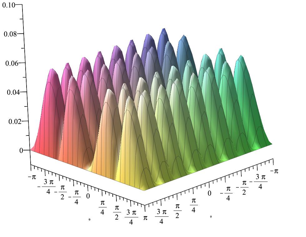
Figure 1: Function $G(\phi,\theta)$.

This function is non-differentiable at $\phi=0,\pm\pi/2,\pm\pi$ and $\theta=0,\pm\pi/2,\pm\pi$. See the standard cusps $\phi^{1/3}$ and $\theta^{1/3}$ on the plots of this function, see Fig.2 below

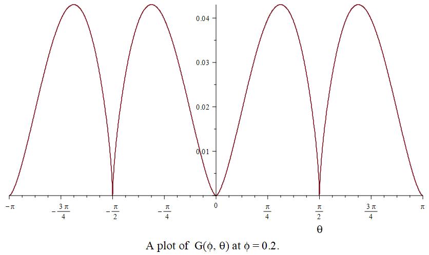
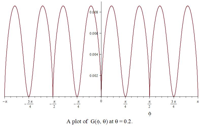
Figure 2: Sections of function $G(\phi,\theta)$.

The trajectories never reach these values, so the sphere is divided into chambers with independent of each other geodesic trajectories.

We have not here integrable systems on the sphere with sextic invariant and smooth metric, see discussion in [3]. We have only a set of smooth trajectories living in the chambers on the sphere.

4.2 Gaffet system on ellipsoid and hyperboloid

All the expressions for integrals of motion can be directly transferred to the ellipsoid and hyperboloid cases without any additional calculations. Indeed, substituting $(y,L)$-variables instead $(x,J)$-variables we obtain integrable system with the Hamiltonian

$$H=L_{1}^{2}+L_{2}^{2}+L_{3}^{2}+\frac{a^{2}}{(y_{1}y_{2}y_{3})^{2/3}}+b^{2}\,\frac{y_{2}^{2}+y_{3}^{2}}{(y_{2}^{2}-y_{3}^{2})^{2}}$$

which after transformation

$$a\to a\,(a_{1}a_{2}a_{3})^{1/3}$$

are real functions for any real $a_{i}$

$$H=U(a_{1}p_{1}^{2}+a_{2}p_{2}^{2}+a_{3}p_{3}^{2})-(x_{1}p_{1}+x_{2}p_{2}+x_{3}p_{3})^{2}+\dfrac{a}{(x_{1}^{2}x_{2}^{2}x_{3}^{2})^{1/3}}+\dfrac{b(a_{3}x_{2}^{2}+a_{2}x_{3}^{2})}{(a_{3}x_{2}^{2}-a_{2}x_{3}^{2})^{2}}\,,$$

where $U$ is given by (3.19).

The same substitution to the geodesic Hamiltonian $\tilde{H}$ (4.23) gives rise to the integrable geodesic flow on the ellipsoid or hyperboloid with sextic invariant. In the case of an ellipsoid, we have smooth local geodesic trajectories living in the finite chambers or parts of the ellipsoid surface. In the case of a hyperboloid, additional, more thorough research is required.

5 Appendix: Maupertuis principle

In modern invariant, coordinate-free Hamiltonian mechanics [1, 44], an integrable system is defined as a Lagrangian submanifold in which $n$ parameters are considered as independent and commuting functions on the symplectic manifold. In a generic case, the Lagrangian submanifold depends on $m>n$ parameters and gives rise to a family of $C^{n}_{m}$ integrable systems.

In traditional Hamiltonian mechanics, there are several coordinate-dependent descriptions of such families of integrable systems, and the Maupertuis principle is the oldest of them. Roughly speaking, the Maupertuis or Jacobi-Maupertuis principle says that trajectories of the natural Hamiltonian systems are geodesics for the suitable metrics on configuration space, see [3, 34, 35, 36] and references within.

Let us take the Hamilton function in the so-called natural form

$$H=T+V(q)\,,\qquad T=\sum_{i,j}\mathrm{g}_{ij}(q)\,p_{i}p_{j}\,,$$

where potential $V(q)$ is a function on coordinates $q$ and $c$. Suppose that $H$ commutes with a sum of the homogeneous polynomials of $m$-order in momenta

$$K=\sum_{m=0}^{N}K_{m}$$

where $N$ is an arbitrary integer number and all terms in the polynomial $K$ have the same parity.

From $\{H,K\}=0$ follows that geodesic Hamiltonian

$$\tilde{T}=\sum_{i,j}\tilde{g}_{ij}(q)\,p_{i}p_{j}=\dfrac{T}{h-V}\,,\qquad\tilde{\mathrm{g}}(q)=\frac{\mathrm{g}(q)}{h-V}$$

where $h$ is a constant, commutes $\{\tilde{T},\tilde{K}\}=0$ with a sum of the homogeneous polynomials of $m$-order in momenta

$$\tilde{K}=K_{m}+\tilde{T}K_{m-2}+\tilde{T}^{2}K_{m-4}+\cdots\,.$$

It is a direct sequence of the Euler homogeneous function theorem.

6 Conclusion

We consider affine quadrics in Euclidean space defined by the equality

$$\frac{x_{1}^{2}}{a_{1}}+\cdots+\frac{x_{n}^{2}}{a_{n}}=1$$

involving real parameters $a_{i}$. Associated with parameters $a_{i}$ and $b_{i}$ quadrics are related for each other by affine transformation $x_{i}\to\sqrt{a_{i}/b_{i}}y_{i}$, which can be lifted to canonical transformation on the cotangent bundle $T^{*}R^{n}$. This canonical transformation changes well-known momentum map and yields different realisations of the Poisson bracket on a Lie algebra $e^{*}(n)$ of the Euclidean motion group.

When some $a_{i}<0$ this canonical transformation maps polynomials $H_{1},\ldots,H_{n}$ with the real coefficients to polynomials $H_{1},\ldots,H_{n}$ with the complex coefficients, but polynomials remain independent and in the involution for each other. We can try to get real integrals of motion for the systems on the noncompact hyperboloids starting with known real integrals of motion for the systems on the sphere by using an additional transformations of the coupling constants.

According to [43] there are two natural questions we would like to address in the non-compact case

• Consider a trajectory coming from infinity with, say, some positive $x_{i}$. Will it be rejected back, or will it pass through to infinity with negative $x_{i}$? How many times will it rotate around the hyperboloid?

• Is there an explicit relation between the values of asymptotic velocities at $x_{i}\to\pm\infty$ in terms of the corresponding integrals?

There is also an intermediate case when geodesics stuck spiralling around the neck, see the possible scattering on a picture from [43], see Fig.3:

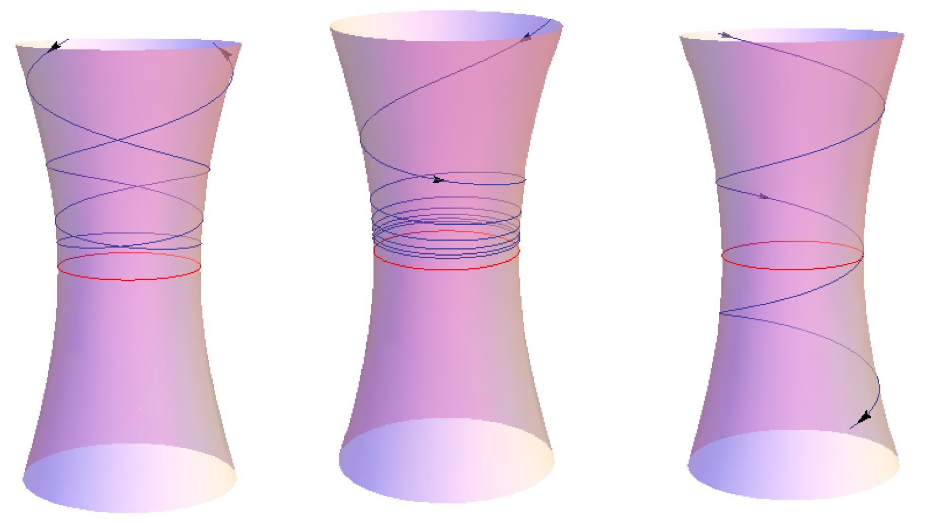
Figure 3: Scattering on the one-sheet hyperboloid from the Veselov and Wu paper.

In this note, we have taken a simple preparatory step to study the problem of geodesic scattering on the hyperboloids associated with such classical problems as Kowalevsky top, Goryachev-Chaplygin top, Goryachev system and other systems on the sphere with the cubic, quartic and sextic invariants.

The work was supported by the Russian Science Foundation (project 21-11-00141).

References

• [1] Arnolโ€™d V. I., Mathematical Methods of Classical Mechanics, Springer-Verlag, New York, second ed., 1989.
• [2] Audin M., Courbes algรฉbriques et systรจmes intรฉgrables: gรฉodรฉsiques des quadriques, Expos. Math., v.12, pp.193-226, 1994.
• [3] Bolsinov, A. V., Kozlov, V. V., Fomenko, A. T., The Maupertuis principle and geodesic flow on the sphere arising from integrable cases in the dynamic of a rigid body, Russian Math. Surv., v.50, no.3, pp.473-501, 1995.
• [4] Borisov A.V., Mamaev I.S., Rigid Body Dynamics, ICS, Izhevsk, 2005.
• [5] Cariรฑena J. F., Raรฑada M. F., Santander M., Superintegrability on the three-dimensional spaces with curvature. Oscillator-related and Kepler-related systems on the sphere $S^{3}$ and on the hyperbolic space $H^{3}$, J. Phys. A: Math. Theor., v.54, 365201, 2021.
• [6] Catoni F., Boccaletti D., Cannata R., Catoni V., Nichelatti E., Zampetti P., The Mathematics of Minkowski Space-Time: With an Introduction to Commutative Hypercomplex Numbers, Birkhรคuser, 2008.
• [7] Davison C. M., Dullin H. R., Bolsinov A. V., Geodesics on the ellipsoid and monodromy, J. Geom. Phys., v.57, no.12, 2007, pp.2437-2454, 2007.
• [8] Dirac, P. A. M., Generalized Hamiltonian dynamics, Canadian Journal of Mathematics, v.2, pp.129-148, 1950.
• [9] Fokas S., Lagerstrรถm P.A., Quadratic and cubic invariants in classical mechanics, J. Math. Anal. Appl., v.74, pp.325-341, 1980.
• [10] Gaffet B., A completely integrable Hamiltonian motion on the surface of a sphere, J. Phys. A: Math. Gen., v.31, pp.1581-1596, 1998.
• [11] Gaffet B., Spinning gas clouds without vorticity: The two missing integrals, J. Phys. A: Math. Gen., v.34, pp. 2087-2095, 2001.
• [12] Goryachev D.N., New cases of a rigid body motion about a fixed point, Warshaw. Univ. Izv., v.3, pp.1-11, 1915.
• [13] Gutierrez-Sagredo I., Herranz F.J., Cayley-Klein Lie Bialgebras: Noncommutative Spaces, Drinfelโ€™d Doubles and Kinematical Applications, Symmetry, v.13, 1249, 2021.
• [14] Herranz F.J., Ballesteros A., Gutiรฉrrez-Sagredo I., Santander M., Cayley-Klein Poisson homogeneous spaces, Twentieth International Conference on Geometry, Integrability and Quantization. June 02-07, 2018, Varna, Bulgaria. Ivaรฏlo M. Mladenov, Vladimir Pulov and Akira Yoshioka, Editors. Avangard Prima, Sofia 2019, pp.161-183, 2019.
• [15] Jacobi C. G. J., Vorlesungen รผber Dynamik, Gesammelte Werke, Supplement Band. Reimer, Berlin, 1884.
• [16] Jovanoviฤ‡ B., The Jacobi-Rosochatius problem on an ellipsoid: The Lax representations and billiards, Arch. Rational Mech. Anal., v.210, pp. 101-131, 2013.
• [17] Kalnins E.G., Willard Miller W., Ye. M. Hakobyan Ye.N., Pogosyan G.S., Superintegrability on the two-dimensional hyperboloid. II, J. Math. Phys., v.40, pp.2291-2306, 1997.
• [18] Katzin H., Levine J., Quadratic first integrals of the geodesic in spaces of constant curvature, Tensor, v.10, p. 97-104, 1965.
• [19] Khudobakhshov V. A., Tsiganov A. V. , Integrable systems on the sphere associated with genus three algebraic curves, Reg. Chaot. Dyn., v.16, pp. 396-414, 2011.
• [20] Knรถrrer H., Geodesics on the ellipsoid, Invent. Math., v.59, no.2, pp.119-143, 1980.
• [21] Knรถrrer H., Geodesics on quadrics and a mechanical problem of C. Neumann., J. Reine Angew. Math., v.334, pp.69-78, 1982.
• [22] Komarov I.V., Kuznetsov V.B., Kowalewskiโ€™s top on the Lie algebras $o(4)$, $e(3)$, $o(3,1)$, J. Phys.A., v.23, pp.841-846, 1990.
• [23] Komarov I.V., Tsiganov A.V., On Classical r-matrix for the Kowalevski gyrostat on so(4), SIGMA, v.2, 12, 9 pages, 2006.
• [24] Kozlov V.V., Some integrable generalizations of the Jacobi problem on geodesics on the ellipsoid, Prikl. Math. Mech. 59, 3-9, 1995.
• [25] Moser J., Geometry of quadrics and spectral theory. In: Chern Symposium 1979, Springer Verlag, Berlin-Heidelberg-New York, pp. 147-188, 1980.
• [26] Moser J., Integrable Hamiltonian systems and spectral theory, Lezioni Fermiane, Pisa, 1981.
• [27] Novikov S.P., Schmelzer I., Periodic solutions of Kirchhoffโ€™s equations for the free motion of a rigid body in a fluid and the extended theory of Lyusternik-Shnirelman- Morse. I., Funct. Anal. Appl., v.15, n0.3, pp.54-66, 1981.
• [28] Sokolov V. V., Tsiganov A. V., Lax pairs for the deformed Kowalevski and Goryachev-Chaplygin tops, Theoret. and Math. Phys., v. 131, no.1, pp.543-549, 2002.
• [29] Struve H., Struve R., Non-euclidean geometries: the Cayley-Klein approach, J. Geom., v. 98, pp. 151-170, 2010.
• [30] Sklyanin E.K., Goryachev-Chaplygin top and the inverse scattering method, J. Math. Sci., v.31, pp.3417-3431, 1985.
• [31] Sommerville D., Classification of Geometries with Projective Metric, Proc. Edinburgh Math. Soc., v.28, pp.25-41, 1909.
• [32] Tabachnikov S. L., Ellipsoids, complete integrability and hyperbolic geometry, Mosc. Math. J., v.2, no.1, pp.183-196, 2002.
• [33] Topalov P. J., Geodesic compatibility and integrability of geodesic flows, J. Math.Phys., v.44, no.2, pp.913-929, 2003.
• [34] Tsiganov A.V., Duality between integrable Stรคckel systems, J. Phys. A: Math. Gen., v.32, pp.7965-7982, 1999.
• [35] A.V. Tsiganov, On an integrable deformation of the spherical top, J. Phys. A: Math. Gen., v.32, p.8355-8363, 1999.
• [36] Tsiganov A.V., The Maupertuis principle and canonical transformation of the extended phase space, J. Nonlinear Math. Phys., v. 8, 157-182, 2001.
• [37] A.V. Tsiganov, On the Kowalevski-Goryachev-Chaplygin gyrostat, J. Phys. A, Math. Gen., v.35, L309-L318, 2002.
• [38] A.V. Tsiganov, On a family of integrable systems on $S^{2}$ with a cubic integral of motion, J. Phys. A: Math. Gen., v.38, p.921-927, 2005.
• [39] Tsiganov A.V., Bรคcklund transformations for the Jacobi system on an ellipsoid, Theoret. and Math. Phys., v.192, n., 1204-1218, 2017.
• [40] Tsiganov A.V., Equivalent integrable metrics on the sphere with quartic invariants, arXiv:2201.09576, 2022.
• [41] Vershilov, A.V., Tsiganov, A.V. On bi-Hamiltonian geometry of some integrable systems on the sphere with cubic integral of motion, J. Phys. A: Math. Theor., v.42:10, 105203, 2009.
• [42] Veselov A.P., Confocal surfaces and integrable billiards on the sphere and in the Lobachevsky space, J. Geom. Phys., v.7, pp.81-107, 1990.
• [43] Veselov A.P., Wu L. H., Geodesic scattering on hyperboloids and Knรถrrerโ€™s map, Nonlinearity, v.34, 5926, 2021.
• [44] Vinogradov A.V., Kupersmidt B.A., The structures of Hamiltonian mechanics, Russ. Math. Surveys, v.32, pp.1747-243, 1977.
• [45] Weierstrass K., รœber die geodรคtischen Linien auf dem dreiachsigen Ellipsoid, in: Mathematische Werke I, pp.257-266, Berlin, Mayer and Mรผller, 1895.
• [46] Yaglom I., Rozenfelโ€™d B. and Yasinskaya E., Projective metrics, Russ. Math. Surv., 1964, 19:5, 49-107, 1964.
• [47] Yaglom I., A Simple Non-Euclidean Geometry and Its Physical Basis, Springer, New York, 1979.
• [48] Yehia H. M., An integrable motion of a particle on a smooth ellipsoid, Reg. Chaot. Dyn., v.8, no.4, pp.463-468, 2003.