Variational and thermodynamically consistent finite element discretization for heat conducting viscous fluids

Evan S. Gawlik   and   François Gay-Balmaz Department of Mathematics, University of Hawai‘i at M$\overline{\mbox{a}}$noa, egawlik@hawaii.eduCNRS - LMD, Ecole Normale Supérieure, francois.gay-balmaz@lmd.ens.fr
Abstract

Respecting the laws of thermodynamics is crucial for ensuring that numerical simulations of dynamical systems deliver physically relevant results. In this paper, we construct a structure-preserving and thermodynamically consistent finite element method and time-stepping scheme for heat conducting viscous fluids. The method is deduced by discretizing a variational formulation for nonequilibrium thermodynamics that extends Hamilton’s principle for fluids to systems with irreversible processes. The resulting scheme preserves the balance of energy and mass to machine precision, as well as the second law of thermodynamics, both at the spatially and temporally discrete levels. The method is shown to apply both with insulated and prescribed heat flux boundary conditions, as well as with prescribed temperature boundary conditions. We illustrate the properties of the scheme with the Rayleigh-Bénard thermal convection. While the focus is on heat conducting viscous fluids, the proposed discrete variational framework paves the way to a systematic construction of thermodynamically consistent discretizations of continuum systems.

1 Introduction

Structure preserving discretization of continuum systems, such as fluids and elastic bodies, is today widely recognized as an essential tool for the construction of numerical schemes when the long time accuracy and the respect of the balance and conservation laws of the simulated system are crucial. Such properties are especially relevant in the context of geophysical fluid dynamics for weather and climate prediction, or in the context of plasma physics.

A well-known constructive approach to deriving such structure preserving discretizations is to exploit the variational formulation underlying the equations of motion. This formulation is deduced from Hamilton’s critical action principle and provides a useful setting for both the temporal and spatial discretization steps. While variational time integrators for finite dimensional systems are today well-established (see [34] and the large series of subsequent works), spatial and spacetime discrete variational approaches for continuum systems are still undergoing foundational developments (e.g. [32, 31, 36, 14, 13, 20]).

Despite their wide range of applicability, a main limitation of variational formulations issued from Hamilton’s principle is their inability to consistently include irreversible processes in the systems. In most of the real world applications of continuum mechanics, however, such processes do have a deep impact on the dynamics. For instance, in the case of fluid dynamics, the processes of heat conduction, diffusion, viscosity, or chemical reactions, play a major role in geophysical, astrophysical, engineering and technological applications. Thermal convection occurring in the planets’ oceans, atmospheres and mantles, as well as in stars, is a typical phenomenon occurring in conjunction with the process of heat transfer among others. Importantly, due to their irreversible character, such phenomena fit into the realm of nonequilibrium thermodynamics, governed by the two laws imposing constraints on the energy and entropy behavior. In order to get reliable and physically meaningful numerical solutions for such systems, it is of paramount importance to preserve these laws at the discrete level, thereby highlighting the need to extend variational discretization from reversible continuum mechanics to nonequilibrium thermodynamics.

We propose in this paper a first step in this direction for the case of fluid dynamics with heat conduction and viscosity. Our approach is based on a variational formulation for nonequilibrium thermodynamics that extends Hamilton’s principle to include irreversibility ([25, 26, 28]). Importantly for the present work, this approach extends to the irreversible setting the well-known variational and geometric formulation of hydrodynamics on diffeomorphism groups initiated in [2]. The resulting class of schemes satisfies the two laws of thermodynamics at the fully discrete level. More precisely, the total energy is shown to be exactly preserved at the fully discrete level when the fluid is adiabatically closed, while a discrete energy balance holds in the presence of external heating. Regarding the second law, the entropy generated by the internal irreversible processes is shown to grow at each time step on each cell.

It turns out that the variational formulation for nonequilibrium thermodynamics yields the equations for heat conducting viscous fluids in a weak form that is quite suitable to achieve thermodynamic consistency and, at the same time, can naturally accommodate both prescribed heat flux (Neumann) or prescribed temperature (Dirichlet) boundary conditions. The variational formulation also naturally involves an internal entropy variable, helping identify the internal entropy production at the fully discrete level, which is well-known to differ from the rate of entropy change in the presence of the entropy flux.

Our paper is structured as follows. In §2 we recall the variational formulation for heat conducting viscous fluids in the insulated case ([26]) and then present the modifications needed for the treatment of a prescribed temperature or prescribed heat flux on the boundary, consistently with the variational formulation of open systems ([28]). We also give the weak formulation of the equations resulting from the variational framework. In §3, following previous works on the reversible case, we carry out this variational formulation on a discrete version of the diffeomorphism group, based on a discontinuous Galerkin discretization of functions. A suitable spatially discrete version of heat conducting viscous flow is obtained for any given discrete fluid Lagrangian. A main subsequent step is the appropriate discretization of the thermodynamic fluxes, which is chosen in accordance with the considered Neumann or Dirichlet boundary conditions, and realized for the Navier-Stokes-Fourier case. It is then shown that the resulting spatial discretization satisfies the two laws of thermodynamics exactly. Thanks to its structure preserving form, the resulting finite element scheme can be followed by an energy preserving time discretization which allows satisfaction of the second law at each step on each fluid cell. Rayleigh-Bénard convection tests are carried out in §4 for both prescribed temperature (Dirichlet) and prescribed heat flux (Neumann) boundary conditions, for several values of Rayleigh numbers, illustrating the predictive value and thermodynamic consistency of our scheme.

2 Variational formulation for heat conducting viscous fluids

We review here the variational formulation of nonequilibrium thermodynamics underlying the structure preserving discretization method that we present for heat conducting viscous fluids. This variational formulation, developed in [25, 26, 28], is an extension of the Hamilton principle which allows one to systematically include irreversible processes in the dynamics, such as friction, viscosity, heat conduction, matter transfer, or chemical reactions. Importantly for the present work, the variational formulation applies to adiabatically closed systems as well as systems exchanging heat and matter with their surroundings [28].

We recall in §2.1 this formulation for heat conducting viscous fluids with insulated boundaries (homogeneous Neumann boundary conditions), and then present the modifications needed for the treatment of a prescribed temperature on the boundary (Dirichlet boundary conditions) or prescribed heat flux at the boundary (nonhomogeneous Neumann boundary conditions), see §2.2. A weak formulation of the equation is deduced from the variational formulation in §2.3 in a unified way for all boundary conditions.

In order to help identify the role and meaning of each variable in a simpler context, both for the adiabatically closed case and for the open case, we present in Appendix A an application of the variational formulation to an elementary finite dimensional example.

2.1 Insulated boundaries

The variational formulation is best expressed in the material (or Lagrangian) description since it is in this description that it is an extension of the Hamilton principle of continuum mechanics and takes its simpler form. The variational formulation in the spatial (or Eulerian) description that underlies our approach is then deduced by using the fluid relabelling symmetry. A finite element spatial discretization of this “Lagrangian-to-Eulerian” variational approach will be developed in §3.

Lagrangian description.

Let $\Omega\subset\mathbb{R}^{d}$, $d=2,3$, be a bounded domain with smooth boundary, $\operatorname{Diff}(\Omega)$ the group of diffeomorphisms of $\Omega$, and $\operatorname{Diff}_{0}(\Omega)$ the subgroup of diffeomorphisms keeping $\partial\Omega$ pointwise fixed. We denote by $\mathcal{F}(\Omega)$ and $\mathcal{F}(\Omega)^{*}$ the spaces of functions and densities on $\Omega$ with sufficient regularity. We identify densities with functions, bearing in mind that the action of $\operatorname{Diff}(\Omega)$ on $\mathcal{F}(\Omega)^{*}$ under this identification differs from the action of $\operatorname{Diff}(\Omega)$ on $\mathcal{F}(\Omega)$; see (6). In the Lagrangian description, the motion of a compressible fluid in the domain $\Omega$ is given by two time dependent maps, the fluid configuration map $\varphi:[t_{0},t_{1}]\rightarrow\operatorname{Diff}_{0}(\Omega)$, giving the position $x=\varphi(t,X)$ at time $t$ of a particle located at $X$ at $t=t_{0}$, and the entropy density $S:[t_{0},t_{1}]\rightarrow\mathcal{F}(\Omega)^{*}$. From mass conservation, the mass density $\varrho_{0}\in\mathcal{F}(\Omega)^{*}$ is constant in time in the Lagrangian description, $\varrho(t,X)=\varrho_{0}(X)$.

In the absence of irreversible processes, the entropy density is also constant in time $S(t,X)=S_{0}(X)$ and the equations of motion follow from the Hamilton principle

$$\delta\int_{t_{0}}^{t_{1}}L(\varphi,\dot{\varphi},S_{0},\varrho_{0}){\rm d}t=0$$ (1)

for variations $\delta\varphi$ with $\delta\varphi|_{t=t_{0},t_{1}}=0$. In (1) the function $L:T\operatorname{Diff}_{0}(\Omega)\times\mathcal{F}(\Omega)^{*}\times\mathcal{F}(\Omega)^{*}\rightarrow\mathbb{R}$ is the Lagrangian of the compressible fluid model, the standard expression being

$$L(\varphi,\dot{\varphi},S,\varrho)=\int_{\Omega}\Big{[}\frac{1}{2}\varrho|\dot{\varphi}|^{2}-\epsilon\big{(}\varrho/J\varphi,S/J\varphi\big{)}-\varrho\phi(\varphi)\Big{]}{\rm d}X$$ (2)

with $J\varphi$ the Jacobian of $\varphi$, $\epsilon$ the internal energy density, and $\phi(x)$ the gravitational potential.

For the heat conducting viscous fluid one also needs to specify the phenomenological expressions of the viscous stress tensor and entropy flux, denoted $P$ and $J_{S}$ in the Lagrangian description. The extension of Hamilton’s principle (1) to heat conducting viscous fluids given in [26] involves two additional variables besides $\varphi(t)\in\operatorname{Diff}_{0}(\Omega)$ and $S(t)\in\mathcal{F}(\Omega)^{*}$: the internal entropy density variable $\Sigma(t)\in\mathcal{F}(\Omega)^{*}$, whose time rate of change is the internal entropy production, and the thermal displacement $\Gamma(t)\in\mathcal{F}(\Omega)$, whose time rate of change is the temperature. The variational principle reads as follows.

Find the curves $\varphi:[t_{0},t_{1}]\rightarrow\operatorname{Diff}_{0}(\Omega)$, $S,\Sigma:[t_{0},t_{1}]\rightarrow\mathcal{F}(\Omega)^{*}$, and $\Gamma:[t_{0},t_{1}]\rightarrow\mathcal{F}(\Omega)$, which are critical for the variational condition

$$\delta\int_{t_{0}}^{t_{1}}\Big{[}L\big{(}\varphi,\dot{\varphi},S,\varrho_{0}\big{)}+\int_{\Omega}(S-\Sigma)\dot{\Gamma}\,{\rm d}X\Big{]}{\rm d}t=0$$ (3)

subject to the phenomenological constraint

$$\frac{\delta L}{\delta S}\dot{\Sigma}=\underbrace{-P:\nabla\dot{\varphi}}_{\text{viscosity}}+\underbrace{J_{S}\cdot\nabla\dot{\Gamma}}_{\text{heat conduction}}$$ (4)

and for variations subject to the variational constraint

$$\frac{\delta L}{\delta S}\delta\Sigma=\underbrace{-P:\nabla\delta\varphi}_{\text{viscosity}}+\underbrace{J_{S}\cdot\nabla\delta\Gamma}_{\text{heat conduction}}$$ (5)

with $\delta\varphi|_{t=t_{0},t_{1}}=\delta\Gamma|_{t=t_{0},t_{1}}=0$, and $\delta\varphi|_{\partial\Omega}=0$. The critical condition of this variational formulation gives the heat conducting viscous fluid equation in the Lagrangian description, see §B.1. In (4) and (5) $\frac{\delta L}{\delta S}$ is the functional derivative of $L$ with respect to $S$, defined as $\left.\frac{d}{d\varepsilon}\right|_{\varepsilon=0}L(\varphi,\dot{\varphi},\varrho,S+\varepsilon\delta S)=\int_{\Omega}\frac{\delta L}{\delta S}\delta S\,{\rm d}X$, for all $\delta S$. It is identified with minus the temperature of the fluid, denoted $\mathfrak{T}=-\frac{\delta L}{\delta S}$ in the Lagrangian description.

Remark 2.1 (Structure of the variational formulation).

The variational formulation (3)–(5) is an extension of the Hamilton principle (1) for fluids which includes two types of constraints: a kinematic (phenomenological) constraint (4) on the critical curve and a variational constraint (5) on the variations to be considered when computing this critical curve. The two constraints are related in a systematic way which formally involves replacing the time rate of changes (here $\dot{\Sigma}$, $\dot{\varphi}$, and $\dot{\Gamma}$) by the $\delta$-variations (here $\delta\Sigma$, $\delta\varphi$, and $\delta\Gamma$). More precisely, on the right hand side of (4) the two terms correspond to the dissipated power density associated to the processes of viscosity and heat conduction, with their virtual version appearing in (5). In coordinates $P:\nabla\dot{\varphi}=P^{A}_{a}\partial_{A}\dot{\varphi}^{a}$ and $J_{S}\cdot\nabla\dot{\Gamma}=(J_{S})^{A}\partial_{A}\dot{\Gamma}$. This setting is common to the variational formulation of adiabatically closed thermodynamic systems [25, 26] and is a nonlinear version of the Lagrange-d’Alembert principle used in nonholonomic mechanics. In Appendix A we recall an application of this type of variational formulation to an elementary finite dimensional thermodynamic system for which the computation of the critical condition is straightforward and which helps explain the role and the meaning of the variables $\Sigma$ and $\Gamma$.

Eulerian description.

We recall here how (3)–(5) can be converted to the Eulerian frame, thereby yielding the variational formulation underlying our structure preserving finite element discretization. The Eulerian versions of the variables $\dot{\varphi},\varrho_{0},S,\Sigma,\Gamma$ are the Eulerian velocity $u$, mass density $\rho$, entropy density $s$, internal entropy density $\varsigma$, and thermal displacement $\gamma$ given as

$\displaystyle u$ $\displaystyle=\dot{\varphi}\circ\varphi^{-1}\in\mathfrak{X}_{0}(\Omega),\qquad\rho=(\varrho_{0}\circ\varphi^{-1})J\varphi^{-1}\in\mathcal{F}(\Omega)^{*},\qquad s=(S\circ\varphi^{-1})J\varphi^{-1}\in\mathcal{F}(\Omega)^{*},$ (6)
$\displaystyle\varsigma$ $\displaystyle=(\Sigma\circ\varphi^{-1})J\varphi^{-1}\in\mathcal{F}(\Omega)^{*},\qquad\gamma=\Gamma\circ\varphi^{-1}\in\mathcal{F}(\Omega),$

where $\mathfrak{X}_{0}(\Omega)=\{u\in\mathfrak{X}(\Omega)\mid u|_{\partial\Omega}=0\}$ is the space of vector fields on $\Omega$ vanishing on the boundary. The Eulerian viscous stress tensor $\sigma$ and entropy flux $j_{s}$ are related to their Lagrangian counterparts $P$ and $J_{S}$ via the Piola transformations

$$\sigma=((P\cdot\nabla\varphi^{\mathsf{T}})\circ\varphi^{-1})J\varphi^{-1}\qquad\text{and}\qquad j_{s}=((\nabla\varphi\cdot J_{S})\circ\varphi^{-1})J\varphi^{-1},$$ (7)

[33]. From its relabelling symmetries, the Lagrangian $L$ can be expressed in terms of the Eulerian variables as $L(\varphi,\dot{\varphi},S,\varrho_{0})=\ell(u,\rho,s)$. For the standard expression given in (2) one gets

$$\ell(u,\rho,s)=\int_{\Omega}\Big{[}\frac{1}{2}\rho|u|^{2}-\epsilon(\rho,s)-\rho\phi\Big{]}{\rm d}x.$$ (8)

With relations (6) and (7), the Eulerian version of the principle (3)–(5) reads as follows. Find the curves $u:[t_{0},t_{1}]\rightarrow\mathfrak{X}_{0}(\Omega)$, $s,\varsigma:[t_{0},t_{1}]\rightarrow\mathcal{F}(\Omega)^{*}$, and $\gamma:[t_{0},t_{1}]\rightarrow\mathcal{F}(\Omega)$, which are critical for the variational condition

$$\delta\int_{t_{0}}^{t_{1}}\Big{[}\ell(u,\rho,s)+\int_{\Omega}(s-\varsigma)D_{t}\gamma\,{\rm d}x\Big{]}{\rm d}t=0,$$ (9)

with the phenomenological constraint and variational constraint given by

$$\frac{\delta\ell}{\delta s}\bar{D}_{t}\varsigma=\underbrace{-\sigma:\nabla u}_{\text{viscosity}}+\underbrace{j_{s}\cdot\nabla(D_{t}\gamma)}_{\text{heat conduction}},$$ (10)
$$\frac{\delta\ell}{\delta s}\bar{D}_{\delta}\varsigma=\underbrace{-\sigma:\nabla v}_{\text{viscosity}}+\underbrace{j_{s}\cdot\nabla(D_{\delta}\gamma)}_{\text{heat conduction}},$$ (11)

and the Euler-Poincaré constraints

$$\delta u=\partial_{t}v+[u,v],\qquad\delta\rho=-\operatorname{div}(\rho v),$$ (12)

see [26] for details. Here $v=\delta\varphi\circ\varphi^{-1}:[t_{0},t_{1}]\rightarrow\mathfrak{X}_{0}(\Omega)$ and $\delta\gamma:[t_{0},t_{1}]\rightarrow\mathcal{F}(\Omega)$ are arbitrary curves with $v|_{t=t_{0},t_{1}}=0$ and $\delta\gamma|_{t=t_{0},t_{1}}=0$, and $\delta s,\delta\varsigma:[t_{0},t_{1}]\rightarrow\mathcal{F}(\Omega)^{*}$. In (9)–(11) we have used the following notations for the Lagrangian derivatives and variations of functions $f$ and densities $g$:

$\displaystyle D_{t}f$ $\displaystyle=\partial_{t}f+u\cdot\nabla f$ $\displaystyle\qquad D_{\delta}f=\delta f+v\cdot\nabla f$ (13)
$\displaystyle\bar{D}_{t}g$ $\displaystyle=\partial_{t}g+\operatorname{div}(gu)$ $\displaystyle\qquad\bar{D}_{\delta}g=\delta g+\operatorname{div}(gv),$

where $v=\delta\varphi\circ\varphi^{-1}$ and $u=\dot{\varphi}\circ\varphi^{-1}$.

By applying the variational principle (9)–(12), we get the equations for a compressible heat conducting viscous fluid with Lagrangian $\ell(u,\rho,s)$

$$\left\{\begin{array}[]{l}\vspace{0.2cm}\displaystyle(\partial_{t}+\pounds_{u})\frac{\delta\ell}{\delta u}=\rho\nabla\frac{\delta\ell}{\delta\rho}+s\nabla\frac{\delta\ell}{\delta s}+\operatorname{div}\sigma\\ \vspace{0.2cm}\displaystyle-\frac{\delta\ell}{\delta s}(\bar{D}_{t}s+\operatorname{div}j_{s})=\sigma\!:\!\nabla u+j_{s}\!\cdot\!\nabla\frac{\delta\ell}{\delta s}\\ \displaystyle\bar{D}_{t}\rho=0,\end{array}\right.$$ (14)

with $\pounds_{u}$ the Lie derivative of one-form densities, together with the conditions

$$D_{t}\gamma=-\frac{\delta\ell}{\delta s},\qquad\bar{D}_{t}\varsigma=\bar{D}_{t}s+\operatorname{div}j_{s},\qquad\text{and}\qquad j_{s}\cdot n=0\;\;\text{on}\;\;\partial\Omega,$$ (15)

see §B.2 for details on the derivation. We have used the functional derivatives of $\ell$, defined as $\left.\frac{d}{d\varepsilon}\right|_{\varepsilon=0}\ell(u+\varepsilon\delta u,\rho,s)=\int_{\Omega}\frac{\delta\ell}{\delta u}\cdot\delta u\,{\rm d}x$, etc. Since $-\frac{\delta\ell}{\delta s}$ is identified with the temperature $T$, the first condition in (15) implies that the variable $\gamma$ is the thermal displacement. From the second condition it follows that $\bar{D}_{t}\varsigma$ is the rate of internal entropy production, which must be positive by the second law of thermodynamics, namely

$$\bar{D}_{t}\varsigma=\bar{D}_{t}s+\operatorname{div}j_{s}\geq 0.$$ (16)

The last condition in (15) is the insulated boundary condition.

We refer to [23, 16, 24] for the use of this type of variational formulation for modelling purposes in nonequilibrium thermodynamics.

Standard Lagrangian.

By using the Lagrangian for Euler fluids given in (8) one gets $\frac{\delta\ell}{\delta u}=\rho u$, $\frac{\delta\ell}{\delta\rho}=\frac{1}{2}|u|^{2}-\frac{\partial\epsilon}{\partial\rho}-\phi$, and $-\frac{\delta\ell}{\delta s}=\frac{\partial\epsilon}{\partial s}=T>0$ the temperature, so that the fluid momentum equation and the entropy equation in (14) take the usual form

$$\rho(\partial_{t}u+u\cdot\nabla u)=-\rho\nabla\phi-\nabla p+\operatorname{div}\sigma,\qquad T(\bar{D}_{t}s+\operatorname{div}j_{s})=\sigma\!:\!\nabla u-j_{s}\!\cdot\!\nabla T$$

with $p=\frac{\partial\epsilon}{\partial\rho}\rho+\frac{\partial\epsilon}{\partial s}s-\epsilon$ the pressure.

Energy and entropy balances.

Defining the total energy $\mathcal{E}=\left\langle\frac{\delta\ell}{\delta u},u\right\rangle-\ell(u,\rho,s)$, from (14) and the boundary conditions $u|_{\partial\Omega}=0$ and $j_{s}\cdot n=0$ we directly get the energy conservation

$$\frac{d}{dt}\mathcal{E}=\int_{\Omega}\operatorname{div}\Big{(}\rho\frac{\delta\ell}{\delta\rho}u+s\frac{\delta\ell}{\delta s}u+\sigma\cdot u+j_{s}\frac{\delta\ell}{\delta s}\Big{)}{\rm d}x=0.$$ (17)

From now on we will focus on the Navier-Stokes-Fourier case with the phenomenological relations

$\displaystyle\sigma=\sigma(u)$ $\displaystyle=2\mu\operatorname{Def}u+\lambda(\operatorname{div}u)\delta,$ with $\mu\geq 0$ and $\zeta=\lambda+\frac{2}{d}\mu\geq 0$ (18)
$\displaystyle j_{s}=j_{s}(T)$ $\displaystyle=-\frac{1}{T}\kappa\nabla T,$ $\displaystyle\text{with $\kappa\geq 0$}.$

Here $\operatorname{Def}u=\frac{1}{2}(\nabla u+\nabla u^{\mathsf{T}})$ is the rate of deformation tensor, $\mu\geq 0$ and $\zeta=\lambda+\frac{2}{d}\mu\geq 0$ are the shear and bulk viscosity coefficients, and $\kappa\geq 0$ is the thermal conductivity coefficient. The signs of the coefficients are imposed by the second law of thermodynamics $\bar{D}_{t}s+\operatorname{div}j_{s}\geq 0$ . Indeed, with (18), the entropy equation reads

$$\bar{D}_{t}s+\operatorname{div}j_{s}=\frac{1}{T}\sigma\!:\!\nabla u-\frac{1}{T}j_{s}\!\cdot\!\nabla T=\frac{2\mu}{T}\left(\operatorname{Def}u\right)^{(0)}\!:\!\left(\operatorname{Def}u\right)^{(0)}+\frac{\zeta}{T}(\operatorname{div}u)^{2}+\frac{\kappa}{T^{2}}|\nabla T|^{2}\geq 0,$$ (19)

where $\left(\operatorname{Def}u\right)^{(0)}$ denotes the trace-free part of $\operatorname{Def}u$. For simplicity, in this paper we will assume that these coefficients are constant.

The discretization that we will develop preserves both the energy conservation (17) and the positivity of the rate of internal entropy production (19).

2.2 Dirichlet boundary conditions

We present here a modification of the variational formulation which allows the treatment of a fluid with prescribed temperature on the boundary $\partial\Omega$.

Lagrangian description.

Since in this case the fluid system is no longer adiabatically closed, the appropriate formulation is found by considering the continuum version of the variational formulation for finite dimensional open thermodynamic systems [28]. This amounts to replacing the constraints (4) and (5) by the kinematic and variational constraints

$$\int_{\Omega}W\frac{\delta L}{\delta S}\dot{\Sigma}\,{\rm d}X=-\int_{\Omega}W\underbrace{(P:\nabla\dot{\varphi})}_{\text{viscosity}}\,{\rm d}X+\int_{\Omega}W\!\!\!\!\underbrace{(J_{S}\cdot\nabla\dot{\Gamma})}_{\text{heat conduction}}\!\!\!\!\,{\rm d}X-\int_{\partial\Omega}W\underbrace{(J_{S}\cdot n)(\dot{\Gamma}-\mathfrak{T}_{0})}_{\text{heat transfer}}\!\,{\rm d}A,\;\forall\;W$$ (20)
$$\int_{\Omega}W\frac{\delta L}{\delta S}\delta\Sigma\,{\rm d}X=-\int_{\Omega}W\underbrace{(P:\nabla\delta\varphi)}_{\text{viscosity}}\,{\rm d}X+\int_{\Omega}W\!\!\!\!\underbrace{(J_{S}\cdot\nabla\delta\Gamma)}_{\text{heat conduction}}\!\!\!\!\,{\rm d}X-\int_{\partial\Omega}W\underbrace{(J_{S}\cdot n)\delta\Gamma}_{\text{heat transfer}}\!\,{\rm d}A,\;\forall\;W,$$ (21)

with $\mathfrak{T}_{0}(X)$ the prescribed temperature on the boundary in the Lagrangian description. When $J_{S}\cdot n=0$ they consistently recover (4) and (5).

We refer to the Appendix A for an application of this type of variational principle for an elementary finite dimensional thermodynamic system exchanging heat with the exterior, which helps the understanding of the new boundary term. In particular, (20) and (21) are continuum versions of the constraints (82) and (83) in Appendix A.

Eulerian description.

Exactly as in §2.1, the variational principle can be converted to the Eulerian description, thereby yielding (9)–(12) with the constraints (10) and (11) replaced by

$$\int_{\Omega}w\frac{\delta\ell}{\delta s}\bar{D}_{t}\varsigma\,{\rm d}x=-\int_{\Omega}w(\sigma:\nabla u)\,{\rm d}x+\int_{\Omega}w(j_{s}\cdot\nabla D_{t}\gamma)\,{\rm d}x-\int_{\partial\Omega}w(j_{s}\cdot n)\left(D_{t}\gamma-T_{0}\right)\,{\rm d}a,\;\forall\;w$$ (22)
$$\int_{\Omega}w\frac{\delta\ell}{\delta s}\bar{D}_{\delta}\varsigma\,{\rm d}x=-\int_{\Omega}w(\sigma:\nabla v)\,{\rm d}x+\int_{\Omega}w(j_{s}\cdot\nabla D_{\delta}\gamma)\,{\rm d}x-\int_{\partial\Omega}w(j_{s}\cdot n)D_{\delta}\gamma\,{\rm d}a,\;\forall\;w.$$ (23)

An application of the variational formulation (9)-(22)-(23)-(12) yields the equations (14) and (15), with the last equation of (15) replaced by

$$(j_{s}\cdot n)(T-T_{0})=0\quad\text{on}\quad\partial\Omega,$$ (24)

see §B.3 for details. With the boundary condition (24), the energy balance (17) is modified as

$$\frac{d}{dt}\mathcal{E}=\int_{\Omega}\operatorname{div}\Big{(}\rho\frac{\delta\ell}{\delta\rho}u+s\frac{\delta\ell}{\delta s}u+\sigma\cdot u+j_{s}\frac{\delta\ell}{\delta s}\Big{)}{\rm d}x=-\int_{\partial\Omega}(j_{s}\cdot n)T_{0}\,{\rm d}a.$$ (25)
Remark 2.2 (Prescribed heat flux).

It is also possible to treat the boundary condition

$$j_{q}\cdot n=q_{0}$$

where $j_{q}=Tj_{s}$ is the heat flux and for some given function $q_{0}:\partial\Omega\rightarrow\mathbb{R}$, which may itself depend on the boundary temperature as $q_{0}(T)$. This is achieved by replacing the last term in (22) with

$$-\int_{\partial\Omega}w\big{(}(j_{s}\cdot n)D_{t}\gamma-q_{0}\big{)}\,{\rm d}a.$$ (26)

The variational constraint (23) is kept unchanged, as it follows from the general variational framework for open systems, see Appendix A. The energy balance now reads

$$\frac{d}{dt}\mathcal{E}=-\int_{\partial\Omega}q_{0}\,{\rm d}a.$$

2.3 Associated weak formulation

The variational derivation presented above yields a weak formulation of the equations and boundary conditions, that will be shown to have a discrete version.

In the absence of irreversible processes, this weak formulation has been derived in [20] and is based on the trilinear forms $a:L^{\infty}(\Omega)^{d}\times H^{1}(\Omega)^{d}\times H^{1}(\Omega)^{d}\to\mathbb{R}$ and $b:L^{2}(\Omega)\times H^{1}(\Omega)\times L^{\infty}(\Omega)^{d}\to\mathbb{R}$ defined by

$\displaystyle a(w,u,v)$ $\displaystyle=-\int_{\Omega}w\cdot[u,v]\,{\rm d}x$
$\displaystyle b(f,\rho,v)$ $\displaystyle=-\int_{\Omega}\rho\nabla f\cdot v\,{\rm d}x.$

For the treatment of the irreversible part, we restrict to the expressions $\sigma=\sigma(u)$ and $j_{s}=j_{s}(T)$ given in (18). For viscosity, we define the trilinear form $c:L^{\infty}(\Omega)\times H^{1}(\Omega)^{d}\times H^{1}(\Omega)^{d}\rightarrow\mathbb{R}$ by

$$c(w,u,v)=\int_{\Omega}w\,\sigma(u):\nabla v\,{\rm d}x.$$ (27)

For heat conduction, we set $F=\{f\in H^{1}(\Omega)\mid 1/f\in L^{\infty}(\Omega),\,\operatorname{div}(\nabla f/f)\in L^{2}(\Omega)\}$ and define $d:W^{1,\infty}(\Omega)\times F\times H^{1}(\Omega)\rightarrow\mathbb{R}$ by

$$d(w,f,g)=\left\{\begin{array}[]{ll}\vspace{0.2cm}\displaystyle\int_{\Omega}w\,j_{s}(f)\cdot\nabla g\,{\rm d}x&\text{for homogeneous Neumann}\\ \displaystyle\int_{\Omega}w\,j_{s}(f)\cdot\nabla g\,{\rm d}x-\int_{\partial\Omega}wj_{s}(f)\cdot ng\,{\rm d}a&\text{for Dirichlet and nonhomogeneous Neumann}\end{array}\right.$$ (28)

and $e:W^{1,\infty}(\Omega)\times F\rightarrow\mathbb{R}$ by

$$e(w,f)=\left\{\begin{array}[]{ll}\vspace{0.2cm}\displaystyle 0&\text{for homogeneous Neumann}\\ \vspace{-0.4cm}\displaystyle\int_{\partial\Omega}wj_{s}(f)\cdot nT_{0}\,{\rm d}a&\text{for Dirichlet}\\ \\ \displaystyle\int_{\partial\Omega}wq_{0}(f)\,{\rm d}a&\text{for nonhomogeneous Neumann}\end{array}\right.$$ (29)

so that the constraints (10)–(11) and (22)–(23) (including the modified version in (26)) can be written in a unified way for all boundary conditions as

$$\Big{\langle}w,\frac{\delta\ell}{\delta s}\bar{D}_{t}\varsigma\Big{\rangle}=-c(w,u,u)+d\Big{(}w,-\frac{\delta\ell}{\delta s},D_{t}\gamma\Big{)}+e\Big{(}w,-\frac{\delta\ell}{\delta s}\Big{)},\quad\forall w$$ (30)

and

$$\Big{\langle}w,\frac{\delta\ell}{\delta s}\bar{D}_{\delta}\varsigma\Big{\rangle}=-c(w,u,v)+d\Big{(}w,-\frac{\delta\ell}{\delta s},D_{\delta}\gamma\Big{)},\quad\forall w,$$ (31)

with $\left\langle\cdot,\cdot\right\rangle$ the $L^{2}$ inner product. Note that the condition $\operatorname{div}(\nabla f/f)\in L^{2}(\Omega)$ was included in the definition of $F$ so that the term $-\int_{\partial\Omega}wj_{s}(f)\cdot ng\,{\rm d}a$ can be given meaning using the identity

$$\int_{\partial\Omega}w\frac{1}{f}\nabla f\cdot ng\,{\rm d}a=\int_{\Omega}\nabla w\cdot\frac{1}{f}(\nabla f)g\,{\rm d}x+\int_{\Omega}w\operatorname{div}\left(\frac{1}{f}\nabla f\right)g\,{\rm dx}+\int_{\Omega}w\frac{1}{f}\nabla f\cdot\nabla g\,{\rm d}x.$$

This condition can be omitted from the definition of $F$ in the homogeneous Neumann setting. Note also that we really have two ways to impose homogeneous Neumann boundary conditions: by choosing $d$ and $e$ as indicated above, or by using the “nonhomogeneous Neumann” $d$ and $e$ with $q_{0}=0$. Both approaches lead to the same equations of motion, but the first approach is slightly simpler, and it simplifies the statement of the second law of thermodynamics below. Therefore we prefer to treat it separately.

Importantly, by using these notations when carrying out the variational formulations (9)–(12) and (9)-(22)-(23)-(12), we get the equations (14), together with the boundary conditions $j_{s}\cdot n=0$ or $(j_{s}\cdot n)(T-T_{0})=0$ in the weak form

$$\left\{\begin{array}[]{l}\displaystyle\vspace{0.2cm}\left\langle\partial_{t}\frac{\delta\ell}{\delta u},v\right\rangle+a\Big{(}\frac{\delta\ell}{\delta u},u,v\Big{)}+b\Big{(}\frac{\delta\ell}{\delta\rho},\rho,v\Big{)}+b\Big{(}\frac{\delta\ell}{\delta s},s,v\Big{)}=-c(1,u,v),\;\forall\,v\\ \displaystyle\vspace{0.2cm}-\left\langle\partial_{t}s,\frac{\delta\ell}{\delta s}w\right\rangle-b\Big{(}\frac{\delta\ell}{\delta s}w,s,u\Big{)}+d\Big{(}1,-\frac{\delta\ell}{\delta s},\frac{\delta\ell}{\delta s}w\Big{)}\\ \displaystyle\vspace{0.2cm}\hskip 113.81102pt=c(w,u,u)+d\Big{(}w,-\frac{\delta\ell}{\delta s},\frac{\delta\ell}{\delta s}\Big{)}-e\Big{(}w,-\frac{\delta\ell}{\delta s}\Big{)},\;\forall\,w\\ \displaystyle\left\langle\partial_{t}\rho,\theta\right\rangle+b(\theta,\rho,u)=0,\;\forall\,\theta,\end{array}\right.$$ (32)

see §B.4 for details. Note in particular the very specific form of the two terms involving $d(\cdot,\cdot,\cdot)$ in the weak form of the entropy equation, which plays a crucial role in our discretization.

With these notations, the energy balance follows as

$\displaystyle\frac{d}{dt}\mathcal{E}$ $\displaystyle=\left\langle\partial_{t}\frac{\delta\ell}{\delta u},u\right\rangle-\left\langle\frac{\delta\ell}{\delta\rho},\partial_{t}\rho\right\rangle-\left\langle\frac{\delta\ell}{\delta s},\partial_{t}s\right\rangle$ (33)
$\displaystyle=-a\Big{(}\frac{\delta\ell}{\delta u},u,u\Big{)}-b\Big{(}\frac{\delta\ell}{\delta\rho},\rho,u\Big{)}-b\Big{(}\frac{\delta\ell}{\delta s},s,u\Big{)}-c(1,u,u)$
$\displaystyle\qquad+b\Big{(}\frac{\delta\ell}{\delta\rho},\rho,u\Big{)}+b\Big{(}\frac{\delta\ell}{\delta s},s,u\Big{)}-d\Big{(}1,-\frac{\delta\ell}{\delta s},\frac{\delta\ell}{\delta s}\Big{)}$
$\displaystyle\qquad+c(1,u,u)+d\Big{(}1,-\frac{\delta\ell}{\delta s},\frac{\delta\ell}{\delta s}\Big{)}-e\Big{(}1,-\frac{\delta\ell}{\delta s}\Big{)}=-e\Big{(}1,-\frac{\delta\ell}{\delta s}\Big{)}$

from the property

$$a(w,u,v)=-a(w,v,u),\;\forall\,u,v,w$$

of the trilinear form $a$.

Conservation of total mass $\int_{\Omega}\rho\,{\rm d}x$ follows from the property

$$b(1,\rho,v)=0,\;\;\forall\rho,v.$$

Regarding entropy production, we have the inequalities $\sigma(u)\!:\!\nabla u\geq 0$ and $-j_{s}(T)\!\cdot\!\nabla T\geq 0$ for all $u$ and all $T>0$, consistently with the second law of thermodynamics written in (16). In terms of $c$, the first condition is equivalently written as

$$c(w,u,u)\geq 0,\;\;\forall\,u,\;\;\forall\,w\geq 0.$$ (34)

For homogeneous Neumann boundary conditions, the second condition is equivalently written as

$$d(w,f,f)\leq 0,\;\;\forall\,f>0,\;\;\forall\,w\geq 0,$$ (35)

while for Dirichlet and nonhomogeneous Neumann boundary conditions, it can be equivalently written as

$$d(w,f,f)\leq 0,\;\;\forall\,f>0,\;\;\forall\,\text{$w\geq 0$, $w$ with compact support in the interior of $\Omega$},$$ (36)

where we recall that the expression for $d$ depends on the boundary condition used. Discrete versions of (34)–(36) will be shown to hold in the discrete case.

Finally, the second law (16) can be equivalently written by using $b$ and $d$ as

$$\left\langle\partial_{t}s,Tw\right\rangle+b(Tw,s,u)-d(1,T,Tw)\geq 0$$ (37)

for all $w\geq 0$ with compact support in $\Omega$.

3 Structure preserving variational discretization

The structure preserving finite element integrator is obtained by developing a discrete version of the variational formulation presented above. In particular, exactly as in the continuous case, the discrete variational formulation of the Eulerian form of the equation is inherited by a variational formulation extending Hamilton’s principle in the Lagrangian description.

This is achieved thanks to the introduction of a discrete version $G_{h}$ of the diffeomorphism group $\operatorname{Diff}(\Omega)$ of fluid motion, acting on discrete functions and densities. We shall follow the approach developed for compressible fluids in [20] based on the earlier works [36, 18, 15, 35, 5]. We refer to [12] for another approach to the variational discretization of (9)–(12) for heat conducting viscous fluids, also based on a discrete version of the diffeomorphism group.

3.1 Discrete setting

Let $\mathcal{T}_{h}$ be a triangulation of $\Omega$. We regard $\mathcal{T}_{h}$ as a member of a family of triangulations parametrized by $h=\max_{K\in\mathcal{T}_{h}}h_{K}$, where $h_{K}=\operatorname{diam}K$ denotes the diameter of a simplex $K$. We assume that this family is shape-regular, meaning that the ratio $\max_{K\in\mathcal{T}_{h}}h_{K}/\rho_{K}$ is bounded above by a positive constant for all $h>0$. Here, $\rho_{K}$ denotes the inradius of $K$.

We shall discretize functions with the discontinuous Galerkin space

$$V_{h}=DG_{q}(\mathcal{T}_{h}):=\{f\in L^{2}(\Omega)\mid f|_{K}\in P_{q}(K),\;\forall\,K\in\mathcal{T}_{h}\}.$$

Considering the discrete diffeomorphism group as a certain subgroup $G_{h}\subset GL(V_{h})$, the action $f\in V_{h}\mapsto gf\in V_{h}$, $g\in G_{h}$ is understood as a discrete analogue of the action $f\in\mathcal{F}(\Omega)\mapsto f\circ\varphi^{-1}\in\mathcal{F}(\Omega)$, $\varphi\in\operatorname{Diff}(\Omega)$, of diffeomorphisms on functions. The discrete analogue of the action $\rho\in\mathcal{F}(\Omega)^{*}\mapsto(\rho\circ\varphi)J\varphi\in\mathcal{F}(\Omega)^{*}$ on densities, written as $\rho\in V_{h}\mapsto\rho\cdot g\in V_{h}$, is defined by $L^{2}$ duality as in the continuous case

$$\left\langle\rho\cdot g,f\right\rangle=\left\langle\rho,gf\right\rangle,\quad\forall f,\rho\in V_{h}.$$ (38)

In particular, the Lagrange-to-Euler relations (6) have the discrete analog

$\displaystyle A$ $\displaystyle=\dot{g}g^{-1},\qquad\rho=\varrho_{0}\cdot g^{-1}\in V_{h},\qquad s=S\cdot g^{-1}\in V_{h},$ (39)
$\displaystyle\varsigma$ $\displaystyle=\Sigma\cdot g^{-1}\in V_{h},\qquad\gamma=g\Gamma\in V_{h}.$

The Lie algebra $\mathfrak{g}_{h}\subset L(V_{h},V_{h})$ of $G_{h}$ acts on discrete functions and densities as $f\in V_{h}\mapsto fA\in V_{h}$ and $\rho\in V_{h}\mapsto\rho\cdot A\in V_{h}$, which satisfy

$$\left\langle\rho\cdot A,f\right\rangle=\left\langle\rho,Af\right\rangle,\quad\forall f,\rho\in V_{h}.$$ (40)

As shown in [20], the realization of elements of this Lie algebra as discrete vector fields is obtained by associating to each $u\in H_{0}(\operatorname{div},\Omega)\cap L^{p}(\Omega)^{d}$ (with $p>2$) the Lie algebra element $A_{u}\in\mathfrak{g}_{h}$ defined by

$$\left\langle A_{u}f,g\right\rangle:=-\sum_{K\in\mathcal{T}_{h}}\int_{K}(\nabla_{u}f)g\,{\rm d}x+\sum_{e\in\mathcal{E}^{0}_{h}}\int_{e}u\cdot\llbracket f\rrbracket\{g\}\,{\rm d}a,\quad\forall f,g\in V_{h},$$

which yields a consistent approximation of the distributional derivative in the direction $u$. Moreover, the linear map $u\in H_{0}(\operatorname{div},\Omega)\cap L^{p}(\Omega)^{d}\mapsto A_{u}\in\mathfrak{g}_{h}$ becomes injective on the Raviart-Thomas finite element space $RT_{2q}(\mathcal{T}_{h})$ [20, Proposition 3.4]. Above, we used the notation $\llbracket f\rrbracket$ and $\{f\}$ for the jump and average of a scalar function $f$ across $e=K_{1}\cap K_{2}\in\mathcal{E}_{h}^{0}$, which are defined by

$$\llbracket f\rrbracket=f_{1}n_{1}+f_{2}n_{2},\quad\{f\}=\frac{1}{2}(f_{1}+f_{2}).$$

Here, $f_{i}=\left.f\right|_{K_{i}}$ and $n_{i}$ is the unit normal vector to $e$ pointing outward from $K_{i}$. Later we will also apply $\{\cdot\}$ to vector fields and interpret it componentwise.

This setting is used in [20] to develop a finite element variational discretization of compressible fluids, by writing the analog to the Hamilton principle (1) on the discrete diffeomorphism group $G_{h}$ and using the first three relations (39) to deduce its Eulerian version. The discrete Lagrangian $\ell_{d}:\mathfrak{g}_{h}\times V_{h}\times V_{h}\rightarrow\mathbb{R}$ can be defined from a given continuous Lagrangian $\ell$ as

$$\ell_{d}(A,\rho,s):=\ell(\widehat{A},\rho,s)$$

thanks to the Lie algebra-to-vector field map $A\in\mathfrak{g}_{h}\mapsto\widehat{A}\in[V_{h}]^{d}$ defined by

$$\widehat{A}:=-\sum_{k=1}^{d}A(\pi_{h}(x^{k}))e_{k},$$

where $x^{k}:\Omega\to\mathbb{R}$ is the $k$th coordinate function, $\{e_{k}\}_{k=1}^{d}$ is the standard basis for $\mathbb{R}^{d}$, and $\pi_{h}:L^{2}(\Omega)\rightarrow V_{h}$ the $L^{2}$-orthogonal projector, which we interpret componentwise when applied to a vector field. It satisfies $\widehat{A_{u}}=\pi_{h}(u)$.

3.2 Discrete variational formulation

We discretize the velocity by using the continuous Galerkin space

$$U_{h}^{\rm grad}=CG_{r}(\mathcal{T}_{h})^{d}:=\{u\in H^{1}_{0}(\Omega)^{d}\mid u|_{K}\in P_{r}(K)^{d},\;\forall\,K\in\mathcal{T}_{h}\}.$$

Assuming $r\leq q$ (see Remark 3.1 for $r>q$), we denote by $\Delta_{h}\subset\mathfrak{g}_{h}$ the subspace corresponding to $U_{h}^{\rm grad}$ via the injective map $u\mapsto A_{u}$. We denote by $\pi_{h}^{\rm grad}:L^{2}(\Omega)^{d}\to U_{h}^{\rm grad}$ the $L^{2}$-orthogonal projector onto $U_{h}^{\rm grad}$.

Consider discretizations of $d$ and $e$ given as $d_{h}:V_{h}\times V_{h}\times V_{h}\rightarrow\mathbb{R}$ and $e_{h}:V_{h}\times V_{h}\rightarrow\mathbb{R}$. For now, we only suppose that $d_{h}$ is linear in its first and third arguments, and $e_{h}$ is linear in its first argument. The explicit form and their properties are stated later.

With this setting, the discrete version of the variational formulation (9)-(30)-(31)-(12) reads as follows. Find $A:[t_{0},t_{1}]\rightarrow\Delta_{h}$ and $\rho,s,\varsigma,\gamma:[t_{0},t_{1}]\rightarrow V_{h}$ which are critical for the variational condition

$$\delta\int_{t_{0}}^{t_{1}}\Big{[}\ell_{d}(A,\rho,s)+\langle s-\varsigma,D_{t}^{h}\gamma\rangle\Big{]}\,{\rm d}t=0,$$ (41)

with the phenomenological constraint and variational constraint given by

$$\left\langle\frac{\delta\ell_{d}}{\delta s}\bar{D}_{t}^{h}\varsigma,w\right\rangle=-c(w,\widehat{A},\widehat{A})+d_{h}\left(w,-\frac{\delta\ell_{d}}{\delta s},D_{t}^{h}\gamma\right)+e_{h}\left(w,-\frac{\delta\ell_{d}}{\delta s}\right),\quad\forall w\in V_{h},$$ (42)
$$\left\langle\frac{\delta\ell_{d}}{\delta s}\bar{D}_{\delta}^{h}\varsigma,w\right\rangle=-c(w,\widehat{A},\widehat{B})+d_{h}\left(w,-\frac{\delta\ell_{d}}{\delta s},D_{\delta}^{h}\gamma\right),\quad\forall w\in V_{h},$$ (43)

and with Euler-Poincaré variations

$\displaystyle\delta A$ $\displaystyle=\partial_{t}B+[B,A],$ (44)
$\displaystyle\delta\rho$ $\displaystyle=-\rho\cdot B,$ (45)

for $B(t)$ an arbitrary curve in $\Delta_{h}$ with $B(0)=B(T)=0$, and with $\delta\gamma|_{t=0,T}=0$.

Above we have defined the discrete analogues to the Lagrangian time derivatives and variations considered in (13) as

$\displaystyle D_{t}^{h}f$ $\displaystyle=\partial_{t}f-Af$ $\displaystyle\quad D_{\delta}^{h}f=\delta f-Bf$ (46)
$\displaystyle\bar{D}_{t}^{h}\rho$ $\displaystyle=\partial_{t}\rho+\rho\cdot A$ $\displaystyle\quad\bar{D}_{\delta}^{h}\rho=\delta\rho+\rho\cdot B.$

In (42) and (43), the partial derivative $\frac{\delta\ell_{d}}{\delta s}\in V_{h}$ is defined exactly as in the continuous case, with respect to the $L^{2}$ duality pairing on $V_{h}$.

Proposition 3.1.

The equations of motion that result from (41)–(43) and from the definition $\rho=\varrho_{0}\cdot g^{-1}$ are

$$\left\{\begin{array}[]{l}\vspace{0.2cm}\displaystyle\left\langle\partial_{t}\frac{\delta\ell}{\delta u},v\right\rangle+a_{h}\Big{(}\pi_{h}\frac{\delta\ell}{\delta u},u,v\Big{)}+b_{h}\Big{(}\pi_{h}\frac{\delta\ell}{\delta\rho},\rho,v\Big{)}\\ \displaystyle\vspace{0.2cm}\hskip 113.81102pt+b_{h}\Big{(}\pi_{h}\frac{\delta\ell}{\delta s},s,v\Big{)}=-c(1,u,v),\;\;\forall\,v\in U_{h}^{\rm grad},\\ \vspace{0.2cm}\displaystyle\left\langle\partial_{t}\rho,\theta\right\rangle+b_{h}(\theta,\rho,u)=0,\;\;\forall\,\theta\in V_{h},\\ \vspace{0.2cm}\displaystyle-\left\langle\partial_{t}s,\pi_{h}\Big{(}\frac{\delta\ell}{\delta s}\Big{)}w\right\rangle-b_{h}\Big{(}\pi_{h}\Big{(}\pi_{h}\Big{(}\frac{\delta\ell}{\delta s}\Big{)}w\Big{)},s,u\Big{)}+d_{h}\Big{(}1,-\pi_{h}\frac{\delta\ell}{\delta s},\pi_{h}\Big{(}\pi_{h}\Big{(}\frac{\delta\ell}{\delta s}\Big{)}w\Big{)}\Big{)}\\ \displaystyle\vspace{0.2cm}\hskip 85.35826pt=c(w,u,u)+d_{h}\Big{(}w,-\pi_{h}\frac{\delta\ell}{\delta s},\pi_{h}\frac{\delta\ell}{\partial s}\Big{)}-e_{h}\Big{(}w,-\pi_{h}\frac{\delta\ell}{\delta s}\Big{)},\;\;\forall\,w\in V_{h},\end{array}\right.$$ (47)

where

$\displaystyle a_{h}(w,u,v)$ $\displaystyle=-\int_{\Omega}\widehat{A_{w}}\cdot\widehat{[A_{u},A_{v}]}\,{\rm d}x=-\int_{\Omega}w\cdot[u,v]\,{\rm d}x$ (48)
$\displaystyle b_{h}(f,\rho,u)$ $\displaystyle=\langle\rho,A_{u}f\rangle=-\sum_{K\in\mathcal{T}_{h}}\int_{K}(\nabla_{u}f)\rho\,{\rm d}x+\sum_{e\in\mathcal{E}^{0}_{h}}\int_{e}u\cdot\llbracket f\rrbracket\{\rho\}\,{\rm d}a.$ (49)

The variational principle (41)–(43) also yields the conditions

$$D^{h}_{t}\gamma=-\pi_{h}\frac{\delta\ell}{\delta s},\qquad\Big{\langle}\bar{D}_{t}^{h}(\varsigma-s),\delta\gamma\Big{\rangle}=-d_{h}\Big{(}1,-\pi_{h}\frac{\delta\ell}{\delta s},\delta\gamma\Big{)},\;\forall\,\delta\gamma\in V_{h}.$$ (50)
Remark 3.1.

The second equality in (48) is valid if $r\leq q$. If $r>q$, then we can still arrive at the same scheme by considering a discrete diffeomorphism group $G_{h}\subset GL(DG_{r}(\mathcal{T}_{h}))$ and treating $\rho,s,\varsigma,\gamma$ as elements of $DG_{q}(\mathcal{T}_{h})\subset DG_{r}(\mathcal{T}_{h})$; see [20, Remark 5.1]. In both cases, the fact that our discrete velocity field is continuous is important. In the absence of continuity, the formula (48) contains additional terms involving jumps across codimension-1 faces; see [20, Proposition 4.3]. The absence of these jump terms renders $a_{h}$ independent of $h$, so we drop the subscript $h$ in what follows.

Remark 3.2.

Note that (49) is a standard discontinuous Galerkin discretization of the scalar advection operator, see [8].

Proof.

Taking the variations in (41) yields

$\displaystyle\int_{t_{0}}^{t_{1}}\Big{[}\Big{\langle}\!\!\Big{\langle}\frac{\delta\ell_{d}}{\delta A},\delta A\Big{\rangle}\!\!\Big{\rangle}+\Big{\langle}\frac{\delta\ell_{d}}{\delta\rho},\delta\rho\Big{\rangle}+\Big{\langle}\frac{\delta\ell_{d}}{\delta s},\delta s\Big{\rangle}+\Big{\langle}\delta s,D_{t}^{h}\gamma\Big{\rangle}-\Big{\langle}\delta\varsigma,D_{t}^{h}\gamma\Big{\rangle}$ (51)
$\displaystyle\qquad\qquad\qquad-\Big{\langle}\bar{D}_{t}^{h}(s-\varsigma),\delta\gamma\Big{\rangle}-\Big{\langle}s-\varsigma,\delta A\gamma\Big{\rangle}\Big{]}{\rm d}t=0,$

where $\big{\langle}\!\big{\langle}\cdot,\cdot\big{\rangle}\!\big{\rangle}:\mathfrak{g}_{h}^{*}\times\mathfrak{g}_{h}\to\mathbb{R}$ denotes the duality pairing on $\mathfrak{g}_{h}^{*}\times\mathfrak{g}_{h}$. We used $\int_{t_{0}}^{t_{1}}\left\langle s-\varsigma,D_{t}^{h}\delta\gamma\right\rangle{\rm d}t=-\int_{t_{0}}^{t_{1}}\left\langle\bar{D}_{t}^{h}(s-\varsigma),\delta\gamma\right\rangle{\rm d}t$ which follows from (40), (46), and $\delta{\gamma}|_{t=t_{0},t_{1}}=0$. Since $\delta s$ is arbitrary in $V_{h}$, we get the condition

$$D_{t}^{h}\gamma=-\frac{\delta\ell_{d}}{\delta s}.$$ (52)

Making use of this condition and using (43) yields

$\displaystyle\int_{t_{0}}^{t_{1}}\Big{[}\Big{\langle}\!\!\Big{\langle}\frac{\delta\ell_{d}}{\delta A},\delta A\Big{\rangle}\!\!\Big{\rangle}+\Big{\langle}\frac{\delta\ell_{d}}{\delta\rho},\delta\rho\Big{\rangle}-c(1,\widehat{A},\widehat{B})+d_{h}\Big{(}1,-\frac{\delta\ell_{d}}{\delta s},D_{\delta}^{h}\gamma\Big{)}$
$\displaystyle\qquad\qquad\qquad\qquad-\Big{\langle}\frac{\delta\ell_{d}}{\delta s},\varsigma\cdot B\Big{\rangle}-\Big{\langle}\bar{D}_{t}^{h}(s-\varsigma),\delta\gamma\Big{\rangle}-\Big{\langle}s-\varsigma,\delta A\gamma\Big{\rangle}\Big{]}{\rm d}t=0.$

Using that $\delta\gamma$ is arbitrary and independent of the other variations, we get

$$\Big{\langle}\bar{D}_{t}^{h}(\varsigma-s),\delta\gamma\Big{\rangle}=-d_{h}\Big{(}1,-\frac{\delta\ell_{d}}{\delta s},\delta\gamma\Big{)},\;\;\forall\,\delta\gamma\in V_{h}.$$ (53)

With this, the previous condition becomes

$$\int_{t_{0}}^{t_{1}}\Big{[}\Big{\langle}\!\!\Big{\langle}\frac{\delta\ell_{d}}{\delta A},\delta A\Big{\rangle}\!\!\Big{\rangle}-\Big{\langle}s-\varsigma,\delta A\gamma\Big{\rangle}-\Big{\langle}\frac{\delta\ell_{d}}{\delta\rho},\rho\cdot B\Big{\rangle}-\Big{\langle}\frac{\delta\ell_{d}}{\delta s},\varsigma\cdot B\Big{\rangle}-c(1,\widehat{A},\widehat{B})-d_{h}\Big{(}1,-\frac{\delta\ell_{d}}{\delta s},B\gamma\Big{)}\Big{]}{\rm d}t=0.$$

Using $\delta A=\partial_{t}B+[B,A]$ and the computation

$\displaystyle\int_{t_{0}}^{t_{1}}\left\langle s-\varsigma,\delta A\gamma\right\rangle{\rm d}t=\int_{t_{0}}^{t_{1}}\left\langle s-\varsigma,(\partial_{t}B+[B,A])\gamma\right\rangle{\rm d}t$
$\displaystyle=\int_{t_{0}}^{t_{1}}\left\langle-\partial_{t}(s-\varsigma),B\gamma\right\rangle-\left\langle s-\varsigma,B\partial_{t}\gamma\right\rangle+\left\langle(s-\varsigma)\cdot B,A\gamma\right\rangle-\left\langle(s-\varsigma)\cdot A,B\gamma\right\rangle{\rm d}t$
$\displaystyle=\int_{t_{0}}^{t_{1}}\left\langle-\bar{D}^{h}_{t}(s-\varsigma),B\gamma\right\rangle-\Big{\langle}(s-\varsigma)\cdot B,D^{h}_{t}\gamma\Big{\rangle}{\rm d}t$
$\displaystyle=\int_{t_{0}}^{t_{1}}-d_{h}\Big{(}1,-\frac{\delta\ell_{d}}{\delta s},B\gamma\Big{)}+\Big{\langle}(s-\varsigma)\cdot B,\frac{\delta\ell_{d}}{\delta s}\Big{\rangle}{\rm d}t,$

the previous condition becomes

$$\int_{0}^{T}\Big{[}\Big{\langle}\!\!\Big{\langle}-\partial_{t}\frac{\delta\ell_{d}}{\delta A},B\Big{\rangle}\!\!\Big{\rangle}+\Big{\langle}\!\!\Big{\langle}\frac{\delta\ell_{d}}{\delta A},[B,A]\Big{\rangle}\!\!\Big{\rangle}-\Big{\langle}\frac{\delta\ell_{d}}{\delta\rho},\rho\cdot B\Big{\rangle}-\Big{\langle}\frac{\delta\ell_{d}}{\delta s},s\cdot B\Big{\rangle}-c(1,\widehat{A},\widehat{B})\Big{]}{\rm d}t=0.$$

Using that $A\in\Delta_{h}$ means $A=A_{u}$ for $u\in U^{\rm grad}_{h}$ and using the definitions of $a$ and $b_{h}$ in (48) and (49), together with $\frac{\delta\ell_{d}}{\delta\rho}=\pi_{h}\frac{\delta\ell}{\delta\rho}$, $\frac{\delta\ell_{d}}{\delta s}=\pi_{h}\frac{\delta\ell}{\delta s}$, and $\Big{\langle}\!\!\Big{\langle}\frac{\delta\ell_{d}}{\delta A_{u}},C\Big{\rangle}\!\!\Big{\rangle}=\left\langle\pi_{h}\frac{\delta\ell}{\delta u},\widehat{C}\right\rangle$, we get the first equations of (47).

Combining the constraint (42) and condition (52), we get

$$\Big{\langle}\bar{D}_{t}^{h}\varsigma,\pi_{h}\Big{(}\frac{\delta\ell_{d}}{\delta s}w\Big{)}\Big{\rangle}=-c(w,\widehat{A},\widehat{A})-d_{h}\Big{(}w,-\frac{\delta\ell_{d}}{\delta s},\frac{\delta\ell_{d}}{\delta s}\Big{)}+e_{h}\Big{(}w,-\frac{\delta\ell_{d}}{\delta s}\Big{)},\quad\forall w\in V_{h}.$$

Using (53) and $A=A_{u}$ this becomes

$$\Big{\langle}\bar{D}_{t}^{h}s,\pi_{h}\Big{(}\frac{\delta\ell_{d}}{\delta s}w\Big{)}\Big{\rangle}-d_{h}\Big{(}1,-\frac{\delta\ell_{d}}{\delta s},\pi_{h}\Big{(}\frac{\delta\ell_{d}}{\delta s}w\Big{)}\Big{)}=-c(w,u,u)-d_{h}\Big{(}w,-\frac{\delta\ell_{d}}{\delta s},\frac{\delta\ell_{d}}{\delta s}\Big{)}+e_{h}\Big{(}w,-\frac{\delta\ell_{d}}{\delta s}\Big{)},$$

$\forall w\in V_{h}$. We have thus derived the entropy equation in (47). The mass density equation readily follows from $\rho=\varrho_{0}\cdot g^{-1}$ while the conditions (50) have been obtained in (52) and (53). ∎

Energy balance and mass conservation.

The exact same proof as in the continuous case works, see (33), giving energy balance and mass conservation in the spatially discrete setting as

$\displaystyle\frac{d}{dt}\mathcal{E}$ $\displaystyle=-e_{h}\Big{(}1,-\pi_{h}\frac{\delta\ell}{\delta s}\Big{)}$ (54)
$\displaystyle\frac{d}{dt}\int_{\Omega}\rho\,{\rm d}x$ $\displaystyle=0.$ (55)
Remark 3.3.

The conservation properties above continue to hold if we omit the outermost projection $\pi_{h}$ from the terms of the form $\pi_{h}\Big{(}\pi_{h}\Big{(}\frac{\delta\ell}{\delta s}\Big{)}w\Big{)}$ in (47). They also continue to hold if we omit the $\pi_{h}$ from $\pi_{h}\frac{\delta\ell}{\delta u}$ in (47). We find it advantageous to make these modifications, since they simplify the implementation of the scheme. We do not omit the $\pi_{h}$ from $\pi_{h}\frac{\delta\ell}{\delta\rho}$, since this interferes with the balance of energy. Likewise, we do not omit the $\pi_{h}$ from $\pi_{h}\frac{\delta\ell}{\delta s}$, since we have found that the time-discrete version of (47) is difficult to solve numerically without it; Newton’s method converges much more reliably when the projection is present.

In summary, we solve

$$\!\!\left\{\begin{array}[]{l}\vspace{0.2cm}\displaystyle\left\langle\partial_{t}\frac{\delta\ell}{\delta u},v\right\rangle+a\Big{(}\frac{\delta\ell}{\delta u},u,v\Big{)}+b_{h}\Big{(}\pi_{h}\frac{\delta\ell}{\delta\rho},\rho,v\Big{)}-b_{h}(T,s,v)=-c(1,u,v),\;\;\forall\,v\in U_{h}^{\rm grad},\\ \vspace{0.2cm}\displaystyle\left\langle\partial_{t}\rho,\theta\right\rangle+b_{h}(\theta,\rho,u)=0,\;\;\forall\,\theta\in V_{h},\\ \vspace{0.2cm}\displaystyle\left\langle\partial_{t}s,Tw\right\rangle+b_{h}(Tw,s,u)-d_{h}(1,T,Tw)=c(w,u,u)-d_{h}(w,T,T)-e_{h}(w,T),\;\;\forall\,w\in V_{h},\end{array}\right.$$ (56)

where $T=-\frac{\delta\ell_{d}}{\delta s}=-\pi_{h}\frac{\delta\ell}{\delta s}$.

3.3 Discretization of thermodynamic fluxes

We now discuss our discretizations $d_{h}$ and $e_{h}$ of the maps $d$ and $e$ defined in (28) and (29). We will design $d_{h}$ and $e_{h}$ so that the discrete entropy equation

$$\langle\partial_{t}s,Tw\rangle+b_{h}(Tw,s,u)-d_{h}(1,T,Tw)=c(w,u,u)-d_{h}(w,T,T)-e_{h}(w,T),\quad\forall w\in V_{h}$$ (57)

yields a consistent discretization of the continuous entropy equation

$$T(\bar{D}_{t}s+\operatorname{div}j_{s})=\sigma:\nabla u-j_{s}\cdot\nabla T.$$

We restrict our attention to the setting where $j_{s}=j_{s}(T)=-\frac{1}{T}\kappa\nabla T$, so that the above equation simplifies to

$$T\bar{D}_{t}s-\sigma:\nabla u=\kappa\Delta T.$$

Note that an integration by parts shows that the exact solution $(u,\rho,s,T)$ of the continuous problem satisfies

$$\langle\partial_{t}s,Tw\rangle+b_{h}(Tw,s,u)-c(w,u,u)=\langle T\bar{D}_{t}s-\sigma:\nabla u,w\rangle,\quad\forall w\in V_{h}.$$

Thus, to ensure consistency, we aim to design $d_{h}$ and $e_{h}$ so that the exact solution also satisfies

$$d_{h}(1,T,Tw)-d_{h}(w,T,T)-e_{h}(w,T)=\langle\kappa\Delta T,w\rangle,\quad\forall w\in V_{h}.$$ (58)

Our discussion is split into three cases: homogeneous Neumann boundary conditions on $T$, Dirichlet boundary conditions on $T$, and nonhomogneous Neumann boundary conditions on $T$. To simplify the discussion, we consider the setting where (57) is implemented with $T=-\frac{\delta\ell}{\delta s}$. The case in which one uses $T=-\pi_{h}\frac{\delta\ell}{\delta s}$ is addressed in Remark 3.4.

Homogeneous Neumann boundary conditions.

In this case we set $e_{h}=0$ and discretize $d$ with

$$\begin{split}d_{h}(w,f,g)&=-\sum_{K\in\mathcal{T}_{h}}\int_{K}\frac{w}{f}\kappa\nabla f\cdot\nabla g\,{\rm d}x+\sum_{e\in\mathcal{E}_{h}^{0}}\int_{e}\frac{1}{\{f\}}\{w\kappa\nabla f\}\cdot\llbracket g\rrbracket\,{\rm d}a\\ &\qquad-\sum_{e\in\mathcal{E}_{h}^{0}}\int_{e}\frac{1}{\{f\}}\{w\kappa\nabla g\}\cdot\llbracket f\rrbracket\,{\rm d}a-\sum_{e\in\mathcal{E}_{h}^{0}}\frac{\eta}{h_{e}}\int_{e}\frac{\{w\}}{\{f\}}\llbracket f\rrbracket\cdot\llbracket g\rrbracket\,{\rm d}a,\end{split}$$ (59)

where $\eta>0$ is a penalty parameter. This is a standard non-symmetric interior penalty discretization of $-\int_{\Omega}\kappa\nabla f\cdot\nabla g\,{\rm d}x$ [7, Section 10.5], generalized to incorporate the weight $w/f$ appearing in $d(w,f,g)=-\int_{\Omega}\frac{w}{f}\kappa\nabla f\cdot\nabla g\,dx$. Using the identity $\llbracket fg\rrbracket=\llbracket f\rrbracket\{g\}+\{f\}\llbracket g\rrbracket$, a few calculations show that for every $w,T\in V_{h}$,

$\displaystyle d_{h}(1,T,Tw)-d_{h}(w,T,T)$ (60)
$\displaystyle=-\sum_{K\in\mathcal{T}_{h}}\int_{K}\kappa\nabla T\cdot\nabla w\,{\rm d}x+\sum_{e\in\mathcal{E}_{h}^{0}}\int_{e}\{\kappa\nabla T\}\cdot\llbracket w\rrbracket\,{\rm d}a-\sum_{e\in\mathcal{E}_{h}^{0}}\int_{e}\kappa(\{\nabla w\}+\varepsilon)\cdot\llbracket T\rrbracket\,{\rm d}a$
$\displaystyle\quad-\sum_{e\in\mathcal{E}_{h}^{0}}\frac{\eta}{h_{e}}\int_{e}\llbracket T\rrbracket\cdot\llbracket w\rrbracket\,{\rm d}a,$

where

$$\varepsilon=\frac{1}{\{T\}}\left(\{\nabla(Tw)\}-\{\nabla T\}\{w\}-\{T\}\{\nabla w\}\right).$$ (61)

Hence, for smooth $T$, we get

$$d_{h}(1,T,Tw)-d_{h}(w,T,T)-e_{h}(w,T)=\int_{\Omega}\kappa\Delta Tw\,{\rm d}x-\int_{\partial\Omega}\kappa\nabla T\cdot nw\,{\rm d}a,\quad\forall w\in V_{h}.$$ (62)

This shows that the method is consistent: The exact solution (with homogeneous Neumann boundary conditions on $T$) satisfies (58) (where here $e_{h}=0$). Furthermore, the presence of $\int_{\partial\Omega}\nabla T\cdot nw\,{\rm d}a$ in (62) shows that the scheme enforces homogeneous Neumann boundary conditions on $T$ in a natural way.

We also have for every $w,T\in V_{h}$,

$$d_{h}(w,T,T)=-\sum_{K\in\mathcal{T}_{h}}\int_{K}\frac{w}{T}\kappa|\nabla T|^{2}\,{\rm d}x-\sum_{e\in\mathcal{E}_{h}^{0}}\frac{\eta}{h_{e}}\int_{e}\frac{\{w\}}{\{T\}}|\llbracket T\rrbracket|^{2}\,{\rm d}a,$$ (63)

so the following inequality holds:

$$d_{h}(w,T,T)\leq 0,\;\;\forall\;T>0,\;\;\forall\;w\geq 0,\qquad T,w\in V_{h}.$$ (64)

This is the discrete version of the thermodynamic consistency condition (35). In particular, $d_{h}(1_{K},T,T)\leq 0$, for all $K$, where $1_{K}$ denotes the indicator function for $K$.

Dirichlet boundary conditions.

Next we consider Dirichlet boundary conditions. To distinguish the choice of $d_{h}$ above from the forthcoming choice, we denote the former by $d_{h}^{N}$ and the latter by $d_{h}^{D}$, and similarly for $e_{h}$. We define

$$e_{h}^{D}(w,f)=-\int_{\partial\Omega}\frac{w}{f}\kappa\nabla f\cdot nT_{0}\,{\rm d}a+\sum_{e\in\mathcal{E}_{h}^{\partial}}\frac{\eta}{h_{e}}\int_{e}w(f-T_{0})\,{\rm d}a$$ (65)

and

$$\begin{split}d_{h}^{D}(w,f,g)&=-\sum_{K\in\mathcal{T}_{h}}\int_{K}\frac{w}{f}\kappa\nabla f\cdot\nabla g\,{\rm d}x+\sum_{e\in\mathcal{E}_{h}^{0}}\int_{e}\frac{1}{\{f\}}\{w\kappa\nabla f\}\cdot\llbracket g\rrbracket\,{\rm d}a-\sum_{e\in\mathcal{E}_{h}^{0}}\int_{e}\frac{1}{\{f\}}\{w\kappa\nabla g\}\cdot\llbracket f\rrbracket\,{\rm d}a\\ &\quad-\sum_{e\in\mathcal{E}_{h}^{0}}\frac{\eta}{h_{e}}\int_{e}\frac{\{w\}}{\{f\}}\llbracket f\rrbracket\cdot\llbracket g\rrbracket\,{\rm d}a-\sum_{e\in\mathcal{E}_{h}^{\partial}}\int_{e}\frac{w}{f}\kappa\nabla g\cdot n(f-T_{0})\,{\rm d}a+\sum_{e\in\mathcal{E}_{h}^{\partial}}\int_{e}\frac{w}{f}\kappa\nabla f\cdot ng\,{\rm d}a,\end{split}$$ (66)

where $T_{0}:\partial\Omega\rightarrow\mathbb{R}$ is the prescribed temperature on the boundary. Like (59), (66) is a standard non-symmetric interior penalty discretization of $-\int_{\Omega}\kappa\nabla f\cdot\nabla g\,{\rm d}x$ (this time for problems with Dirichlet boundary conditions), generalized to incorporate the weight $w/f$ appearing in $d(w,f,g)=-\int_{\Omega}\frac{w}{f}\kappa\nabla f\cdot\nabla g\,{\rm d}x+\int_{\partial\Omega}\frac{w}{f}\kappa\nabla f\cdot ng\,{\rm d}a$, see (28). It is related to (59) via the addition of three boundary terms:

  1. 1.

    A term $\sum_{e\in\mathcal{E}_{h}^{\partial}}\int_{e}\frac{w}{f}\kappa\nabla f\cdot ng\,{\rm d}a$ that corresponds to the term $-\int_{\partial\Omega}wj_{s}(f)\cdot ng\,{\rm d}a$ appearing in (28).

  2. 2.

    A term $-\sum_{e\in\mathcal{E}_{h}^{\partial}}\int_{e}\frac{w}{f}\kappa\nabla g\cdot nf\,{\rm d}a$ whose role is to cancel with $\sum_{e\in\mathcal{E}_{h}^{\partial}}\int_{e}\frac{w}{f}\kappa\nabla f\cdot ng\,{\rm d}a$ when $f=g$.

  3. 3.

    A term $\sum_{e\in\mathcal{E}_{h}^{\partial}}\int_{e}\frac{w}{f}\kappa\nabla g\cdot nT_{0}\,{\rm d}a$ that restores the consistency of $d_{h}^{D}$.

Similar calculations as earlier show that for every $w,T\in V_{h}$,

$$\begin{split}&d_{h}^{D}(1,T,Tw)-d_{h}^{D}(w,T,T)-e_{h}^{D}(w,T)\\ &=-\sum_{K\in\mathcal{T}_{h}}\int_{K}\kappa\nabla T\cdot\nabla w\,{\rm d}x+\sum_{e\in\mathcal{E}_{h}^{0}}\int_{e}\{\kappa\nabla T\}\cdot\llbracket w\rrbracket\,{\rm d}a-\sum_{e\in\mathcal{E}_{h}^{0}}\int_{e}\kappa(\{\nabla w\}+\varepsilon)\cdot\llbracket T\rrbracket\,{\rm d}a\\ &\quad-\sum_{e\in\mathcal{E}_{h}^{0}}\frac{\eta}{h_{e}}\int_{e}\llbracket T\rrbracket\cdot\llbracket w\rrbracket\,{\rm d}a-\sum_{e\in\mathcal{E}_{h}^{\partial}}\int_{e}\kappa\nabla(Tw)\cdot n\left(1-\frac{T_{0}}{T}\right)\,{\rm d}a\\ &\quad+\sum_{e\in\mathcal{E}_{h}^{\partial}}\int_{e}\kappa\nabla T\cdot nw\,{\rm d}a-\sum_{e\in\mathcal{E}_{h}^{\partial}}\frac{\eta}{h_{e}}\int_{e}w(T-T_{0})\,{\rm d}a,\end{split}$$ (67)

where $\varepsilon$ is given by (61). Hence, for smooth $T$,

$\displaystyle d_{h}^{D}(1,T,Tw)-d_{h}^{D}(w,T,T)-e_{h}^{D}(w,T)$ $\displaystyle=\int_{\Omega}\kappa\Delta Tw\,{\rm d}x+\int_{\partial\Omega}\kappa\nabla(Tw)\cdot n\left(\frac{T_{0}}{T}-1\right)\,{\rm d}a$
$\displaystyle\quad+\sum_{e\in\mathcal{E}_{h}^{\partial}}\frac{\eta}{h_{e}}\int_{e}w(T_{0}-T)\,{\rm d}a,\quad\forall w\in V_{h}.$

This shows that the method is consistent, and it enforces Dirichlet boundary conditions on $T$ in a nearly standard way.

If $w$ has compact support in the interior of $\Omega$ and $T>0$, then $d^{D}_{h}(w,T,T)$ takes exactly the same form as in the homogeneous Neumann case in (63). So the discrete version of the thermodynamic consistency condition (36) for Dirichlet boundary conditions holds. In particular, $d_{h}^{D}(1_{K},T,T)\leq 0$, for all $K$ away from $\partial\Omega$.

The terms associated with heat conduction processes on the right hand side of the discrete entropy equation (57) are given by

$\displaystyle d_{h}^{D}(w,T,T)+e_{h}^{D}(w,T)=$ $\displaystyle-\sum_{K\in\mathcal{T}_{h}}\int_{K}\frac{w}{T}\kappa|\nabla T|^{2}\,{\rm d}x-\sum_{e\in\mathcal{E}_{h}^{0}}\frac{\eta}{h_{e}}\int_{e}\frac{\{w\}}{\{T\}}|\llbracket T\rrbracket|^{2}\,{\rm d}a$ (68)
$\displaystyle+\sum_{e\in\mathcal{E}^{\partial}_{h}}\frac{\eta}{h_{e}}\int_{e}w(T-T_{0}){\rm d}a.$

Nonhomogeneous Neumann boundary conditions.

In view of the expressions (28) and (29) for $d$ and $e$ in the nonhomogeneous Neumann case, we discretize $d$ and $e$ with

$$d^{NN}_{h}(w,f,g)=d_{h}^{N}(w,f,g)+\sum_{e\in\mathcal{E}_{h}^{\partial}}\int_{e}\frac{w}{f}\kappa\nabla f\cdot ng\,{\rm d}a\quad\text{and}\quad e^{NN}_{h}(w,f)=\int_{\partial\Omega}wq_{0}\,{\rm d}a,$$

where $d_{h}^{N}$ is taken from the homogeneous Neumann case, see (59). The consistency of the method can be checked by following the same steps as before, and similarly for the discrete version of the thermodynamic consistency condition (36).

Now the expression entering into the right hand side of the discrete entropy equation (57) reads

$\displaystyle d^{NN}_{h}(w,T,T)+e^{NN}_{h}(w,T)=$ $\displaystyle-\sum_{K\in\mathcal{T}_{h}}\int_{K}\frac{w}{T}\kappa|\nabla T|^{2}\,{\rm d}x-\sum_{e\in\mathcal{E}_{h}^{0}}\frac{\eta}{h_{e}}\int_{e}\frac{\{w\}}{\{T\}}|\llbracket T\rrbracket|^{2}\,{\rm d}a$ (69)
$\displaystyle-\int_{\partial\Omega}w\big{(}Tj_{s}(T)\cdot n-q_{0}\big{)}{\rm d}a;$

compare to (68).

Remark 3.4.

In the discussion above, we established the consistency of (57) in the setting where $T=-\frac{\delta\ell}{\delta s}$. If instead $T=-\pi_{h}\frac{\delta\ell}{\delta s}$, then we have consistency in a weaker sense: The solution to the continuous problem satisfies the discrete equations approximately rather than exactly. One can equivalently view this situation as a variational crime [7, Chapter 10]. Indeed, by using $-\pi_{h}\frac{\delta\ell}{\delta s}$ in place of $-\frac{\delta\ell}{\delta s}$, we are in essence modifying the maps $d$ and $e$. This is analogous to the effect of quadrature on classical finite element methods for elliptic problems [17, Section 8.1.3].

Discrete form of the second law.

The rate of entropy production in the discrete setting is $D^{h}_{t}\varsigma$. According to (53), it satisfies

$$\langle\bar{D}^{h}_{t}\varsigma,Tw\rangle=\langle\bar{D}^{h}_{t}s,Tw\rangle-d_{h}(1,T,\pi_{h}(Tw)),\quad\forall w\in V_{h},$$

where $T=-\pi_{h}\frac{\delta\ell}{\delta s}$. For piecewise constant $w$, we have $\pi_{h}(Tw)=Tw$, so

$\displaystyle\langle\bar{D}^{h}_{t}\varsigma,Tw\rangle$ $\displaystyle=\langle\bar{D}^{h}_{t}s,Tw\rangle-d_{h}(1,T,Tw)$
$\displaystyle=c_{h}(w,u,u)-d_{h}(w,T,T)-e_{h}(w,T),\quad\forall w\in DG_{0}(\mathcal{T}_{h}).$

See (63), (68), and (69) for the concrete expressions for each boundary condition.

From the definition of $c$ and the thermodynamic consistency of $d_{h}^{N}$, $d_{h}^{D}$, $d_{h}^{NN}$, the numerical solution satisfies

$$\langle\bar{D}^{h}_{t}\varsigma,Tw\rangle=\langle\bar{D}^{h}_{t}s,Tw\rangle-d_{h}(1,T,Tw)\geq 0,$$ (70)

for all $w\in DG_{0}(\mathcal{T}_{h})$ with $w\geq 0$ (provided that $w$ has compact support in $\Omega$ for Dirichlet and nonhomogeneous Neumann boundary conditions), which is the discrete form of the second law (16) as reformulated in (37). In particular $\int_{K}T\bar{D}_{t}^{h}\varsigma\,{\rm d}x\geq 0$ on each $K$ (provided that $K$ is away from $\partial\Omega$ in the Dirichlet and nonhomogeneous Neumann cases). If $T$ is piecewise constant, then this implies that $\int_{K}\bar{D}_{t}^{h}\varsigma\,{\rm d}x\geq 0$ on those $K$.

3.4 Temporal discretization

As shown in [20, Proposition 5.1], in the absence of irreversible processes $(c=d=0)$ an energy preserving time discretization can be developed for Lagrangians of the standard form (8).

We show that a natural extension of this scheme to the discrete heat conducting viscous fluid equations (56) allows one to exactly preserve energy balance and mass conservation, while satisfying the second law of thermodynamics on each cell at the fully discrete level. The scheme reads

$\displaystyle\left\langle D_{\Delta t}(\rho u),v\right\rangle+a\left((\rho u)_{k+1/2},u_{k+1/2},v\right)+b_{h}\left(\frac{1}{2}\pi_{h}(u_{k}\cdot u_{k+1})-D_{1}\epsilon-\pi_{h}\phi,\rho_{k+1/2},v\right)$ (71)
$\displaystyle\hskip 113.81102pt-b_{h}\left(D_{2}\epsilon,s_{k+1/2},v\right)=-c(1,u_{k+1/2},v),\quad\forall\,v\in U_{h}^{\rm grad}$
$\displaystyle\left\langle D_{\Delta t}\rho,\theta\right\rangle+b_{h}(\theta,\rho_{k+1/2},u_{k+1/2})=0,\quad\forall\,\theta\in V_{h}$
$\displaystyle\left\langle D_{\Delta t}s,D_{2}\epsilon w\right\rangle+b_{h}\left(D_{2}\epsilon w,s_{k+1/2},u_{k+1/2}\right)-d_{h}\left(1,D_{2}\epsilon,D_{2}\epsilon w\right)$
$\displaystyle\hskip 113.81102pt=c(w,u_{k+1/2},u_{k+1/2})-d_{h}\left(w,D_{2}\epsilon,D_{2}\epsilon\right)-e_{h}(w,D_{2}\epsilon),\quad\forall\,w\in V_{h}$

with

$$D_{1}\epsilon=\pi_{h}\left(\frac{\delta_{1}(\rho_{k},\rho_{k+1},s_{k})+\delta_{1}(\rho_{k},\rho_{k+1},s_{k+1})}{2}\right),\qquad\delta_{1}(\rho,\rho^{\prime},s)=\frac{\epsilon(\rho^{\prime},s)-\epsilon(\rho,s)}{\rho^{\prime}-\rho}$$
$$D_{2}\epsilon=\pi_{h}\left(\frac{\delta_{2}(s_{k},s_{k+1},\rho_{k})+\delta_{2}(s_{k},s_{k+1},\rho_{k+1})}{2}\right),\qquad\delta_{2}(s,s^{\prime},\rho)=\frac{\epsilon(\rho,s^{\prime})-\epsilon(\rho,s)}{s^{\prime}-s}$$
$$D_{\Delta t}x=\frac{x_{k+1}-x_{k}}{\Delta t},\qquad D_{\Delta t}(\rho u)=\frac{\rho_{k+1}u_{k+1}-\rho_{k}u_{k}}{\Delta t}$$
$$x_{k+1/2}=\frac{x_{k}+x_{k+1}}{2},\qquad(\rho u)_{k+1/2}=\frac{\rho_{k}u_{k}+\rho_{k+1}u_{k+1}}{2}.$$
Proposition 3.2.

The solution of (71) satisfies the energy balance and conservation of mass

$\displaystyle\frac{\mathcal{E}_{k+1}-\mathcal{E}_{k}}{\Delta t}$ $\displaystyle=-e_{h}(1,D_{2}\epsilon)$ (72)
$\displaystyle\int_{\Omega}\rho_{k+1}{\rm d}x$ $\displaystyle=\int_{\Omega}\rho_{k}{\rm d}x,$ (73)

as well as the second law

$$\left\langle D_{\Delta t}s,D_{2}\epsilon w\right\rangle+b_{h}\left(D_{2}\epsilon w,s_{k+1/2},u_{k+1/2}\right)-d_{h}\left(1,D_{2}\epsilon,D_{2}\epsilon w\right)\geq 0,\quad\forall w\in DG_{0}(\mathcal{T}_{h}),\,w\geq 0,$$ (74)

for all $k$ (provided that $w$ has compact support in $\Omega$ for Dirichlet and nonhomogeneous Neumann boundary conditions). Here $\mathcal{E}_{k}=\int_{\Omega}\left[\frac{1}{2}\rho_{k}|u_{k}|^{2}+\epsilon(\rho_{k},s_{k})+\rho_{k}\phi\right]{\rm d}x$ is the total energy of the system at time $k\Delta t$.

Proof.

Taking $v=u_{k+1/2}$ in the fluid momentum equation, $\theta=-\left(\frac{1}{2}\pi_{h}(u_{k}\cdot u_{k+1})-D_{1}\epsilon-\pi_{h}\phi\right)$ in the mass equation, $w=1$ in the entropy equation, and adding the three equations together, we get

$\displaystyle-e_{h}(1,D_{2}\epsilon)$ $\displaystyle=\langle D_{\Delta t}(\rho u),u_{k+1/2}\rangle+\langle D_{\Delta t}\rho,\theta\rangle+\langle D_{\Delta t}s,D_{2}\epsilon\rangle$
$\displaystyle=\langle D_{\Delta t}(\rho u),u_{k+1/2}\rangle-\frac{1}{2}\langle D_{\Delta t}\rho,u_{k}\cdot u_{k+1}\rangle+\langle D_{\Delta t}\rho,D_{1}\epsilon\rangle+\langle D_{\Delta t}\rho,\phi\rangle+\langle D_{\Delta t}s,D_{2}\epsilon\rangle.$

The energy balance relation (72) then follows from the identities

$\displaystyle\langle D_{\Delta t}(\rho u),u_{k+1/2}\rangle-\frac{1}{2}\langle D_{\Delta t}\rho,u_{k}\cdot u_{k+1}\rangle$ $\displaystyle=\frac{1}{\Delta t}\int_{\Omega}\frac{1}{2}\rho_{k+1}|u_{k+1}|^{2}-\frac{1}{2}\rho_{k}|u_{k}|^{2}\,{\rm d}x,$
$\displaystyle\langle D_{\Delta t}\rho,D_{1}\epsilon\rangle+\langle D_{\Delta t}s,D_{2}\epsilon\rangle$ $\displaystyle=\frac{1}{\Delta t}\int_{\Omega}\epsilon(\rho_{k+1},s_{k+1})-\epsilon(\rho_{k},s_{k})\,{\rm d}x,$
$\displaystyle\langle D_{\Delta t}\rho,\phi\rangle$ $\displaystyle=\frac{1}{\Delta t}\int_{\Omega}\rho_{k+1}\phi-\rho_{k}\phi\,{\rm d}x.$

Conservation of mass (73) follows by taking $\theta=1$ in the mass density equation.

Finally, the discrete second law is a direct consequence of the last equation together with the definition of $c$ and the thermodynamic consistency of $d_{h}^{N}$, $d_{h}^{D}$, and $d_{h}^{NN}$. ∎

3.5 Enhancements

The scheme (71) admits several enhancements and generalizations.

Rotation.

Rotational effects, which are important in geophysical applications, can be easily incorporated by using a Lagrangian

$$\ell(u,\rho,s)=\int_{\Omega}\Big{[}\frac{1}{2}\rho|u|^{2}+\rho R\cdot u-\rho\phi-\epsilon(\rho,s)\Big{]}{\rm d}x$$

in place of (8). Here, $R$ is half the vector potential of the angular velocity $\omega$ of the fluid domain; that is, $\operatorname{curl}R=2\omega$.

Variable coefficients.

Temperature-dependent and density-dependent coefficients $\mu(\rho,T)$ and $\zeta(\rho,T)$ can be treated without difficulty. The map $c$ then depends parametrically on $\rho$ and $T$, and the balance of energy, conservation of mass, and second law of thermodynamics remain valid at the discrete level if we evaluate $c(1,u_{k+1/2},v)$ and $c(w,u_{k+1/2},u_{k+1/2})$ at, e.g., $(\rho,T)=(\rho_{k+1/2},D_{2}\epsilon)$ in (71). It is also possible to treat a temperature-dependent and density-dependent heat conduction coefficient $\kappa(\rho,T)$. In (59) and (66), one must choose appropriate discretizations of the trace of $\kappa(\rho,f)$ (such as $\{\kappa(\rho,f)\}$ or $\kappa(\{\rho\},\{f\})$) when treating integrals over $e\in\mathcal{E}_{h}^{0}$. The balance of energy and conservation of mass remain valid at the discrete level, and so does the second law of thermodynamics, assuming that $\kappa$ remains positive and its discrete trace along each $e\in\mathcal{E}_{h}^{0}$ remains positive.

Upwinding.

Upwinding can be incorporated into the discrete advection equations for the density and entropy, while still preserving the balance of energy, conservation of mass, and second law of thermodynamics. Following [19, 21, 22], one introduces a $u$-dependent trilinear form

$$\widetilde{b}_{h}(u;f,g,v)=b_{h}(f,g,v)+\sum_{e\in\mathcal{E}_{h}^{0}}\int_{e}\beta_{e}(u)\left(\frac{v\cdot n}{u\cdot n}\right)\llbracket f\rrbracket\cdot\llbracket g\rrbracket\,\mathrm{d}a,$$

where $\{\beta_{e}(u)\}_{e\in\mathcal{E}_{h}^{0}}$ are nonnegative scalars. One then replaces every appearance of $b_{h}(\cdot,\cdot,\cdot)$ in (71) by $\widetilde{b}_{h}(u_{k+1/2};\,\cdot,\cdot,\cdot)$. We used this upwinding strategy with

$$\beta_{e}(u)=\frac{1}{\pi}(u\cdot n)\arctan\left(10u\cdot n\right)\approx\frac{1}{2}|u\cdot n|$$

in the numerical experiments below.

4 Numerical test

We use our scheme to simulate Rayleigh-Bénard convection driven by a temperature difference between the top and bottom boundaries of the fluid’s container.

Rayleigh-Bénard convection has been mainly studied in the Boussinesq approximation which is valid only for thin layers of fluid and cannot take into account the full thermodynamic description. We consider here Rayleigh-Bénard convection in the general compressible Navier-Stokes-Fourier equations, which are well adapted to treat deep convection.

Taking a perfect gas with adiabatic exponent $\gamma>1$, in a gravitational potential $\phi=gz$, and assuming $\lambda=-\frac{2}{d}\mu$ (Stokes hypothesis), we consider the following nondimensional form of the equations:

$$\rho(\partial_{t}u+u\cdot\nabla u)=-\nabla p-\frac{1}{\rm Fr}\rho\hat{z}+\frac{1}{\rm Re}\operatorname{div}\Sigma,\qquad\Sigma=\operatorname{Def}u-\frac{1}{d}(\operatorname{div}u)\delta$$
$$T(\bar{D}_{t}s+\operatorname{div}j_{s})=\frac{1}{\rm Re}\Sigma\!:\!\nabla u-j_{s}\cdot\nabla T,\qquad j_{s}=-\frac{1}{\rm Re}\frac{1}{\rm Pr}\frac{\gamma}{\gamma-1}\frac{1}{T}\nabla T,$$

with Fr, Re, and Pr, the Froude, Reynold, and Prandtl numbers, respectively.

We assume that the fluid moves in a 2D domain $[0,2]\times[0,1]\ni(x,z)$ that is periodic in the $x$-direction, with no slip boundary condition $u=0$ for the velocity at the top and bottom. We consider an initial temperature profile $T(z)=1+Z(1-z)$ and initial velocity

$$u(x,z)=\left(0,\,\psi(x,z)\right),$$

where

$$\psi(x,z)=\begin{cases}\exp\left(\frac{1}{(x-1)^{2}+(z-0.5)^{2}-0.2}\right)&\mbox{ if }(x-1)^{2}+(z-0.5)^{2}<0.2,\\ 0&\mbox{ otherwise. }\end{cases}$$

Using the hydrostatic equilibrium $\nabla p=-\frac{1}{\rm Fr}\rho\hat{z}$, one gets the initial mass density and pressure profiles $\rho(z)=T(z)^{m}$ and $p(z)=T(z)^{m+1}$ with $m=\frac{1}{{\rm Fr}Z}-1$ the polytropic index.

In the Boussinesq case the critical conditions for the onset of convection are uniquely determined by a certain value of the Rayleigh number (e.g., [9]). In the compressible case, the situation is more involved since the critical value depends on other parameters, such as the temperature difference $Z$ ([6, 1] and references therein). Following [37], we will use the following expression of the Rayleigh number in the compressible case:

$${\rm Ra}={\rm Re}^{2}(m+1)Z^{2}{\rm Pr}(1-(\gamma-1)m)/\gamma.$$
Refer to caption
Figure 1: The onset of Rayleigh-Bénard convection with Dirichlet boundary conditions.
Refer to caption
Figure 2: The onset of Rayleigh-Bénard convection with nonhomogeneous Neumann boundary conditions.

Dirichlet boundary conditions.

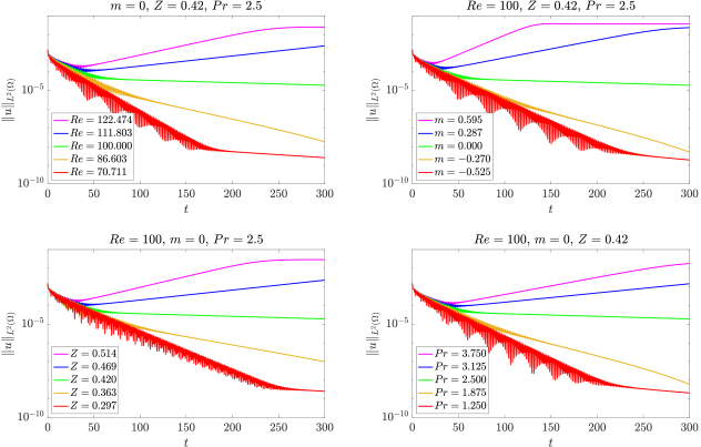
In the series of experiments below, we fix $\gamma=1.1$ and test the onset of Rayleigh-Bénard convection for several values of the four parameters Re, $m$, $Z$, Pr, for Dirichlet boundary conditions $T(x,0)=1+Z$ and $T(x,1)=1$, corresponding to the case of ideally conducting upper and lower plates. Starting with $\mathrm{Re}=100$, $m=0$, $Z=0.419524$, and $\mathrm{Pr}=2.5$, which corresponds to a flow with Rayleigh number 4000, we varied each of the four parameters individually to realize flows with Rayleigh numbers $\mathrm{Ra}\in\{2000,3000,4000,5000,6000\}$. We ran each of these simulations from time $t=0$ to time $t=300$ and plotted the evolution of the $L^{2}$-norm of the velocity field in Figure 1. In our simulations, we used a uniform triangulation of $\Omega$ with maximum element diameter $h=0.0625$, a time step $\Delta t=0.4$, penalty parameter $\eta=0.01\kappa$, and finite element spaces $V_{h}=DG_{1}(\mathcal{T}_{h})$ and $U_{h}^{\rm grad}=CG_{2}(\mathcal{T}_{h})^{2}$. One can see in Figure 1 that in each experiment, the flow begins to exhibit instability when the Rayleigh number exceeds a critical value lying somewhere between $\mathrm{Ra}=4000$ (the green curves) and $\mathrm{Ra}=5000$ (the blue curves), regardless of which of the four parameters Re, $m$, $Z$, Pr is varied.

Prescribed heat flux boundary conditions.

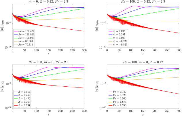
In order to illustrate the impact of the boundary condition on the critical value of the Rayleigh number, we repeat below the same experiments, now with prescribed heat flux boundary conditions $j_{q}\cdot n=q_{0}$ (nonhomogeneous Neumann boundary conditions). This boundary condition describes cases where the upper and lower plates conduct heat poorly compared with the fluid. In order to use exactly the same initial temperature profile, we set $q_{0}(x,0)=-\frac{1}{\rm Re}\frac{1}{\rm Pr}\frac{\gamma}{\gamma-1}Z$, $q_{0}(x,1)=\frac{1}{\rm Re}\frac{1}{\rm Pr}\frac{\gamma}{\gamma-1}Z$. This change of boundary condition is known to have a significant impact on the onset of convection by decreasing the critical Rayleigh number, see [30, 10] for the Boussinesq case. Figure 2 confirms this; one can see in Figure 2 that the flow begins to exhibit instability when the Rayleigh number exceeds a critical value lying somewhere between $\mathrm{Ra}=2000$ (the red curves) and $\mathrm{Ra}=3000$ (the yellow curves), regardless of which of the four parameters Re, $m$, $Z$, Pr is varied.

Refer to caption
Refer to caption
Figure 3: Left: Temperature contours during a simulation of Rayleigh-Bénard convection with $\mathrm{Re}=100$, $m=0$, $Z=2$, and $\mathrm{Pr}=2.5$, so that $\mathrm{Ra}=90909.1$. Right: Evolution of mass and energy during the simulation. The absolute deviations $|F(t)-F(0)|$ are plotted for each conserved quantity $F(t)$.

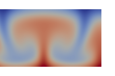
We also repeated the above experiment with $\mathrm{Re}=100$, $m=0$, $Z=2$, and $\mathrm{Pr}=2.5$, which corresponds to a much higher Rayleigh number $\mathrm{Ra}=90909.1$. We used a finer mesh with $h=0.03125$. A plot of the computed temperature at time $t\approx 14.5$ is shown in Figure 3. Note that since the prescribed heat flux $q_{0}$ satisfies $\int_{z=0}q_{0}\,{\rm d}a+\int_{z=1}q_{0}\,{\rm d}a=0$, this system conserves energy (and mass) exactly in the continuous setting. The rightmost plot in Figure 3 shows that energy and mass are conserved to machine precision in the discrete setting as well.

Appendix A Finite dimensional guiding examples

The treatment of finite dimensional systems is useful for understanding several aspects of the variational formulation for the heat conducting viscous fluid, such as the occurrence of two entropy variables ($S$ and $\Sigma$ in the Lagrangian description, $s$ and $\varsigma$ in the Eulerian description) and the form of the constraints, especially in the case when the system is not adiabatically closed, which arises when the temperature is prescribed at the boundary. We follow the variational setting developed in [25] and [28] for adiabatically closed and for open systems.

Consider a thermodynamic system described by a mechanical variable $q\in Q$ in a finite dimensional configuration manifold and an entropy variable $S\in\mathbb{R}$. We assume the system has a Lagrangian $L:TQ\times\mathbb{R}\rightarrow\mathbb{R}$ and involves a friction force $F^{\rm fr}:TQ\times\mathbb{R}\rightarrow T^{*}Q$, with $F^{\rm fr}(q,v,S)\in T^{*}_{q}Q$. The total energy and the temperature of the system are defined from $L$ by

$$E=\left\langle\frac{\partial L}{\partial\dot{q}},\dot{q}\right\rangle-L\quad\text{and}\quad T=-\frac{\partial L}{\partial S}.$$ (75)

It is assumed that the Lagrangian is such that $T>0$ for all $(q,v,S)$.

Adiabatically closed system.

When the system does not interact with its surroundings, the variational formulation is given as follows: find the curves $q(t)\in Q$, $S(t)\in\mathbb{R}$ which are critical for the variational condition

$$\delta\int_{t_{0}}^{t_{1}}L(q,\dot{q},S){\rm d}t=0,$$ (76)

subject to the phenomenological constraint

$$\frac{\partial L}{\partial S}\dot{S}=\big{\langle}F^{\rm fr},\dot{q}\big{\rangle},$$ (77)

and for variations subject to the variational constraint

$$\frac{\partial L}{\partial S}\delta S=\big{\langle}F^{\rm fr},\delta q\big{\rangle},$$ (78)

with $\delta q(t_{0})=\delta q(t_{1})=0$.

A direct application of (76)–(78) yields the coupled mechanical-thermal evolution equations:

$$\frac{d}{dt}\frac{\partial L}{\partial\dot{q}}-\frac{\partial L}{\partial q}=F^{\rm fr},\qquad\frac{\partial L}{\partial S}\dot{S}=\big{\langle}F^{\rm fr},\dot{q}\big{\rangle}.$$ (79)

With these equations, one directly gets the balance of total energy, see (75), and entropy

$$\dot{E}=0\qquad\text{and}\qquad\dot{S}=-\frac{1}{T}\big{\langle}F^{\rm fr},\dot{q}\big{\rangle}.$$ (80)

In particular, the second law requires that the force $F^{\rm fr}$ must be dissipative.

A time discretization of this variational approach has been proposed in [27, 11].

System with a heat source.

Assume that the system has an external heat source of temperature $T_{H}$ with an entropy flow $\mathcal{J}_{S,H}$. The variational formulation needs the introduction of two additional variables, namely, (i) the thermal displacement $\Gamma$ with $\dot{\Gamma}=T$ the temperature and (ii) the entropy variable $\Sigma$ with $\dot{\Sigma}=I\geq 0$ the rate of internal entropy production. The two relations $\dot{\Gamma}=T$ and $\dot{\Sigma}=I$ are not imposed a priori but follow from the variational formulation. For such systems the variational formulation is given as follows: find the curves $q(t)\in Q$, $S(t),\Gamma(t),\Sigma(t)\in\mathbb{R}$ which are critical for the variational condition

$$\delta\int_{t_{0}}^{t_{1}}\!\!\Big{[}L(q,\dot{q},S)+\dot{\Gamma}(S-\Sigma)\Big{]}{\rm d}t=0,$$ (81)

subject to the kinematic constraint

$$\frac{\partial L}{\partial S}\dot{\Sigma}=\big{\langle}F^{\rm fr},\dot{q}\big{\rangle}+\mathcal{J}_{S,H}(\dot{\Gamma}-T_{H})$$ (82)

and for variations subject to the variational constraint

$$\frac{\partial L}{\partial S}\delta\Sigma=\big{\langle}F^{\rm fr},\delta q\big{\rangle}+\mathcal{J}_{S,H}\delta\Gamma,$$ (83)

with $\delta q|_{t=t_{0},t_{1}}=0$.

Application of (81)–(83) yields the conditions

$$\delta q:\;\;\frac{d}{dt}\frac{\partial L}{\partial\dot{q}}-\frac{\partial L}{\partial q}=F^{\rm fr},\qquad\delta S:\;\;\dot{\Gamma}=-\frac{\partial L}{\partial S},\qquad\delta\Gamma:\;\;\dot{S}=\dot{\Sigma}+\mathcal{J}_{S,H}.$$

The second condition imposes that $\Gamma$ is the thermal displacement while the third condition splits the rate of entropy production $\dot{S}$ as the sum of the rate of internal entropy production $\dot{\Sigma}$ and the entropy flow rate $\mathcal{J}_{S,H}$. Finally, one gets the coupled mechanical-thermal evolution equations:

$$\frac{d}{dt}\frac{\partial L}{\partial\dot{q}}-\frac{\partial L}{\partial q}=F^{\rm fr},\qquad\frac{\partial L}{\partial S}(\dot{S}-\mathcal{J}_{S,H})=\big{\langle}F^{\rm fr},\dot{q}\big{\rangle}+\mathcal{J}_{S,H}\Big{(}-\frac{\partial L}{\partial S}-T_{H}\Big{)}.$$ (84)

With this system, the balance of energy and entropy (80) is modified as

$$\dot{E}=T_{H}\mathcal{J}_{S,H}\qquad\text{and}\qquad\dot{S}=-\frac{1}{T}\big{\langle}F^{\rm fr},\dot{q}\big{\rangle}-\frac{1}{T}\mathcal{J}_{S,H}(T-T_{H})+\mathcal{J}_{S,H}.$$ (85)

The second law requires that $-\frac{1}{T}\big{\langle}F^{\rm fr},\dot{q}\big{\rangle}\geq 0$ and $-\frac{1}{T}\mathcal{J}_{S,H}(T-T_{H})\geq 0$, while the entropy flow $\mathcal{J}_{S,H}$ can have an arbitrary sign.

Structure of the variational formulation.

In the adiabatically closed case, one passes from the phenomenological constraint (77) to the variational constraint (78) by formally replacing the time rate of changes (here $\dot{S}$ and $\dot{q}$) by $\delta$-variations (here $\delta S$ and $\delta q$). This is a general variational setting for adiabatically closed systems, see [25], which is reminiscent of the Lagrange-d’Alembert principle used in nonholonomic mechanics. The same approach is used to pass from the phenomenological constraint (4) to the variational constraint (5) for fluids in the adiabatically closed case.

In the case with a heat source the kinematic constraint is affine in the rate of changes, hence one passes from (82) to (83) by formally replacing the rate of changes (here $\dot{S}$, $\dot{q}$, and $\dot{\Gamma}$) by $\delta$-variations (here $\delta S$, $\delta q$, and $\delta\Gamma$) and by removing the affine terms associated to the exterior (here $\mathcal{J}_{S,H}T_{H}$). This is a general approach for open systems, see [28]. It is used to pass from the constraint (20) to the constraint (21) for fluids with prescribed boundary temperature

Appendix B Variational derivation of heat conducting viscous fluid equations

B.1 Lagrangian description

In the Lagrangian description, the computation of the critical condition is much simpler than its Eulerian counterpart and follows closely its finite dimensional analogue mentioned above.

For the adiabatically closed case, one gets from (3)–(5) the fluid conducting viscous fluid equation in Lagrangian form as

$$\left\{\begin{array}[]{l}\vspace{0.2cm}\displaystyle\frac{d}{dt}\frac{\delta L}{\delta\dot{\varphi}}-\frac{\delta L}{\delta\varphi}=\operatorname{DIV}P\\ \vspace{0.2cm}\displaystyle-\frac{\delta L}{\delta S}(\dot{S}+\operatorname{DIV}J_{S})=P:\nabla\dot{\varphi}+J_{S}\cdot\nabla\frac{\delta L}{\delta S},\end{array}\right.$$ (86)

together with the conditions

$$\dot{\Gamma}=-\frac{\delta L}{\delta S},\qquad\dot{\Sigma}=\dot{S}+\operatorname{DIV}J_{S}\qquad\text{and}\qquad J_{S}\cdot n=0\;\;\text{on}\;\;\partial\Omega$$ (87)

associated to the variations $\delta S$ and $\delta\Gamma$. Since $-\delta L/\delta S>0$ is identified with the temperature, the first condition implies that $\Gamma$ is the thermal displacement. The expression $\dot{S}+\operatorname{DIV}J_{S}$ is the rate of internal entropy production, positive by the second law, hence the second condition implies that $\Sigma$ is the internal entropy density. The last condition is the insulated boundary condition. It follows from the variation $\delta\Gamma$ on the boundary $\partial\Omega$ and implies that the fluid system is adiabatically closed.

For the case with prescribed boundary temperature, one applies the variational principle (3)-(20)-(21) and directly gets the equations (86) and (87) with the last equation of (87) replaced by the boundary condition

$$(J_{s}\cdot n)(\mathfrak{T}-\mathfrak{T}_{0})=0\quad\text{on}\quad\partial\Omega.$$

Here $\mathfrak{T}=-\delta L/\delta S$ is the temperature in the Lagrangian frame.

B.2 Neumann boundary conditions

We show that the variational formulation (9)–(12) yields the equations (14) together with the conditions (15).

Taking the variations in (9) and using $\delta\gamma|_{t=t_{0},t_{1}}=0$ and $u|_{\partial\Omega}=0$, we get

$$\int_{0}^{T}\int_{\Omega}\Big{[}\frac{\delta\ell}{\delta u}\cdot\delta u+\frac{\delta\ell}{\delta\rho}\delta\rho+\frac{\delta\ell}{\delta s}\delta s+\delta sD_{t}\gamma-\delta\varsigma D_{t}\gamma-\bar{D}_{t}(s-\varsigma)\delta\gamma+(s-\varsigma)\nabla\gamma\cdot\delta u\Big{]}{\rm d}x{\rm d}t=0.$$ (88)

Since $\delta s$ is arbitrary, we get the condition

$$D_{t}\gamma=-\frac{\delta\ell}{\delta s}$$ (89)

thereby recovering the first condition in (15). Making use of this condition and of the variational constraint (11) yields

$\displaystyle\int_{0}^{T}\int_{\Omega}\Big{[}\frac{\delta\ell}{\delta u}\cdot\delta u+\frac{\delta\ell}{\delta\rho}\delta\rho-\sigma:\nabla v+j_{s}\cdot\nabla(\delta\gamma+v\cdot\nabla\gamma)-\operatorname{div}(\varsigma v)\frac{\delta\ell}{\delta s}$ (90)
$\displaystyle\hskip 85.35826pt-\bar{D}_{t}(s-\varsigma)\delta\gamma+(s-\varsigma)\nabla\gamma\cdot\delta u\Big{]}{\rm d}x{\rm d}t=0.$

Since $\delta\gamma$ is arbitrary, we get

$$\bar{D}_{t}\varsigma=\bar{D}_{t}s+\operatorname{div}j_{s}\qquad\text{and}\qquad j_{s}\cdot n=0\;\;\text{on}\;\;\partial\Omega$$ (91)

thereby recovering the second and third conditions in (15). Having found these conditions, we now use $v|_{\partial\Omega}=0$ and the second condition of (12), i.e. $\delta\rho=-\operatorname{div}(\rho v)$, to rewrite (90) in the form

$$\int_{t_{0}}^{t_{1}}\int_{\Omega}\Big{[}\Big{(}\frac{\delta\ell}{\delta u}+(s-\varsigma)\nabla\gamma\Big{)}\cdot\delta u+\Big{(}\rho\nabla\frac{\delta\ell}{\delta\rho}+\varsigma\nabla\frac{\delta\ell}{\delta s}+\operatorname{div}\sigma\Big{)}\cdot v-(\operatorname{div}j_{s})v\cdot\nabla\gamma\Big{]}{\rm d}x{\rm d}t=0.$$

Using the first condition of (12), i.e. $\delta u=\partial_{t}v+[u,v]$, integrating by parts, and using the identity

$$\left(\partial_{t}+\pounds_{u}\right)\big{(}(s-\varsigma)\nabla\gamma\big{)}=\bar{D}_{t}(s-\varsigma)\nabla\gamma+(s-\varsigma)\nabla D_{t}\gamma=-\operatorname{div}j_{s}\nabla\gamma-(s-\varsigma)\nabla\frac{\delta\ell}{\delta s},$$

with $\pounds_{u}$ the Lie derivative of one-form densities, we get the first equation in (14). The second equation in (14) follows from the phenomenological constraint (10) together with (89) and the first condition in (91).

B.3 Dirichlet boundary conditions

We briefly explain how the variational formulation (9)-(22)-(23)-(12) yields the equations (14) together with the conditions in (15), with the last one replaced by (24).

We proceed similarly as in §B.2 before. Making use of (23) instead of (11) we get only the first condition in (91), namely

$$\bar{D}_{t}\varsigma=\bar{D}_{t}s+\operatorname{div}j_{s}$$ (92)

since the boundary term involving $j_{s}\cdot n$ is cancelled by the additional term in the constraint (23). The first equation in (14) follows exactly as before. Now the kinematic constraint (22), together with (89) and the first condition in (91) give both the second equation in (14) and the boundary condition (24).

B.4 Weak forms

As explained in §2.3, the constraints (10)–(11) and (22)–(23) can be written in a unified way by using the expressions $d(\cdot,\cdot,\cdot)$ and $e(\cdot,\cdot)$, see (30)–(31). The computations reviewed above can be equivalently formulated with these expressions. However, it is useful to explain how the form of the entropy equation (the second equation in (32)) emerges since its form plays a crucial role in our approach.

After taking the variation as earlier in (88), one uses in it the variational constraint with $w=1$, i.e.

$$\Big{\langle}1,\frac{\delta\ell}{\delta s}\bar{D}_{\delta}\varsigma\Big{\rangle}=-c(1,u,v)+d\Big{(}1,-\frac{\delta\ell}{\delta s},D_{\delta}\gamma\Big{)}.$$

Proceeding as earlier, this yields

$$\left\langle\bar{D}_{t}(\varsigma-s),\delta\gamma\right\rangle=-d\Big{(}1,-\frac{\delta\ell}{\delta s},\delta\gamma\Big{)},\;\;\forall\,\delta\gamma$$ (93)

which is the weak form of both (91) and (92) depending on the boundary conditions considered. One finally gets the first equation in (32), while the second equation in (32) follows from the kinematic constraint (30) in which (93) is used with $\delta\gamma=w\frac{\delta\ell}{\delta s}$. This explains the very specific forms of the two terms involving $d(\cdot,\cdot,\cdot)$ in the weak form of the entropy equation, namely

$$d\Big{(}1,-\frac{\delta\ell}{\delta s},\frac{\delta\ell}{\delta s}w\Big{)}\quad\text{and}\quad d\Big{(}w,-\frac{\delta\ell}{\delta s},\frac{\delta\ell}{\delta s}\Big{)}.$$

References

  • [1] Alboussière, T. and Y. Ricard [2017], Rayleigh-Bénard stability and the validity of quasi-Boussinesq or quasi-anelastic liquid approximations, Journal of Fluid Mechanics, 817, 264–305.
  • [2] Arnold, V. I. [1966], Sur la géométrie différentielle des des groupes de Lie de dimension infinie et ses applications à l’hydrodynamique des fluides parfaits, Ann. Inst. Fourier, Grenoble 16, 319–361.
  • [3] Arnold, D. N. [1982]. An interior penalty finite element method with discontinuous elements, SIAM Journal on Numerical Analysis, 19(4), 1749–1779.
  • [4] Arnold, D. N., F. Brezzi, B. Cockburn, and L. D. Marini [2002]. Unified analysis of discontinuous Galerkin methods for elliptic problems, SIAM Journal on Numerical Analysis, 39(5), 1749–1779.
  • [5] Bauer, W., and F. Gay-Balmaz [2019], Towards a variational discretization of compressible fluids: the rotating shallow water equations, Journal of Computational Dynamics, 6(1), 1–37
  • [6] Bormann, A. [2001], The onset of convection in the Rayleigh-Bénard problem for compressible fluids, Continuum Mech. Thermodyn., 13, 9–23, 2001.
  • [7] Brenner, S. C. and L. R. Scott [2008], The Mathematical Theory of Finite Element Methods, Third Edition, Texts in Applied Mathematics, Springer.
  • [8] F. Brezzi, L.D. Marini, and E. Süli [2004], Discontinuous Galerkin methods for first-order hyperbolic problems, Mathematical Models and Methods in Applied Sciences 14(12), 1893–1903.
  • [9] Chandrasekhar, S. [1961], Hydrodynamic and Hydromagnetic Stability, Clarendon Press: Oxford University Press.
  • [10] Chapman, C. J. and M. R. E. Proctor [1980], Nonlinear Rayleigh-Bénard convection between poorly conducting boundaries, J. Fluid Mech. 101, 759–782.
  • [11] Couéraud, B. and F. Gay-Balmaz [2020], Variational discretization of simple thermodynamical systems on Lie groups, Disc. Cont. Dyn. Syst. Ser. S13(4), 1075–1102.
  • [12] Couéraud, B. and F. Gay-Balmaz [2022], Variational discretization of the Navier-Stokes-Fourier system, arXiv:2202.03502
  • [13] Demoures, F. and F. Gay-Balmaz [2022], Unified discrete multisymplectic Lagrangian formulation for hyperelastic solids and barotropic fluids, J. Nonlin. Sc., accepted.
  • [14] Demoures, F., F. Gay-Balmaz and T. S. Ratiu [2016], Multisymplectic variational integrators for nonsmooth Lagrangian continuum mechanics, Forum Math. Sigma, 4, e19, 54p.
  • [15] Desbrun, M., E. Gawlik, F. Gay-Balmaz and V. Zeitlin [2014], Variational discretization for rotating stratified fluids, Disc. Cont. Dyn. Syst. Series A, 34, 479–511.
  • [16] Eldred, C. and F. Gay-Balmaz [2021], Thermodynamically consistent semi-compressible fluids: a variational perspective, Journal of Physics A: Mathematical and Theoretical, 54, 345701.
  • [17] Ern, A. and J.-L. Guermond [2004], Theory and Practice of Finite Elements, Applied Mathematical Sciences, 159, Springer.
  • [18] Gawlik, E. S., P. Mullen, D. Pavlov, J. E. Marsden and M. Desbrun [2011], Geometric, variational discretization of continuum theories, Physica D, 240, 1724–1760.
  • [19] Gawlik, E. S. and F. Gay-Balmaz [2020], A conservative finite element method for the incompressible Euler equations with variable density, Journal of Computational Physics 412, 109439.
  • [20] Gawlik, E. S. and F. Gay-Balmaz [2021], A variational finite element discretization of compressible flow, Found. Comput. Math., 21, 961–1001.
  • [21] Gawlik, E. S. and F. Gay-Balmaz [2021], A structure-preserving finite element method for compressible ideal and resistive MHD, Journal of Plasma Physics 87(5), 835870501.
  • [22] Gawlik, E. S. and F. Gay-Balmaz [2022], A finite element method for MHD that preserves energy, cross-helicity, magnetic helicity, incompressibility, and $\operatorname{div}B=0$, Journal of Computational Physics 450, 110847.
  • [23] Gay-Balmaz, F. [2019], A variational derivation of the nonequilibrium thermodynamics of a moist atmosphere with rain process and its pseudoincompressible approximation, Geophysical & Astrophysical Fluid Dynamics, 113:5-6, 428–465.
  • [24] Gay-Balmaz, F. and V. Putkaradze [2022], Variational geometric approach to the thermodynamics of porous media, Zeitschrift für Angewandte Mathematik und Mechanik, accepted.
  • [25] Gay-Balmaz, F. and H. Yoshimura [2017a], A Lagrangian variational formalism for nonequilibrium thermodynamics. Part I: discrete systems, J. Geom. Phys., 111, 169–193.
  • [26] Gay-Balmaz, F. and H. Yoshimura [2017b], A Lagrangian variational formalism for nonequilibrium thermodynamics. Part II: continuum systems, J. Geom. Phys., 111, 194–212.
  • [27] Gay-Balmaz, F. and H. Yoshimura [2018a], Variational discretization for the nonequilibrium thermodynamics of simple systems, Nonlinearity, 31, 1673.
  • [28] Gay-Balmaz, F. and H. Yoshimura [2018b], A variational formulation of nonequilibrium thermodynamics for discrete open systems with mass and heat transfer, Entropy, 20(3), 163.
  • [29] Gay-Balmaz, F. and H. Yoshimura [2019], From Lagrangian mechanics to nonequilibrium thermodynamics: a variational perspective, Entropy, 21(1), 8.
  • [30] Hurle, D., E. Jakeman, and E. Pike [1967], On the solution of the Bénard problem with boundaries of finite conductivity, Proc. R. Soc. Lond. A, 296, 469–475.
  • [31] Lew A., J. E. Marsden, M. Ortiz, and M. West [2003], Asynchronous variational integrators, Arch. Rational Mech. Anal., 167(2), 85–146.
  • [32] Marsden, J.E., G. W. Patrick, and S. Shkoller [1998], Multisymplectic geometry, variational integrators and nonlinear PDEs, Comm. Math. Phys., 199, 351–395.
  • [33] Marsden, J. E. and T. J. R. Hughes [1994], Mathematical foundations of elasticity, Courier Corporation.
  • [34] Marsden, J. E. and M. West [2001], Discrete mechanics and variational integrators, Acta Numer. 10, 357–514.
  • [35] Natale A. and C. Cotter [2018], A variational H(div) finite-element discretization approach for perfect incompressible fluids, IMA Journal of Numerical Analysis, 38(2), 1084.
  • [36] Pavlov, D., P. Mullen, Y. Tong, E. Kanso, J. E. Marsden, and M. Desbrun [2010], Structure-preserving discretization of incompressible fluids, Physica D, 240, 443–458.
  • [37] Robinson, F. and K. Chan [2004], Non-Boussinesq simulations of Rayleigh-Bénard convection in a perfect gas, Phys. Fluids, 16(5), 1321–1333.