Learning with Noisy Labels over Imbalanced Subpopulations

Abstract

Learning with Noisy Labels (LNL) has attracted significant attention from the research community. Many recent LNL methods rely on the assumption that clean samples tend to have “small loss”. However, this assumption always fails to generalize to some real-world cases with imbalanced subpopulations, i.e., training subpopulations varying in sample size or recognition difficulty. Therefore, recent LNL methods face the risk of misclassifying those “informative” samples (e.g., hard samples or samples in the tail subpopulations) into noisy samples, leading to poor generalization performance.

To address the above issue, we propose a novel LNL method to simultaneously deal with noisy labels and imbalanced subpopulations. It first leverages sample correlation to estimate samples’ clean probabilities for label correction and then utilizes corrected labels for Distributionally Robust Optimization (DRO) to further improve the robustness. Specifically, in contrast to previous works using classification loss as the selection criterion, we introduce a feature-based metric that takes the sample correlation into account for estimating samples’ clean probabilities. Then, we refurbish the noisy labels using the estimated clean probabilities and the pseudo-labels from the model’s predictions. With refurbished labels, we use DRO to train the model to be robust to subpopulation imbalance. Extensive experiments on a wide range of benchmarks demonstrate that our technique can consistently improve current state-of-the-art robust learning paradigms against noisy labels, especially when encountering imbalanced subpopulations.

1 Introduction

Deep Neural Networks (DNNs) have achieved remarkable progress in various domains, including computer vision [19], health care [27], natural language processing [36], etc. In practice, training datasets may contain non-negligible label noise caused by human annotators’ errors. Therefore, training against noisy labels becomes a critical problem in real-world DNN deployment and has attracted significant attention from the research communities [39, 3, 1]. In recent years, numerous works aim to develop robust learning paradigms to combat label noise [16, 11, 20]. Among those, estimated clean probabilities are critical for robust training. For example, Bootstrapping [30] assigns smaller weights to the loss of possible noisy samples. Co-teaching [11] maintains two DNN models, wherein one model is only trained by clean samples selected by another. Many State-Of-The-Art (SOTA) methods estimate the clean probabilities based on the assumption that correctly labeled samples tend to have “small loss”. For example, Dividemix [20] assumes the loss of clean and noisy samples following two Gaussian distributions, while the clean distribution has a smaller mean than the noisy one. Therefore, it utilizes a two-component Gaussian Mixture Model (GMM) to model and separate clean and noisy samples.

Figure 1: A demonstration of the learning with noisy labels over imbalanced subpopulations setup. In the Canidae-Felidae classification problem, the head subpopulations include dog and cat. The tail subpopulations include wolf and tiger. There also exist mislabeled samples, e.g., cats mislabeled as Canidae or dogs mislabeled as Felidae. The size of the images indicates the sample size of the corresponding subpopulation.

Although models trained with these methods can achieve high average performance on the overall population, they may underperform drastically in some subpopulations. The situation could become worse when the training dataset consists of “imbalanced” subpopulations. Here, “imbalanced” means training subpopulations vary in sample size or recognition difficulty. Taking a Canidae-Felidae binary classification problem as an example: the target task is to classify images into two classes, namely Canidae and Felidae, where each class consists of different subpopulations. As shown in Fig. 1, there are two subpopulations in each class (the size of the images indicates the sample size of the corresponding subpopulation). There are also some noisy samples that adversely affect the training process. In such a problem, DNNs can easily overfit on samples in the head subpopulation (e.g., dogs) while the tail samples (e.g., wolfs) and the noisy samples (e.g., cats mislabeled into “Canidae” class) tend to have large classification loss. Therefore, previous LNL methods would face the risk of misclassifying tail subpopulations into noisy samples, aggravating the damage of subpopulation imbalance. We further perform empirical studies on the corrupted Waterbird dataset to quantitatively demonstrate our point. Specifically, the representative LNL method (green bar), similar to the ERM baseline (dotted black line), performs much worse on tail subpopulations, as shown in Fig. 2(a). We suggest the cause is its bad noise identification performance on tail subpopulations as in Fig. 2(b).

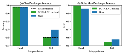
Figure 2: (a) Classification accuracy and (b) Noise identification AUC of Empirical Risk Minimization (ERM), SOTA LNL method, and our method under the problem of noisy labels over imbalanced subpopulations. The dataset is the corrupted Waterbirds dataset under 30% noise rate. We use an improved version of DivideMix as a representative LNL method, whose details are introduced in Sec. 4.

This paper studies an underexplored novel problem, i.e., learning with noisy labels over imbalanced subpopulations. As shown by the above discussions and observations, using the classification loss (e.g., cross-entropy) is inadequate to discriminate between the tail and noisy samples in this problem. Therefore, we resort to another way to estimate the label confidence (i.e., the probability of a label being clean) by considering the sample relationship in feature space. To this end, we introduce a label confidence estimation criterion named Local Label Consistency (LLC). Specifically, the LLC of one given sample is obtained by counting the number of samples in the feature-space nearest neighborhood whose labels are consistent with the given sample. The design idea behind the LLC metric is that samples from the same class typically come with high feature similarity. Utilizing this idea, we employ Gaussian Mixture Models (GMM) for clustering and mapping LLC scores to label confidence. Next, the label refurbishment framework uses label confidence as a weight to correct the given noisy label. We further integrate the refurbished labels into Distributionally Robust Optimization (DRO) [32, 44, 46], i.e., constructing the worst-case loss based on estimated label confidence. Empirically, we find the proposed refurbish-DRO paradigm can achieve better tail performance.

Through extensive experiments on corrupted Waterbird and CelebA datasets, where subpopulation imbalance and label noise coexist, we show the proposed method consistently improves the performance on tail subpopulations in contrast to current SOTA methods. As Fig. 2 shows, due to the introduction of LLC-based label confidence estimation and refurbish-DRO paradigm, our method (blue bar) achieves better classification performance and noise identification performance than previous methods (green bar) (details are in Sec. 4). Furthermore, our method also improves current state-of-the-art robust training paradigms on standard LNL benchmarks with possible implicit subpopulation imbalance, including CIFAR, Mini-WebVision, and ANIMAL-10N.

Our main contributions are summarized as follows:

• We introduce a novel problem, i.e., learning with noisy labels over imbalanced subpopulations, which has been less explored in the community. Moreover, through empirical studies, we demonstrate how previous LNL methods underperform in this new problem.

• We propose a general framework for this problem. The basic idea of the framework lies in a simple yet effective strategy that estimates label confidence based on sample relations. The label confidence is then put into our proposed refurbish-DRO paradigm to further improve robustness.

• To verify the effectiveness of our method, we conduct extensive experiments on various datasets, including corrupted datasets with imbalanced subpopulations and noisy labels (Waterbirds and CelebA) and standard LNL benchmark datasets (CIFAR, Mini-WebVision, and ANIMAL-10N). We observe that the proposed method consistently outperforms previous methods.

2 Related works

2.1 Classification-loss-based LNL methods

Deep models’ memorization effect [3] motivated the usage of the “small-loss” criterion, which has greatly improved the accuracy of LNL methods. Lots of them [16, 11, 42] filter possible noisy samples according to the agreement between the model’s predictions and given labels. For example, DivideMix [20] fits a two-component GMM in every epoch to cluster clean and noisy samples. Then it utilizes noisy samples by including them for semi-supervised learning. Similarly, SELFIE [35] and RoCL [47] obtain label confidence from cross-entropy-based criterion before using it to correct the noisy labels. However, we have observed that the classification-loss-based LNL methods obtain sub-optimal performance when training samples form imbalanced subpopulations due to their bad noise identification performance in Sec. 1.

2.2 Feature-based LNL methods

Another type of LNL method is built on the assumption that samples in the same class cluster in the feature space. These works are introduced as follows:

Sample selection Sample selection methods utilize extracted features for the calculation of sample selection criterion, e.g., either directly through the local consistency [29], largest connected component on top of a constructed graph [38, 37], or principal components from eigendecomposition [17]. However, dropping possible noisy samples leads to the loss of useful information [20], especially when the subpopulation imbalance exists. Our work instead focuses on label confidence estimation for label refurbishment, which better leverages label confidence in a more fine-grained fashion. What’s more, our method retains all samples, including those in tail subpopulations, for training.

Label refurbishment Some label refurbishment methods utilize feature representations to generate new training targets. D2L [26] adopts a label refurbishment framework and obtains optimal label confidence via back-propagating the local intrinsic dimensionality [13]. Multi-Objective Interpolation Training [29] replaces the unreliable labels (i.e., those with little same-class neighbors) with the model’s predictions. NGC [38] constructs a graph and performs label propagation to obtain pseudo-labels. On top of this framework, we are motivated to address the new setting where noisy labels and imbalanced subpopulations coexist. The refurbish-DRO strategy is proposed to encourage models to focus on worst-case performance.

Regularization Iscen et al. [15] proposed an LNL method to directly enforce local consistency using an extra loss term. Other methods, such as Sup-CL [22], and NGC [38], take advantage of contrastive learning. Sup-CL selects confident pairs for supervised contrastive learning. NGC [38] adds an extra loss term to pull samples in each class’s largest connected component together based on a constructed graph. This paper does not include these regularization strategies for simplicity and generality. However, our method is orthogonal to these regularization methods, which can be combined with our method to probably further improve performance.

2.3 Subpopulation shift

Subpopulation shift exists in many real-world data. For example, in speech recognition, the collected speech is mainly from native speakers. However, users of the speech recognition system could consist of many non-native speakers, for which the model would yield suboptimal performance [12]. Additionally, after suffering from a bad user experience, minority users are likely to stop using the product. Model retrained on future user data in turn bias toward the majority subpopulation, causing the disparity amplification problem [12].

With group information available, some methods mainly use DRO to deal with subpopulation shift [32, 44, 46, 40]. Some recent works study the domain-oblivious setting, where subpopulation memberships (i.e., subpopulation-level labels) are unknown during training. [24, 28] perform multi-round training. A preparatory model is normally trained, whose misclassified samples are up-weighted for the model’s training in the next round. On top of this, [45] uses contrastive loss to explicitly encourage the model to learn consistent representation for subpopulations in the second round. EIIL [7] uses an ERM-trained model to estimate subpopulation, followed by invariant learning [2]. However, these methods assume that label information is perfect, which could be unrealistic in practice. Our work considers a more practical problem setting, i.e., label noise and subpopulation imbalance coexist.

2.4 Other similar problem settings

A line of very recent LNL works considers some other realistic settings. NGC [38] studies the open-world noisy data. On top of handling the noisy labels, it attempts to detect out-of-distribution samples simultaneously. Different from this, our setting aims to utilize all in-distribution samples, whether mislabeled or in tail subpopulations, for training instead of excluding out-of-distribution data. H2E [41] proposes the noisy long-tailed classification problem. Our work instead focuses on a more general case, i.e., classes consist of subpopulations with different sizes or learning difficulties. Besides, our setting assumes the group annotations are unknown (instead of known class imbalance).

3 Method

3.1 Problem statement

Different from the standard supervised learning, only a noisy training dataset $\mathcal{\tilde{D}}=\{\boldsymbol{x}_{i},\tilde{\boldsymbol{y}}_{i}\}_{i=1}^{N}$ is available in LNL, where $\boldsymbol{x}_{i}$ is the input feature and $\tilde{\boldsymbol{y}}_{i}\in\{0,1\}^{C}$ denote the one-hot vector of noisy label $\tilde{y}_{i}\in\{1,\ldots,C\}$. $N$ is the number of training samples, and $C$ is the number of classes. LNL is to train a robust model which can avoid the impact of noisy labels in the training data and achieve accurate predictions on the unseen clean test dataset. The model can be viewed as a composition of a feature extractor $g(\cdot)$ and a linear classifier $f(\cdot)$ working on top of the feature extractor.

In real-world practice, it is a common case that imbalanced subpopulations exist in the dataset. This paper therefore further assumes that the dataset $\mathcal{\tilde{D}}$ consists of $K$ subpopulations, i.e., $\mathcal{\tilde{D}}=\mathcal{\tilde{D}}_{0}\cup\ldots\cup\mathcal{\tilde{D}}_{K}(K\geq C)$. The size or learning difficulty varies across subpopulations, and the subpopulation memberships are unknown during training. The model is further evaluated on each subpopulation in the clean test set.

3.2 Local label consistency for label confidence estimation

After observing the failure of using classification loss for label confidence estimation when subpopulation imbalance and label noise coexist, we resort to other criteria to tackle this issue. Considering that the cluster assumption still applies to subpopulations [4, 34], we propose to utilize the positive correlation between the label confidence and local agreement in the representation space.

Local Label Consistency We design a metric termed Local Label Consistency (LLC) to replace the conventional classification loss for label confidence estimation, which can be calculated as follows. We first obtain penultimate layer features $\boldsymbol{z}_{i}=g(\boldsymbol{x}_{i})$ and calculate the pair-wise cosine similarity $sim(\boldsymbol{z}_{i},\boldsymbol{z}_{j})=\boldsymbol{z}_{i}^{\mathrm{T}}\boldsymbol{z}_{j}/||\boldsymbol{z}_{i}||\,||\boldsymbol{z}_{j}||$. The k-nearest neighbors of each node (sample) $\mathcal{N}_{k}(i)$ are selected according to the calculated pair-wise cosine similarities. Then, the LLC of $i$-th sample is calculated as the proportion of neighbors with the same class label,

$$\mathrm{LLC}_{i}=\sum_{j\in\mathcal{N}_{k}(i)}\mathds{1}[\tilde{\boldsymbol{y}}_{i}=\tilde{\boldsymbol{y}}_{j}]$$ (1)

where $\mathds{1}[\cdot]$ is the indicator function. It equals 1 if the equation in it holds. Otherwise, it equals 0.

Label confidence After obtaining the LLC scores of samples, we perform unsupervised clustering on these scores to obtain the label confidence, i.e., clean probability: $\mathrm{p}(y=\tilde{y}|\boldsymbol{x})$, where $y$ is the inaccessible ground-truth label. Specifically, in every epoch, we use the current model to obtain all samples’ LLC scores. Then, we use a one-dimensional two-component GMM to fit the distribution of these LLC scores. The corresponding parameters are estimated using the Expectation–Maximization (EM) algorithm (We elaborate on the details in the supplementary material.). After this, The probability of each sample belonging to the GMM component with a bigger mean can be obtained, which is used as the label confidence $w_{i}$ for $i$-th sample. The overall pipeline is shown in Alg. 1.

Algorithm 1 Our method

Input: Noisy dataset $\tilde{\mathcal{D}}=\{(\boldsymbol{x}_{i},\tilde{\boldsymbol{y}}_{i})\}^{N}_{i=1}$, # epochs for warm up $E_{warmup}$, # total epochs $E$, ERM training strategy $\text{Train}(\text{dateset},\text{parameters})$, robust training strategy with label confidence $\text{RobustTrain}(\text{dateset},\text{label confidence},\text{parameters})$.
Output: Model’s parameters $\theta$

1:Randomly initialize $\theta$.

2:for $e=0$ to $E_{warmup}$ do $\triangleright$ standard ERM

3:     $\text{Train}(\tilde{\mathcal{D}},\theta)$

4:end for

5:for $e=1$ to $E$ do

6:     for $i=0$ to $N$ do

7:         obtain $\mathcal{N}_{k}(i)$ based the learned representation $\boldsymbol{z}_{i}=g(\boldsymbol{x}_{i})$

8:         obtain every sample’s LLC score $\mathrm{LLC}_{i}=\sum_{j\in\mathcal{N}_{k}(i)}\mathds{1}[\tilde{\boldsymbol{y}}_{i}=\tilde{\boldsymbol{y}}_{j}]$

9:     end for

10:     fit $\mathrm{GMM}$ on $\{\mathrm{LLC}_{i}\}_{i=0}^{N}$ and obtain per-sample confidence $\mathcal{W}=\{w_{i}\}_{i=0}^{N}$

11:     Robust training for one epoch: $\theta=\text{RobustTrain}(\tilde{\mathcal{D}},\mathcal{W},\theta)$ following Alg. 2

12:end for

Algorithm 2 RobustTrain

Input: Noisy dataset $\tilde{\mathcal{D}}$, label confidence $\mathcal{W}$, batch size $B$ Output: Model’s parameters $\theta$

1:for $n=0,1,...,\frac{|\tilde{\mathcal{D}}|}{B}$ do

2:     Randomly draw a mini-batch $\{(\boldsymbol{x}_{i},\tilde{\boldsymbol{y}}_{i},w_{i})\}_{i=1}^{B}$ from $\tilde{\mathcal{D}}$ and $\mathcal{W}$

3:     for $i=0$ to $B$ do

4:         $\hat{\boldsymbol{y}}_{i}=\text{p}(\boldsymbol{y}\mid\alpha(\boldsymbol{x}_{i});\theta)$ $\triangleright$ pseudo-label

5:         $\boldsymbol{y}^{*}_{i}=w_{i}\tilde{\boldsymbol{y}}_{i}+(1-w_{i})\hat{\boldsymbol{y}}_{i}$ $\triangleright$ refurbish label

6:     end for

7:     $\mathcal{L}=\{\text{H}(\boldsymbol{y}_{i}^{*},\text{p}(\boldsymbol{y}\mid\mathcal{A}(\boldsymbol{x}_{i});\theta))\}_{i=1}^{B}$

8:     $\mathcal{L}^{\prime}=\mathop{\arg\max}\limits_{\mathcal{L}^{\prime}\subset\mathcal{L}}\sum_{\ell_{i}\in\mathcal{L}^{\prime}}\ell_{i}\quad\mathrm{s.t.}\,|\mathcal{L}^{\prime}|=|\mathcal{L}|*\tau\%$

9:     update $\theta$ according to the gradient $\nabla\frac{1}{|\mathcal{L}^{\prime}|}\sum_{\ell_{i}\in\mathcal{L}^{\prime}}\ell_{i}$

10:end for

3.3 Robust training

Refurbish-DRO We aim to utilize the estimated label confidence to improve robustness against both label noise and subpopulation imbalance. To this end, we proposed the refurbish-DRO paradigm. Specifically, we first generate refurbished labels on top of it to supervise training [30], which is a convex combination between noisy labels and pseudo-labels:

$$\hat{\boldsymbol{y}}_{i} =\text{p}(\boldsymbol{y}\mid\boldsymbol{x}_{i};\theta)$$ (2)

$$\boldsymbol{y}^{*}_{i} =w_{i}\tilde{\boldsymbol{y}}_{i}+(1-w_{i})\hat{\boldsymbol{y}}_{i}$$

where $w_{i}$ is the estimated label confidence of $i$-th sample, pseudo-label $\hat{\boldsymbol{y}}_{i}$ are from model’s predictions, and the refurbished label $\boldsymbol{y}^{*}_{i}$, replacing the original noisy label $\tilde{\boldsymbol{y}}_{i}$, acts as the corrected supervision signal, $\theta$ represents the model parameters. The refurbishment can be seen as a balance between given supervision (noisy labels) and self-supervision (pseudo-labels), where the label confidence is the weight to adaptively adjust the contribution of each component.

Then, we attempt to further ensure the model’s fairness for tail subpopulations or minority samples (i.e., robust accuracy). To solve this problem, previous studies [14, 31] seek to minimize the worst-case empirical risk,

$$\mathop{\arg\min}\limits_{\theta}\left\{\mathop{\max}\limits_{k\in{1,\ldots,K}}\frac{1}{|\mathcal{D}_{k}|}\sum_{(x_{i},y_{i})\in\mathcal{D}_{k}}\ell_{i}\right\}$$ (3)

where $\ell_{i}$ can be any surrogate loss function.

However, Eq. (3) needs group annotations and cannot cope with noisy labels. Thus, we attempt to design a robust training method that does not require group annotations and is also applicable in the coexistence of label noise. It has been found that deep models tend to fit head groups with commonly shared patterns (e.g., water background for waterbirds) instead of tail groups with infrequent patterns (e.g., land background for waterbirds) [31, 24]. Therefore, the tail subpopulations can be heuristically identified by the discrepancy between predicted probabilities and the ground-truth labels [24, 28, 43]. Those with bigger losses (between the ground-truth label) are more likely to come from more challenging groups. To approximate Eq. (3), a simple but effective modification of the original loss is adopted. Specifically, we rank the samples in every mini-batch based on the loss between the model’s predicted distribution and the refurbished label distribution and only select the top-$\tau$% for training:

$$\mathop{\arg\min}\limits_{\theta}\left\{\mathop{\max}\limits_{\mathcal{L}^{\prime}\subset\mathcal{L}}\sum_{\ell_{i}\in\mathcal{L}^{\prime}}\ell_{i}\right\}\quad\mathrm{s.t.}\,|\mathcal{L}^{\prime}|=|\mathcal{L}|*\tau\%$$ (4)

where $\ell_{i}$ is the loss of $i$-th sample, $\mathcal{L}$ is a set of loss values of samples in the current batch. We instead use the obtained refurbished label $\boldsymbol{y}^{*}_{i}$ in Eq. (2):

$$\ell_{i} =\text{H}(\boldsymbol{y}^{*}_{i},\text{p}(\boldsymbol{y}\mid\boldsymbol{x}_{i};\theta))$$ (5)

where $\mathrm{H}(\cdot)$ is the cross-entropy function. In this way, we avoid using the given noisy labels to calculate the loss and obtain the uncertainty set $\mathcal{L}^{\prime}$ [24], which would certainly fail due to noisy samples’ interference. Our final learning target, therefore, focuses more on the difficult-to-learn samples while preventing the model from potentially overfitting the head subpopulation.

Weak-strong augmentation schema To generate high-quality pseudo-labels and improve generalization, we employ the recently weak-strong data augmentation schema [33]. Specifically, The model’s predictions on the weakly augmented images $\alpha(\cdot)$ is used to generate pseudo-labels, i.e., we change the first equation in (2) to:

$$\hat{\boldsymbol{y}}_{i}=\text{p}(\boldsymbol{y}\mid\alpha(\boldsymbol{x}_{i});\theta)$$ (6)

The model’s predictions on the strongly augmented images $\mathcal{A}(\cdot)$ (e.g., applied with multiple geometric and color transformations) are enforced to be consistent with the pseudo-labels, i.e., we change the loss in equation (5) to:

$$\text{H}(\boldsymbol{y}_{i}^{*},\text{p}(\boldsymbol{y}\mid\mathcal{A}(\boldsymbol{x}_{i});\theta))$$ (7)

The weak-strong augmentation schema in our LNL method can be seen as a special variant of consistency regularization or self-training method. We set the weak augmentation $\alpha$ as a random crop followed by a random horizontal flip. For the strong augmentation $\mathcal{A}$, we use the FixMatch version of RandAugment [8]. More details are given in the supplementary material.

Co-training Following previous works [11, 20], two models with the same structure but different random initializations are simultaneously trained. We use the confidence produced by one model to guide the training of its peer, i.e., the estimated label confidence from one model is used by another model and vice versa. Furthermore, we also use the co-teaching schema as in [20], i.e., pseudo-labels are generated from the ensemble (average) predictions of two models.

4 Experiments

Dataset	CelebA
Noise rate	15%		20%		25%		30%
Method/Group	Avg.	Worst	Avg.	Worst	Avg.	Worst	Avg.	Worst
ERM	95.60	34.44	95.50	28.88	95.53	30.00	95.20	20.00
DivideMix∗	95.20	28.33	95.22	28.88	95.14	31.11	95.05	20.55
Ours	95.12	36.66	95.08	34.44	95.12	41.66	95.24	28.33
Dataset	Waterbirds
Noise rate	25%		30%		35%		40%
Method/Group	Avg.	Worst	Avg.	Worst	Avg.	Worst	Avg.	Worst
ERM	83.15	48.60	78.65	52.96	79.53	64.17	73.66	48.29
DivideMix∗	85.92	55.61	79.32	54.67	74.37	47.82	Not converged
Ours	88.40	70.56	86.09	69.31	84.93	71.88	79.77	59.97

Table 1: Comparison over the corrupted Waterbirds and CelebA dataset. ^∗We use the same label confidence estimation method as DivideMix. For a fair comparison, we replace its other components and training schemas with ours.

We conduct experiments on different settings: 1). datasets with different levels of noisy labels and explicit subpopulation size imbalance. 2). datasets with both synthetic and real-world noisy labels (standard LNL benchmarks) that inevitably exist implicit subpopulation recognition difficulty or size imbalance. All comparisons are made under the same model architecture, and the details are in the supplementary material.

4.1 Comparison on corrupted datasets with explicit imbalanced subpopulations

We evaluate our proposed method in the new setting of the coexistence of noisy labels and imbalanced subpopulation on the corrupted Waterbirds dataset [32] and corrupted CelebA dataset [25]. We use the Waterbirds dataset from [32], which has 4,795 training samples consisting of waterbird and landbird images. 95% of waterbirds are placed against water backgrounds, and the remaining 5% of waterbirds are placed against land backgrounds. Similarly, 95% of landbirds are placed against land backgrounds, and the remaining 5% of landbirds are placed against water backgrounds. Then we randomly flip the labels of 25%/30%/35%/40% of samples to obtain the corrupted dataset. CelebA’s training set includes 71,629 females with dark hair, 66,874 males with dark hair, 22,880 females with blond hair, and only 1,387 males with blond hair. The prediction task is to tell the color of the sample’s hair. Therefore, blond-haired men can be seen as the tail subpopulation, while others can be seen as head subpopulations. It’s also worth noting that the imbalance ratio of CelebA is bigger than that of Waterbirds. Therefore, we apply lighter noise corruption, i.e., labels of 15%/20%/25%/30% of samples are corrupted to form the corrupted CelebA dataset. These two datasets both have provided extra validation and test sets for hyper-parameter tuning and testing. We save the best-performed model on the validation set and report its test accuracy. To evaluate the model’s performance on the overall population and tail subpopulation, we report the average test accuracy and the accuracy of the subpopulation that the model performs worst on, respectively.

For comparison, we include two methods: 1). ERM, i.e., using no extra robustness training method to optimize the model. 2). improved DivideMix. It uses DivideMix’s label confidence estimation method but has the same training schema as ours to ensure a fair comparison. Backbone models of two baselines are also the same as our method.

In Table 1, we compare the proposed method with the improved DivideMix and the ERM model on two datasets. The ERM model learns the spurious correlations, e.g., water background and waterbirds, which leads to worse performance on some tail subpopulations (i.e., worst-case accuracy) than that on average. The improved DivideMix with the previous classification-loss-based confidence estimation also achieves low worst-case accuracy, sometimes even worse than the ERM baseline. This is because it would misclassify clean subpopulations into noise and exclude them from the training objective, aggravating the subpopulation imbalance problem. Instead, our robust training method better combats spurious correlations on the corrupted Waterbirds dataset, yielding much better generalization ability on the subpopulations (worst-case accuracy improved by 7.7%-14.95%). The model’s average accuracy on the overall population also improved by 2.5%-6.8%. We provide more results on different imbalance ratios in the supplementary material. On CelebA, our method also consistently achieves the best worst-case accuracy (improve the baselines by 2.2%-10.5%) while keeping the average accuracy greater than 95%.

We also notice that the increase in noise rate does not necessarily lead to the decrease of worst-case performance in Table 1. We speculate that uniformly distributed noise may act as a regularization that encourages the model to make more diverse predictions.

Dataset		CIFAR-10					CIFAR-100
Noise type		Sym.				Asym.	Sym.
Method/Noise ratio		20%	50%	80%	90%	40%	20%	50%	80%	90%
Co-teaching+	Best	89.5	85.7	67.4	47.9	-	65.6	51.8	27.9	13.7
	Last	88.2	84.1	45.5	30.1	-	64.1	45.3	15.5	8.8
Meta-Learning	Best	92.9	89.3	77.4	58.7	89.2	68.5	59.2	42.4	19.5
	Last	92.0	88.8	76.1	58.3	88.6	67.7	58.0	40.1	14.3
M-correction	Best	94.0	92.0	86.8	69.1	87.4	73.9	66.1	48.2	24.3
	Last	93.8	91.9	86.6	68.7	86.3	73.4	65.4	47.6	20.5
DivideMix	Best	96.1	94.6	93.2	76.0	93.4	77.3	74.6	60.2	31.5
	Last	95.7	94.4	92.9	75.4	92.1	76.9	74.2	59.6	31.0
Ours	Best	96.1	95.9	95.9	94.8	94.7	79.2	75.5	67.7	51.0
	Last	96.0	95.8	95.8	94.6	94.1	78.1	74.5	65.3	49.2

Table 2: Comparison with state-of-the-art LNL methods on corrupted CIFAR. Sym. and Asym. are symmetric and asymmetric for short, respectively. The best results are indicated in bold. Other methods’ results are from [20].

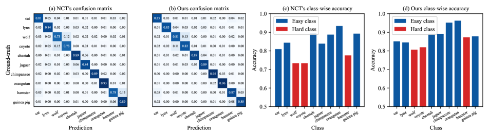
Figure 3: The confusion matrix and class-wise accuracy of previous SOTA NCT and our method on ANIMAL-10N. Other than average accuracy, our method achieves even more significant improvement in some difficult-to-learn classes. We define a class as hard when NCT’s accuracy is lower than 80%. We reproduce the results of NCT using their official GitHub code.

4.2 Comparison with state-of-the-art methods on standard LNL benchmarks

We further benchmark the proposed method on common LNL experimental settings using CIFAR [18] with different levels and types of synthetic noises, as well as the real-world noisy dataset Mini-WebVision [23] and ANIMAL-10N [35]. We use ANIMAL-10N as an example of a real-world noisy dataset with implicit subpopulation imbalance.

4.2.1 CIFAR-10, CIFAR-100 with synthetic label noise

Performance on randomly generated uniform (symmetric) noise can generally indicate the effectiveness of robust training methods. Thus, we compare our method with Co-teaching+ [42], Meta-learning [21], DivideMix [20] on uniformly corrupted CIFAR. Besides, following previous work [20], we also experiment with CIFAR-10 corrupted by a pre-defined transition matrix. The corruption mimics the real-world noise in which samples are liked to be labeled into similar classes, e.g., deer to horse. We report the performance of the last epoch and the best epoch following previous methods.

Table 2 shows that our method consistently achieves competitive performance against previous methods under various noise rates and synthetic noise types.

4.2.2 Mini-WebVision and ANIMAL-10N with real-world label noise

The label noise and distribution shift could be more complex in the wild [10]. Therefore, it is necessary to conduct experiments on real-world noisy datasets. WebVision [39] includes large-scale web images. We follow [5], using the first 50 classes. Besides, the validation set of ImageNet ILSVRC12 [9] is used. ANIMAL-10N [35] includes 10 animals, where 5 pairs of them are alike, such as cat vs. lynx and jaguar vs. cheetah.

For comparison on Mini-WebVision, results of Co-teaching [11], DivideMix [20], NGC [38] are reported. Our method outperforms previous methods by 1.56% top-1 accuracy on the test set, as shown in Table 3. The results validate the effectiveness of our approach on real-world noise.

Method	Mini-WebVision		ILSVRC12
	top-1	top-5	top-1	top-5
Co-teaching	63.58	85.20	61.48	84.70
DivideMix	77.32	91.64	75.20	90.84
NGC	79.16	91.84	74.44	91.04
Ours	80.72	93.19	76.76	93.76

Table 3: Comparison with other methods on Mini-WebVision. The results of other methods are from [20, 38].

We choose NCT [6], the previous best method on ANIMAL-10N, for the comparison in Fig. 3 (comparison with more methods is in the supplementary material). ANIMAL-10N, as a real-world class-balanced dataset, has different learning difficulties across classes. Wolf, coyote, and hamster are harder to recognize for NCT, as shown in Fig. 3 (a) and (c). The results support our argument that real-world datasets could have implicit “imbalanced” subpopulations varying in learning difficulties. Our average accuracy is 4.1% higher than NCT (88.2% vs. 84.1%), while the improvement mainly comes from the more difficult classes (i.e., those NCT performs worse on), e.g., on wolf is 80.6% vs. 73.4% and on coyote is 82.0% vs. 73.3%. Our model achieves better worst-case (in terms of class) performance, which verifies that our method successfully addresses such imbalance, improving generalization ability.

4.2.3 Ablation study

We conduct the ablation study to verify the effectiveness of the two main components, i.e., LLC and refurbish-DRO. We replace LLC with classification-loss-based label confidence estimation or remove the DRO strategy and compare the performances of these variants. The performances of four combinations are illustrated in Table 4. The proposed two components both bring remarkable improvement upon the baselines. Adding the refurbish-DRO strategy on both classification-loss-based LNL (second row vs. first row) and feature-based LNL (fourth row vs. third row) can improve worst-case performance. The combination of LLC and refurbish-DRO strategy achieves consistent best results under various noise rates.

Component/Group		25% noise rate		30% noise rate
LLC	Refurbish-DRO	Avg.	Worst	Avg.	Worst
		85.92	55.61	79.32	54.67
	✓	84.90	59.81	79.58	55.29
✓		87.63	67.60	82.14	64.39
✓	✓	88.40	70.56	86.06	69.31
Component/Group		35% noise rate		40% noise rate
LLC	Refurbish-DRO	Avg.	Worst	Avg.	Worst
		73.95	26.79	Not converged
	✓	74.54	49.22	79.39	49.06
✓		82.50	65.90	74.78	51.09
✓	✓	84.93	71.88	79.77	59.97

Table 4: Ablation study on the corrupted Waterbirds dataset.

We also conduct sensitivity tests for two hyper-parameters, i.e., nearest neighbor number $k$ in KNN for the calculation of LLC and the threshold $\tau$ for refurbish-DRO. The results are given in Fig. 4, where we found that our proposed method can generally achieve robust high performance with different choices of $k$ and $\tau$.

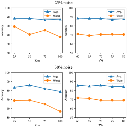
Figure 4: Hyper-parameter sensitivity tests for the nearest neighbor numbers $k$ and threshold $\tau$ for refurbish-DRO on the corrupted Waterbirds dataset under 25% and 30% noise.

5 Conclusion

This paper studies a realistic but challenging problem: learning with noisy labels over imbalanced subpopulations. Plenty of works concentrating on learning with noisy labels or distribution shifts (imbalanced subpopulations) rarely address the contradiction in the coexistence of label noise and subpopulation shifts. How to deal with those samples that are perceptually inconsistent with the learned model but could be either informative or noisy is still an open question. As a pioneer exploration, our method first resorts to label confidence estimation based on label consistency in feature space, alleviating the misidentification in conventional classification-loss-based LNL methods. Using the estimated label confidence, we propose the refurbish-DRO paradigm, making the model less susceptible to spurious correlations. Extensive experiments verify the effectiveness of our method. Our work has the potential to motivate researchers to explore more realistic problems to facilitate the robust deployment of deep models in the wild.

References

- [1] Dana Angluin and Philip D. Laird. Learning from noisy examples. Mach. Learn., 2(4):343–370, 1987.
- [2] Martín Arjovsky, Léon Bottou, Ishaan Gulrajani, and David Lopez-Paz. Invariant risk minimization. CoRR, abs/1907.02893, 2019.
- [3] Devansh Arpit, Stanisław Jastrzębski, Nicolas Ballas, David Krueger, Emmanuel Bengio, Maxinder S Kanwal, Tegan Maharaj, Asja Fischer, Aaron Courville, Yoshua Bengio, et al. A closer look at memorization in deep networks. In International Conference on Machine Learning, pages 233–242. PMLR, 2017.
- [4] Olivier Chapelle, Mingmin Chi, and Alexander Zien. A continuation method for semi-supervised svms. In William W. Cohen and Andrew W. Moore, editors, Machine Learning, Proceedings of the Twenty-Third International Conference (ICML 2006), Pittsburgh, Pennsylvania, USA, June 25-29, 2006, volume 148 of ACM International Conference Proceeding Series, pages 185–192. ACM, 2006.
- [5] Pengfei Chen, Ben Ben Liao, Guangyong Chen, and Shengyu Zhang. Understanding and utilizing deep neural networks trained with noisy labels. In International Conference on Machine Learning, pages 1062–1070. PMLR, 2019.
- [6] Yingyi Chen, Xi Shen, Shell Xu Hu, and Johan A. K. Suykens. Boosting co-teaching with compression regularization for label noise. In IEEE Conference on Computer Vision and Pattern Recognition Workshops, CVPR Workshops 2021, virtual, June 19-25, 2021, pages 2688–2692. Computer Vision Foundation / IEEE, 2021.
- [7] Elliot Creager, Jörn-Henrik Jacobsen, and Richard S. Zemel. Environment inference for invariant learning. In Marina Meila and Tong Zhang, editors, Proceedings of the 38th International Conference on Machine Learning, ICML 2021, 18-24 July 2021, Virtual Event, volume 139 of Proceedings of Machine Learning Research, pages 2189–2200. PMLR, 2021.
- [8] Ekin D Cubuk, Barret Zoph, Jonathon Shlens, and Quoc V Le. Randaugment: Practical automated data augmentation with a reduced search space. In Proceedings of the IEEE/CVF Conference on Computer Vision and Pattern Recognition Workshops, pages 702–703, 2020.
- [9] Jia Deng, Wei Dong, Richard Socher, Li-Jia Li, Kai Li, and Li Fei-Fei. Imagenet: A large-scale hierarchical image database. In 2009 IEEE conference on computer vision and pattern recognition, pages 248–255. Ieee, 2009.
- [10] Bo Han, Quanming Yao, Tongliang Liu, Gang Niu, Ivor W. Tsang, James T. Kwok, and Masashi Sugiyama. A survey of label-noise representation learning: Past, present and future. CoRR, abs/2011.04406, 2020.
- [11] Bo Han, Quanming Yao, Xingrui Yu, Gang Niu, Miao Xu, Weihua Hu, Ivor Tsang, and Masashi Sugiyama. Co-teaching: Robust training of deep neural networks with extremely noisy labels. arXiv preprint arXiv:1804.06872, 2018.
- [12] Tatsunori B. Hashimoto, Megha Srivastava, Hongseok Namkoong, and Percy Liang. Fairness without demographics in repeated loss minimization. In Jennifer G. Dy and Andreas Krause, editors, Proceedings of the 35th International Conference on Machine Learning, ICML 2018, Stockholmsmässan, Stockholm, Sweden, July 10-15, 2018, volume 80 of Proceedings of Machine Learning Research, pages 1934–1943. PMLR, 2018.
- [13] Michael E Houle. Local intrinsic dimensionality i: an extreme-value-theoretic foundation for similarity applications. In International Conference on Similarity Search and Applications, pages 64–79. Springer, 2017.
- [14] Weihua Hu, Gang Niu, Issei Sato, and Masashi Sugiyama. Does distributionally robust supervised learning give robust classifiers? In Jennifer G. Dy and Andreas Krause, editors, Proceedings of the 35th International Conference on Machine Learning, ICML 2018, Stockholmsmässan, Stockholm, Sweden, July 10-15, 2018, volume 80 of Proceedings of Machine Learning Research, pages 2034–2042. PMLR, 2018.
- [15] Ahmet Iscen, Jack Valmadre, Anurag Arnab, and Cordelia Schmid. Learning with neighbor consistency for noisy labels. CoRR, abs/2202.02200, 2022.
- [16] Lu Jiang, Zhengyuan Zhou, Thomas Leung, Li-Jia Li, and Li Fei-Fei. Mentornet: Learning data-driven curriculum for very deep neural networks on corrupted labels. In International Conference on Machine Learning, pages 2304–2313. PMLR, 2018.
- [17] Taehyeon Kim, Jongwoo Ko, Sangwook Cho, Jinhwan Choi, and Se-Young Yun. FINE samples for learning with noisy labels. In Marc’Aurelio Ranzato, Alina Beygelzimer, Yann N. Dauphin, Percy Liang, and Jennifer Wortman Vaughan, editors, Advances in Neural Information Processing Systems 34: Annual Conference on Neural Information Processing Systems 2021, NeurIPS 2021, December 6-14, 2021, virtual, pages 24137–24149, 2021.
- [18] Alex Krizhevsky, Geoffrey Hinton, et al. Learning multiple layers of features from tiny images. 2009.
- [19] Alex Krizhevsky, Ilya Sutskever, and Geoffrey E Hinton. Imagenet classification with deep convolutional neural networks. Advances in neural information processing systems, 25:1097–1105, 2012.
- [20] Junnan Li, Richard Socher, and Steven CH Hoi. Dividemix: Learning with noisy labels as semi-supervised learning. arXiv preprint arXiv:2002.07394, 2020.
- [21] Junnan Li, Yongkang Wong, Qi Zhao, and Mohan S Kankanhalli. Learning to learn from noisy labeled data. In Proceedings of the IEEE/CVF Conference on Computer Vision and Pattern Recognition, pages 5051–5059, 2019.
- [22] Shikun Li, Xiaobo Xia, Shiming Ge, and Tongliang Liu. Selective-supervised contrastive learning with noisy labels. CoRR, abs/2203.04181, 2022.
- [23] Wen Li, Limin Wang, Wei Li, Eirikur Agustsson, and Luc Van Gool. Webvision database: Visual learning and understanding from web data. arXiv preprint arXiv:1708.02862, 2017.
- [24] Evan Zheran Liu, Behzad Haghgoo, Annie S. Chen, Aditi Raghunathan, Pang Wei Koh, Shiori Sagawa, Percy Liang, and Chelsea Finn. Just train twice: Improving group robustness without training group information. In Marina Meila and Tong Zhang, editors, Proceedings of the 38th International Conference on Machine Learning, ICML 2021, 18-24 July 2021, Virtual Event, volume 139 of Proceedings of Machine Learning Research, pages 6781–6792. PMLR, 2021.
- [25] Ziwei Liu, Ping Luo, Xiaogang Wang, and Xiaoou Tang. Deep learning face attributes in the wild. In 2015 IEEE International Conference on Computer Vision, ICCV 2015, Santiago, Chile, December 7-13, 2015, pages 3730–3738. IEEE Computer Society, 2015.
- [26] Xingjun Ma, Yisen Wang, Michael E Houle, Shuo Zhou, Sarah Erfani, Shutao Xia, Sudanthi Wijewickrema, and James Bailey. Dimensionality-driven learning with noisy labels. In International Conference on Machine Learning, pages 3355–3364. PMLR, 2018.
- [27] Riccardo Miotto, Fei Wang, Shuang Wang, Xiaoqian Jiang, and Joel T Dudley. Deep learning for healthcare: review, opportunities and challenges. Briefings in Bioinformatics, 19(6):1236–1246, 05 2017.
- [28] Jun Hyun Nam, Hyuntak Cha, Sungsoo Ahn, Jaeho Lee, and Jinwoo Shin. Learning from failure: Training debiased classifier from biased classifier. CoRR, abs/2007.02561, 2020.
- [29] Diego Ortego, Eric Arazo, Paul Albert, Noel E. O’Connor, and Kevin McGuinness. Multi-objective interpolation training for robustness to label noise. In IEEE Conference on Computer Vision and Pattern Recognition, CVPR 2021, virtual, June 19-25, 2021, pages 6606–6615. Computer Vision Foundation / IEEE, 2021.
- [30] Scott Reed, Honglak Lee, Dragomir Anguelov, Christian Szegedy, Dumitru Erhan, and Andrew Rabinovich. Training deep neural networks on noisy labels with bootstrapping. arXiv preprint arXiv:1412.6596, 2014.
- [31] Shiori Sagawa, Pang Wei Koh, Tatsunori B. Hashimoto, and Percy Liang. Distributionally robust neural networks for group shifts: On the importance of regularization for worst-case generalization. CoRR, abs/1911.08731, 2019.
- [32] Shiori Sagawa, Pang Wei Koh, Tatsunori B. Hashimoto, and Percy Liang. Distributionally robust neural networks. In 8th International Conference on Learning Representations, ICLR 2020, Addis Ababa, Ethiopia, April 26-30, 2020. OpenReview.net, 2020.
- [33] Kihyuk Sohn, David Berthelot, Chun-Liang Li, Zizhao Zhang, Nicholas Carlini, Ekin D Cubuk, Alex Kurakin, Han Zhang, and Colin Raffel. Fixmatch: Simplifying semi-supervised learning with consistency and confidence. arXiv preprint arXiv:2001.07685, 2020.
- [34] Nimit Sharad Sohoni, Jared Dunnmon, Geoffrey Angus, Albert Gu, and Christopher Ré. No subclass left behind: Fine-grained robustness in coarse-grained classification problems. In Hugo Larochelle, Marc’Aurelio Ranzato, Raia Hadsell, Maria-Florina Balcan, and Hsuan-Tien Lin, editors, Advances in Neural Information Processing Systems 33: Annual Conference on Neural Information Processing Systems 2020, NeurIPS 2020, December 6-12, 2020, virtual, 2020.
- [35] Hwanjun Song, Minseok Kim, and Jae-Gil Lee. Selfie: Refurbishing unclean samples for robust deep learning. In International Conference on Machine Learning, pages 5907–5915. PMLR, 2019.
- [36] Ashish Vaswani, Noam Shazeer, Niki Parmar, Jakob Uszkoreit, Llion Jones, Aidan N. Gomez, Lukasz Kaiser, and Illia Polosukhin. Attention is all you need. In Isabelle Guyon, Ulrike von Luxburg, Samy Bengio, Hanna M. Wallach, Rob Fergus, S. V. N. Vishwanathan, and Roman Garnett, editors, Advances in Neural Information Processing Systems 30: Annual Conference on Neural Information Processing Systems 2017, December 4-9, 2017, Long Beach, CA, USA, pages 5998–6008, 2017.
- [37] Pengxiang Wu, Songzhu Zheng, Mayank Goswami, Dimitris Metaxas, and Chao Chen. A topological filter for learning with label noise. arXiv preprint arXiv:2012.04835, 2020.
- [38] Zhi-Fan Wu, Tong Wei, Jianwen Jiang, Chaojie Mao, Mingqian Tang, and Yu-Feng Li. Ngc: A unified framework for learning with open-world noisy data. In Proceedings of the IEEE/CVF International Conference on Computer Vision, pages 62–71, 2021.
- [39] Tong Xiao, Tian Xia, Yi Yang, Chang Huang, and Xiaogang Wang. Learning from massive noisy labeled data for image classification. In Proceedings of the IEEE conference on computer vision and pattern recognition, pages 2691–2699, 2015.
- [40] Huaxiu Yao, Yu Wang, Sai Li, Linjun Zhang, Weixin Liang, James Zou, and Chelsea Finn. Improving out-of-distribution robustness via selective augmentation. In Kamalika Chaudhuri, Stefanie Jegelka, Le Song, Csaba Szepesvári, Gang Niu, and Sivan Sabato, editors, International Conference on Machine Learning, ICML 2022, 17-23 July 2022, Baltimore, Maryland, USA, volume 162 of Proceedings of Machine Learning Research, pages 25407–25437. PMLR, 2022.
- [41] Xuanyu Yi, Kaihua Tang, Xian-Sheng Hua, Joo-Hwee Lim, and Hanwang Zhang. Identifying hard noise in long-tailed sample distribution. In Shai Avidan, Gabriel J. Brostow, Moustapha Cissé, Giovanni Maria Farinella, and Tal Hassner, editors, Computer Vision - ECCV 2022 - 17th European Conference, Tel Aviv, Israel, October 23-27, 2022, Proceedings, Part XXVI, volume 13686 of Lecture Notes in Computer Science, pages 739–756. Springer, 2022.
- [42] Xingrui Yu, Bo Han, Jiangchao Yao, Gang Niu, Ivor Tsang, and Masashi Sugiyama. How does disagreement help generalization against label corruption? In International Conference on Machine Learning, pages 7164–7173. PMLR, 2019.
- [43] Runtian Zhai, Chen Dan, J. Zico Kolter, and Pradeep Ravikumar. DORO: distributional and outlier robust optimization. In Marina Meila and Tong Zhang, editors, Proceedings of the 38th International Conference on Machine Learning, ICML 2021, 18-24 July 2021, Virtual Event, volume 139 of Proceedings of Machine Learning Research, pages 12345–12355. PMLR, 2021.
- [44] Jingzhao Zhang, Aditya Krishna Menon, Andreas Veit, Srinadh Bhojanapalli, Sanjiv Kumar, and Suvrit Sra. Coping with label shift via distributionally robust optimisation. In 9th International Conference on Learning Representations, ICLR 2021, Virtual Event, Austria, May 3-7, 2021. OpenReview.net, 2021.
- [45] Michael Zhang, Nimit Sharad Sohoni, Hongyang R. Zhang, Chelsea Finn, and Christopher Ré. Correct-n-contrast: a contrastive approach for improving robustness to spurious correlations. In Kamalika Chaudhuri, Stefanie Jegelka, Le Song, Csaba Szepesvári, Gang Niu, and Sivan Sabato, editors, International Conference on Machine Learning, ICML 2022, 17-23 July 2022, Baltimore, Maryland, USA, volume 162 of Proceedings of Machine Learning Research, pages 26484–26516. PMLR, 2022.
- [46] Chunting Zhou, Xuezhe Ma, Paul Michel, and Graham Neubig. Examining and combating spurious features under distribution shift. In Marina Meila and Tong Zhang, editors, Proceedings of the 38th International Conference on Machine Learning, ICML 2021, 18-24 July 2021, Virtual Event, volume 139 of Proceedings of Machine Learning Research, pages 12857–12867. PMLR, 2021.
- [47] Tianyi Zhou, Shengjie Wang, and J Bilmes. Robust curriculum learning: From clean label detection to noisy label self-correction. In Proceedings of the International Conference on Learning Representations, Lisbon, Portugal, pages 28–29, 2021.