Bayesian Nonparametric Erlang Mixture Modeling for Survival Analysis

Abstract

We develop a flexible Erlang mixture model for survival analysis. The model for the survival density is built from a structured mixture of Erlang densities, mixing on the integer shape parameter with a common scale parameter. The mixture weights are constructed through increments of a distribution function on the positive real line, which is assigned a Dirichlet process prior. The model has a relatively simple structure, balancing flexibility with efficient posterior computation. Moreover, it implies a mixture representation for the hazard function that involves time-dependent mixture weights, thus offering a general approach to hazard estimation. We extend the model to handle survival responses corresponding to multiple experimental groups, using a dependent Dirichlet process prior for the group-specific distributions that define the mixture weights. Model properties, prior specification, and posterior simulation are discussed, and the methodology is illustrated with synthetic and real data examples.

Keywords: Bayesian nonparametrics; Dependent Dirichlet process; Dirichlet process; Erlang distribution; Hazard function; Markov chain Monte Carlo; Survival analysis.

1 Introduction

The Erlang mixture model is defined as a weighted combination of gamma densities, $\sum_{m=1}^{M}\omega_{m}\,\text{Ga}(t\mid m,\theta)$, with each gamma density $\text{Ga}(t\mid m,\theta)$ indexed by its integer shape parameter, $m$, and with all densities sharing scale parameter $\theta$. Hence, in contrast to traditional mixture models, Erlang mixtures comprise identifiable mixture components and a parsimonious model formulation built from kernels that involve a single parameter that needs to be estimated. Indeed, it is more natural to view the model as a basis representation for densities on $\mathbbm{R}^{+}$, where the $\text{Ga}(t\mid m,\theta)$ play the role of the basis densities and the $\omega_{m}$ provide the corresponding weights. The key result for Erlang mixtures stems from the construction of the weights as increments of a distribution function $G$ on $\mathbbm{R}^{+}$, in particular, $\omega_{m}=$ $G(m\theta)-G((m-1)\theta)$ (with the last weight adjusted such that the $\omega_{m}$ form a probability vector). Then, as $M\to\infty$ and $\theta\to 0$, the Erlang mixture density converges pointwise to the density of $G$ (e.g., Butzer, 1954; Lee & Lin, 2010).

The Erlang mixture structure, in conjunction with the theoretical support from the convergence result, provide an appealing setting for nonparametric Bayesian modeling and inference. The key ingredient for such modeling is a nonparametric prior for distribution $G$, which, along with priors for $\theta$ and $M$, yields the full Bayesian model. Regarding relevant existing approaches, we are only aware of Xiao et al. (2021) where the Erlang mixture is used as a prior model for inter-arrival densities of homogeneous renewal processes. Also related is the prior model for Poisson process intensities in Kim & Kottas (2022), although for that model the weights are defined as increments of a cumulative intensity function. Finally, we note that the Erlang mixture model was used for density estimation in Venturini et al. (2008), albeit with fixed $M$ and with a Dirichlet prior distribution for the vector of weights, i.e., without exploiting the construction through distribution $G$.

To our knowledge, Erlang mixtures have not been explored as a general methodological tool for nonparametric Bayesian survival analysis, and this is our motivation for the work in this article. The nonparametric Bayesian model is built from a Dirichlet process (DP) prior (Ferguson, 1973) for distribution $G$, which defines the mixture weights, and from parametric priors for $\theta$ and $M$, which control the effective support and smoothness in the shape of the Erlang mixture density. The modeling approach is sufficiently flexible to handle non-standard shapes for important functionals of the survival distribution, including the survival function and the hazard function. We discuss prior specification for the model hyperparameters, and design an efficient posterior simulation method that draws from well-established techniques for DP mixture models. The model is extended to incorporate survival responses from multiple experimental groups, using a dependent Dirichlet process prior (MacEachern, 2000; Quintana et al., 2022) for the group-specific distributions that define the mixture weights. The model extension retains the flexibility in the group-specific survival densities, and it also allows for general relationships between groups that bypass restrictive assumptions, such as proportional hazards.

Survival analysis is among the earliest application areas of Bayesian nonparametrics. The literature includes modeling and inference methods based on priors on the space of survival functions, survival densities, cumulative hazard functions, or hazard functions. Reviews can be found, for instance, in Ibrahim et al. (2001), Phadia (2013), Müller et al. (2015), and Mitra & Müller (2015). The part of this literature that is more closely related to our proposed methodology involves DP mixture models for the survival density. Such mixture models have been developed using kernels that include the Weibull distribution (e.g., Kottas, 2006), log-normal distribution (e.g., De Iorio et al., 2009), and gamma distribution (e.g., Hanson, 2006; Poynor & Kottas, 2019). The convergence property for Erlang mixtures is the only mathematical result we are aware of that supports the choice of a particular parametric kernel in mixture modeling for densities on $\mathbbm{R}^{+}$.

Our main objective is to add a new practical tool to the collection of nonparametric Bayesian survival analysis methods. The DP-based Erlang mixture model may be attractive for its modeling perspective that involves a basis densities representation, its parsimonious mixture structure, and efficient posterior simulation algorithms (comparable to the ones for standard DP mixtures).

The rest of the article is organized as follows. Section 2 introduces the methodology, including approaches to prior specification and posterior simulation (with details for the latter given in the Appendixes). Sections 3 and Section 4 present results from synthetic and real data examples, respectively. Finally, Section 5 concludes with a summary.

2 Methodology

2.1 The modeling approach

Erlang Mixture Model.

We propose a structured mixture model of Erlang densities for the density, $f(t)$, of the survival distribution, aiming at more general inference for survival functionals than what specific parametric distributions can provide. Specifically, let

$$f(t)\,\equiv\,f(t\mid M,\theta,\bm{\omega})\,=\,\sum_{m=1}^{M}\omega_{m}\,\text{Ga}(t\mid m,\theta),~{}~{}~{}t\in\mathbbm{R}^{+},$$ (1)

where $\bm{\omega}=$ $\{\omega_{m}:m=1,\dots,M\}$ denotes the vector of mixture weights, and $\text{Ga}(\cdot\mid m,\theta)$ the density of the Erlang distribution, that is, the gamma distribution with integer shape parameter $m$ and scale parameter $\theta$, such that the mean is $m\theta$ and the variance $m\theta^{2}$. Given the number of the Erlang mixture components, $M$, the kernel densities in (1) are fully specified up to the common scale parameter $\theta$. Hence, compared with standard mixture models, for which the number of unknown parameters increases with $M$, the model in (1) offers a parsimonious mixture representation.

A key component of the model specification revolves around the mixture weights. These are defined through increments of a distribution function $G$ with support on $\mathbbm{R}^{+}$, such that $\omega_{m}=$ $G(m\theta)-G((m-1)\theta)$, for $m=1,\dots,M-1$, and $\omega_{M}=$ $1-G((M-1)\theta)$. This formulation for the mixture weights provides appealing theoretical results for the Erlang mixture model in (1). In particular, as $M\to\infty$ and $\theta\to 0$, $f(t\mid M,\theta,\bm{\omega})$ converges pointwise to the density function of $G$. The convergence property for the density can be derived from more general probabilistic results (e.g., Butzer, 1954); a proof of the convergence of the distribution function of $f(t\mid M,\theta,\bm{\omega})$ to $G$ can be found in Lee & Lin (2010). This result highlights that using a prior with wide support for $G$ is crucial to achieve the generality of the model in (1) required to capture non-standard shapes of a survival distribution. We provide details below on the nonparametric prior for $G$, as well as on the priors for parameters $\theta$ and $M$.

The model in (1) also offers a flexible, albeit parsimonious mixture representation for the survival function, $S(t\mid M,\theta,G)$, and the hazard function, $h(t\mid M,\theta,G)$. Note that, having defined the mixture weights $\bm{\omega}$ through distribution $G$, we use the latter in the notation for model parameters. Denote by $S_{{\tiny\text{Ga}}}(\cdot\mid m,\theta)$ and $h_{{\tiny\text{Ga}}}(\cdot\mid m,\theta)$ the survival and hazard function, respectively, of the Erlang distribution with parameters $m$ and $\theta$. Then, the survival function associated with the model in (1) is given by

$$S(t\mid M,\theta,G) = \sum_{m=1}^{M}\omega_{m}\,S_{{\tiny\text{Ga}}}(t\mid m,\theta),$$ (2)

that is, it has the same weighted combination representation as the density, replacing the Erlang basis densities by the corresponding survival functions. Moreover, the hazard function under the Erlang mixture model can be expressed as

$$h(t\mid M,\theta,G) = \sum_{m=1}^{M}\omega_{m}^{\star}(t)\,h_{{\tiny\text{Ga}}}(t\mid m,\theta),$$ (3)

where $\omega_{m}^{\star}(t)=\omega_{m}S_{{\tiny\text{Ga}}}(t\mid m,\theta)/\{\sum_{m^{\prime}=1}^{M}\omega_{m^{\prime}}\,S_{{\tiny\text{Ga}}}(t\mid m^{\prime},\theta)\}$. The hazard function is a weighted combination of the hazard functions associated with the Erlang basis densities, and, importantly, the mixture weights in (3) vary with $t$. Such time-dependent weights allow for local adjustment, and thus $h(t\mid M,\theta,G)$ can achieve general shapes, despite the fact that the basis hazard functions, $h_{\text{Ga}}(t\mid m,\theta)$, are non-decreasing in $t$ (constant for $m=1$, and increasing for $m\geq 2$).

Dirichlet Process Prior for $G$.

As previously discussed, the key model component is distribution $G$ as it defines the mixture weights $\omega_{m}$ through discretization of its distribution function on intervals $B_{m}=$ $((m-1)\theta,m\theta]$, for $m=1,\ldots,M-1$, and $B_{M}=$ $((M-1)\theta,\infty)$. We place a DP prior on $G$, i.e., $G\mid\alpha,G_{0}\sim\mbox{DP}(\alpha,G_{0})$, where $\alpha>0$ is the total mass parameter and $G_{0}$ the centering distribution (Ferguson, 1973). We work with an exponential distribution, $\text{Exp}(\zeta)$, for $G_{0}$, with random mean $\zeta$ assigned an inverse-gamma hyperprior, $\zeta\sim\text{inv-Ga}(a_{\zeta},b_{\zeta})$. We further assume a gamma hyperprior for the total mass parameter, $\alpha\sim\text{Ga}(a_{\alpha},b_{\alpha})$. Given $M$, the DP prior for $G$ implies a Dirichlet prior distribution for the vector of mixture weights, $\bm{\omega}\mid M,\alpha,\zeta\sim$ $\text{Dir}(\alpha G_{0}(B_{1}),\ldots,\alpha G_{0}(B_{M}))$.

The nonparametric prior for $G$ is of primary importance. The DP prior allows the corresponding distribution function realizations to admit general shapes that can concentrate probability mass on different time intervals $B_{m}$, thus favoring different Erlang basis densities through the associated $\omega_{m}$. The key parameter in this respect is $\alpha$, as it controls the extent of discreteness for realizations of $G$ and the variability of such realizations around $G_{0}$. As an illustration, Figure 1 plots prior realizations for the mixture weights and the corresponding Erlang mixture density under three values of $\alpha$ ($\alpha=1,10$ or 100), using in all cases $M=50$, $\theta=0.5$, and an $\text{Exp}(5)$ distribution for $G_{0}$. The smaller $\alpha$ gets, the smaller the number of effective mixture weights becomes. Also, for larger $\alpha$ the Erlang mixture density becomes similar to the density of $G_{0}$, which is to be expected from the pointwise convergence result and the fact that larger $\alpha$ values imply smaller variability of $G$ around $G_{0}$.

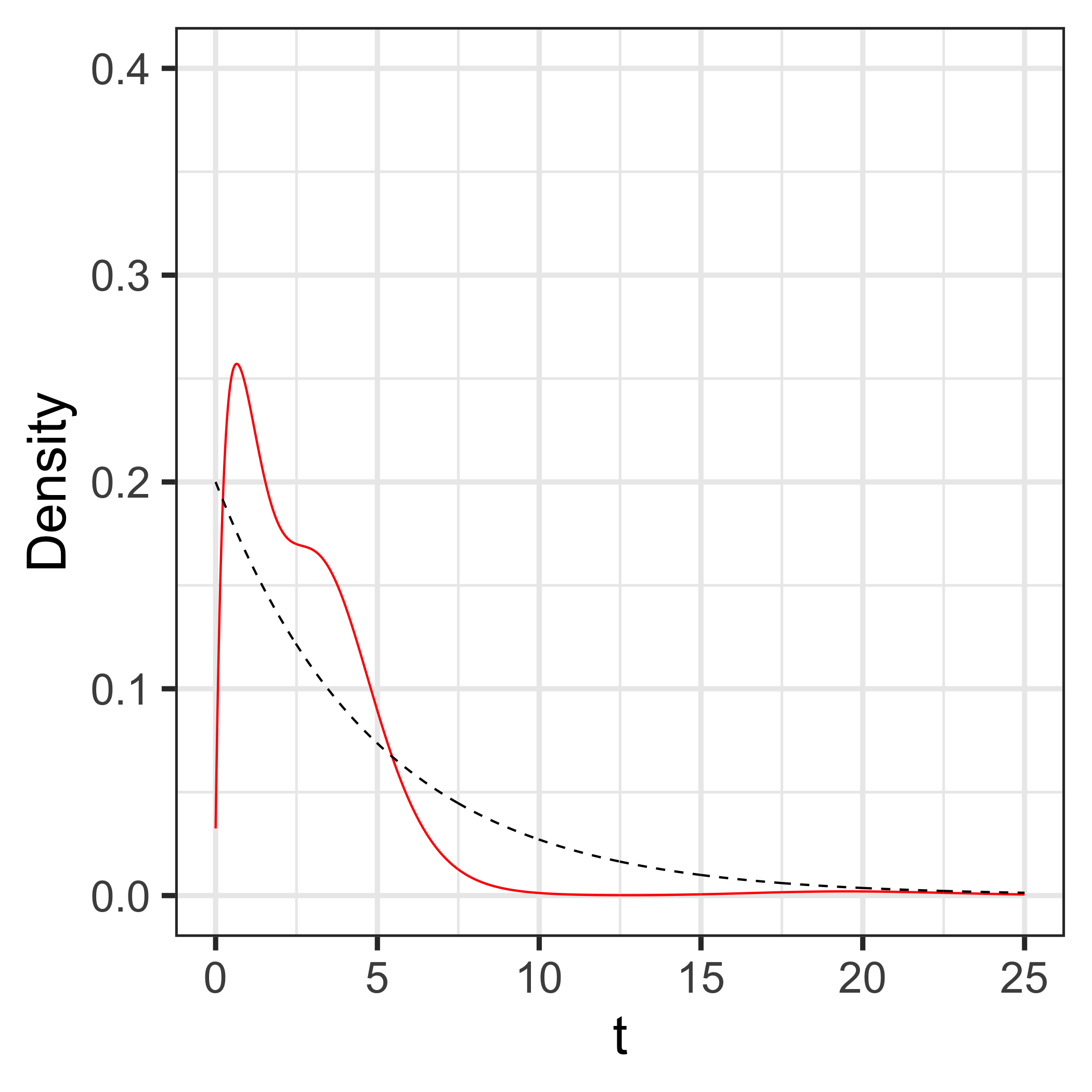
Figure 1: Prior realizations of the mixture weights $\bm{\omega}$ (top row) and the corresponding densities $f(t\mid M,\theta,G)$ given by the red solid lines (bottom row), under $\alpha=1,10,100$ (left, middle, right columns). In all cases, $M=50$, $\theta=0.5$, and $G_{0}=\text{Exp}(5)$. The black dotted line in the bottom row panels is the density of $G_{0}$.

Priors for $\theta$ and $M$.

Under the model construction for the mixture weights, $\theta$ controls the step size of the increments and thus how fine the discretization of $G$ is. Moreover, $\theta$ controls the location and dispersion of the Erlang basis densities in (1). With smaller $\theta$, the Erlang densities are more concentrated around their mean $m\theta$, and the discretization of $G$ becomes finer. Hence, and as the pointwise convergence result suggests, smaller $\theta$ values may be needed to accommodate non-standard density shapes. Also, the last component in (1) has mean $M\theta$ (with variance $M\theta^{2}$), and thus the effective support of $f(t\mid M,\theta,G)$ is jointly determined by $M$ and $\theta$; with smaller $\theta$, a greater value of $M$ is needed to achieve the same effective support. To illustrate, Figure 2 plots five prior realizations of the Erlang mixture density for each of three combinations of $(M,\theta)$, using in all cases $\alpha=10$, and an $\text{Exp}(5)$ distribution for $G_{0}$. For panels (a) and (b), $M\theta=20$. The resulting density realizations have similar effective support, although the ones in panel (b) involve more variable shapes, as expected since the value of $\theta$ is smaller than that in panel (a). For panel (c), $M\theta=5$, resulting in noticeably smaller effective support for the realized densities relative to panels (a) and (b).

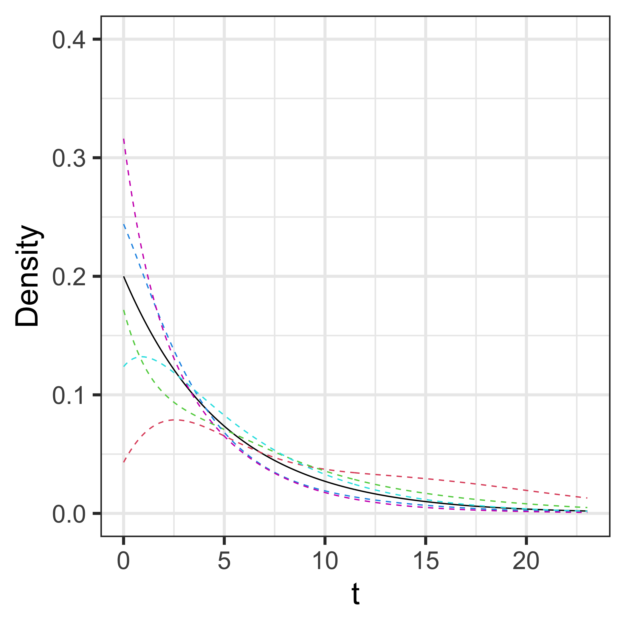
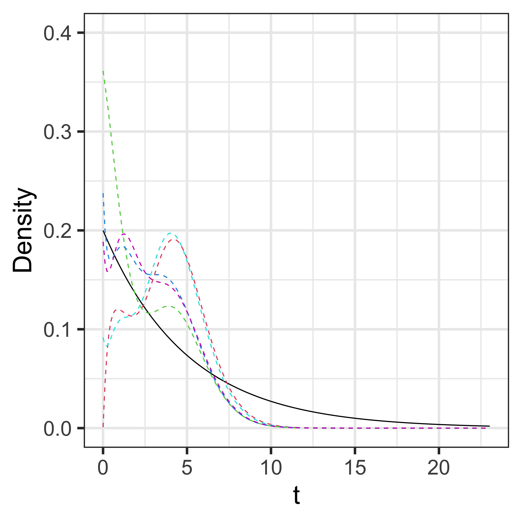
(a) $(M,\theta)=(10,2)$	(b) $(M,\theta)=(40,0.5)$	(c) $(M,\theta)=(10,0.5)$

Figure 2: Prior realizations for $f(t\mid M,\theta,G)$, under $(M,\theta)=(10,2)$, $(40,0.5)$, and $(10,0.5)$. In al cases, $\alpha=10$ and $G_{0}=\text{Exp}(5)$. The black dashed line denotes the density of $G_{0}$.

We work with a joint prior for $\theta$ and $M$, $p(\theta,M)=$ $p(\theta)p(M\mid\theta)$. We assume $\theta\sim\text{Ga}(a_{\theta},b_{\theta})$, and conditional on $\theta$, assign to $M$ a discrete uniform distribution, $M\mid\theta\sim$ $\text{Unif}(\lceil M_{1}/\theta\rceil,\dots,\lceil M_{2}/\theta\rceil)$, where $\lceil a\rceil$ is the smallest integer that is larger or equal to $a$. To specify the hyperparameters $a_{\theta}$, $b_{\theta}$, $M_{1}$ and $M_{2}$, we use a relatively conservative approach, based on the range of the data. For $M_{1}$, we choose a value greater than the largest value in the data, and set $M_{2}=$ $cM_{1}$ for a relatively small integer $c$. The motivation for this choice is to ensure that the effective support of the Erlang mixture model is sufficiently large for the particular data application. To specify the prior hyperparameters for $\theta$, we notice that $M_{1}/\theta\sim\text{inv-Ga}(a_{\theta},M_{1}/b_{\theta})$, based on which we recommend selecting values for $a_{\theta}$ and $b_{\theta}$ such that $\text{E}(M_{1}/\theta)$ is between 10 and 50.

Posterior Simulation.

The data point for the $i^{th}$ subject is recorded as $y_{i}=$ $\min(t_{i},c_{i})$, where $t_{i}$ is the survival time and $c_{i}$ the (independent) administrative censoring time, for $i=1,\ldots,n$. The data set can be represented through ${\cal D}=$ $\{(y_{i},\nu_{i}):i=1,\ldots,n\}$, where the $\nu_{i}$ are binary censoring indicators such that $\nu_{i}=1$ if $t_{i}$ is observed, and $\nu_{i}=0$ otherwise. Then, the likelihood function can be written as

$$L(M,\theta,G;{\cal D})=\prod_{i=1}^{n}\left\{f(y_{i}\mid M,\theta,G)\right\}^{\nu_{i}}\left\{S(y_{i}\mid M,\theta,G)\right\}^{1-\nu_{i}},$$ (4)

where $f(\cdot\mid M,\theta,G)\equiv$ $f(\cdot\mid M,\theta,\bm{\omega})$ and $S(\cdot\mid M,\theta,G)$ are given in (1) and (2), respectively.

We implement posterior inference via Markov chain Monte Carlo (MCMC) simulation, using standard posterior simulation methods for DP mixture models (e.g., Escobar & West, 1995; Neal, 2000). The Erlang mixture density in (1) can be expressed as a DP mixture by exploiting the definition of the weights $\omega_{m}$ through distribution $G$, resulting in the following alternative mixture representation:

$$f(t\mid M,\theta,G)\,=\,\sum_{m=1}^{M}\omega_{m}\,\text{Ga}(t\mid m,\theta)\,=\,\int_{0}^{\infty}\left\{\sum_{m=1}^{M}\mathbbm{1}_{B_{m}}(\phi)\,\text{Ga}(t\mid m,\theta)\right\}\text{d}G(\phi).$$

Here, $\mathbbm{1}_{B}(\cdot)$ is the indicator function for set $B$, and, as before, $B_{m}=$ $((m-1)\theta,m\theta]$, for $m=1,\ldots,M-1$, and $B_{M}=$ $((M-1)\theta,\infty)$.

For posterior simulation, we augment the likelihood in (4) with subject-specific latent variables, $\phi_{i}\mid G\overset{i.i.d.}{\sim}G$, which indicate the mixture component for the associated observations. In particular, if $\phi_{i}$ falls into interval $B_{m}$, the $i^{th}$ observation corresponds to the $m^{th}$ Erlang basis density. The posterior distribution involves $G$, $M$, $\theta$, the set of latent variables $\bm{\phi}=$ $\{\phi_{i}:i=1,...,n\}$, and the DP hyperparameters $(\alpha,\zeta)$. We marginalize $G$ over its DP prior and work with the prior full conditionals for the $\phi_{i}$, implied by the DP Pólya urn representation (Blackwell & MacQueen, 1973), to sample from the marginal posterior distribution for all model parameters except $G$. To this end, we employ the MCMC method in Escobar & West (1995); the details are given in Appendix A.

Although we do not sample the mixture weights $\bm{\omega}$ during the MCMC simulation, it is straightforward to obtain posterior samples for $\bm{\omega}$, using their definition in terms of distribution $G$. The conditional posterior distribution for $G$, given $(\alpha,\zeta)$ and $\bm{\phi}$, is characterized by a DP with updated total mass parameter $\alpha^{\star}=$ $\alpha+n$, and centering distribution $G_{0}^{\star}=$ $\alpha(\alpha+n)^{-1}\text{Exp}(\zeta)+(\alpha+n)^{-1}\sum_{i=1}^{n}\delta_{\phi_{i}}$. Hence, using the DP definition, the conditional posterior distribution for $\bm{\omega}$, given $M$, $(\alpha,\zeta)$, and $\bm{\phi}$, is a Dirichlet distribution with parameter vector $(\alpha^{\star}G_{0}^{\star}(B_{1}),\ldots,\alpha^{\star}G_{0}^{\star}(B_{M}))$.

Two points about the posterior simulation method are worth making. First, note that the model parameters do not explicitly contain the vector of mixture weights. The mixture weights are estimated through the posterior distribution of $G$, which plays the role of the relevant parameter. This is practically important in that the dimension of the parameter space does not change with $M$, and we thus do not need to resort to more complex trans-dimensional MCMC algorithms. Second, the DP-based Erlang mixture model offers an interesting example where full posterior inference can be obtained from a DP mixture model without the need to truncate or approximate the DP prior. This is a result of the use of a marginal MCMC method, as well as of the fact that distribution $G$ enters the model only through increments of its distribution function, which define the mixture weights.

2.2 Model extension for control-treatment studies

A practically relevant scenario in studies where survival responses are collected involves data from multiple experimental groups, typically associated with different treatments. Evidently, it is of interest in these settings to compare survival distributions across different groups. We develop an extension of the Erlang mixture model in this direction, focusing on the case of two groups for, say, a generic control-treatment study. Our objective is to retain the flexible modeling approach for the survival distributions, avoiding restrictions to specific parametric shapes or rigid relationships, such as proportional hazards. We also seek a prior probability model that allows for dependence, and thus borrowing of information, between the two distributions.

We use the dependent DP (DDP) prior structure (MacEachern, 2000) that extends the DP prior for distribution $G$ to a prior model for a collection of covariate-dependent distributions, $G_{x}$, where $x$ indexes the distributions in terms of values in the covariate space. Our context involves a binary covariate $x\in\mathcal{X}=$ $\{C,T\}$, where $C$ and $T$ represent control and treatment groups, respectively. The DDP prior builds from the DP stick-breaking representation (Sethuraman, 1994) by utilizing covariate-dependent weights and/or atoms. We work with a common-weights DDP prior model:

$$G_{x}\,=\,\sum_{\ell=1}^{\infty}p_{\ell}\,\delta_{\varphi^{*}_{x\ell}},~{}~{}~{}\mbox{ for }x\in{\cal X},$$ (5)

with $p_{1}=v_{1}$, $p_{\ell}=v_{\ell}\prod_{r=1}^{\ell-1}(1-v_{r})$, for $\ell\geq 2$, where the $v_{\ell}$ are i.i.d. from a $\text{Beta}(1,\alpha)$ distribution, and the atoms $\bm{\varphi}^{\star}_{\ell}=$ $(\varphi^{\star}_{{\mbox{\tiny C}}\ell},\varphi^{\star}_{{\mbox{\tiny T}}\ell})$ arise i.i.d. from a bivariate distribution $G_{0}$. Note that, under this construction, $G_{x}$ follows marginally a $\mbox{DP}(\alpha,G_{0x})$ prior, where $G_{0x}$, for $x\in{\cal X}$, are the marginals of $G_{0}$ associated with the control and treatment groups. For $G_{0}$, we consider a bivariate log-normal distribution, such that $\bm{\varphi}^{\star}_{\ell}\mid\bm{\mu}\overset{i.i.d.}{\sim}\mbox{LN}_{2}(\bm{\mu},\Sigma)$, with $\Sigma$ specified. We place a bivariate normal, $\text{N}_{2}(\bar{\bm{\mu}},\Sigma_{0})$, hyperprior on $\bm{\mu}$, with $\bar{\bm{\mu}}$ and $\Sigma_{0}$ fixed, and a gamma hyperprior on the total mass parameter $\alpha$.

Allowing also for group-specific number of Erlang basis densities, $M_{x}$, as well as group-specific Erlang scale parameter, $\theta_{x}$, the extension of the Erlang mixture model in (1) can be expressed as

$$f_{x}(t)\,\equiv\,f(t\mid M_{x},\theta_{x},G_{x})\,=\,\sum_{m=1}^{M_{x}}\omega_{xm}\,\text{Ga}(t\mid m,\theta_{x}),~{}~{}~{}t\in\mathbbm{R}^{+},$$ (6)

where $\omega_{xm}=G_{x}(m\theta_{x})-G_{x}((m-1)\theta_{x})$, $m=1,\ldots,M_{x}-1$, and $\omega_{xM_{x}}=1-G_{x}((M_{x}-1)\theta_{x})$. Similar to the model in (1), the group-specific Erlang basis densities are fully specified given $M_{x}$ and $\theta_{x}$. Furthermore, the survival functions, $S_{x}(t)$, and hazard functions, $h_{x}(t)$, under the extended model have a mixture representation similar to (2) and (3),

$$S_{x}(t)\,=\,\sum_{m=1}^{M_{x}}\omega_{xm}\,S_{{\tiny\text{Ga}}}(t\mid m,\theta_{x})~{}~{}~{}\mbox{ and }~{}~{}~{}h_{x}(t)\,=\,\sum_{m=1}^{M_{x}}\omega_{xm}^{\star}(t)\,h_{{\tiny\text{Ga}}}(t\mid m,\theta_{x}),$$ (7)

where $\omega_{xm}^{\star}(t)=\omega_{xm}\,S_{{\tiny\text{Ga}}}(t\mid m,\theta_{x})/\{\sum_{m^{\prime}=1}^{M_{x}}\omega_{xm^{\prime}}\,S_{{\tiny\text{Ga}}}(t\mid m^{\prime},\theta_{x})\}$. Note that both the mixture components and weights are indexed by $x$. Again, the time-dependent weights in the hazard mixture form allow for local adjustment, and thus for flexible group-specific hazard rate shapes. Importantly, the prior model allows for general relationships between the control and treatment group hazard functions. In particular, inference is not restricted by the proportional hazards assumption, implied by several commonly used parametric or semiparametric survival regression models.

To complete the full Bayesian model, we place priors on $\theta_{x}$ and $M_{x}$, using again the role of these parameters (discussed in Section 2.1). More specifically, for each $x$, the joint prior, $p(\theta_{x},M_{x})=p(\theta_{x})p(M_{x}\mid\theta_{x})$. We further assume $\theta_{x}\overset{ind}{\sim}\text{Ga}(a_{x\theta},b_{x\theta})$, and $M_{x}\mid\theta_{x}\overset{ind.}{\sim}\text{Unif}\left(\left\lceil M_{x1}/\theta_{x}\right\rceil,\dots,\left\lceil M_{x2}/\theta_{x}\right\rceil\right)$. We use an approach similar to the one described in Section 2.1 to specify $M_{x1}$ and $M_{x2}$, and the hyperparameters for $\theta_{x}$.

Posterior simulation for the DDP-based Erlang mixture model proceeds with a relatively straightforward extension of the MCMC simulation method in Section 2.1. The details are provided in Appendix B.

The primary focus of this paper is on the DP-based Erlang mixture model for survival analysis and its extension for the control-treatment setting. We note however that the DDP-based Erlang mixture model can be further extended to accommodate a general $p$-variate covariate vector $\bm{x}$. For example, we may consider a linear-DDP structure (De Iorio et al., 2009) to extend $G_{x}$ in (5) to $G_{\bm{x}}=$ $\sum_{\ell=1}^{\infty}p_{\ell}\,\delta_{\psi^{\star}_{\ell}(\bm{x})}$, where $\psi^{\star}_{\ell}(\bm{x})=\exp((1,{\bm{x}}^{\prime})\bm{\beta}_{\ell})$ with the $\bm{\beta}_{\ell}$ i.i.d. from a baseline distribution. The structured DDP prior for $G_{\bm{x}}$ yields covariate-dependent mixture weights, and thus a nonparametric prior model for covariate-dependent survival densities and hazard functions. A regression model may also be used for $M$ and/or $\theta$. Different from the linear-DDP mixture of log-normal distributions in De Iorio et al. (2009), the extended model retains the parsimonious Erlang mixture structure.

3 Simulation Study

We use three simulation scenarios to illustrate the models developed in Section 2. For the Erlang mixture model for a single distribution, we consider simulated data from: a two-component log-normal mixture to demonstrate the model’s capacity to estimate non-standard density and hazard function shapes (Section 3.1); and, a log-normal distribution sampled with different levels of censoring (Section 3.2). The DDP-based extension of the model is illustrated in Section 3.3 with a synthetic data example based on a log-normal control distribution and a two-component log-normal mixture treatment distribution, specified such that the corresponding hazard functions cross each other.

For all data examples considered here and in Section 4, we used the approach discussed in Section 2 to specify the prior hyperparameters. Consistent with inference results obtained from DP mixture models, we have observed some sensitivity to the prior choice for $\alpha$. The effect on the posterior distribution for $\alpha$ is more noticeable for the small cell lung cancer data of Section 4.2 (involving the smallest sample size among our data examples). However, posterior inference results for survival functionals are largely unaffected even under fairly different priors for $\alpha$. When the sample size is relatively small for each group, we recommend applying the DDP-based Erlang mixture model with a prior for $\alpha$ that supports small to moderate values, such as the $\text{Ga}(5,1)$ prior used in Section 3.3 and 4.2.

We examined convergence and mixing of the MCMC algorithms using standard diagnostic techniques. In our experiments, we observed that parameters $\theta$ and $M$ are highly correlated, and moderate thinning was used to improve efficiency. A general approach we take is to run the MCMC chain for 100,000 iterations, then discard the first 25% posterior samples and keep every 38th iteration for posterior inference.

3.1 Example 1: Bimodal density

We simulate $n=200$ survival times from a mixture of two log-normal distributions, $0.4\,\text{LN}(1,0.4)+0.6\,\text{LN}(2,0.2)$, which yields a bimodal density and a non-monotonic hazard function. The true underlying functions $f(t)$, $S(t)$ and $h(t)$ are plotted in Figure 3. Regarding prior specification, we used: $\alpha\sim\text{Ga}(2,1)$; $\zeta\sim\text{inv-Ga}(3,4)$; $\theta\sim\text{Ga}(1,1)$; and, $M\mid\theta\sim\text{Unif}\left(\left\lceil M_{1}/\theta\right\rceil,\dots,\left\lceil M_{2}/\theta\right\rceil\right)$, with $M_{1}=13$ and $M_{2}=$ $3\times M_{1}$.

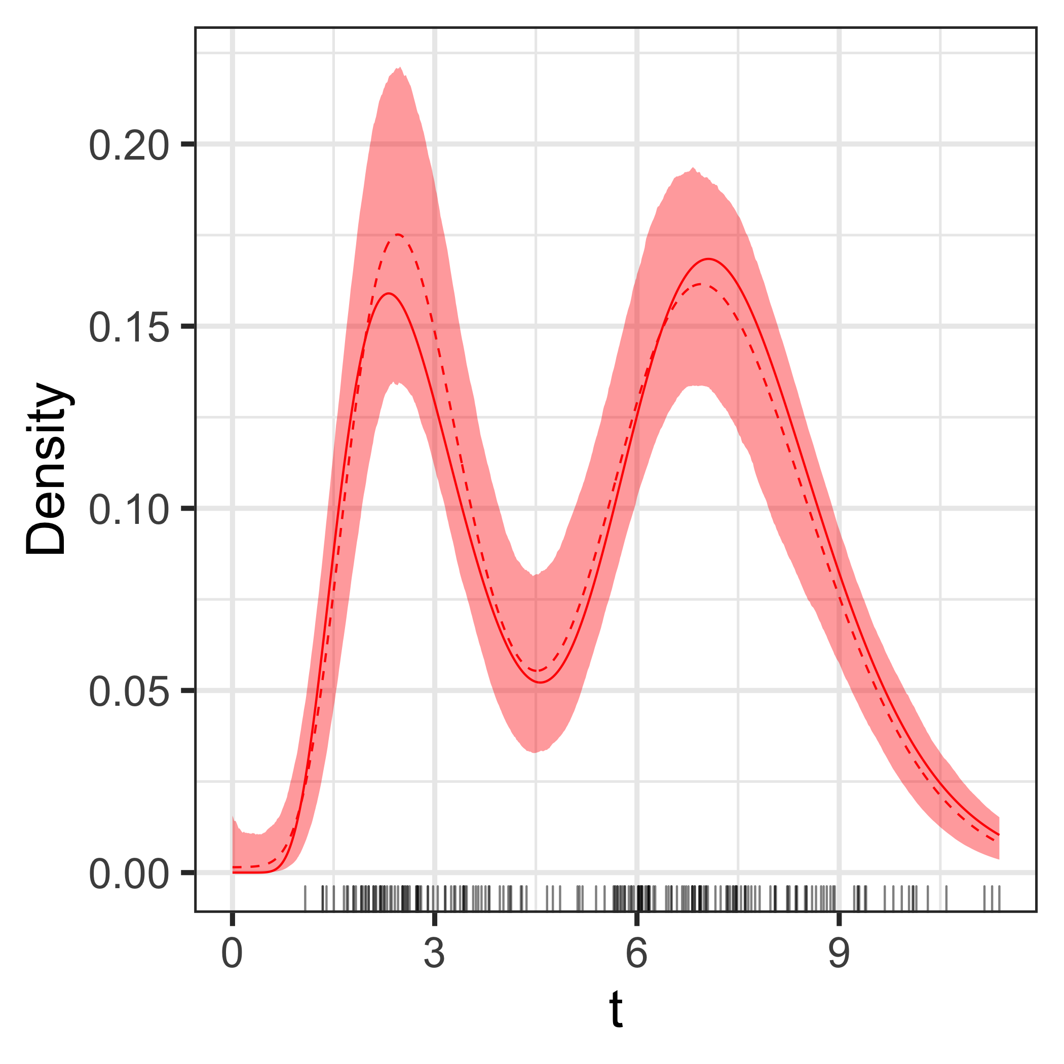
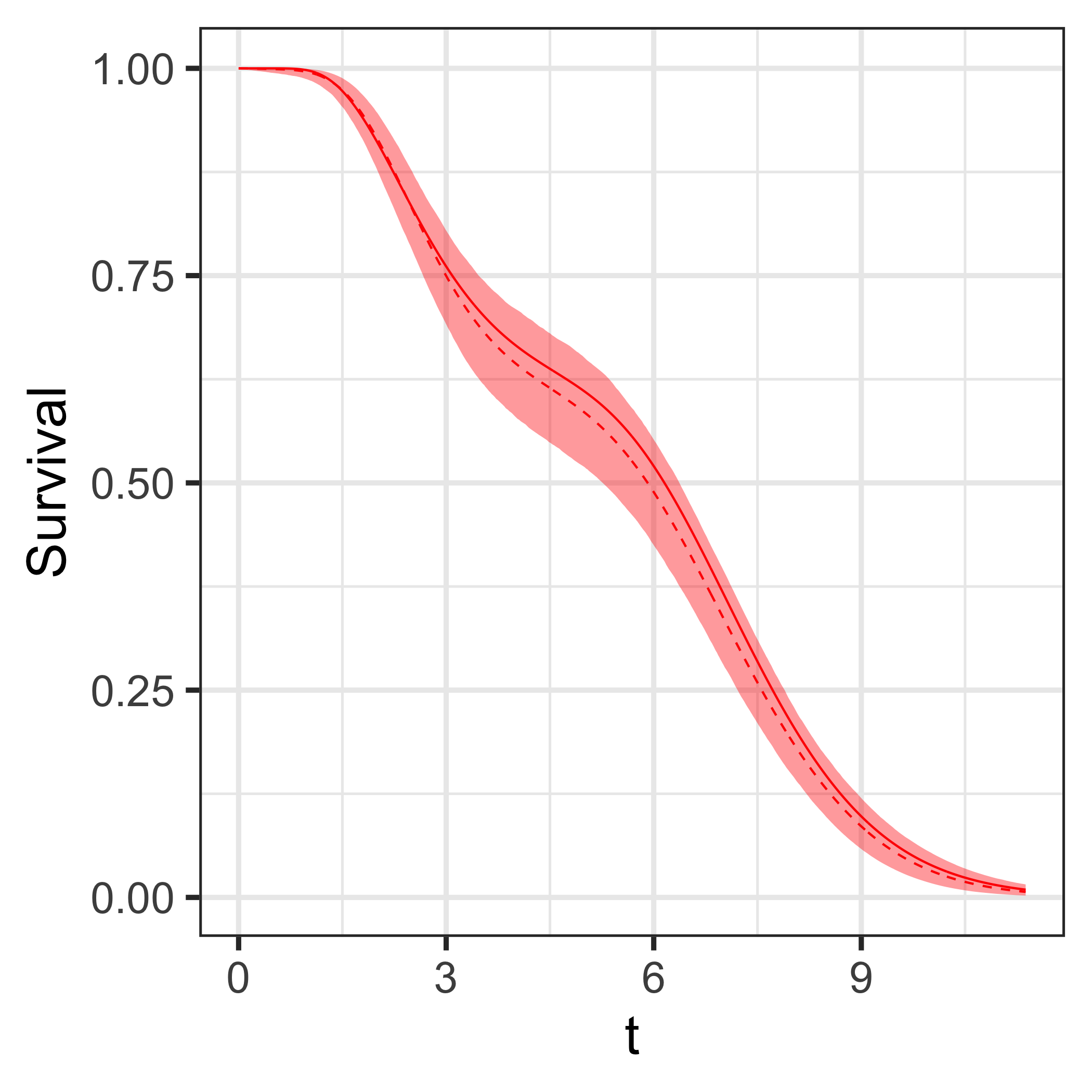
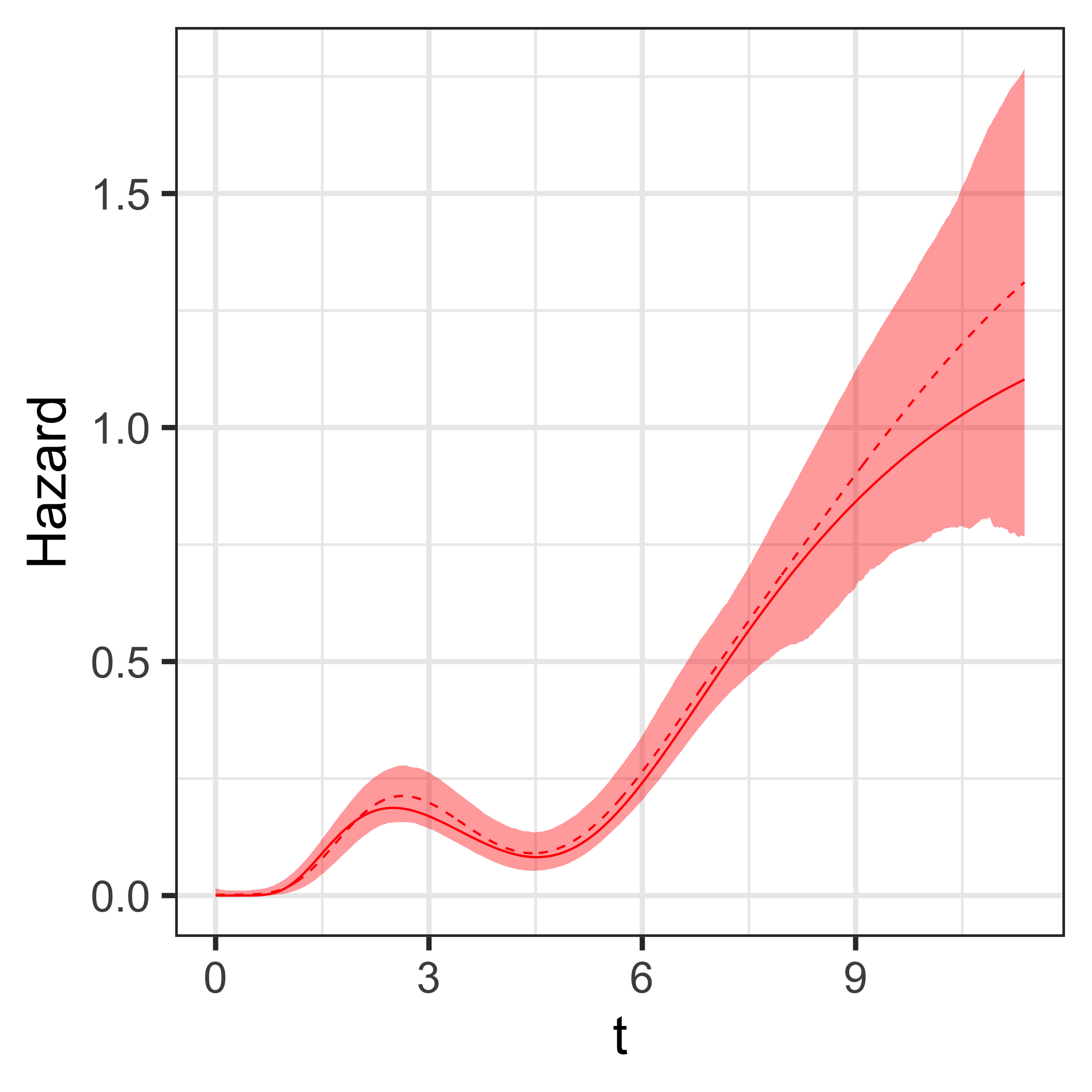
(a) Density function	(b) Survival function	(c) Hazard function

Figure 3: Simulation Example 1. Posterior mean (dashed lines) and 95% interval estimates (shaded regions) for the density function (left panel), survival function (middle panel) and hazard function (right panel). The red solid line in each panel corresponds to the true underlying function. The black marks on the x-axis in the left panel show the observed survival times.

Posterior inference is summarized in Figure 3. The complex features of the underlying survival functionals are captured well by the model. In particular, the inference results for the hazard function demonstrate the effectiveness of the model structure in (3) with the time-dependent weights allowing for local adjustment and estimation of a non-standard hazard function shape.

The posterior distribution for the common scale parameter $\theta$ is substantially concentrated on smaller values relative to its prior, in particular, the posterior mean and 95% credible interval estimates for $\theta$ are $0.28$ and $(0.13,0.39)$. Recalling the definition of the mixture weights, this indicates the level of partitioning needed to accommodate the non-standard, bimodal shape of the underlying density. The posterior mean and 95% credible interval estimates of the number $M$ of mixture components are $101$ and $(44,223)$. However, the number of effective mixture components (i.e., effective basis densities) is considerably smaller than $M$. As an informal rule, we identify an effective Erlang basis density through its corresponding mixture weight taking value greater than a threshold of $0.01$. Then, the number of effective mixture components is about $4$ (on average across posterior samples). For a graphical illustration, Figure 4 plots three randomly selected posterior realizations of $f(t\mid M,\theta,G)$. The associated posterior draws for $(\theta,M)$ are $(0.2,153)$, $(0.33,78)$, and $(0.25,54)$, whereas the number of effective Erlang basis densities is only $4$, $2$, and $5$, respectively. The weighted effective basis densities (i.e., $\omega_{m}\times\text{Ga}(t\mid m,\theta)$ for $m$ such that $\omega_{m}>0.01$) are also plotted in Figure 4. This example highlights the critical importance of the nonparametric prior for distribution $G$ that defines the weights for the Erlang mixture model.

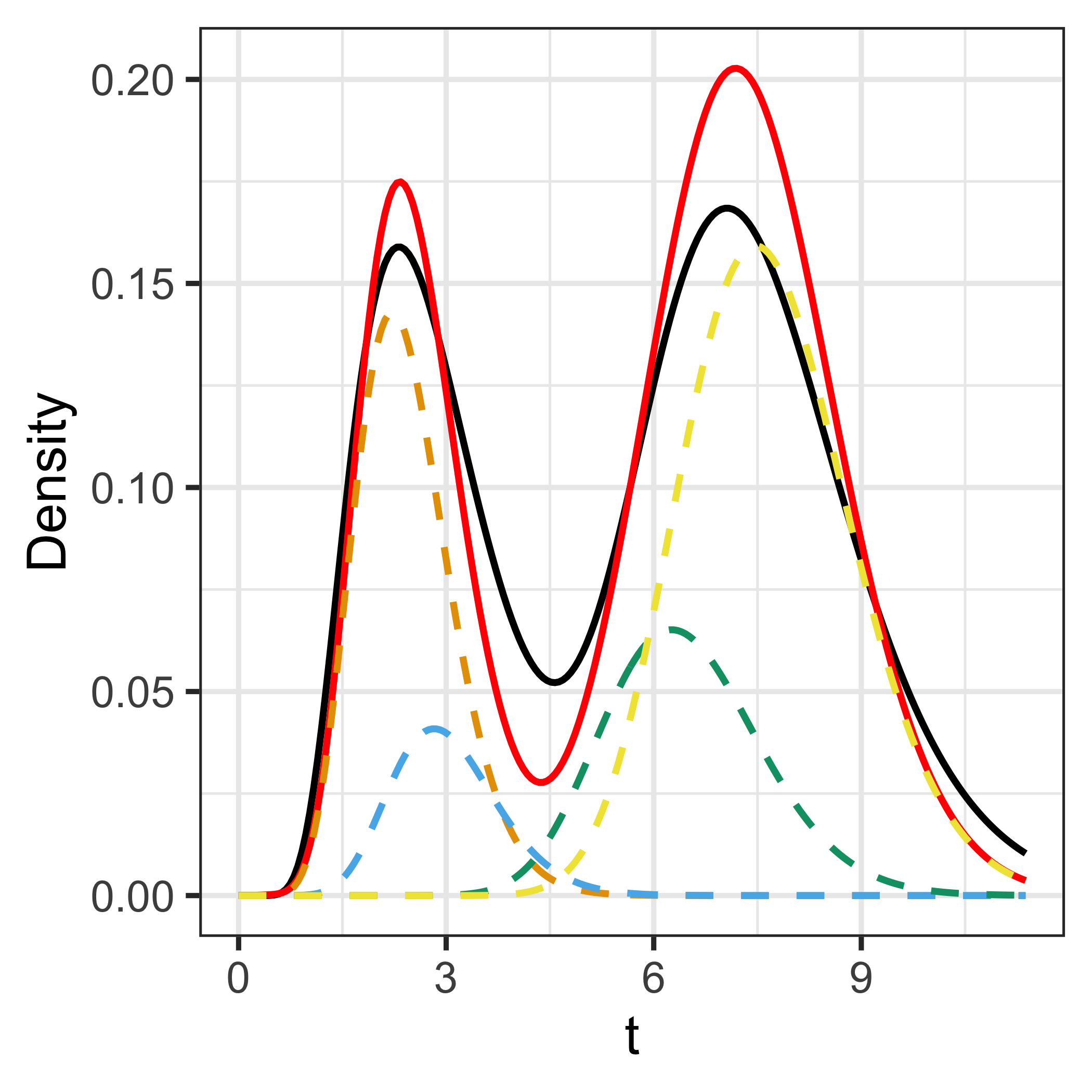
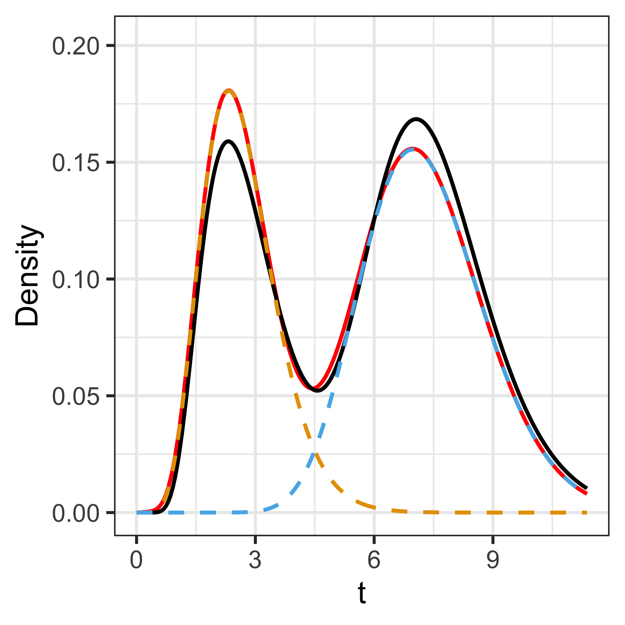
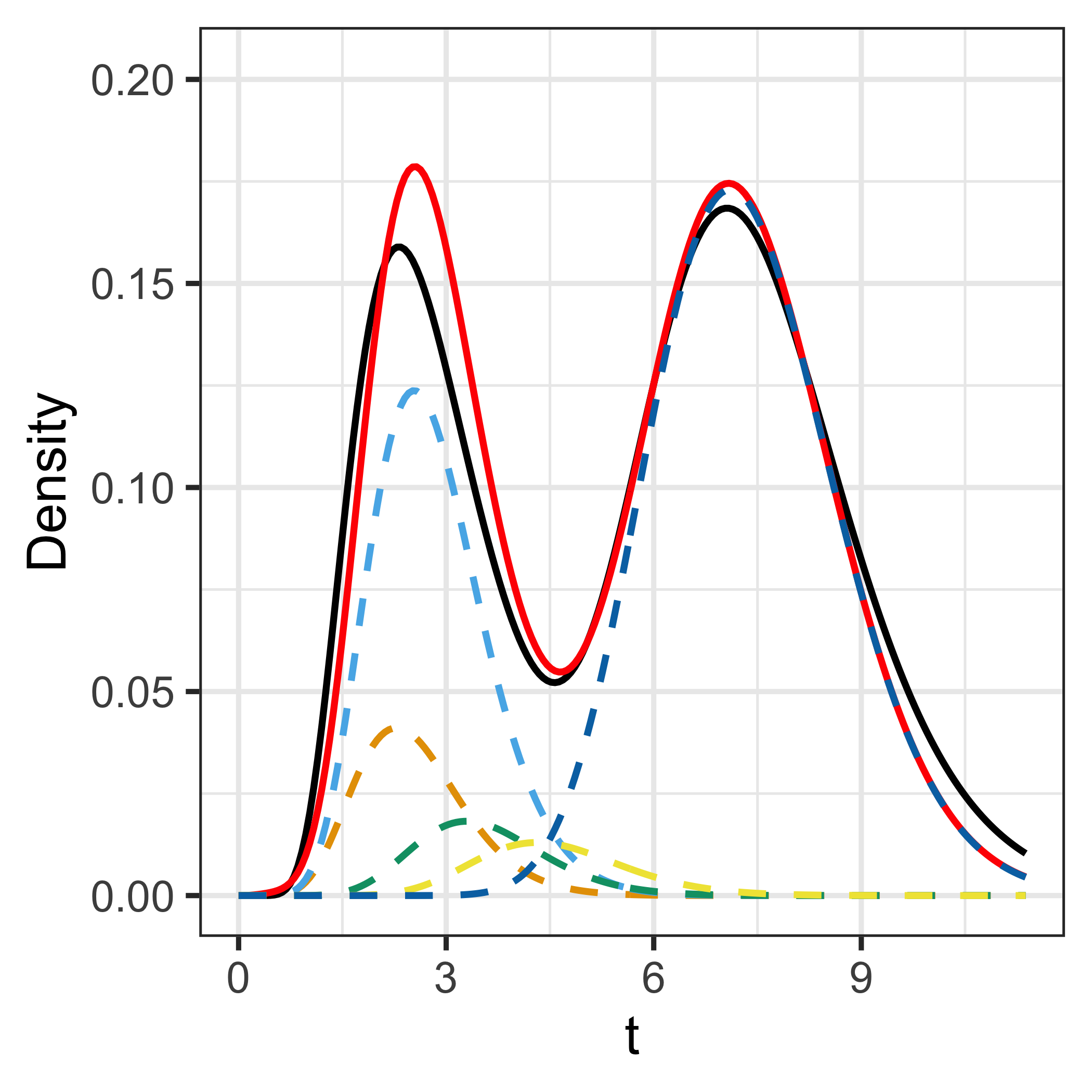
(a) $\theta=0.20$, $M=153$	(b) $\theta=0.33$, $M=78$	(c) $\theta=0.25$, $M=54$

Figure 4: Simulation Example 1. Plots (a)-(c) show the posterior realization of $f(t\mid M,\theta,G)$ (red solid line), based on three randomly chosen posterior samples. Each dashed line represents the Erlang basis density $\text{Ga}(t\mid m,\theta)$ for components with $\omega_{m}>0.01$, multiplied by its corresponding weight. The black solid line is the true underlying density.

(a) Density function	(b) Survival function	(c) Hazard function

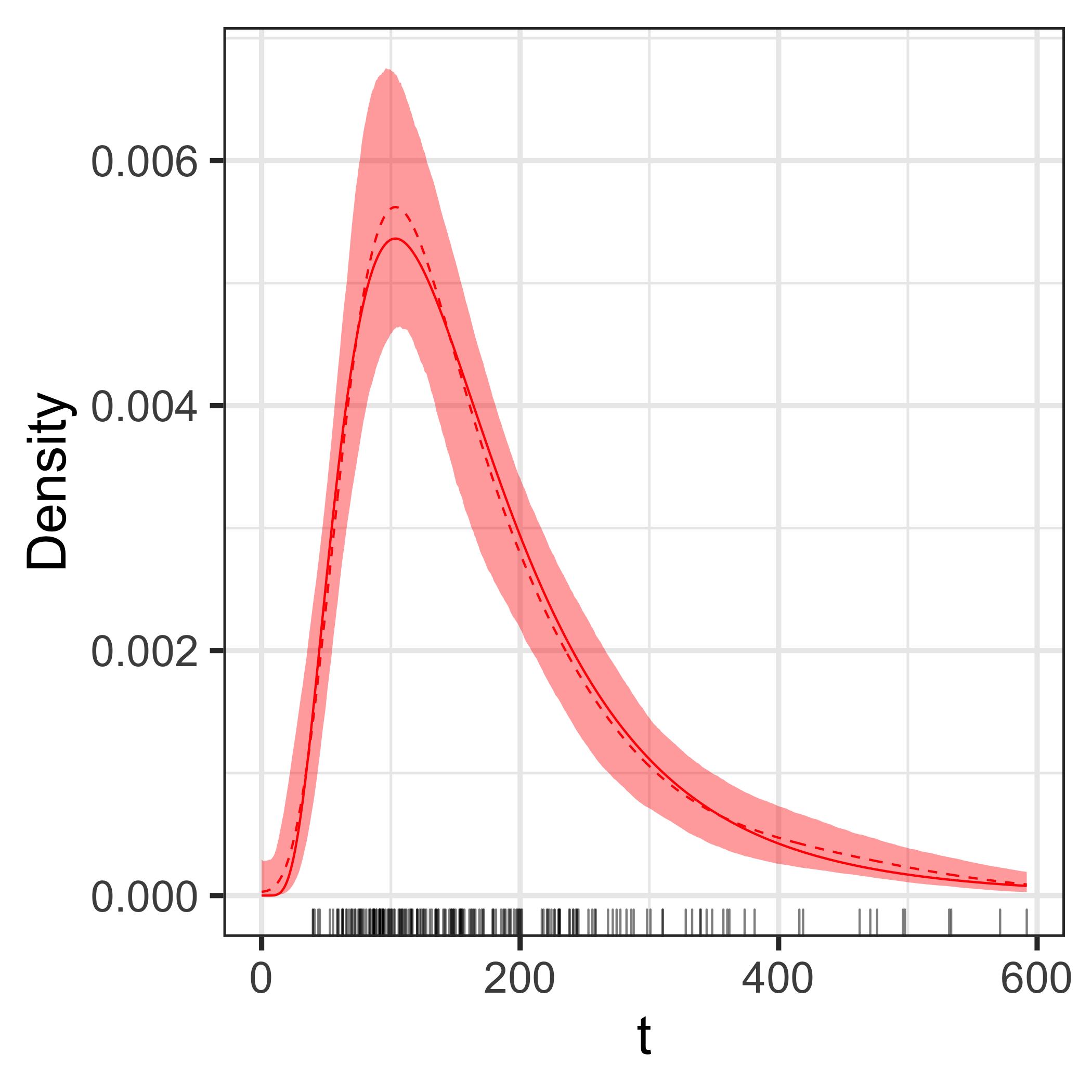
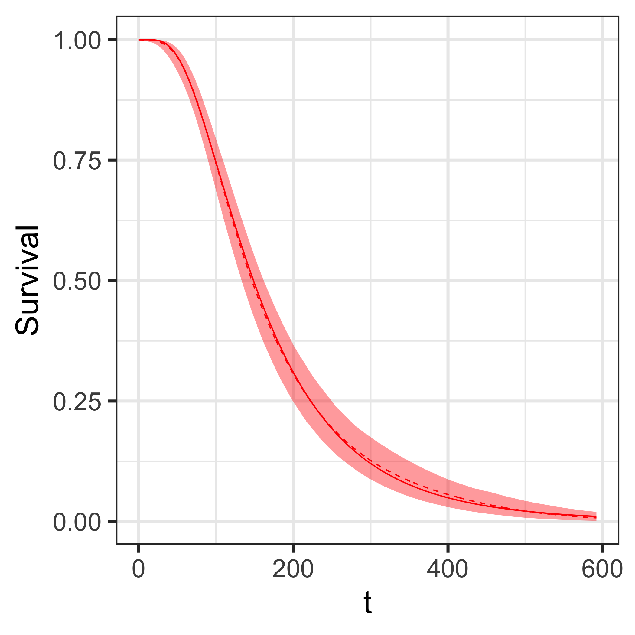
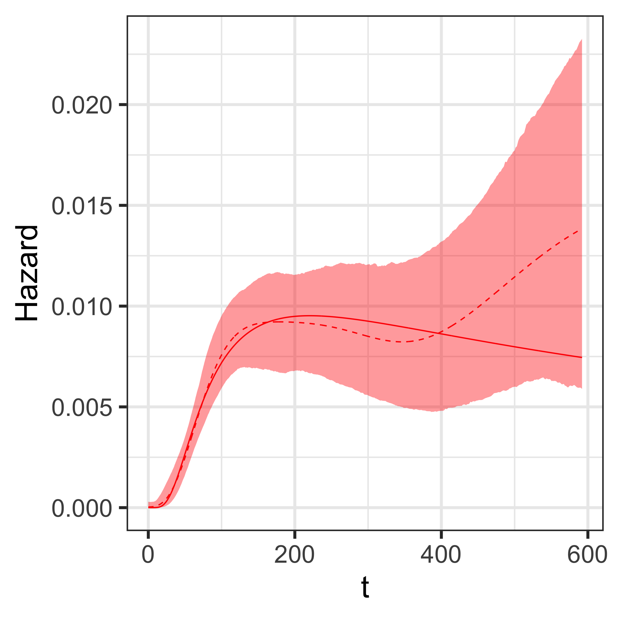
Figure 5: Simulation Example 2 (data without censoring). Posterior mean (dashed lines) and 95% interval estimates (shaded regions) for the density function (left panel), survival function (middle panel) and hazard function (right panel). The red solid line in each panel corresponds to the true underlying function, and the black rugs in the left panel show the survival times.

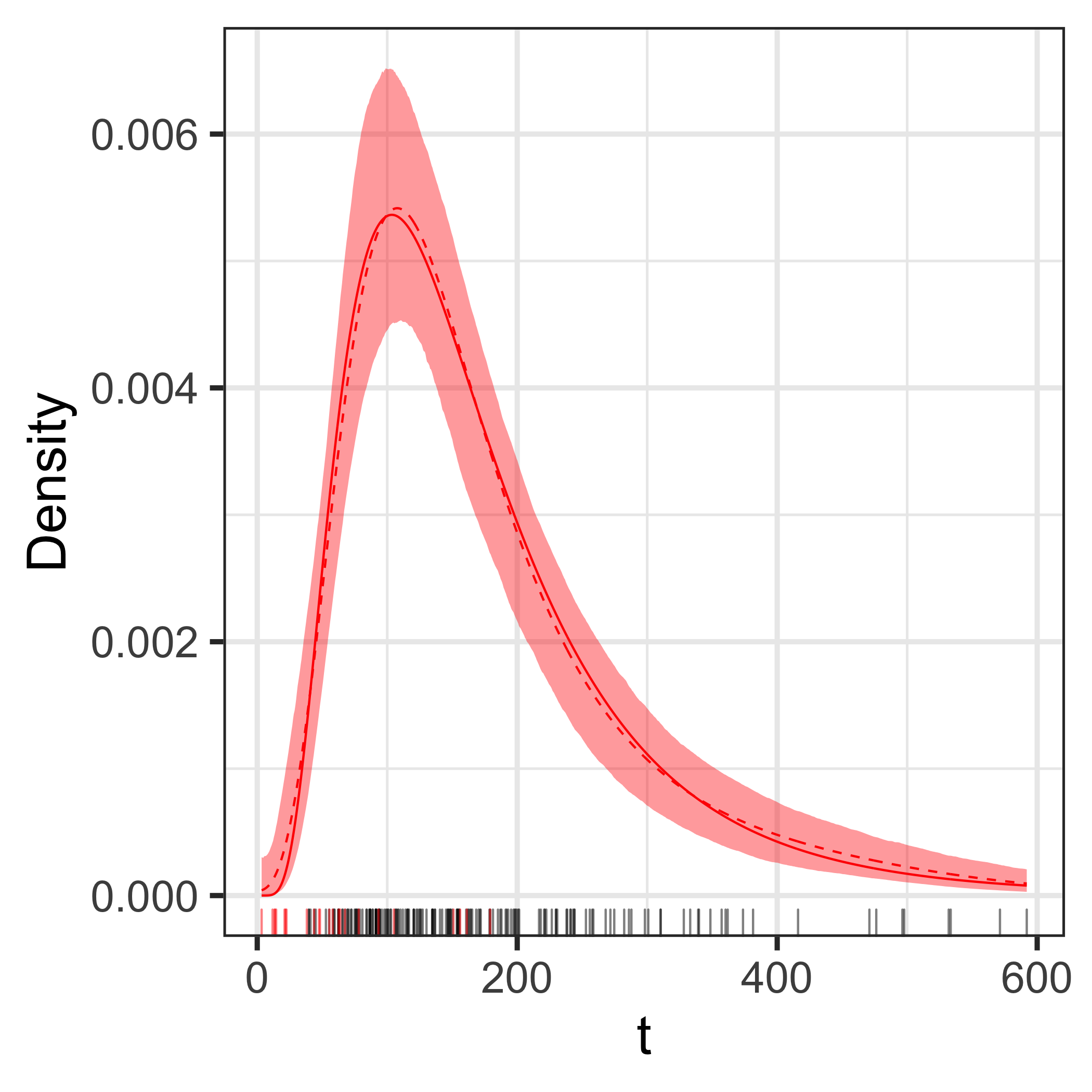
(a) Density, $g=12\%$

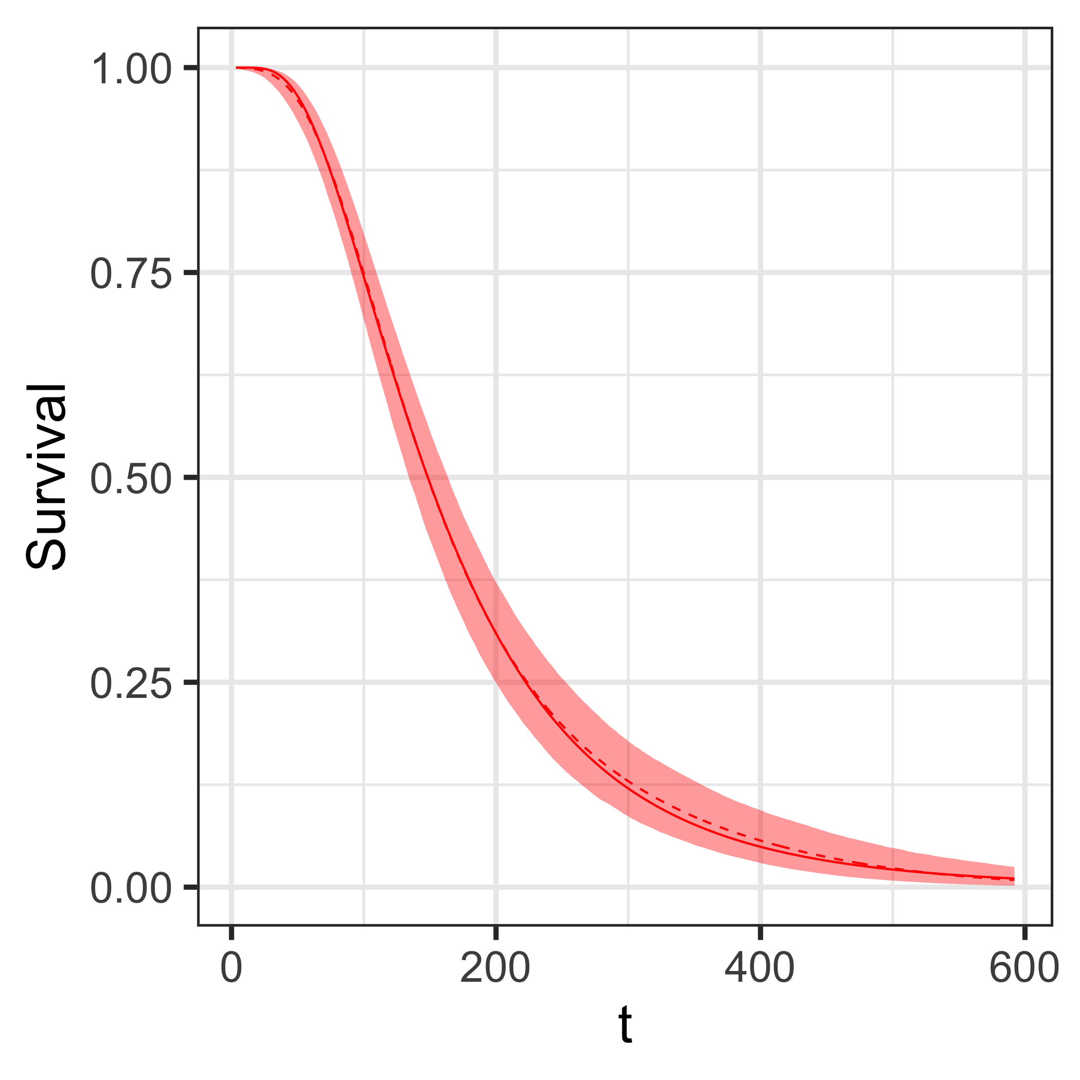
(b) Survival $g=12\%$

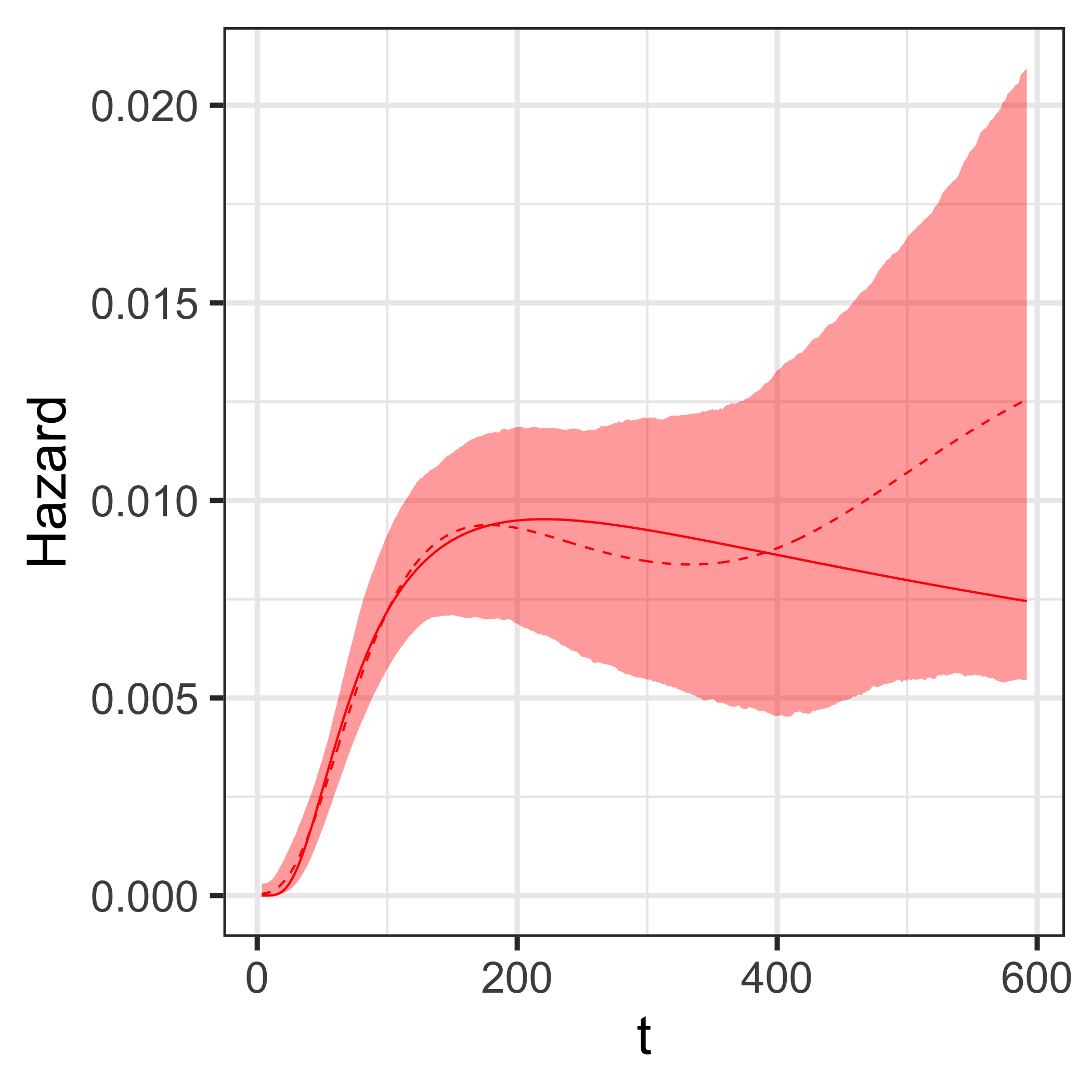
(c) Hazard, $g=12\%$

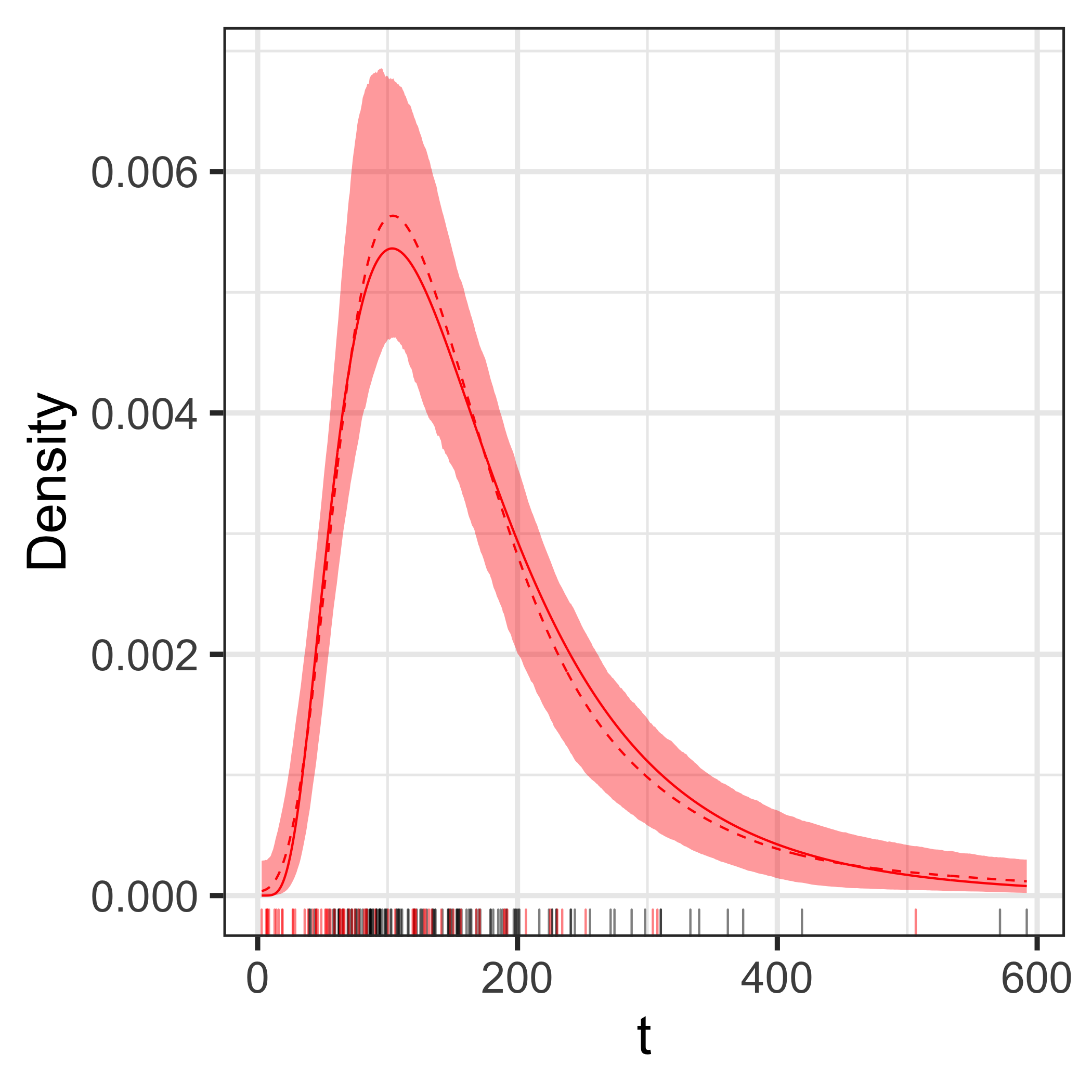
(d) Density, $g=33.5\%$

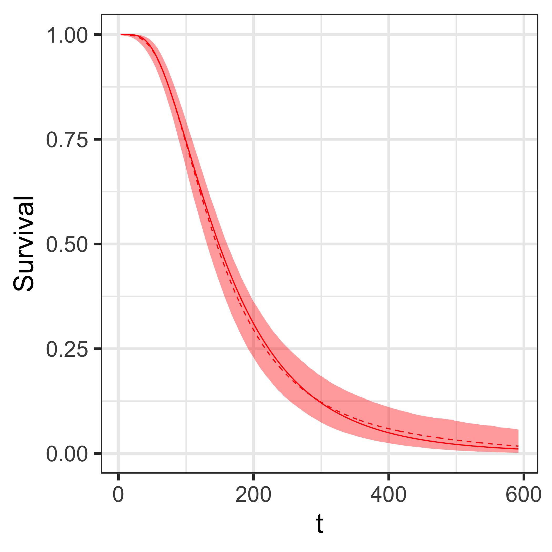
(e) Survival, $g=33.5\%$

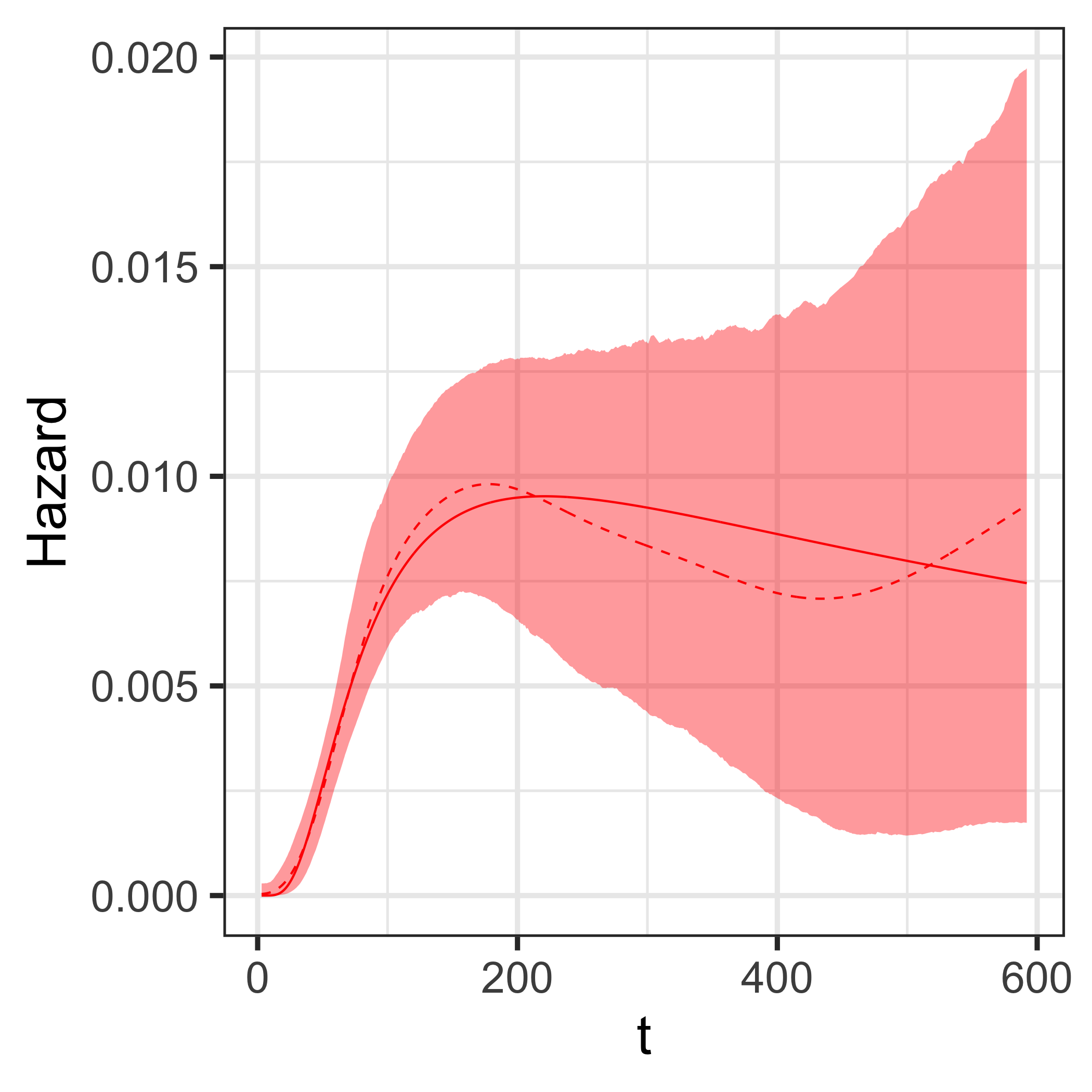
(f) Hazard, $g=33.5\%$

Figure 6: Simulation Example 2 (censored data). Posterior mean (dashed lines) and 95% interval estimates (shaded regions) for the density function (left column), survival function (middle column) and hazard function (right column). The top and bottom row corresponds to the data with censoring proportion $g=$ 12% and 33.5%, respectively. The red solid line in each panel denotes the true underlying function. The rug plots in the left column panels indicate the data points, where the black and red marks correspond to observed and censored survival times, respectively.

3.2 Example 2: Unimodal density with censoring

For the second synthetic data example, we generate survival times from a log-normal distribution, $t_{i}\overset{i.i.d.}{\sim}\text{LN}(5,0.6)$, $i=1,\ldots,n$ with $n=200$. The priors for the model parameters are: $\alpha\sim\text{Ga}(2,1)$; $\zeta\sim\text{inv-Ga}(3,1000)$; $\theta\sim\text{Ga}(2,25)$; and, $M\mid\theta\sim\text{Unif}\left(\left\lceil 1000/\theta\right\rceil,\dots,\left\lceil 3000/\theta\right\rceil\right)$.

As shown in Figure 5, the model estimates well the density, survival and hazard function. The point estimate for the hazard function is less accurate beyond $t=400$, which is to be expected given the very few observations that are greater than that time point, although the interval estimate contains the true function throughout the observation time window.

In addition, we examine the model’s performance for data with censored observations. We simulate censoring times $c_{i}$ from an exponential distribution with mean parameter $\kappa$, and define the observed times as $y_{i}=\min(t_{i},c_{i})$, with binary censoring indicators $\nu_{i}=$ $1(y_{i}\leq c_{i})$. We generate the $c_{i}$ under two different values of $\kappa$, resulting in two datasets with different proportions of censored observations, $g=$ 12% and 33.5%. Figure 6 plots posterior mean and 95% interval estimates for the density, survival and hazard functionals. We note that censoring does not substantially affect the quality of the inference results, with the true function contained in all cases within the posterior interval estimates. The width of the posterior uncertainty bands increases with the larger censoring proportion, with the increase more noticeable for the hazard function estimates.

3.3 Example 3: A control-treatment synthetic data set

Here, we examine the performance of the DDP-based Erlang mixture model of Section 2.2. We consider a binary covariate, $x_{i}=C$ or $T$, with 100 responses in each group, such that $n=200$. We generate $t_{i}\overset{i.i.d.}{\sim}\text{LN}(5,0.6)$ for subjects with $x_{i}=C$, and $t_{i}\overset{i.i.d.}{\sim}0.4\,\text{LN}(5,0.4)$ + $0.6\,\text{LN}(6,0.2)$ for subjects with $x_{i}=T$. The true density, survival and hazard functions are shown in Figure 7. The control group density is unimodal, whereas the treatment group has a bimodal density and a non-standard, non-monotonic hazard function. The truth is specified such that we have crossing hazard functions for the two groups, a scenario that traditional proportional hazards models can not accommodate.

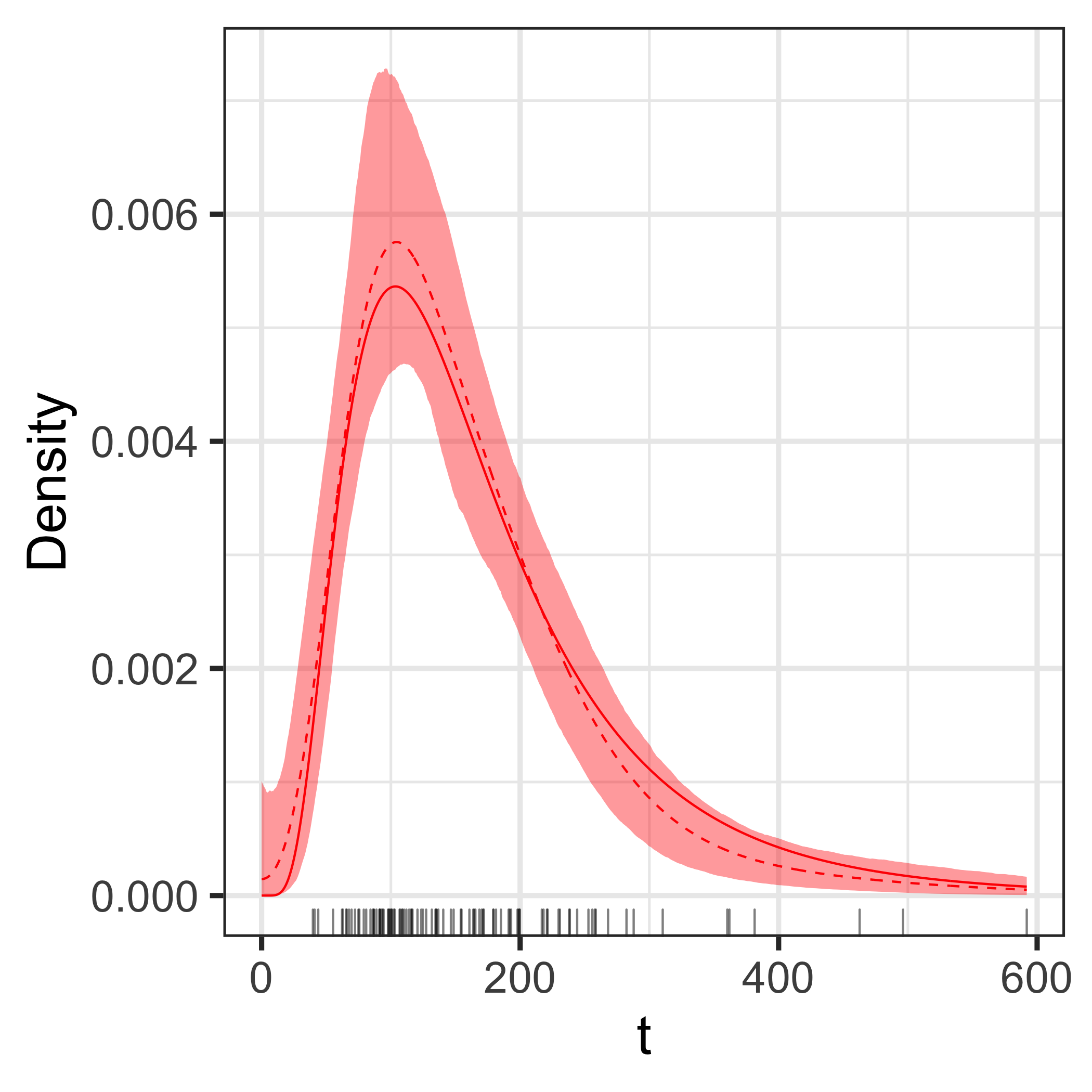
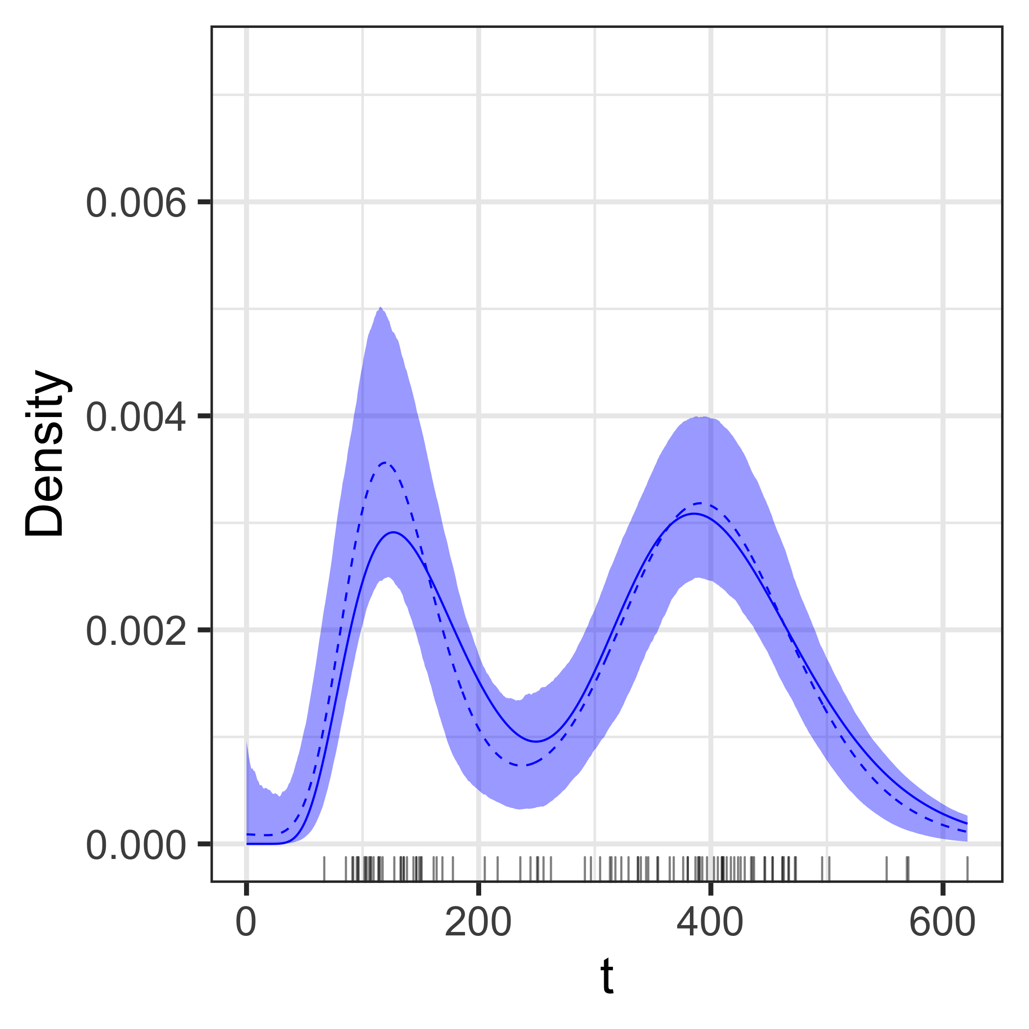
(a) Density (control group)	(b) Density (treatment group)
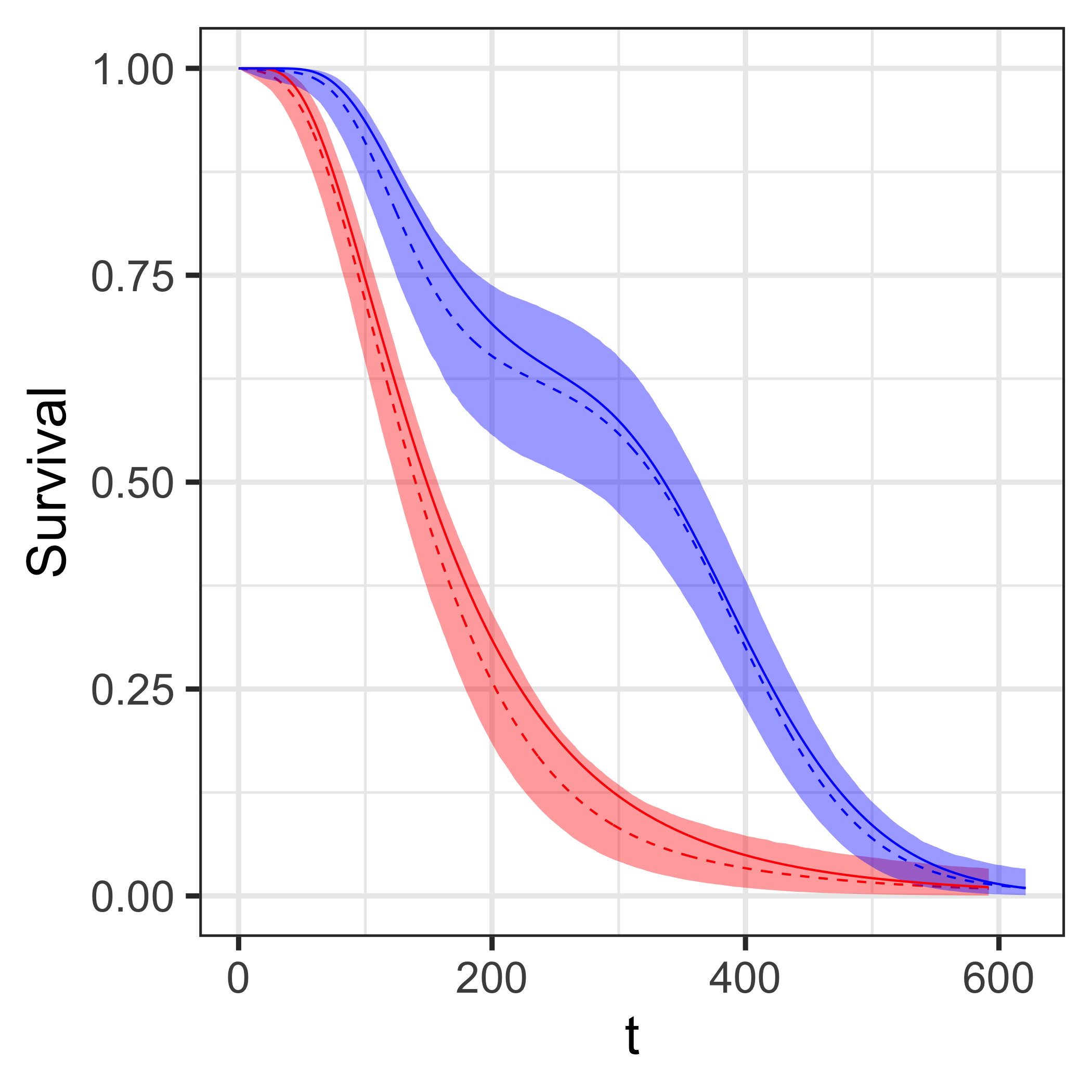
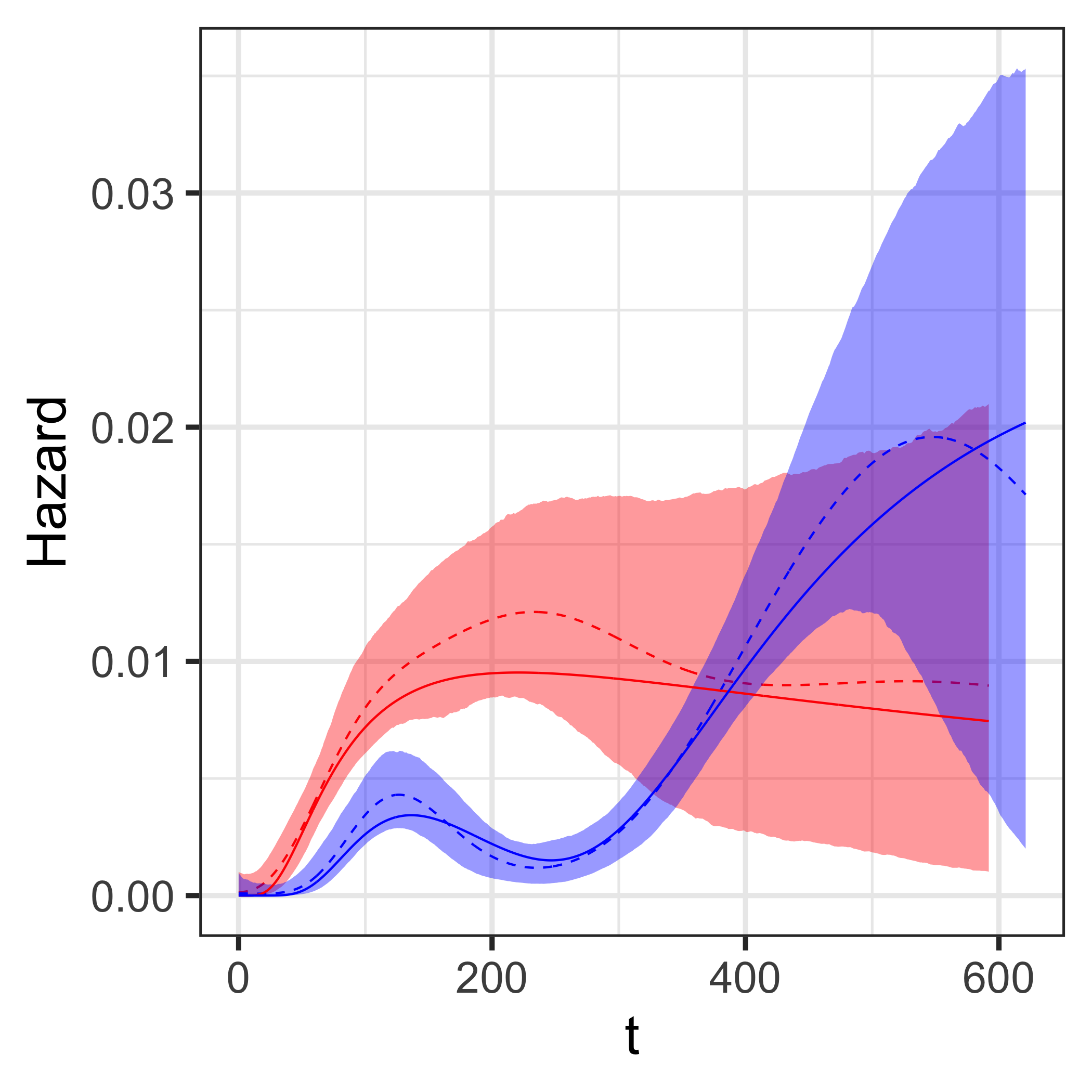
(c) Survival function	(d) Hazard function

Figure 7: Simulation Example 3. Panels (a) and (b) plot the estimates for the control and treatment group density, respectively (the rug plots show the corresponding survival times). Panels (c) and (d) compare the estimates for the survival and hazard function, respectively. In each panel, the dashed lines denote the posterior mean estimates, the solid line the true underlying function, and the shaded regions indicate the 95% credible intervals. Red and blue color is used for the control and treatment group, respectively.

Regarding the prior hyperparameters, we set: $\alpha\sim\text{Ga}(5,1)$; $\bm{\mu}\sim\text{N}_{2}((5,5.5)^{\prime},10\,\mbox{I}_{2})$; $\Sigma=3\,\mbox{I}_{2}$; $\theta_{x}\overset{ind.}{\sim}\text{Ga}(2,50)$; and, $M_{x}\mid\theta_{x}\overset{ind.}{\sim}$ $\text{Unif}\left(\left\lceil 1000/\theta_{x}\right\rceil,\dots,\left\lceil 4000/\theta_{x}\right\rceil\right)$. As shown in Figure 7, the model captures effectively the shape of the survival functionals, despite the fact that the functions vary greatly across the two groups, and it successfully recovers the non-proportional hazards relationship between the groups. Again, with respect to hazard estimation, the point estimates are generally less accurate and the interval bands are wider for larger time points where data is scarce.

4 Data Examples

4.1 Liver metastases data

We consider data on survival times (in months) from 622 patients with liver metastases from a colorectal primary tumor without other distant metastases, available from the R package “locfit”. The censoring proportion is high, with 259 censored responses. The data set has been used in earlier work to illustrate classical and Bayesian nonparametric methods for density and hazard estimation; see, e.g., Antoniadis et al. (1999) and Kottas (2006).

To apply the DP-based Erlang mixture model, we set the priors as follows: $\alpha\sim\text{Ga}(5,1)$; $\zeta\sim\text{inv-Ga}(3,80)$; $\theta\sim\text{Ga}(2,2)$; and, $M\mid\theta\sim\text{Unif}(\left\lceil 100/\theta\right\rceil,\dots,\left\lceil 300/\theta\right\rceil)$. Inference results for the density, survival, and hazard function are reported in Figure 8. The model estimates a unimodal survival density (with mode at about 13 months), with a non-standard, skewed right tail. The hazard rate estimate increases up to about 17 months, stays roughly constant between 17 to 35 months, and then decreases. The width of the posterior uncertainty bands for the hazard function increases considerably beyond 40 months, which is consistent with the fact that there are very few responses beyond that time point, and almost all of them are censored. Density and hazard rate estimates with similar shapes were obtained from the previous analyses in Antoniadis et al. (1999) and Kottas (2006). Overall, this example supports the findings from the simulation study regarding the Erlang mixture model’s capacity to effectively estimate non-standard density and hazard function shapes.

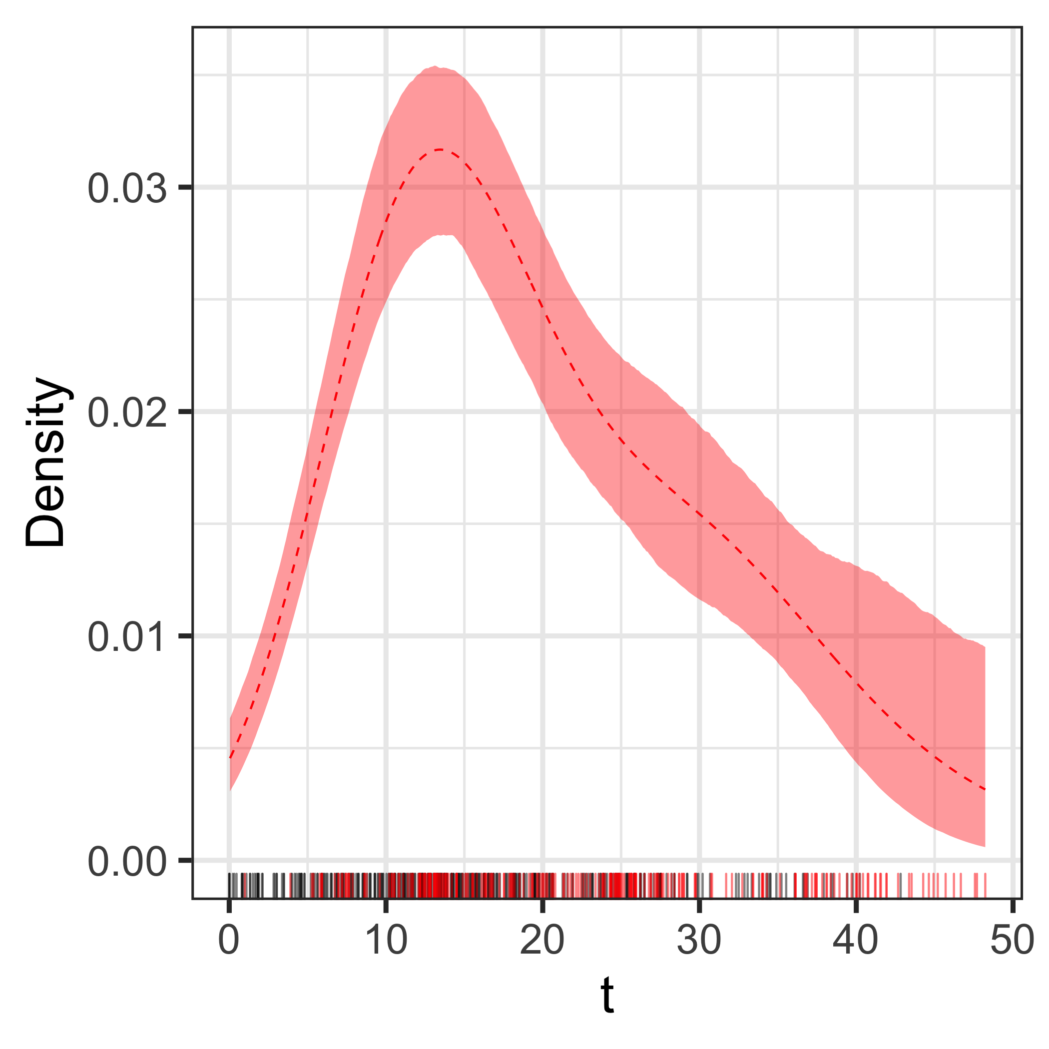
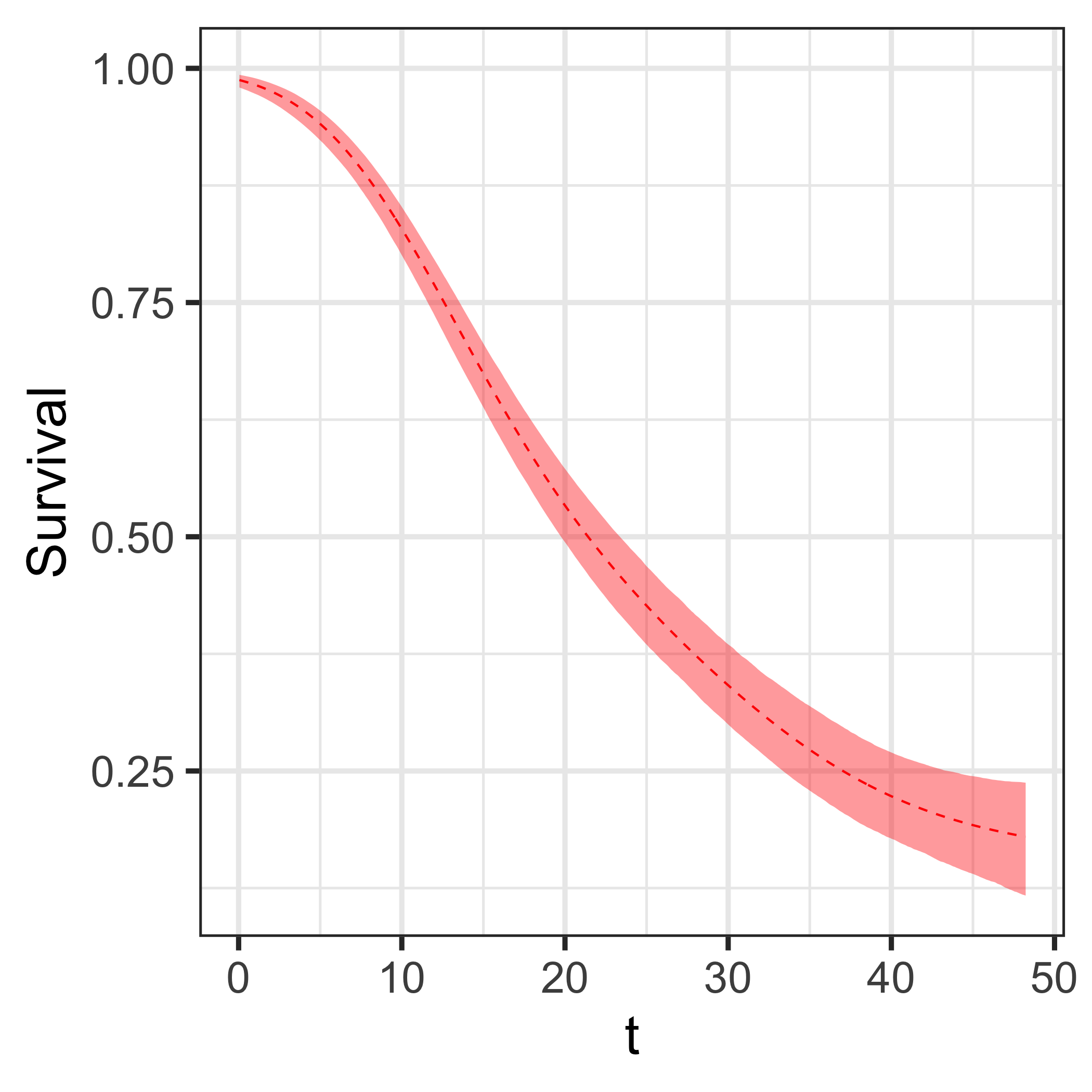
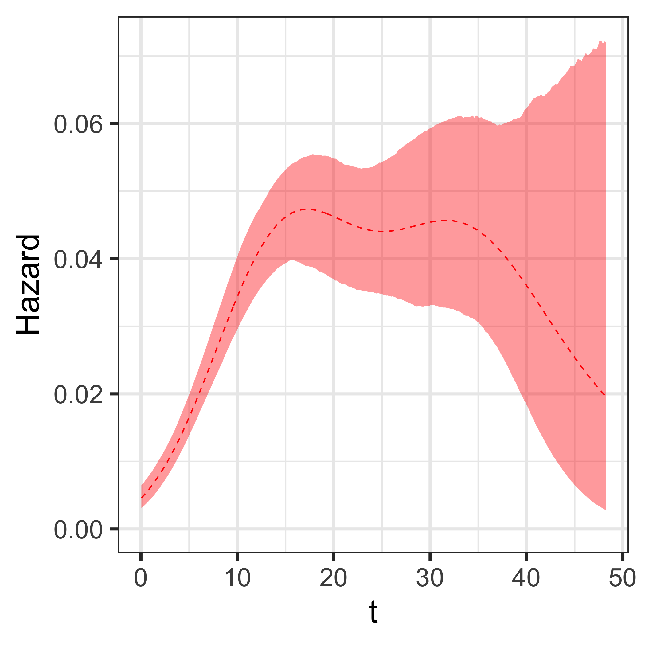
(a) Density function	(b) Survival function	(c) Hazard function

Figure 8: Liver metastases data. Panels (a), (b) and (c) plot posterior mean (dashed lines) and 95% interval estimates (shaded regions) for the density, survival and hazard function, respectively. The rug plot in panel (a) shows observed (black) and censored (red) survival times.

4.2 Small cell lung cancer data

To illustrate the DDP-based Erlang mixture model with real data, we consider the data set from Ying et al. (1995) on survival times (in days) of patients with small cell lung cancer. The data correspond to a study designed to evaluate two treatment regimens of drugs, etoposide (E) and cisplatin (P), given with a different sequence, with Arm A denoting the regimen where P is followed by E, and Arm B the regimen where E is followed by P. A total of 121 patients were randomly assigned to one of the treatment arms, resulting in 62 patients in Arm A, and 59 in Arm B. The survival times of 23 patients (15 in Arm A and 8 in Arm B) are administratively right censored.

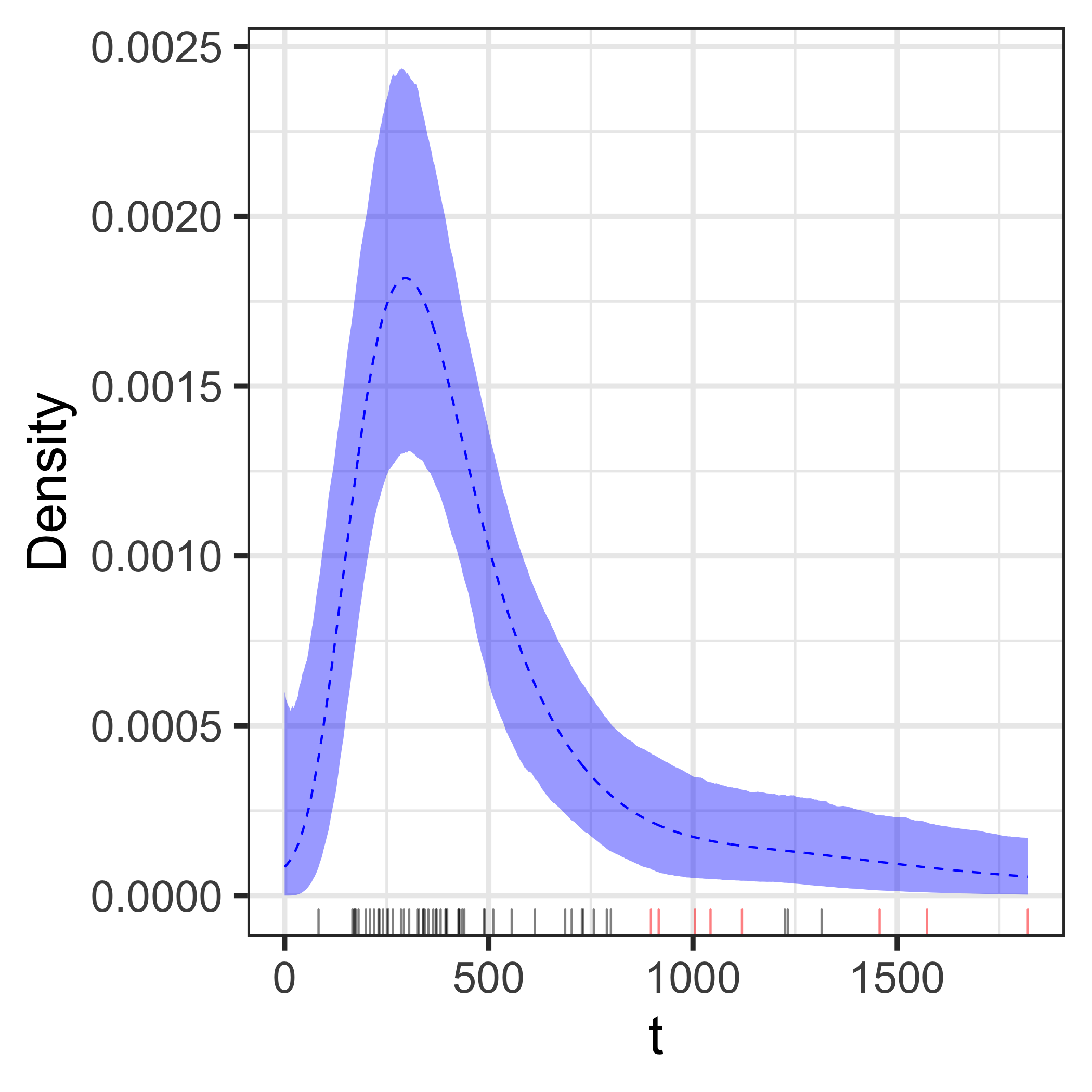
(a) Density function (Arm A)	(b) Density function (Arm B)
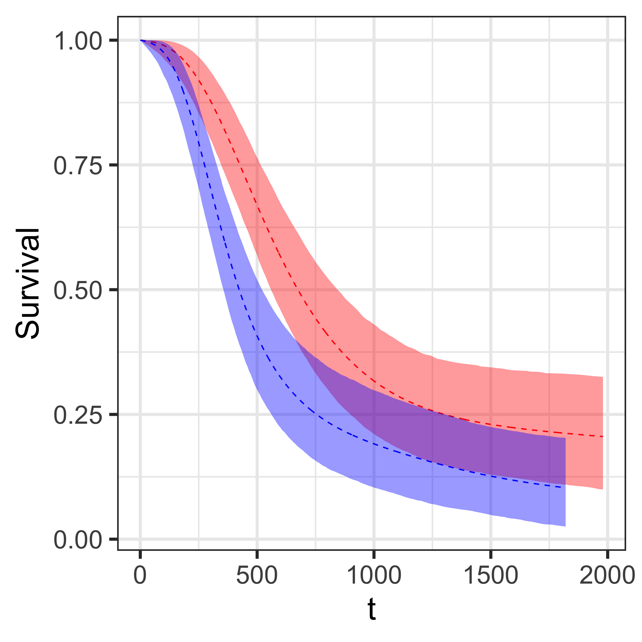
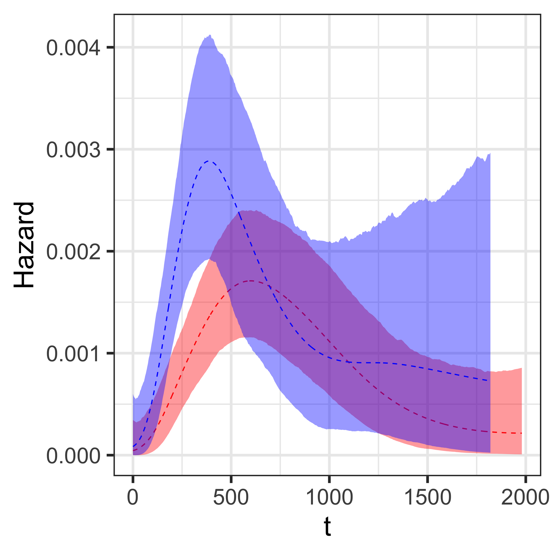
(c) Survival functions	(d) Hazard functions

Figure 9: Small cell lung cancer data. Panels (a) and (b) plot estimates for the Arm A and Arm B density; the rug plots show observed (black) and censored (red) survival times. Panels (c) and (d) compare the estimates for the survival and hazard function. In each panel, the dashed lines denote the posterior mean estimates, and the shaded regions indicate the 95% credible intervals. Red and blue color is used for the Arm A and Arm B group, respectively.

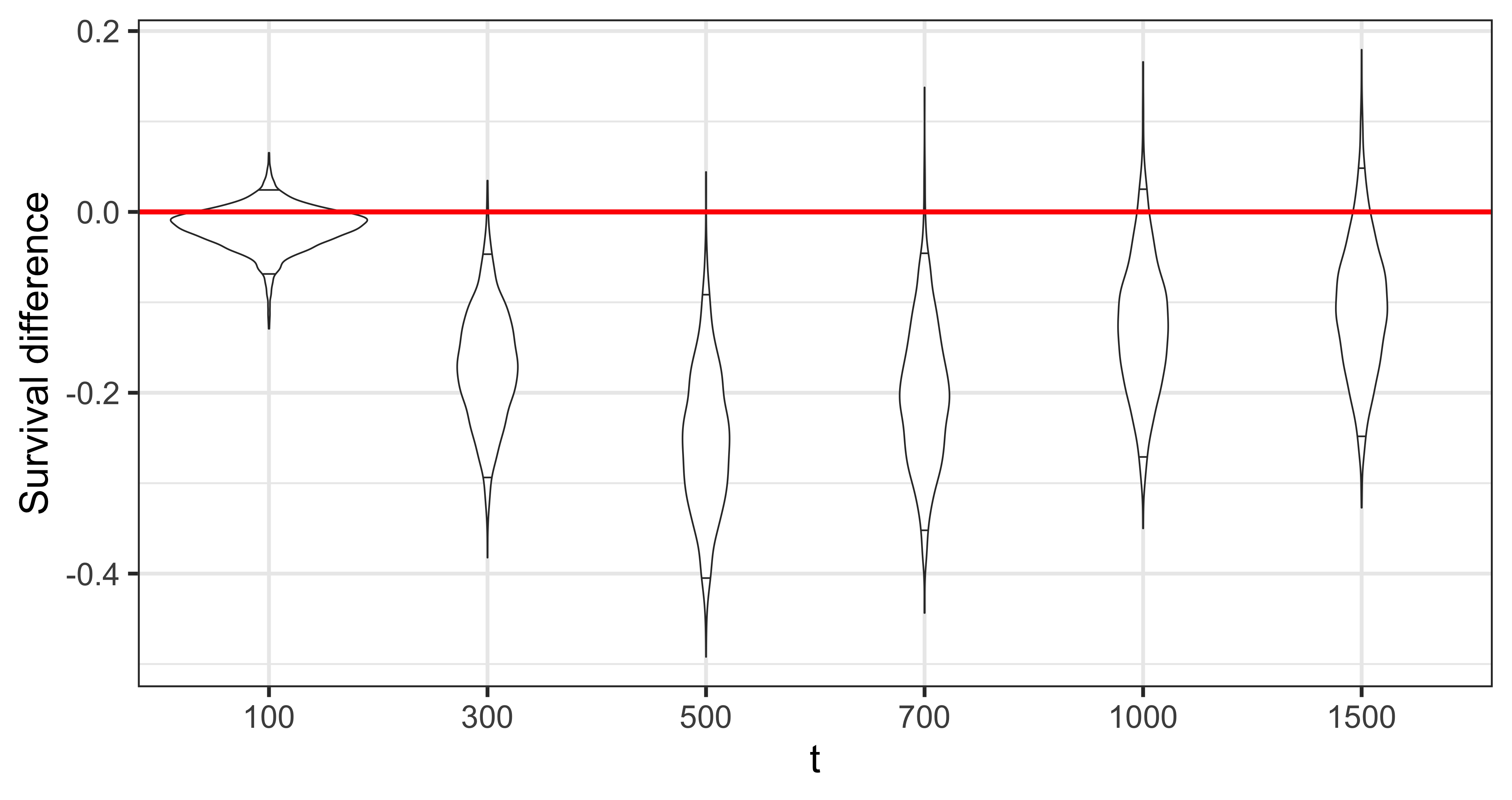
(a) $S_{B}(t)-S_{A}(t)$

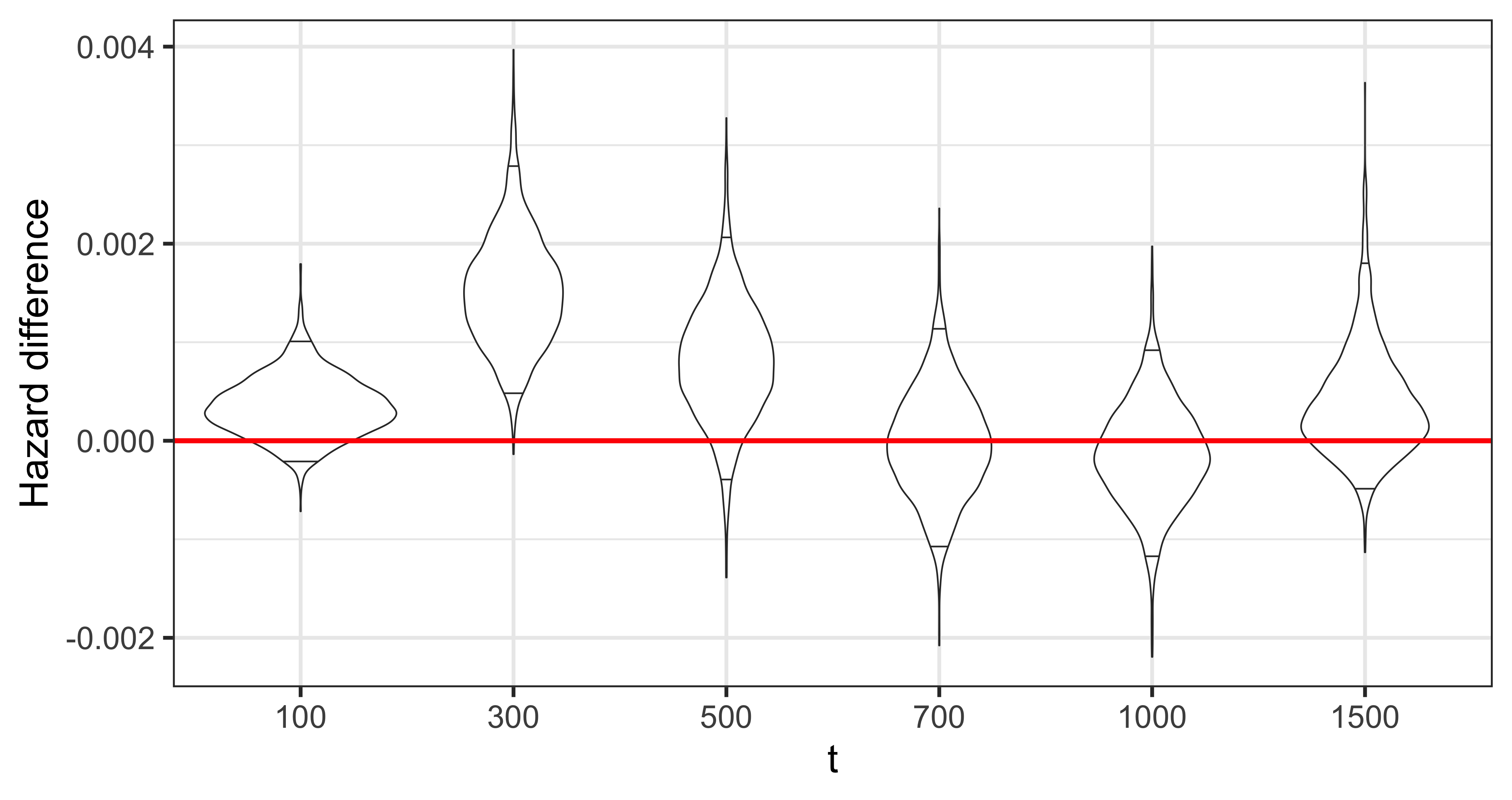
(b) $h_{B}(t)-h_{A}(t)$

Figure 10: Small cell lung cancer data. Panels (a) and (b) show, through violin plots, the posterior distributions of the difference between the two treatment survival and hazard functions at six specific time points, $t=$ 100, 300, 500, 700, 1000, and 1500 days. The short black solid lines within each violin plot indicate the 95% posterior credible interval.

The DDP-based Erlang mixture model is applied with $x\in{\cal X}=\{A,B\}$. The priors are set as follows: $\alpha\sim\text{Ga}(5,1)$; $\theta_{x}\overset{ind.}{\sim}\text{Ga}(2,50)$; $M_{x}\mid\theta_{x}\overset{ind.}{\sim}$ $\text{Unif}\left(\left\lceil 2500/\theta_{x}\right\rceil,\dots,\left\lceil 10000/\theta_{x}\right\rceil\right)$; $\bm{\mu}\sim\text{N}_{2}((6.7,6.3)^{\prime},10\,\mbox{I}_{2})$; and, $\Sigma=3\,\mbox{I}_{2}$. Here, $(6.7,6.3)^{\prime}$ are the averages of the observed survival times for each treatment after logarithmic transformation.

Posterior mean and interval estimates for the density, survival, and hazard function are compared across the two treatments in Figure 9. The Arm B density estimate is more peaked, and the mode under Arm B is estimated to be smaller than that under Arm A. The posterior mean estimates for the survival functions indicate that survival time under Arm B is stochastically smaller than that under Arm A. However, we note the overlap in the interval estimates for the two treatment survival functions for smaller time points and, more emphatically, for time points beyond about $t=700$ days. Based on the hazard function posterior mean estimates, the hazard rate under arm B is larger than that under arm A, with the exception of the time interval from about 700 to 1100 days that corresponds to a crossing of the estimated hazard functions. In this case, there is even more substantial overlap of the interval estimates, driven by the large posterior uncertainty for the arm B hazard rate estimate. Nonetheless, the estimates strongly suggest that the proportional hazards assumption is not suitable for this study.

For a more focused comparison of the two treatments, Figure 10 plots the entire posterior distribution for the difference between the survival and hazard functions at six specific time points, $t=$ 100, 300, 500, 700, 1000, and 1500 days. The lines within each violin plot indicate the 95% posterior credible interval for $S_{B}(t)-S_{A}(t)$ and $h_{B}(t)-h_{A}(t)$, and can thus be contrasted with the horizontal reference line at $0$. Based on the 95% interval estimate, treatment A outperforms treatment B at $t=$ 300, 500 and 700 days with respect to survival probability, and at $t=$ 300 days according to hazard rate.

5 Summary

We have developed a parsimonious Erlang mixture model as a general methodological tool for nonparametric Bayesian survival analysis. The model is built from a basis representation for the survival density, using Erlang basis densities with a common scale parameter. The weights are defined through increments of a random distribution function, which is flexibly modeled with a Dirichlet process prior. Utilizing a common-weights dependent Dirichlet process prior, the model has been extended to accommodate a categorical covariate associated with a generic control-treatment setting. The proposed methodology provides a useful balance between model flexibility and computational efficiency. The models were illustrated with synthetic and real data examples.

Appendix A: MCMC algorithm for the DP-based Erlang mixture model

In this section, we provide details of posterior simulation for the DP-based Erlang mixture model in Section 2.1. Recall that we have the augmented model using latent variables $\phi_{i}$,

$$t_{i}\mid\phi_{i},\theta,M \overset{ind.}{\sim} \sum_{m=1}^{M}\mathbbm{1}_{B_{m}}(\phi_{i})\text{Ga}(t\mid m,\theta),$$

$$(\phi_{1},\dots,\phi_{n})\mid\alpha,\zeta \sim \text{Exp}(\phi_{1}\mid\zeta)\prod_{i=2}^{n}\left\{\frac{\alpha}{\alpha+i-1}\text{Exp}(\phi_{i}\mid\zeta)+\frac{1}{\alpha+i-1}\sum_{j=1}^{i-1}\delta_{\phi_{j}}(\phi_{i})\right\},$$

$$\zeta \sim \text{inv-Ga}(a_{\zeta},b_{\zeta}),$$

$$\theta \sim \text{Ga}(a_{\theta},b_{\theta}),$$

$$M\mid\theta \sim \text{Unif}(\left\lceil M_{1}/\theta\right\rceil,\dots,\left\lceil M_{2}/\theta\right\rceil),$$

$$\alpha \sim \text{Ga}(a_{\alpha},b_{\alpha}),$$

where $B_{m}=((m-1)\theta,m\theta]$ for $m=1,\dots,M-1$, and $B_{M}=((M-1)\theta,\infty)$. Here, $\text{Ga}(t\mid a,b)$ denotes the density of the gamma distribution with shape parameter $a$ and scale parameter $b$ evaluated at $t$, and $\text{Exp}(\phi\mid a)$ the density of the exponential distribution with mean parameter $a$ evaluated at $\phi$. The likelihood function under the augmented model can be written as

$$L(M,\theta,\bm{\phi};\mathcal{D})=\prod_{i=1}^{n}\sum_{m=1}^{M}\left\{\mathbbm{1}_{B_{m}}(\phi_{i})\text{Ga}(y_{i}\mid m,\theta)\right\}^{\nu_{i}}\left\{\mathbbm{1}_{B_{m}}(\phi_{i})S_{\text{Ga}}(y_{i}\mid m,\theta)\right\}^{1-\nu_{i}},$$ (8)

where $S_{\text{Ga}}(y_{i}\mid m,\theta)=\int_{y_{i}}^{\infty}\text{Ga}(u\mid m,\theta)du$, $\bm{\phi}=(\phi_{1},\ldots,\phi_{n})$, and ${\cal D}=\{(y_{i},\nu_{i}),i=1,\ldots,n\}$. The joint posterior distribution of the random parameters, $\bm{\phi},\theta,M,\zeta$, and $\alpha$ is

$$p(\bm{\phi},\theta,M,\zeta,\alpha\mid\mathcal{D}) \propto \prod_{i=1}^{n}\sum_{m=1}^{M}\left\{\mathbbm{1}_{B_{m}}(\phi_{i})\text{Ga}(y_{i}\mid m,\theta)\right\}^{\nu_{i}}\left\{\mathbbm{1}_{B_{m}}(\phi_{i})S_{\text{Ga}}(y_{i}\mid m,\theta)\right\}^{1-\nu_{i}}$$

$$~{}~{}~{}~{}\times p(\bm{\phi}\mid\alpha,\zeta)p(\zeta)p(\theta)p(M\mid\theta)p(\alpha).$$

We use a Metropolis-within-Gibbs algorithm for posterior simulation if direct sampling is not available. The parameters in the proposal distributions for Metropolis-Hastings update are automatically tuned by adaptive Metropolis-Hastings algorithms in Roberts & Rosenthal (2009) for fast convergence and improved mixing. We checked mixing and convergence of the Markov chain and did not find any evidence of converging to a wrong distribution. The full conditionals are given below.

1. $M$ and $\theta$

   • Sample $M$ from the following categorical distribution,

     $$p(M=j_{M}\mid-)=\frac{L(M=j_{M},\theta,\bm{\phi};\mathcal{D})}{\sum_{i_{M}=\left\lceil\frac{M_{1}}{\theta}\right\rceil}^{\left\lceil\frac{M_{2}}{\theta}\right\rceil}L(M=i_{M},\theta,\bm{\phi};\mathcal{D})},\ ~{}~{}~{}~{}j_{M}=\left\lceil\frac{M_{1}}{\theta}\right\rceil,\ldots,\left\lceil\frac{M_{2}}{\theta}\right\rceil,$$

     where $L(j_{M},\theta,\bm{\phi};\mathcal{D})$ is the likelihood function of the augmented model in (8) evaluated with $M=j_{M}$ and the current values of $\bm{\phi}$ and $\theta$.

   • The full conditional of $\theta$ is

     $$p(\theta\mid-)\propto\text{Ga}(\theta\mid a_{\theta},b_{\theta})L(M,\theta,\bm{\phi};\cal D).$$

     We update $\theta$ using a random walk Metropolis-Hasting algorithm.

   • We also jointly update $(M,\theta)$ via a Metropolis-Hasting algorithm. Given the current values $(M^{(t-1)},\theta^{(t-1)})$ at iteration $t$, we first generate a proposal, $\theta^{\star}$ of $\theta$; $\log(\theta^{*})\sim\text{N}(\log(\theta^{(t-1)}),\epsilon)$, where $\epsilon$ is an adaptive step size, and generate $M^{\star}$ from

     $$q(M^{\star}=j_{M}\mid M^{(t-1)},\theta^{\star})=\frac{\{(j_{M}-M^{(t-1)})^{2}+1\}^{-1}}{\sum_{i_{M}=\left\lceil\frac{M_{1}}{\theta}\right\rceil}^{\left\lceil\frac{M_{2}}{\theta}\right\rceil}\{(i_{M}-M^{(t-1)})^{2}+1\}^{-1}},~{}~{}~{}j_{M}=\left\lceil\frac{M_{1}}{\theta^{*}}\right\rceil,\dots,\left\lceil\frac{M_{2}}{\theta^{*}}\right\rceil.$$

     We then accept $(\theta^{\star},M^{\star})$ with probability $\min(1,r^{\star})$, where

     $$r^{\star}=\frac{\theta^{\star}p(\theta^{\star})p(M^{\star}\mid\theta^{\star})L(M^{\star},\theta^{\star},\bm{\phi};\mathcal{D})q(M^{(t-1)}\mid\theta^{(t-1)},M^{\star})}{\theta^{(t-1)}p(\theta^{(t-1)})p(M^{(t-1)}\mid\theta^{(t-1)})L(M^{(t-1)},\theta^{(t-1)},\bm{\phi};\mathcal{D})q(M^{\star}\mid\theta^{\star},M^{(t-1)})}.$$

2. $\zeta$
   Let $\bm{\phi^{\star}}=(\phi_{1}^{\star},\dots,\phi^{\star}_{n^{\star}})$ the set of all distinct values in $(\phi_{1},\dots,\phi_{n})$ and $n^{\star}$ the number of elements in $\bm{\phi^{\star}}$. The full conditional of $\zeta$ is

   $$\text{inv-Ga}\left(a_{\zeta}+n^{\star},b_{\zeta}+\sum_{j=1}^{n^{\star}}\phi_{j}^{\star}\right).$$

3. $\alpha$
   We use the augmentation method in (Escobar & West, 1995) to update $\alpha$. We first introduce an auxiliary variable $\eta$, $\eta\mid\alpha,n\sim\text{Be}(\alpha+1,n)$, and sample $\alpha$ from a mixture of two gamma distributions;

   $$\alpha\mid- \sim \frac{a_{\alpha}+n^{\star}-1}{n(b_{\alpha}^{-1}-\log(\eta))+a_{\alpha}+n^{\star}-1}\text{Ga}(a_{\alpha}+n^{\star},(b_{\alpha}^{-1}-\log(\eta))^{-1})$$

   $$~{}~{}~{}~{}+\frac{n(b_{\alpha}^{-1}-\log(\eta))}{n(b_{\alpha}^{-1}-\log(\eta))+a_{\alpha}+n^{\star}-1}\text{Ga}(a_{\alpha}+n^{\star}-1,(b_{\alpha}^{-1}-\log(\eta))^{-1}).$$

4. $\bm{\phi}$
   Let $\bm{\phi}_{i}^{\star-}=(\phi_{1}^{\star-},\dots,\phi_{n^{\star-}}^{\star-})$ be the set of distinct values in $\bm{\phi}_{-i}$, where $\bm{\phi}_{-i}=(\phi_{1},\dots,\phi_{i-1},$ $\phi_{i+1},\dots,\phi_{n})$ and $n^{\star-}$ is the number of elements in $\bm{\phi}_{i}^{\star-}$. Let $n_{j}^{-}$ be the number of elements in $\bm{\phi}_{-i}$ that equal $\phi_{j}^{\star-}$. The full conditional of $\phi_{i}$ is

   $$\phi_{i}\mid\bm{\phi}_{-i},y_{i},\alpha,\zeta,\theta,M \sim \frac{\alpha q_{0}}{\alpha q_{0}+\sum^{n^{*-}}_{j=1}n^{-}_{j}q_{j}}h(\phi_{i}\mid y_{i},\theta,M,\zeta)$$

   $$~{}~{}~{}~{}~{}~{}+\sum^{n^{\star-}}_{j=1}\frac{n_{j}^{-}q_{j}}{\alpha q_{0}+\sum_{k=1}^{n^{\star-}}n^{-}_{k}q_{k}}\delta_{\phi_{j}^{*-}}(\phi_{i}),$$

   where

   $$q_{0} = \sum^{M-1}_{m=1}\left\{G_{\text{Exp}}(m\theta\mid\zeta)-G_{\text{Exp}}((m-1)\theta\mid\zeta)\right\}\{\text{Ga}(y_{i}\mid m,\theta)\}^{\nu_{i}}\{S_{\text{Ga}}(y_{i}\mid m,\theta)\}^{1-\nu_{i}}$$

   $$~{}~{}~{}~{}~{}+\left\{1-G_{\text{Exp}}((M-1)\theta\mid\zeta)\right\}\{\text{Ga}(y_{i}\mid m,\theta)\}^{\nu_{i}}\{S_{\text{Ga}}(y_{i}\mid m,\theta)\}^{1-\nu_{i}},$$

   $$q_{j} = \sum^{M-1}_{m=1}\mathbbm{1}_{((m-1)\theta,m\theta]}(\phi_{j}^{*-})\{\text{Ga}(y_{i}\mid m,\theta)\}^{\nu_{i}}\{S_{\text{Ga}}(y_{i}\mid m,\theta)\}^{1-\nu_{i}}$$

   $$~{}~{}~{}~{}~{}+\mathbbm{1}_{((M-1)\theta,\infty)}(\phi_{j}^{*-})\{\text{Ga}(y_{i}\mid m,\theta)\}^{\nu_{i}}\{S_{\text{Ga}}(y_{i}\mid m,\theta)\}^{1-\nu_{i}},$$

   with $G_{\text{Exp}}(\cdot\mid\zeta)$ denoting the exponential distribution function with mean $\zeta$, and

   $$h(\phi_{i}\mid y_{i},\theta,M,\zeta) = \sum_{m=1}^{M}\Omega_{m}\text{T-Exp}_{m}(\phi_{i}\mid\zeta),$$

   with

   $$\Omega_{m} = \{\text{Ga}(y_{i}\mid m,\theta)\}^{\nu_{i}}\{S_{\text{Ga}}(y_{i}\mid m,\theta)\}^{1-\nu_{i}}$$

   $$\times(G_{\text{Exp}}(m\theta\mid\zeta)-G_{\text{Exp}}((m-1)\theta\mid\zeta))q_{0}^{-1},m=1,\ldots,M-1,$$

   $$\Omega_{M} = \{\text{Ga}(y_{i}\mid M,\theta)\}^{\nu_{i}}\{S_{\text{Ga}}(y_{i}\mid M,\theta)\}^{1-\nu_{i}}$$

   $$\times(1-G_{\text{Exp}}((M-1)\theta\mid\zeta))q_{0}^{-1}.$$

   Here, $h(\phi_{i}\mid y_{i},\theta,M,\zeta)$ is a mixture of truncated exponential distributions, and $\text{T-Exp}_{m}(\phi\mid\zeta)$ is the density function of the truncated exponential distribution with mean parameter $\zeta$ with the support $((m-1)\theta,m\theta]$. $\phi_{i}$ is equal to $\phi_{j}^{\star-}$ with probability $n_{j}^{-}q_{j}/A$, where $A=\alpha q_{0}+\sum_{h=1}^{n^{\star-}}n^{-}_{h}q_{h}$; or it is drawn from $h(\phi_{i}\mid t_{i},\theta,M,\zeta)$. The inverse-cdf sampling method can be used to draw a sample from $h(\phi_{i}\mid t_{i},\theta,M,\zeta)$.

Appendix B: MCMC algorithm for the DDP mixture model

We present here the posterior simulation details for the model developed in Section 2.2. The augmented model using latent variables $\bm{\varphi}_{i}=(\varphi_{Ci},\varphi_{Ti})$ is written as

$$t_{i}\mid M_{x_{i}},\theta_{x_{i}},\varphi_{x_{i}} \overset{ind.}{\sim} \sum_{m=1}^{M_{x_{i}}}\mathbbm{1}_{B_{x_{i}m}}(\varphi_{x_{i},i})\text{Ga}(t\mid m,\theta_{x_{i}}),~{}i=1,\ldots,n,\mbox{ and }x_{i}\in\{C,T\},$$

$$(\bm{\varphi}_{1},\dots,\bm{\varphi}_{n})\mid\alpha,\bm{\mu} \sim \text{LN}_{2}(\bm{\varphi}_{1}\mid\bm{\mu},\Sigma)\prod_{i=2}^{n}\left\{\frac{\alpha}{\alpha+i-1}\text{LN}_{2}(\bm{\varphi}_{i}\mid\bm{\mu},\Sigma)+\frac{1}{\alpha+i-1}\sum_{j=1}^{i-1}\delta_{\bm{\varphi}_{j}}(\bm{\varphi}_{i})\right\},$$

$$\theta_{x} \overset{ind.}{\sim} \text{Ga}(a_{x\theta},b_{x\theta}),$$

$$M_{x}\mid\theta_{x} \overset{ind.}{\sim} \text{Unif}(\left\lceil M_{x1}/\theta_{x}\right\rceil,\dots,\left\lceil M_{x2}/\theta_{x}\right\rceil),$$

$$\alpha \sim \text{Ga}(a_{\alpha},b_{\alpha}),$$

$$\bm{\mu} \sim \text{N}_{2}(\bar{\bm{\mu}},\Sigma_{0}),$$

where $B_{x_{i}m}=((m-1)\theta_{x_{i}},m\theta_{x_{i}}]$ for $m=1,\dots,M_{x_{i}}-1$, and $B_{x_{i}M_{x_{i}}}=((M_{x_{i}}-1)\theta_{x_{i}},\infty)$. The likelihood function for the augmented model for observation $i$ is

$$L_{i}(M_{x_{i}},\theta_{x_{i}},\varphi_{x_{i},i};\mathcal{D})=\left[\sum_{m=1}^{M_{x_{i}}}\mathbbm{1}_{B_{x_{i}m}}(\varphi_{x_{i},i})\text{Ga}(y_{i}\mid m,\theta_{x_{i}})\right]^{\nu_{i}}\left[\sum_{m=1}^{M_{x_{i}}}\mathbbm{1}_{B_{x_{i}m}}(\varphi_{x_{i},i})S_{\text{Ga}}(y_{i}\mid m,\theta_{x_{i}})\right]^{1-\nu_{i}}.$$

where $\cal D=\{(y_{i},\nu_{i},x_{i}),i=1,\ldots,n\}$ denotes data. Similar to the algorithm in Appendix A, we use an adaptive Metropolis-within-Gibbs algorithm in Roberts & Rosenthal (2009) for the Metropolis-Hastings updates. Mixing and convergence of Markov chain are checked and no evidence is found of converging to a wrong distribution. The full conditionals are given below.

1. $\bm{M}=(M_{C},M_{T})$
   Sample $M_{C}$ from the following categorical distribution,

   $$p(M_{C}=j_{M}\mid-)=\frac{L_{C}(j_{M},\theta_{C},\bm{\varphi};\mathcal{D})}{\sum_{i_{M}=\left\lceil\frac{M_{C1}}{\theta_{C}}\right\rceil}^{\left\lceil\frac{M_{C2}}{\theta_{C}}\right\rceil}L_{C}(i_{M},\theta_{C},\bm{\varphi};\mathcal{D})},\ ~{}~{}~{}~{}j_{M}=\left\lceil\frac{M_{C1}}{\theta_{C}}\right\rceil,\ldots,\left\lceil\frac{M_{C2}}{\theta_{C}}\right\rceil,$$

   where $L_{C}(j_{M},\theta_{C},\bm{\varphi};\mathcal{D})=\prod_{i:x_{i}=C}L_{i}(j_{M},\theta_{C},\varphi_{Ci};\mathcal{D})$. We then draw $M_{T}$ in a similar way.

2. $\bm{\theta}=(\theta_{C},\theta_{T})$
   The full conditional of $\bm{\theta}$ is

   $$p(\bm{\theta}\mid-)\propto\text{Ga}(\theta_{C}\mid a_{C\theta},b_{C\theta})\text{Ga}(\theta_{T}\mid a_{T\theta},b_{T\theta})\prod_{i=1}^{n}L_{i}(M_{x_{i}},\theta_{x_{i}},\varphi_{x_{i},i};\cal{D}).$$

   We use the algorithm in Roberts & Rosenthal (2009) to sample $\bm{\theta}$. Let $\bm{\theta}^{(t-1})=(\theta^{(t-1}_{C},\theta^{(t01})_{T})$ the current values of $\bm{\theta}$. A proposal of $\bm{\theta}$ is generated from

   $$\begin{split}\log(\bm{\theta}^{\star})\sim&0.95\text{N}(\log(\bm{\theta}^{(t-1)}),2.38^{2}/2\Sigma_{n})+0.05\text{N}(\log(\bm{\theta}^{(t-1)}),0.01/2I_{2}),\end{split}$$

   where $\Sigma_{n}$ is the empirical covariance matrix of $\log(\bm{\theta})$ based on the run so far. Then we accept $\bm{\theta}^{\star}$ with probability $\min(1,r^{\star})$, where

   $$r^{\star}=\frac{\theta_{C}^{\star}\theta_{T}^{\star}\text{Ga}(\theta_{C}^{\star}|a_{C\theta},b_{C\theta})\text{Ga}(\theta_{T}^{\star}\mid a_{T\theta},b_{T\theta})\prod_{i=1}^{n}L_{i}(M_{x_{i}},\theta_{x_{i}}^{\star},\varphi_{x_{i},i};\cal{D})}{\theta_{C}^{(t-1)}\theta_{T}^{(t-1)}\text{Ga}(\theta_{C}^{(t-1)}\mid a_{C\theta},b_{C\theta})\text{Ga}(\theta_{T}^{(t-1)}\mid a_{T\theta},b_{T\theta})\prod_{i=1}^{n}L_{i}(M_{x_{i}},\theta_{x_{i}}^{(t-1)},\varphi_{x_{i},i};\cal{D})}.$$

3. $\bm{\mu}$
   Let $\bm{\varphi}^{\star}=(\bm{\varphi}_{1}^{\star},\dots,\bm{\varphi}_{n^{\star}}^{\star})$ be the set of distinct values in $\bm{\varphi}$, where $n^{\star}$ is the number of elements in $\bm{\varphi}^{\star}$. The full conditional of $\bm{\mu}$ is

   $$\text{N}_{2}(\bm{\mu}_{1},\Sigma_{1}),$$

   where

   $$\Sigma_{1}=\left[\Sigma_{0}^{-1}+{n^{\star}}\Sigma^{-1}\right]^{-1}~{}~{}\text{ and }~{}~{}\bm{\mu}_{1}=\Sigma_{1}\left[\Sigma_{0}^{-1}\bm{\bar{\mu}}+\Sigma^{-1}\sum_{i=1}^{n^{\star}}\log(\bm{\varphi}_{i}^{\star})\right].$$

4. $\alpha$
   We use the augmentation method in Escobar & West (1995) to update $\alpha$. We first introduce an auxiliary variable $\eta$, $\eta\mid\alpha,n\sim\text{Be}(\alpha+1,n)$, and sample $\alpha$ from a mixture of two gamma distributions;

   $$\alpha\mid- \sim \frac{a_{\alpha}+n^{\star}-1}{n(b_{\alpha}^{-1}-\log(\eta))+a_{\alpha}+n^{\star}-1}\text{Ga}(a_{\alpha}+n^{\star},(b_{\alpha}^{-1}-\log(\eta))^{-1})$$

   $$~{}~{}~{}~{}+\frac{n(b_{\alpha}^{-1}-\log(\eta))}{n(b_{\alpha}^{-1}-\log(\eta))+a_{\alpha}+n^{\star}-1}\text{Ga}(a_{\alpha}+n^{\star}-1,(b_{\alpha}^{-1}-\log(\eta))^{-1}).$$

5. $\bm{\varphi}$
   Let $\bm{\varphi}_{i}^{\star-}=(\bm{\varphi}_{1}^{\star-},\dots,\bm{\varphi}_{n^{\star-}}^{\star-})$ be the set of distinct values in $\bm{\varphi}_{-i}=$ $(\bm{\varphi}_{1},\dots,\bm{\varphi}_{i-1},$ $\bm{\varphi}_{i+1},\dots,\bm{\varphi}_{n})$, where $n^{\star-}$ is the number of elements in $\bm{\varphi}_{i}^{\star-}$. Let $n_{j}^{-}$ be number of elements in $\bm{\varphi_{-i}}$ that is equal to $\bm{\varphi}_{j}^{\star-}$. The full conditional of $\bm{\varphi}_{i}$ is

   $$\bm{\varphi}_{i}\mid\bm{\varphi}_{-i},\bm{\mu},\Sigma,\bm{\theta},\bm{M},\mathcal{D} \sim \frac{\alpha q_{0}}{\alpha q_{0}+\sum_{j=1}^{n^{*-}}n_{j}^{-}q_{j}}h(\bm{\varphi}_{i}\mid y_{i},\bm{\mu},\Sigma,\bm{\theta},\bm{M})$$

   $$~{}~{}~{}~{}~{}~{}~{}+\sum_{j=1}^{n^{\star-}}\frac{n_{j}^{-}q_{j}}{\alpha q_{0}+\sum_{j=1}^{n^{*-}}n_{j}^{-}q_{j}}\delta_{\bm{\varphi}^{*-}_{j}}(\bm{\varphi}_{i}),$$

   where, for $x_{i}=C$,

   $$q_{0} = \sum_{m=1}^{M_{C}-1}\{\text{Ga}(y_{i}\mid m,\theta_{C})\}^{\nu_{i}}\{S_{\text{Ga}}(y_{i}\mid m,\theta_{C})\}^{1-\nu_{i}}$$

   $$~{}~{}~{}~{}\times\{G_{\text{LN}}(m\theta_{C}\mid\mu_{C\mid T},\Sigma_{C\mid T})-(G_{\text{LN}}((m-1)\theta_{C}\mid\mu_{C\mid T},\Sigma_{C\mid T})\}$$

   $$~{}~{}~{}~{}~{}+\{\text{Ga}(y_{i}\mid M_{C},\theta_{C})\}^{\nu_{i}}\{S_{\text{Ga}}(y_{i}\mid M_{C},\theta_{C})\}^{1-\nu_{i}}\{1-G_{\text{LN}}((M_{C}-1)\theta_{C}\mid\mu_{C\mid T},\Sigma_{C\mid T})\},$$

   $$q_{j} = \sum_{m=1}^{M_{C}-1}\mathbbm{1}_{((m-1)\theta_{C},m\theta_{C}]}(\varphi_{Ci}^{\star-})\{\text{Ga}(y_{i}|m,\theta_{C})\}^{\nu_{i}}\{S_{\text{Ga}}(y_{i}|m,\theta_{C})\}^{1-\nu_{i}}$$

   $$~{}~{}~{}~{}+\mathbbm{1}_{((M_{C}-1)\theta_{C},\infty)}(\varphi_{Ci}^{\star-})\{\text{Ga}(y_{i}|M_{C},\theta_{C})\}^{\nu_{i}}\{S_{\text{Ga}}(y_{i}|M_{C},\theta_{C})\}^{1-\nu_{i}},$$

   $$\mu_{C\mid T} = \mu_{1}+\Sigma_{12}/\Sigma_{22}(\varphi_{Ti}-\mu_{2}),$$

   $$\Sigma_{C\mid T} = \Sigma_{11}-\Sigma_{12}\Sigma_{21}/\Sigma_{22}$$

   with $G_{\text{LN}}(\cdot\mid\mu_{C\mid T},\Sigma_{C\mid T})$ denoting a lognormal distribution function with mean $\mu_{C\mid T}$ and variance $\Sigma_{C\mid T}$, and

   $$h(\bm{\varphi}_{i}\mid y_{i},\bm{\mu},\Sigma,\bm{\theta},\bm{M}) = \text{LN}(\varphi_{Ti}\mid\mu_{1},\Sigma_{11})\times\sum_{m=1}^{M_{C}}\Omega_{m}\text{T-LN}_{m}(\varphi_{Ci}\mid\mu_{C\mid T},\Sigma_{C\mid T})$$

   with

   $$\Omega_{m} = \{\text{Ga}(y_{i}\mid m,\theta_{C})\}^{\nu_{i}}\{S_{\text{Ga}}(y_{i}\mid m,\theta_{C})\}^{1-\nu_{i}}$$

   $$~{}~{}~{}~{}~{}\times\{G_{\text{LN}}(m\theta_{C}\mid\mu_{C\mid T},\Sigma_{C\mid T})-G_{\text{LN}}((m-1)\theta_{C}\mid\mu_{C\mid T},\Sigma_{C\mid T})\}q_{0}^{-1},$$

   $$\hskip 72.26999pt\mbox{ for }m=1,\dots,M_{C}-1,$$

   $$\Omega_{M_{C}} = \{\text{Ga}(y_{i}\mid M_{C},\theta_{C})\}^{\nu_{i}}\{S_{\text{Ga}}(y_{i}\mid M_{C},\theta_{C})\}^{1-\nu_{i}}$$

   $$~{}~{}~{}~{}~{}\times\{1-G_{\text{LN}}((M_{C}-1)\theta_{C}\mid\mu_{C\mid T},\Sigma_{C\mid T})\}q_{0}^{-1}.$$

   Similar to the algorithm of updating $\varphi_{i}$ for the DP-based Erlang mixture model, we let $\bm{\varphi}_{i}=\bm{\varphi}_{j}^{\star-}$ with probability $n_{j}^{-}q_{j}/A$, where $A=\alpha q_{0}+\sum_{h=1}^{n^{\star-}}n_{h}^{-}q_{h}$, or draw a new $\bm{\varphi}_{i}$ from $h(\bm{\varphi}_{i}\mid y_{i},\bm{\mu},\Sigma,\bm{\theta},\bm{M})$ with probability $\alpha q_{0}/A$. To draw a sample from $h(\bm{\varphi}_{i}\mid y_{i},\bm{\mu},\Sigma,\bm{\theta},\bm{M})$, we first draw $\varphi_{Ti}$ from $\text{LN}(\mu_{1},\Sigma_{11})$ and then, conditional on $\varphi_{Ti}$, draw $\varphi_{Ci}$ from a mixture of truncated lognormal distributions using an inverse-cdf sampling method, where each component, $\text{T-LN}_{m}$ is a lognormal distribution with support of $((m-1)\theta_{C},m\theta_{C}]$. The same method is applied for the observations with $x_{i}=T$ by simply switching $C$ with $T$.

References

- (1)
- Antoniadis et al. (1999) Antoniadis, A., Grégoire, G. & Nason, G. (1999), ‘Density and hazard rate estimation for right-censored data by using wavelet methods’, Journal of the Royal Statistical Society: Series B (Methodological) 61, 63–84.
- Blackwell & MacQueen (1973) Blackwell, D. & MacQueen, J. B. (1973), ‘Ferguson distributions via Pólya urn schemes’, Annals of Statistics 1, 353–355.
- Butzer (1954) Butzer, P. (1954), ‘On the extensions of Bernstein polynomials to the infinite interval’, Proceedings of the American Mathematical Society 5, 547–553.
- De Iorio et al. (2009) De Iorio, M., Johnson, W. O., Müller, P. & Rosner, G. L. (2009), ‘Bayesian nonparametric nonproportional hazards survival modeling’, Biometrics 65, 762–771.
- Escobar & West (1995) Escobar, M. D. & West, M. (1995), ‘Bayesian density estimation and inference using mixtures’, Journal of the American Statistical Association 90, 577–588.
- Ferguson (1973) Ferguson, T. S. (1973), ‘A Bayesian analysis of some nonparametric problems’, The Annals of Statistics 1, 209–230.
- Hanson (2006) Hanson, T. E. (2006), ‘Modeling censored lifetime data using a mixture of gammas baseline’, Bayesian Analysis 1, 575–594.
- Ibrahim et al. (2001) Ibrahim, J. G., Chen, M. & Sinha, D. (2001), Bayesian Survival Analysis, Springer, New York, NY.
- Kim & Kottas (2022) Kim, H. & Kottas, A. (2022), ‘Erlang mixture modeling for Poisson process intensities’, Statistics and Computing 32, 3.
- Kottas (2006) Kottas, A. (2006), ‘Nonparametric Bayesian survival analysis using mixtures of Weibull distributions’, Journal of Statistical Planning and Inference 136, 578–596.
- Lee & Lin (2010) Lee, S. C. K. & Lin, X. S. (2010), ‘Modeling and evaluating insurance losses via mixtures of Erlang distributions’, North American Actuarial Journal 14, 107–130.
- MacEachern (2000) MacEachern, S. N. (2000), ‘Dependent Dirichlet processes’, Technical Report, Ohio State University .
- Mitra & Müller (2015) Mitra, R. & Müller, P., eds (2015), Nonparametric Bayesian Inference in Biostatistics, Springer, Cham, Switzerland.
- Müller et al. (2015) Müller, P., Quintana, F. A., Jara, A. & Hanson, T. (2015), Bayesian Nonparametric Data Analysis, Springer, Cham, Switzerland.
- Neal (2000) Neal, M. (2000), ‘Markov Chain sampling methods for Dirichlet process mixture models’, Journal of Computational and Graphical Statistics 9, 249–265.
- Phadia (2013) Phadia, E. G. (2013), Prior Processes and Their Applications, Springer, Berlin Heidelberg.
- Poynor & Kottas (2019) Poynor, V. & Kottas, A. (2019), ‘Nonparametric Bayesian inference for mean residual life functions in survival analysis.’, Biostatistics 20, 240–255.
- Quintana et al. (2022) Quintana, F. A., Müller, P., Jara, A. & MacEachern, S. N. (2022), ‘The dependent Dirichlet process and related models’, Statistical Science 37, 24–41.
- Roberts & Rosenthal (2009) Roberts, G. O. & Rosenthal, J. S. (2009), ‘Examples of adaptive MCMC’, Journal of Computational and Graphical Statistics 18, 349–367.
- Sethuraman (1994) Sethuraman, J. (1994), ‘A constructive definition of Dirichlet priors’, Statistica Sinica 4, 639–650.
- Venturini et al. (2008) Venturini, S., Dominici, F. & Parmigiani, G. (2008), ‘Gamma shape mixtures for heavy-tailed distributions’, The Annals of Applied Statistics 2, 756–776.
- Xiao et al. (2021) Xiao, S., Kottas, A., Sansó, B. & Kim, H. (2021), ‘Nonparametric Bayesian modeling and estimation for renewal processes’, Technometrics 63, 100–115.
- Ying et al. (1995) Ying, Z., Jung, S. & Wei, L. (1995), ‘Survival analysis with median regression models’, Journal of the American Statistical Association 90, 178–184.