R-Pred: Two-Stage Motion Prediction Via Tube-Query Attention-Based Trajectory Refinement

Abstract

Predicting the future motion of dynamic agents is of paramount importance to ensuring safety and assessing risks in motion planning for autonomous robots. In this study, we propose a two-stage motion prediction method, called R-Pred, designed to effectively utilize both scene and interaction context using a cascade of the initial trajectory proposal and trajectory refinement networks. The initial trajectory proposal network produces $M$ trajectory proposals corresponding to the $M$ modes of the future trajectory distribution. The trajectory refinement network enhances each of the $M$ proposals using 1) tube-query scene attention (TQSA) and 2) proposal-level interaction attention (PIA) mechanisms. TQSA uses tube-queries to aggregate local scene context features pooled from proximity around trajectory proposals of interest. PIA further enhances the trajectory proposals by modeling inter-agent interactions using a group of trajectory proposals selected by their distances from neighboring agents. Our experiments conducted on Argoverse and nuScenes datasets demonstrate that the proposed refinement network provides significant performance improvements compared to the single-stage baseline and that R-Pred achieves state-of-the-art performance in some categories of the benchmarks.

1 Introduction

In autonomous vehicles and robotics applications, dynamic objects move in complex environments while avoiding collisions with other agents. Each dynamic agent plans its motion by predicting the future motion and behavior of other agents around it. Motion prediction refers to the task of predicting the future trajectory of dynamic agents based on their past trajectory history and information on the surrounding environment. The task of predicting motion is challenging because the trajectory of an agent is affected by a variety of contextual factors, which must be taken into account when modeling motion. In the context of autonomous vehicles, examples of such factors include permissible roads, lanes, traffic signals, blinker states, interactions with other agents, and so forth. The difficulty of predicting future motion also arises from the fact that the distribution of future trajectories tends to be multi-modal. In a given scene, a target agent can choose one of several distinct maneuvers such as changing lanes, turning left, turning right, or continuing straight ahead. Accordingly, prediction models should be able to generate one or more plausible future trajectories with probabilities.

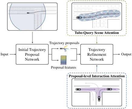
Figure 1: Key concept of R-Pred. R-Pred performs two stages of trajectory prediction. ITPNet produces $M$ trajectory proposals with the corresponding proposal features and TRNet refines each trajectory proposal using separate networks. ITPNet uses a scene context acquired from a relatively large area, whereas TRNet uses a local scene context that exists in a tube-shaped area. TRNet also refines the trajectory proposal using an inter-agent interaction context represented at a proposal level.

Recently, deep neural networks have been developed as a new paradigm in trajectory prediction, and have achieved considerable improvements in performance compared to traditional prediction models through data-driven modeling of trajectory data. Sequence modeling networks such as long short term memory (LSTM) [23] or gated recurrent unit (GRU) [6] architectures have been shown to be effective in representing sequential trajectory data [25, 26]. Trajectory prediction task has been successfully performed using encoder-decoder architectures [35, 53, 29, 30, 16, 19, 45, 55, 43, 32, 26, 15, 17, 10, 8, 20, 24, 40, 28, 36]. Recently, the accuracy of trajectory prediction has been rapidly improved by utilizing various sources of contextual information available for prediction. Numerous methods have jointly modeled the trajectories of multiple neighboring agents to account for their interactions, including social-LSTM [1], soft hardwired attention [12], social GAN [20], MATF [54], Trajectron [24, 40], DESIRE [28], DATF [36], and SoPhie [39]. Static scene information around the target agent was also used to generate more physically plausible trajectories. A scene was represented by a two-dimensional raster image that describes the scene [11, 4, 7, 32, 37, 52]. A vector representation of the scene was also proposed for scene encoding [13, 29, 53, 19, 55, 26, 16, 34, 30, 10, 45, 47, 48]. Recently, Transformer models [44] have been used to model the scene and interaction context using the attention mechanism [30, 34, 55, 33, 45, 50].

In this paper, we propose a new two-stage motion prediction framework, referred to as R-Pred. As shown in Fig. 1, the proposed R-Pred architecture consists of two-stage networks: an initial trajectory proposal network (ITPNet) and a trajectory refinement network (TRNet). The ITPNet produces $M$ initial trajectory proposals corresponding to the $M$ modes of the trajectory distribution for a target agent. TRNet then refines each trajectory proposal using the contexts customized for each proposal. Using the initial trajectory proposals as a priori information, TRNet can utilize the scene and interaction contexts in more selective and effective ways.

TRNet employs the following two refinement sub-modules. First, we present tube-query scene attention (TQSA) to utilize the local scene context effectively. Unlike ITPNet, which uses a global scene context, TQSA extracts local scene context features within a tube-shaped region around each trajectory proposal. (See Fig. 1 for illustration). Then, the extracted scene context features are used to enhance the corresponding trajectory proposal through cross-attention mechanism. TQSA allows the important scene context to be used to improve each $M$ trajectory proposal. Second, we propose the proposal-level interaction attention (PIA) mechanism. PIA models inter-agent interactions using the trajectory proposals produced for multiple neighboring agents by ITPNet. PIA selects a group of trajectory proposals that have the highest influence on the trajectory proposal of interest using the distance-wise proposal grouping strategy. The proposal group is used to refine the trajectory of interest through cross-attention.

In fact, our per-proposal refinement strategy is motivated by two-stage object detectors (e.g., Faster RCNN [38]), where the initial object proposals are first obtained from the entire convolutional neural network (CNN) features and then local features in the region of interest (RoI) are pooled to refine each object proposal [18, 38, 21]. Similarly, R-Pred generates the context features based on the initial trajectory proposals produced by ITPNet and uses them to refine each proposal.

By combining these two sub-modules, R-Pred can generate refined trajectory outputs. We conducted an experimental evaluation of the proposed approach on the generally used Argoverse [5] and nuScenes [3] datasets, and the results demonstrate that the proposed refinement network significantly improved the accuracy of ITPNet baseline. The results also show that R-Pred achieves the state-of-the-art performance in some categories of official Argoverse and nuScenes leaderboards.

The main contributions are summarized below;

• We propose a novel trajectory refinement network that refines each of $M$ trajectory proposals using the local scene context and the proposal-level inter-agent interactions. The per-proposal refinement strategy effectively improves the trajectory predictions obtained by the first-stage network.

• We introduce the concept of global-to-local hierarchical attention to effectively utilize the scene context. Our refinement network uses a tube-query to gather the scene context from the local region around the proposal trajectory. The proposed global-local hierarchical attention mechanism is contrasted with factorized attention [34, 33], which iterates attention over different sources of context.

• We use trajectory proposals of neighboring agents to model interactions between agents. Using the trajectory proposal features reflecting particular intentions of other agents, PIA can better model inter-agent interactions than the conventional interaction modeling that uses the past trajectory features only.

• R-Pred can use any off-the-shelf single-stage trajectory prediction network as the initial trajectory proposal network. The proposed refinement framework can also be readily applied to any trajectory prediction network available.

• The source code used in this work will be released publicly.

2 Related Works

2.1 Context-Aware Trajectory Prediction

Numerous methods have improved the performance of trajectory prediction by leveraging the contextual information available for prediction. For example, information on the static scene around a target agent has been utilized as scene context. Raster-based scene encoding uses 2D raster images to summarize scene information and extract semantic features using convolutional neural networks [32, 4, 37, 14, 40, 9, 46]. The advantage of this approach is that different types of scene components can be easily accommodated in a raster image. However, the performance of these methods is limited owing to quantization errors and a lack of receptive fields in the encoding architectures. Vector-based scene encoding represents scene components using vectors, and encodes their relationships using a graph structure or attention models [29, 10, 40, 20, 24, 27, 13]. VectorNet [13] introduced a hierarchical graph neural network that exploited the spatial locality of road components by vectorized representation. Similarly, LaneGCN [29] was proposed as an effective graph convolutional network to represent complicated topology and long-range dependency. Trajectron++ [40] employed a directed spatio-temporal graph to represent scene context vectors while incorporating agent dynamics and heterogeneous data.

The performance of trajectory prediction has also been improved by taking into account interactions with surrounding dynamic agents and static environment information. Social pooling methods pooled the trajectory features of other agents for interaction modeling [1, 28, 20, 39, 8]. Recently, attention mechanisms have been proposed to exploit the meaningful relationships between dynamic agents and lane segments [26, 41, 55, 10, 19, 51, 29, 13, 16, 32, 45, 29].

2.2 Transformer-based Trajectory Prediction

Transformer architectures provide an efficient approach to training an attention mechanism that can capture long-distance dependencies of sequence data. Recently, Transformers have been adopted for trajectory prediction to model context in spatial and temporal domains as well as interactions between agents [50, 45, 55, 30, 33, 34]. mmTransformer [30] employed an efficient stacked Transformer that applied cross-attention on multi-agent and scene contexts one by one. HiVT [55] summarized the spatio-temporal features of agents using translation-invariant agent-centric local scene structure. In SceneTransformer [34], a simple varying form of self-attention was exploited to integrate various features, generating scene-level consistent predictions for all agents jointly. Along these lines, Wayformer [33] was proposed as a general multi-dimensional attention architecture designed to jointly encode multiple agent trajectories and map data in time, space, and agent dimensions.

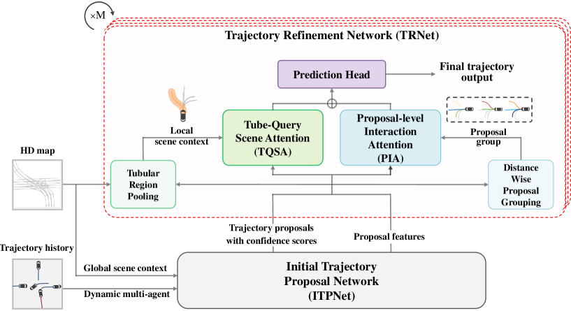
Figure 2: Overall structure of R-Pred. Given the past trajectories of the dynamic agents and the scene information, ITPNet generates $M$ trajectory proposals for each agent. TRNet refines each of the $M$ trajectory proposals of the target agent through TQSA and PIA. TQSA utilizes local scene context features obtained by tubular region pooling. PIA captures interaction context using the proposal group found by the distance-wise proposal grouping. Finally, the prediction header produces the refined future trajectories based on the joint trajectory features obtained by concatenation of the attention values from TQSA and PIA.

3 Problem Setup

Suppose that the historical trajectory states of $N$ dynamic agents are obtained from the multi-object tracker, where $N$ can vary depending on the scenario. The agent whose future trajectory is to be predicted is referred to as the target agent and the remaining agents as neighbor agents. The past trajectory states over $T$ time steps for the $i$-th agent are given by $\mathbf{x}_{i}=[x_{i}({t-T+1}),x_{i}({t-T+2}),...,x_{i}({t})]$, where $t$ denotes the current time step and $x_{i}({t-s})$ is the state of the $i$-th agent at the time step $(t-s)$. The trajectory state is of the form $(x,y,\varepsilon)$ consisting of the $(x,y)$ position and the agent’s semantic property $\varepsilon$. The $(x,y)$ coordinates are represented in the agent-centric reference frame, where the current position of a target agent is the origin and its heading angle is aligned with the positive x-axis. Similarly, the future trajectory states over $F$ time steps for the $i$-th agent are given by $\mathbf{y}_{i}=[y_{i}({t+1}),y_{i}({t+2}),...,y_{i}({t+F})]$. We assume that the vector representation of a scene is available along with the trajectory data. For instance, a lane is represented by a set of points on its centerline, where the $(x,y)$ coordinates of each point are expressed in an agent-centric frame. We accommodate different types of scene components by appending an attribute index $\epsilon_{l}$ to the $(x,y)$ coordinate as $(x,y,\epsilon_{l})$. The set of scene components around the target agent at the time $t$ is expressed as the vector $\xi=[\xi_{1},...,\xi_{L}]$, where the dimension $L$ varies depending on the scene complexity and the region of interest on the map.

Without loss of generality, let $\mathbf{x}_{1}$ be the trajectory of the target agent and $\mathbf{x}_{2},...,\mathbf{x}_{N}$ be the trajectories of neighboring agents. Finally, the goal of the motion prediction task is to estimate the future trajectory of the target agent $\mathbf{y}_{1}$ given the past trajectories of $N$ agents $\mathbf{x}_{1},...,\mathbf{x}_{N}$ and the scene information $\xi$.

4 Proposed Trajectory Prediction Network

In this section, we present the details of the proposed motion prediction method, R-Pred.

4.1 Overall Framework

An overview of the proposed R-Pred framework is presented in Fig. 2. Our proposed architecture produces $M$ multi-modal trajectory predictions for a target agent over two stages. First, ITPNet produces $M$ trajectory proposals for all $N$ agents present in the scene. Along with the trajectory proposals, ITPNet returns $M$ intermediate features used to produce the trajectory proposals. These features are called proposal features. ITPNet follows traditional trajectory prediction methods for scene and interaction encoding; that is, it utilizes the global scene context features extracted from a fixed region around the current position of the agent. In addition, the ITPNet exploits the interaction context derived from the past trajectories of $N$ agents. Second, TRNet refines each of the $M$ trajectory proposals of the target agent using the prior trajectory information generated by the ITPNet. TRNet employs TQSA and PIA to generate the context features customized for each proposal. TQSA extracts the local scene context features cropped from a tube-shaped region around the target trajectory proposal. PIA generates the inter-agent interaction context features using a group of selected proposal trajectories of $N$ agents. The context features generated by TQSA and PIA enhance the proposal features through cross-attention. The final joint trajectory features are obtained by concatenating two attention values from TQSA and PIA. Finally, the prediction head produces $M$ future trajectory predictions and their confidence scores for each target agent.

4.2 Initial Trajectory Proposal Network

Given the past trajectories $\mathbf{x}_{1},...,\mathbf{x}_{N}$ of the $N$ agents present in the scene and the scene information $\xi$, ITPNet produces $M$ trajectory proposals and their confidence scores for each agent. $M$ proposal features are also produced for the refinement step. The trajectory proposals, their confidence scores, and the proposal features for the $i$-th agent are denoted as $\hat{\mathbf{y}}_{i}=[\hat{\mathbf{y}}_{i}^{1},...,\hat{\mathbf{y}}_{i}^{M}]$, $\hat{\mathbf{c}}_{i}=[\hat{\mathbf{c}}_{i}^{1},...,\hat{\mathbf{c}}_{i}^{M}]$, and $\mathbf{f}_{i}=[\mathbf{f}_{i}^{1},...,\mathbf{f}_{i}^{M}]$, respectively.

4.3 Trajectory Refinement Network

TRNet refines the trajectory proposals $\hat{\mathbf{y}}_{1}$ of the target agent using the trajectory proposals $\hat{\mathbf{y}}_{1},...,\hat{\mathbf{y}}_{N}$, the proposal confidence scores $\hat{\mathbf{c}}_{1},...,\hat{\mathbf{c}}_{N}$, the proposal features $\mathbf{f}_{1},...,\mathbf{f}_{N}$, and the scene information $\xi$ obtained from ITPNet.

Algorithm 1 Tubular Region Pooling

0:  Trajectory proposal $\hat{\textbf{y}}_{1}^{m}$, scene context vectors $\xi$, scene embedding features $\Psi$, and thresholding radius $\tau$.

0:  Local scene context features $\Psi_{1}^{m}$.

1:  $\Psi_{1}^{m}=set()$

2:  for $f\xleftarrow{}t+1$ to $t+F$ do

3:     for each $\xi_{l}\in\xi$ do

4:        $dist=\|\hat{y}_{1}^{m}(f)-\xi_{l}\|_{2}$

5:        if $dist<\tau$ then

5:           $\Psi_{1}^{m}$.add($\psi_{l}$)

6:  

7:  return  $\Psi_{1}^{m}$

Tube-Query Scene Attention. We construct the set of scene embedding features $\Psi=\{\psi_{1},...,\psi_{L}\}$ by encoding each element of $\xi$ via a linear projection, i.e., $\psi_{l}={\rm linear\_proj}(\xi_{l})$. TQSA pools the scene embedding features in a tubular region around the trajectory proposal on the map from $\Psi$. We denote the set of scene embedding features prepared for the target trajectory proposal $\hat{\mathbf{y}}_{1}^{m}$ as $\Psi^{m}_{1}$. Tubular region pooling is efficiently performed to aggregate scene embedding features within the search radius $\tau$ around each waypoint of the trajectory proposal. Note that a collection of search disks centered at all waypoints on the trajectory forms an approximately tubular polygon. See Algorithm 1 for further details.

TQSA decodes the proposal features $\mathbf{f}_{1}^{m}$ of the target agent by performing cross-attention on the local scene context $\Psi^{m}_{1}$. Specifically, we use the proposal features $\mathbf{f}_{1}^{m}$ as the query and the local scene context features $\Psi^{m}_{1}$ as the key and value, i.e.,

$$Q=\mathbf{f}_{1}^{m}W^{Q_{TQSA}}$$ (1)

$$K=\Psi^{m}_{1}W^{K_{TQSA}}$$ (2)

$$V=\Psi^{m}_{1}W^{V_{TQSA}}$$ (3)

$$\mathcal{A}_{1}^{m}=softmax\left(\frac{QK^{\top}}{\sqrt{d_{k}}}\right)V,$$ (4)

where $W^{Q_{TQSA}}$, $W^{K_{TQSA}}$, and $W^{V_{TQSA}}$ are learnable weight matrices and $d_{k}$ is the dimension of the embedding vectors. We combine the attention value $\mathcal{A}_{1}^{m}$ and the proposal features $\mathbf{f}_{1}^{m}$ using the gating function introduced in [55]

$$\lambda=\sigma(\mathbf{f}_{1}^{m}W^{input}+\mathcal{A}_{1}^{m}W^{hidden})$$ (5)

$$\mathbf{t}_{1}^{m}=\lambda\odot\mathbf{f}_{1}^{m}W^{gate}+(1-\lambda)\odot\mathcal{A}_{1}^{m}$$ (6)

$$\mathbf{t}_{1}^{m}=\mathbf{f}_{1}^{m}+\phi(\mathbf{t}_{1}^{m}),$$ (7)

where $W^{input}$, $W^{hidden}$, and $W^{gate}$ are learnable matrices, $\odot$ indicates element-wise product, $\sigma$ indicates the sigmoid function and $\phi(\cdot)$ denotes a multi-layer perceptron (MLP). We add layer normalization [2], Dropout [42], and residual connection [22] in the middle of the attention process.

Note that the aforementioned local scene attention process to produce the output of TQSA $\textbf{t}_{1}^{m}$ is performed for each trajectory proposal (for each $m$ value) in parallel.

Method	$\textit{minADE}_{1}$	$\textit{minFDE}_{1}$	$\textit{minADE}_{6}$	$\textit{minFDE}_{6}$	$\textit{brierFDE}_{6}$	$\textit{MR}_{6}$%
LaneRCNN[51]	1.69	3.69	0.90	1.45	2.15	12.3
LaPred[26]	1.93	4.33	0.91	1.50	2.13	18.0
TNT[53]	2.17	4.96	0.91	1.45	2.14	16.6
PRIME[41]	1.91	3.82	1.22	1.56	2.10	11.5
HOME[14]	1.72	3.73	0.92	1.36	-	11.3
LaneGCN[29]	1.70	3.76	0.87	1.36	2.05	16.2
mmTransformer[30]	1.77	4.00	0.84	1.34	2.03	15.4
DenseTNT[19]	1.68	3.63	0.88	1.28	1.98	12.6
THOMAS[16]	1.67	3.59	0.94	1.44	1.97	10.3
SceneTransformer[34]	1.81	3.62	0.80	1.23	1.89	12.5
LTP[45]	1.62	3.55	0.83	1.30	1.86	14.7
HOME+GOHOME[15]	1.70	3.68	0.89	1.29	1.86	8.5
TPCN[49]	1.66	3.69	0.87	1.38	-	15.8
HiVT[55]	1.60	3.52	0.77	1.17	1.84	12.7
MultiPath++[43]	1.62	3.61	0.79	1.21	1.79	13.2
Wayformer[33]	1.64	3.67	0.77	1.16	1.74	11.9
ITPNet baseline	1.62	3.57	0.79	1.21	1.86	13.1
R-Pred	1.58	3.47	0.76	1.12	1.77	11.6

Table 1: Performance comparison on Argoverse test set in the official leaderboard. The best performed metrics are shown in bold. The ”-” symbol means the corresponding metric is unknown, either because the authors have not disclosed it or it was not specified in the leaderboard. Our model achieves the state-of-the-art performance in terms of the $minADE_{1}$, $minFDE_{1}$, $minADE_{6}$ and $minFDE_{6}$ metrics.

Algorithm 2 Distance-Wise Proposal Grouping

0:  Trajectory proposals $\hat{\textbf{y}}_{1},...,\hat{\textbf{y}}_{N}$, proposal confidence scores $\hat{\mathbf{c}}_{1},...,\hat{\mathbf{c}}_{N}$, proposal features $\mathbf{f}_{1},...,\mathbf{f}_{N}$, distance threshold $\mathcal{D}$ and confidence threshold $\mathcal{T}$.

0:  Proposal group set $\mathcal{G}(\hat{\mathbf{y}}_{1}^{m})$.

1:  for $i\xleftarrow{}2$ to $N$ do

2:     for $m^{\prime}\xleftarrow{}1$ to $M$ do

3:        if $\hat{\mathbf{c}}_{i}^{m^{\prime}}>\mathcal{T}$ then

4:           $dist=\underset{f\in[t+1,t+F]}{min}\|\hat{y}^{m}_{1}(f)-\hat{y}^{m^{\prime}}_{i}(f)\|_{2}$

5:           if $dist<\mathcal{D}$ then

6:              $\mathcal{G}(\hat{\mathbf{y}}_{1}^{m})$.append($\mathbf{f}_{i}^{m^{\prime}}$)

7:  

8:  return  $\mathcal{G}(\hat{\mathbf{y}}_{1}^{m})$

Proposal-level Interaction Attention. PIA uses a distance-wise proposal grouping algorithm to find a group of the trajectory proposals for the nearby agents to model their inter-agent interactions. First, among $MN$ trajectory proposals from $N$ agents, those with a confidence score below the threshold $\mathcal{T}$ are discarded because they are unlikely to occur. Subsequently, for a given $m$-th trajectory proposal $\hat{\mathbf{y}}_{1}^{m}$ of the target agent, the algorithm selects the trajectory proposals of the nearby agents, whose distance from $\hat{\mathbf{y}}_{1}^{m}$ is closer than the distance threshold $\mathcal{D}$. These are considered the most influential trajectory proposals to use for interaction modeling. A distance between two trajectories $\mathbf{y}_{1}^{\star}$ and $\mathbf{y}_{2}^{\star}$ is defined by

$$dist(\mathbf{y}_{1}^{\star},\mathbf{y}_{2}^{\star})=\underset{f\in[t+1,t+F]}{\min}\|\mathbf{y}_{1}^{\star}(f)-\mathbf{y}_{2}^{\star}(f)\|_{2}.$$ (8)

For the selected trajectory proposals, the algorithm groups the corresponding proposal features into the proposal feature group $\mathcal{G}(\hat{\mathbf{y}}_{1}^{m})$. The distance-wise proposal grouping algorithm is summarized in Algorithm 2.

The proposal feature group is used to decode the proposal features $\mathbf{f}_{1}^{m}$ through cross-attention. Using $\mathbf{f}_{1}^{m}$ as query and $\mathcal{G}(\mathbf{y}_{1}^{m})$ as key and value, the cross-attention module produces the attention value $\mathbf{p}_{1}^{m}$ similarly to (1) - (7).

Multi-modal Prediction Head. For each trajectory proposal $\hat{\mathbf{y}}_{1}^{m}$, TRNet generates the final joint trajectory feature $\mathbf{j}_{1}^{m}$ by concatenating the attention value $\mathbf{t}_{1}^{m}$ from TQSA and the attention value $\mathbf{p}_{1}^{m}$ from PIA. The prediction head is then applied to produce the refined trajectories and the confidence scores. The prediction head consists of the regression branch and a classification branch. First, by modeling the trajectory points as multi-variate random vectors with independent Laplace distribution, the regression branch applies an MLP to $\mathbf{j}_{1}^{m}$ to predict the mean and covariance of $\mathbf{y}_{1}$. The predicted mean is denoted as $\check{\mathbf{y}}_{1}^{m}=[\check{{y}}_{1}^{m}(t+1),...,\check{{y}}_{1}^{m}(t+F)]$ and the predicted variance is denoted as $\check{\mathbf{b}}_{1}^{m}=[\check{{b}}_{1}^{m}(t+1),...,\check{{b}}_{1}^{m}(t+F)]$. Note that the regression branch is applied separately for each mode $m$. Second, the classification branch applies another MLP to the concatenation of $\mathbf{j}_{1}^{1},...,\mathbf{j}_{1}^{M}$ to produce the confidence scores $\check{\mathbf{c}}_{1}^{1},...,\check{\mathbf{c}}_{1}^{M}$ for all modes.

4.4 Training Details

The total loss function $L_{total}$ used to train the entire network is given by

$$L_{total}= \alpha L_{reg\_pro}+\beta L_{cls\_pro}+\gamma L_{reg\_ref}+\delta L_{cls\_ref},$$

where $L_{reg\_pro}$ and $L_{reg\_ref}$ are the regression loss functions for ITPNet, and TRNet and $L_{cls\_pro}$ and $L_{cls\_ref}$ are the classification loss functions for ITPNet, and TRNet. We used $\alpha=\beta=\gamma=\delta=1$ in our setup. The negative log-likelihood function for the Laplace distribution is used for $L_{reg\_ref}$ as follows,

$$L_{reg\_ref}=-\frac{1}{NF}\sum_{n=1}^{N}\sum_{f=t+1}^{t+F}\log\mathbb{P}(y_{n}(f)|\check{{y}}_{n}^{m^{*}}(f),\check{\mathbf{b}}_{n}^{m^{*}}(f)),$$

where $\mathbb{P}(\cdot|\cdot)$ is the probability density function of Laplace distribution. $L_{reg\_pro}$ is defined similarly. When evaluating the loss function during training, we adopt a winner-takes-all strategy [7] in which the mode $m^{*}$ of the trajectory output that yields the smallest average displacement error is used, i.e., $m^{*}=\underset{m\in[1,M]}{\operatorname{argmin}}\sum_{f=t+1}^{t+F}\|y_{n}(f)-\check{{y}}_{n}^{m}(f)\|_{2}$. We used the cross entropy loss for the classification losses $L_{cls\_pro}$ and $L_{cls\_ref}$. We trained the entire network end-to-end with random initialization.

Method	$\textit{mADE}_{5}$	$\textit{mFDE}_{5}$	$\textit{mADE}_{10}$	$\textit{mFDE}_{10}$
MTP[7]	2.22	4.83	1.74	3.54
CoverNet[37]	1.96	-	1.48	-
Trajectron++[40]	1.88	-	1.51	-
MHA-JAM[32]	1.81	3.72	1.24	2.21
MultiPath[4]	1.78	3.62	1.55	2.93
CXX[31]	1.63	-	1.29	-
LaPred[26]	1.53	3.37	1.12	2.39
P2T[9]	1.45	-	1.16	-
THOMAS[16]	1.33	-	1.04	-
PGP[10]	1.27	2.47	0.94	1.55
ITPNet baseline	1.29	2.58	0.97	1.60
R-Pred	1.19	2.28	0.94	1.50

Table 2: Performance comparison on nuScenes validation set in the official leaderboard. The ”-” symbol means the corresponding metric unknown. Our model achieves state-of-the-art performance on all metrics.

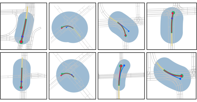
Figure 3: Qualitative results of R-Pred on Argoverse validation set. Yellow, green, blue, and red lines represent the history, ground truth, the initial trajectory proposal with the highest score, and the final (refined) trajectory, respectively. The sky blue region denotes tubular regions used for TQSA. These figures present different vehicle motion scenarios such as continuing straight ahead, turning left, slowing down, changing lanes, etc.

5 Experiments

In this section, we describe the experimental setup used to evaluate the performance of the proposed R-Pred, and present both quantitative and qualitative analyses of the behavior of the model.

Datasets. Both Argoverse [5] and nuScenes [3] datasets provide dynamic agent trajectories and HD-map in real-world driving scenarios. The Argoverse dataset was collected from two US cities, including Miami and Pittsburgh. Each sample contains $5$ seconds trajectories of tracked vehicles sampled at $10$ Hz. Argoverse dataset provides HD-map with detailed lane information. The prediction task is to predict future trajectories for $3$ seconds given past trajectories of $2$ seconds. The dataset contains $205,942$ training, $39,272$ validation, and $78,143$ test samples.

The nuScenes dataset was collected in Boston and Singapore. The collected trajectories are $6$ seconds long and are sampled at $2$Hz. The prediction task is defined as that of predicting future trajectories for $6$ seconds given past trajectories of $2$ seconds. HD-map is also provided along with the trajectory data. The dataset is split into $32,186$ training, $8,560$ validation, and $9,041$ test samples.

Metrics. For the performance evaluation, we adopt widely used performance metrics including average displacement error ($ADE$), final displacement error ($FDE$), and miss rate ($MR$). $ADE$ refers to the mean square error compared to the ground truth over the entire time steps, and $FDE$ is defined as the average displacement error at the endpoint. We evaluate the prediction accuracy with $M>1$ trajectory predictions using $minADE_{M}$ and $minFDE_{M}$, which are the minimum $ADE$ and $FDE$ over $M$ predicted trajectories, respectively. $MR_{M}$ measures the ratio within 2 meters of the endpoint of the best-predicted trajectory and ground truth. We also use brier minimum FDE ($brierFDE_{M}$), which measures the value of $minFDE_{M}+(1-p)^{2}$, where $p$ is corresponding trajectory probability. This imposes a penalty when the probability of the best trajectory is low.

Implementation Details. We set the threshold $\mathcal{D}$ and $\mathcal{T}$ of PIA to 0.1 and $10$ meters and $\tau$ of TQSA to $20$ meters. The embedding size of all features is set to 128 for comparative performance analysis. We used existing prediction architectures for the ITPNet. We chose the structure of [55] on Argoverse and that of [10] on nuScenes. These models achieved excellent performance on both benchmarks. They are considered ITPNet baselines and are used to measure the performance gain achieved by our refinement network. We trained the proposed model on TiTAN RTX GPU for 64 epochs with 32 batch sizes. The data are batched randomly. For all experiments, we trained the model using AdamW optimizer with an initial learning rate of 5e-4. We used cosine annealing to decay the learning rate and applied dropout with a 0.1 ratio. Data augmentation was not used.

ITPNet	PIA	TQSA	$\textit{minADE}_{6}$	$\textit{minFDE}_{6}$	$\textit{MR}_{6}$%
✓			0.694	1.057	10.63
✓	✓		0.677	0.992	9.64
✓	✓	✓	0.657	0.945	8.69

Table 3: Ablation study. Contributions of the main components evaluated on the Argoverse validation set.

5.1 Quantitative Results

Table 1 presents the performance of R-Pred evaluated on Argoverse test set. We compare the performance of R-Pred with that of several top ranked models [51, 53, 41, 29, 14, 30, 19, 16, 34, 45, 15, 49, 43, 33, 55]. R-Pred achieves the best prediction accuracy in terms of the $minADE_{1}$, $minFDE_{1}$, $minADE_{6}$ and $minFDE_{6}$ metrics and competitive performance in terms of $brierFDE_{6}$ and $MR_{6}$. R-Pred sets a new state-of-the-art performance surpassing the current best methods, Wayformer [33] and MultiPath++ [43]. Compared to the ITPNet baseline, the proposed method offers performance improvements of 3.80% and 7.43% in terms of $minADE_{6}$, and $minFDE_{6}$, respectively. This indicates that our trajectory refinement strategy can effectively improve the reliability and robustness of the initial prediction using ITPNet.

Table 2 presents the performance of several motion prediction methods on nuScenes validation set. We compare R-Pred with the top ranked methods [37, 40, 32, 4, 31, 26, 9, 16, 10] on the nuScenes leaderboard. R-Pred achieves significant performance gains compared with other prediction methods. R-Pred exhibits the performance gain of 7.75% and 11.62% in $minADE_{5}$ and $minFDE_{5}$ compared to the ITPNet baseline. These results demonstrate that the proposed two refinement modules have high-quality learning capabilities.

$\tau$	$\textit{minADE}_{6}$	$\textit{minFDE}_{6}$	$\textit{MR}_{6}$%
5	0.659	0.957	8.927
10	0.658	0.952	8.840
20	0.657	0.945	8.698
30	0.657	0.946	8.714
50	0.659	0.954	8.878

Table 4: Ablation study. Performance versus $\tau$ parameter of TQSA evaluated on the Argoverse validation set.

$\mathcal{D}$	$\textit{minADE}_{6}$	$\textit{minFDE}_{6}$	$\textit{MR}_{6}$%
10	0.657	0.945	8.698
20	0.658	0.947	8.730
30	0.659	0.949	8.811
40	0.659	0.950	8.821

Table 5: Ablation study. Performance versus $\mathcal{D}$ parameter of PIA evaluated on the Argoverse validation set.

5.2 Ablation Study

We conducted several ablation studies on the Argoverse validation set. We reduced the training time required to conduct the ablation study by decreasing the feature size from 128 to 64 and increasing the batch size from 32 to 64. The trained model was evaluated on the entire validation set.

Contribution of Each Module. Table 3 shows the contributions of each module to overall performance achieved by R-Pred. We evaluated performance as we added each component one by one. We consider the following three modules of R-Pred: 1) ITPNet baseline, 2) PIA, and 3) TQSA. When the PIA is added to ITPNet baseline, the $minFDE_{6}$ improves by 6.15% and $MR_{6}$ improves by 9.31%. This indicates the effectiveness of inter-agent interaction modeling by PIA. When TQSA is added, it achieves the performance gains of 4.74% and 9.85% in $minFDE_{6}$ and $MR_{6}$. We observe that proposal refinement using local scene context improves the performance significantly. Finally, the combination of PIA and TQSA has improved the performance of ITPNet baseline by 10.6% and 18.25%, in $minFDE_{6}$ and $MR_{6}$, respectively.

Performance Versus $\tau$ and $\mathcal{D}$. We investigated the impact of the parameters $\tau$ and $\mathcal{D}$ on the performance. Recall that $\tau$ and $\mathcal{D}$ are the distance thresholds used in TQSA and PIA, respectively. Table 4 presents the performance of R-Pred evaluated for several values of $\tau=\{5,10,20,30,50\}$. R-Pred performs best at $\tau=20,30$, and degrades as $\tau$ becomes larger or smaller than these values. This is likely due to the fact that when the threshold gets too large, a lot of irrelevant scene context can be used for cross-attribution. Table 5 presents the performance of R-Pred for several values of $\mathcal{D}=\{10,20,30,40\}$. R-Pred achieves the best performance with $\mathcal{D}=10$. Note that increasing the threshold $\mathcal{D}$ above 10 does not improve performance.
Effect of Per-proposal Scene Context Strategy. One of our key innovations is to use the tube-query for pooling the customized scene context for each proposal. We investigated the benefit of our per-proposal feature pooling method. We compare R-Pred with the baseline that shares the global scene context features for all proposals in the refinement step. Table 6 shows that our strategy offers 1.76% and 3.24% performance gains in $minFDE_{6}$ and $MR_{6}$ over the baseline, which confirms the advantage of the proposed per-proposal feature pooling method.

Per-proposal	Shared	$\textit{minADE}_{6}$	$\textit{minFDE}_{6}$	$\textit{MR}_{6}\textit{\%}$
scene context	scene context
	✓	0.662	0.962	8.981
✓		0.657	0.945	8.69

Table 6: Ablation study. Comparison of per-proposal scene context versus shared scene context evaluated on the Argoverse validation set.

5.3 Qualitative Results

Fig. 3 shows a visualization of the actual predicted trajectory samples generated by R-Pred using Argoverse validation set. We visualize the final trajectory with the best score produced by R-Pred (red line) and the corresponding trajectory proposal from ITPNet (blue line). We also include the ground truth trajectory (green line). We added the tubular area used for TQSA to the figure (sky blue region). We observe that our refinement network reduced the prediction error in the trajectories generated by ITPNet. Note that in the third column, our refinement stage modifies the initial trajectory proposal off-road to the trajectory within the road. More qualitative results are provided in Supplementary Material.

6 Conclusions

In this paper, we have proposed a two-stage trajectory prediction method, referred to as R-Pred. We have introduced a novel per proposal trajectory refinement strategy in which each trajectory proposal generated in the first-stage network is refined using contextual information tailored to the proposal. TRNet utilized the local scene context captured by pooling scene component features in a tubular region around the trajectory proposal. TRNet also uses the inter-agent interaction context inferred from a group of influential trajectory proposals of neighboring agents. The results of an experimental evaluation conducted on Argoverse and nuScenes benchmark datasets confirmed that R-Pred significantly outperforms existing methods and achieves state-of-the-art performance in terms of some evaluation metrics.

Supplementary Material

A The Detailed Network Architecture

Fig. 4 presents the detailed network architecture of our R-Pred. The entire network structure consists of ITPNet, TQSA module, PIA module and prediction head. TQSA and PIA take the output of ITPNet as an input and perform scene encoding and interaction encoding for trajectory refinement.

B Additional Ablation Study

Input Formats of TRNet. TRNet is applied to the proposal features for refinement. The trajectory proposals are used only to extract the local scene features and conduct the distance-wise proposal grouping. To verify the advantage of our strategy, we compare our method with the baseline that re-encodes the trajectory proposals through MLP and applies the TRNet to the resulting features. Table 7 shows that by using the proposal features for refinement, our strategy outperforms the baseline by 1.87% and 4.4% in $minFDE_{6}$ and $MR_{6}$. This confirms the benefit of using the proposal features for the refinement network.

Proposal	Trajectory	$\textit{minADE}_{6}$	$\textit{minFDE}_{6}$	$\textit{MR}_{6}\textit{\%}$
feature	re-encoding
	✓	0.666	0.963	9.09
✓		0.657	0.945	8.69

Table 7: Ablation study. Comparison between our strategy and the baseline evaluated on the Argoverse validation set.

C Additional Qualitative Examples

We visualize additional qualitative examples obtained in diverse interaction scenes. The examples were selected from Argoverse validation set. We compare the trajectory samples produced by ITPNet and TRNet to demonstrate the effectiveness of our refinement framework. We present the figures in two columns, where the left figures provide initial trajectory proposals, shown in blue, and the right figures provide the corresponding refined trajectories from TRNet, shown in red. The ground truth is shown as a green line and the trajectories of other agents are shown as black.

Speed Control Scenarios. In Fig. 5, we consider the scenarios where the target agents slow down or accelerate while interacting with other neighboring agent. In these examples, TRNet produces improved predictions by maintaining an appropriate distance from other agents.

Overtaking Scenarios. Fig. 6 shows three cases in which the target agents change lanes to overtake another agents. In all cases, TRNet produces trajectory predictions that are closer to the ground truth than ITPNet.

Intersection Scenarios. Fig. 7 shows the scenarios where the target agents interact with the nearby agents at intersections. Even if the initial trajectory proposals for two neighboring agents conflict, the trajectories in TRNet will not conflict after refinement.

Multi-modal Trajectory Behavior. Fig. 8 shows the multi-modal trajectory samples generated by ITPNet and TRNet. Some of ITPNet’s trajectories do not seem plausible because they fall outside of road boundaries. In contrast, TRNet predicts the trajectories that better fit the scene structures and do not compromise the diversity of trajectory modes.

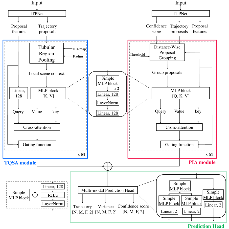
Figure 4: Detailed architecture of R-Pred model.

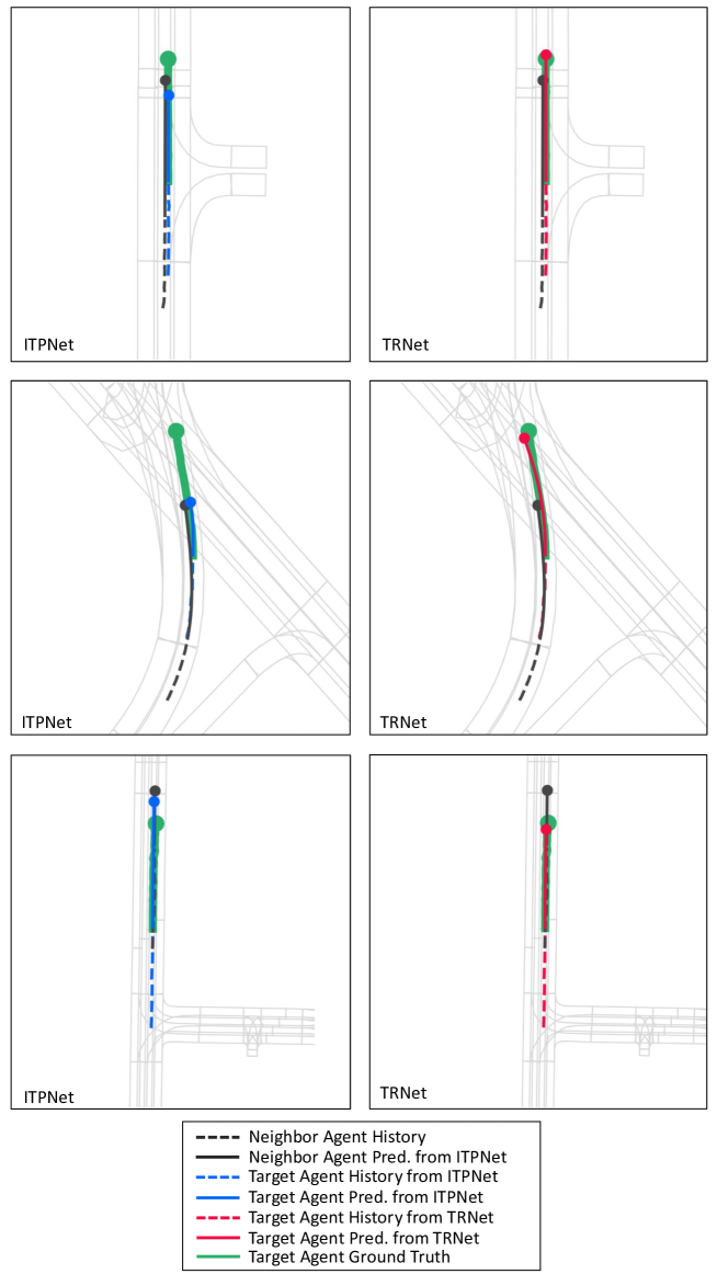
Figure 5: Visualization of trajectories for several speed control scenarios. In these scenarios, the target agents slow down or accelerate while interacting with other agents. The proposed refinement framework generates the predictions improved over the initial proposals from ITPNet.

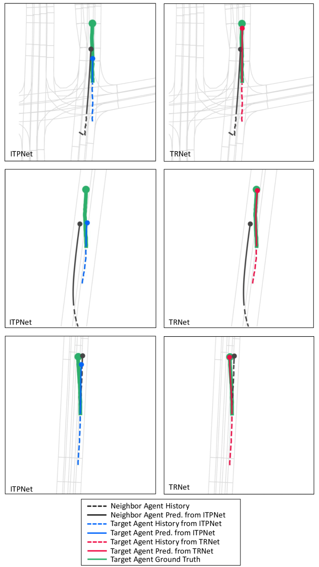
Figure 6: Visualization of trajectories for several overtaking scenarios. In these scenarios, the target agents change lanes to overtake other agents. Considering proposal-level interactions between the agents, TRNet produces trajectory predictions that are closer to the ground truth than ITPNet. Note that conflicts between the initial proposals from two neighboring agents are resolved by the proposed refinement framework.

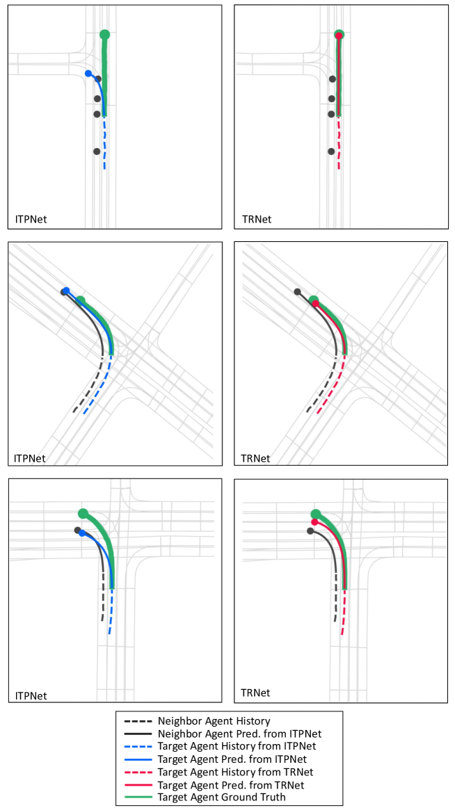
Figure 7: Visualization of trajectories for several intersection scenarios. The target agents interact with the other agents at interactions. For all cases considered, TRNet produces trajectories that do not collide with other trajectories.

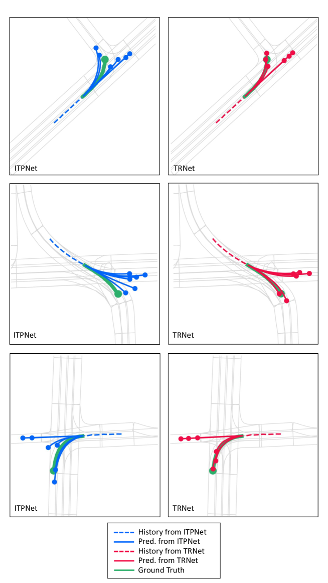
Figure 8: Visualization of multi-modal trajectories obtained by ITPNet and TRNet. The multi-modal trajectories predicted by TRNet mostly conform to the scene structures, whereas some trajectories generated by ITPNet are not physically plausible.

References

- [1] Alexandre Alahi, Kratarth Goel, Vignesh Ramanathan, Alexandre Robicquet, Li Fei-Fei, and Silvio Savarese. Social lstm: Human trajectory prediction in crowded spaces. In In Proceedings of the IEEE conference on computer vision and pattern recognition (CVPR), pages 961–971, 2016.
- [2] Jimmy Lei Ba, Jamie Ryan Kiros, and Geoffrey E Hinton. Layer normalization. arXiv preprint arXiv:1607.06450, 2016.
- [3] Holger Caesar, Varun Bankiti, Alex H Lang, Sourabh Vora, Venice Erin Liong, Qiang Xu, Anush Krishnan, Yu Pan, Giancarlo Baldan, and Oscar Beijbom. nuscenes: A multimodal dataset for autonomous driving. In In Proceedings of the IEEE/CVF conference on computer vision and pattern recognition (CVPR), pages 11621–11631, 2020.
- [4] Yuning Chai, Benjamin Sapp, Mayank Bansal, and Dragomir Anguelov. Multipath: Multiple probabilistic anchor trajectory hypotheses for behavior prediction. In In Conference on Robot Learning (CoRL), pages 86–99, 2020.
- [5] Ming-Fang Chang, John Lambert, Patsorn Sangkloy, Jagjeet Singh, Slawomir Bak, Andrew Hartnett, De Wang, Peter Carr, Simon Lucey, Deva Ramanan, et al. Argoverse: 3d tracking and forecasting with rich maps. In In Proceedings of the IEEE/CVF Conference on Computer Vision and Pattern Recognition (CVPR), pages 8748–8757, 2019.
- [6] Junyoung Chung, Caglar Gulcehre, KyungHyun Cho, and Yoshua Bengio. Empirical evaluation of gated recurrent neural networks on sequence modeling. arXiv preprint arXiv:1412.3555, 2014.
- [7] Henggang Cui, Vladan Radosavljevic, Fang-Chieh Chou, Tsung-Han Lin, Thi Nguyen, Tzu-Kuo Huang, Jeff Schneider, and Nemanja Djuric. Multimodal trajectory predictions for autonomous driving using deep convolutional networks. In In 2019 International Conference on Robotics and Automation (ICRA), pages 2090–2096, 2019.
- [8] Nachiket Deo and Mohan M Trivedi. Convolutional social pooling for vehicle trajectory prediction. In In Proceedings of the IEEE Conference on Computer Vision and Pattern Recognition Workshops (CVPRW), pages 1468–1476, 2018.
- [9] Nachiket Deo and Mohan M Trivedi. Trajectory forecasts in unknown environments conditioned on grid-based plans. arXiv preprint arXiv:2001.00735, 2020.
- [10] Nachiket Deo, Eric Wolff, and Oscar Beijbom. Multimodal trajectory prediction conditioned on lane-graph traversals. In In Conference on Robot Learning (CoRL), pages 203–212, 2022.
- [11] Nemanja Djuric, Vladan Radosavljevic, Henggang Cui, Thi Nguyen, Fang-Chieh Chou, Tsung-Han Lin, Nitin Singh, and Jeff Schneider. Uncertainty-aware short-term motion prediction of traffic actors for autonomous driving. In In Proceedings of the IEEE/CVF Winter Conference on Applications of Computer Vision (WACV), pages 2095–2104, 2020.
- [12] Tharindu Fernando, Simon Denman, Sridha Sridharan, and Clinton Fookes. Soft+ hardwired attention: An lstm framework for human trajectory prediction and abnormal event detection. Neural networks, 108:466–478, 2018.
- [13] Jiyang Gao, Chen Sun, Hang Zhao, Yi Shen, Dragomir Anguelov, Congcong Li, and Cordelia Schmid. Vectornet: Encoding hd maps and agent dynamics from vectorized representation. In In Proceedings of the IEEE/CVF Conference on Computer Vision and Pattern Recognition (CVPR), pages 11525–11533, 2020.
- [14] Thomas Gilles, Stefano Sabatini, Dzmitry Tsishkou, Bogdan Stanciulescu, and Fabien Moutarde. Home: Heatmap output for future motion estimation. In In 2021 IEEE International Intelligent Transportation Systems Conference (ITSC), pages 500–507, 2021.
- [15] Thomas Gilles, Stefano Sabatini, Dzmitry Tsishkou, Bogdan Stanciulescu, and Fabien Moutarde. Gohome: Graph-oriented heatmap output for future motion estimation. In In 2022 International Conference on Robotics and Automation (ICRA), pages 9107–9114, 2022.
- [16] Thomas Gilles, Stefano Sabatini, Dzmitry Tsishkou, Bogdan Stanciulescu, and Fabien Moutarde. Thomas: Trajectory heatmap output with learned multi-agent sampling. In International Conference on Learning Representations (ICLR), 2022.
- [17] Roger Girgis, Florian Golemo, Felipe Codevilla, Martin Weiss, Jim Aldon D’Souza, Samira Ebrahimi Kahou, Felix Heide, and Christopher Pal. Latent variable sequential set transformers for joint multi-agent motion prediction. In In International Conference on Learning Representations (ICLR), 2021.
- [18] Ross Girshick. Fast r-cnn. In In Proceedings of the IEEE/CVF International Conference on Computer Vision (ICCV), pages 1440–1448, 2015.
- [19] Junru Gu, Chen Sun, and Hang Zhao. Densetnt: End-to-end trajectory prediction from dense goal sets. In In Proceedings of the IEEE/CVF International Conference on Computer Vision (ICCV), pages 15303–15312, 2021.
- [20] Agrim Gupta, Justin Johnson, Li Fei-Fei, Silvio Savarese, and Alexandre Alahi. Social gan: Socially acceptable trajectories with generative adversarial networks. In In Proceedings of the IEEE conference on computer vision and pattern recognition (CVPR), pages 2255–2264, 2018.
- [21] Kaiming He, Georgia Gkioxari, Piotr Dollár, and Ross Girshick. Mask r-cnn. In In Proceedings of the IEEE/CVF International Conference on Computer Vision (ICCV), pages 2961–2969, 2017.
- [22] Kaiming He, Xiangyu Zhang, Shaoqing Ren, and Jian Sun. Deep residual learning for image recognition. In In Proceedings of the IEEE conference on computer vision and pattern recognition (CVPR), pages 770–778, 2016.
- [23] Sepp Hochreiter and Jürgen Schmidhuber. Long short-term memory. Neural computation, 9(8):1735–1780, 1997.
- [24] Boris Ivanovic and Marco Pavone. The trajectron: Probabilistic multi-agent trajectory modeling with dynamic spatiotemporal graphs. In In Proceedings of the IEEE/CVF International Conference on Computer Vision (ICCV), pages 2375–2384, 2019.
- [25] ByeoungDo Kim, Chang Mook Kang, Jaekyum Kim, Seung Hi Lee, Chung Choo Chung, and Jun Won Choi. Probabilistic vehicle trajectory prediction over occupancy grid map via recurrent neural network. In 2017 IEEE 20th International Conference on Intelligent Transportation Systems (ITSC), pages 399–404, 2017.
- [26] ByeoungDo Kim, Seong Hyeon Park, Seokhwan Lee, Elbek Khoshimjonov, Dongsuk Kum, Junsoo Kim, Jeong Soo Kim, and Jun Won Choi. Lapred: Lane-aware prediction of multi-modal future trajectories of dynamic agents. In In Proceedings of the IEEE/CVF Conference on Computer Vision and Pattern Recognition (CVPR), pages 14636–14645, 2021.
- [27] Sumit Kumar, Yiming Gu, Jerrick Hoang, Galen Clark Haynes, and Micol Marchetti-Bowick. Interaction-based trajectory prediction over a hybrid traffic graph. In In 2021 IEEE/RSJ International Conference on Intelligent Robots and Systems (IROS), pages 5530–5535, 2021.
- [28] Namhoon Lee, Wongun Choi, Paul Vernaza, Christopher B Choy, Philip HS Torr, and Manmohan Chandraker. Desire: Distant future prediction in dynamic scenes with interacting agents. In In Proceedings of the IEEE conference on computer vision and pattern recognition (CVPR), pages 336–345, 2017.
- [29] Ming Liang, Bin Yang, Rui Hu, Yun Chen, Renjie Liao, Song Feng, and Raquel Urtasun. Learning lane graph representations for motion forecasting. In In European Conference on Computer Vision (ECCV), pages 541–556, 2020.
- [30] Yicheng Liu, Jinghuai Zhang, Liangji Fang, Qinhong Jiang, and Bolei Zhou. Multimodal motion prediction with stacked transformers. In In Proceedings of the IEEE/CVF Conference on Computer Vision and Pattern Recognition (CVPR), pages 7577–7586, 2021.
- [31] Chenxu Luo, Lin Sun, Dariush Dabiri, and Alan Yuille. Probabilistic multi-modal trajectory prediction with lane attention for autonomous vehicles. In In 2020 IEEE/RSJ International Conference on Intelligent Robots and Systems (IROS), pages 2370–2376, 2020.
- [32] Kaouther Messaoud, Nachiket Deo, Mohan M Trivedi, and Fawzi Nashashibi. Trajectory prediction for autonomous driving based on multi-head attention with joint agent-map representation. In In 2021 IEEE Intelligent Vehicles Symposium (IV), pages 165–170, 2021.
- [33] Nigamaa Nayakanti, Rami Al-Rfou, Aurick Zhou, Kratarth Goel, Khaled S Refaat, and Benjamin Sapp. Wayformer: Motion forecasting via simple & efficient attention networks. arXiv preprint arXiv:2207.05844, 2022.
- [34] Jiquan Ngiam, Vijay Vasudevan, Benjamin Caine, Zhengdong Zhang, Hao-Tien Lewis Chiang, Jeffrey Ling, Rebecca Roelofs, Alex Bewley, Chenxi Liu, Ashish Venugopal, et al. Scene transformer: A unified architecture for predicting future trajectories of multiple agents. In In International Conference on Learning Representations (ICLR), 2022.
- [35] Seong Hyeon Park, ByeongDo Kim, Chang Mook Kang, Chung Choo Chung, and Jun Won Choi. Sequence-to-sequence prediction of vehicle trajectory via lstm encoder-decoder architecture. In 2018 IEEE Intelligent Vehicles Symposium (IV), pages 1672–1678, 2018.
- [36] Seong Hyeon Park, Gyubok Lee, Jimin Seo, Manoj Bhat, Minseok Kang, Jonathan Francis, Ashwin Jadhav, Paul Pu Liang, and Louis-Philippe Morency. Diverse and admissible trajectory forecasting through multimodal context understanding. In In European Conference on Computer Vision (ECCV), pages 282–298, 2020.
- [37] Tung Phan-Minh, Elena Corina Grigore, Freddy A Boulton, Oscar Beijbom, and Eric M Wolff. Covernet: Multimodal behavior prediction using trajectory sets. In In Proceedings of the IEEE/CVF Conference on Computer Vision and Pattern Recognition (CVPR), pages 14074–14083, 2020.
- [38] Shaoqing Ren, Kaiming He, Ross Girshick, and Jian Sun. Faster r-cnn: Towards real-time object detection with region proposal networks. Advances in neural information processing systems, 28, 2015.
- [39] Amir Sadeghian, Vineet Kosaraju, Ali Sadeghian, Noriaki Hirose, Hamid Rezatofighi, and Silvio Savarese. Sophie: An attentive gan for predicting paths compliant to social and physical constraints. In In Proceedings of the IEEE/CVF conference on computer vision and pattern recognition (CVPR), pages 1349–1358, 2019.
- [40] Tim Salzmann, Boris Ivanovic, Punarjay Chakravarty, and Marco Pavone. Trajectron++: Dynamically-feasible trajectory forecasting with heterogeneous data. In In European Conference on Computer Vision (ECCV), pages 683–700, 2020.
- [41] Haoran Song, Di Luan, Wenchao Ding, Michael Y Wang, and Qifeng Chen. Learning to predict vehicle trajectories with model-based planning. In Conference on Robot Learning, pages 1035–1045, 2022.
- [42] Nitish Srivastava, Geoffrey Hinton, Alex Krizhevsky, Ilya Sutskever, and Ruslan Salakhutdinov. Dropout: a simple way to prevent neural networks from overfitting. The journal of machine learning research, 15(1):1929–1958, 2014.
- [43] Balakrishnan Varadarajan, Ahmed Hefny, Avikalp Srivastava, Khaled S Refaat, Nigamaa Nayakanti, Andre Cornman, Kan Chen, Bertrand Douillard, Chi Pang Lam, Dragomir Anguelov, et al. Multipath++: Efficient information fusion and trajectory aggregation for behavior prediction. In In 2022 International Conference on Robotics and Automation (ICRA), pages 7814–7821, 2022.
- [44] Ashish Vaswani, Noam Shazeer, Niki Parmar, Jakob Uszkoreit, Llion Jones, Aidan N Gomez, Łukasz Kaiser, and Illia Polosukhin. Attention is all you need. Advances in neural information processing systems, 30, 2017.
- [45] Jingke Wang, Tengju Ye, Ziqing Gu, and Junbo Chen. Ltp: Lane-based trajectory prediction for autonomous driving. In In Proceedings of the IEEE/CVF Conference on Computer Vision and Pattern Recognition (CVPR), pages 17134–17142, 2022.
- [46] David Wu and Yunnan Wu. for interaction prediction. arXiv preprint arXiv:2111.08184, 2021.
- [47] Chenxin Xu, Maosen Li, Zhenyang Ni, Ya Zhang, and Siheng Chen. Groupnet: Multiscale hypergraph neural networks for trajectory prediction with relational reasoning. In In Proceedings of the IEEE/CVF Conference on Computer Vision and Pattern Recognition (CVPR), pages 6498–6507, 2022.
- [48] Yi Xu, Lichen Wang, Yizhou Wang, and Yun Fu. Adaptive trajectory prediction via transferable gnn. In In Proceedings of the IEEE/CVF Conference on Computer Vision and Pattern Recognition (CVPR), pages 6520–6531, 2022.
- [49] Maosheng Ye, Tongyi Cao, and Qifeng Chen. Tpcn: Temporal point cloud networks for motion forecasting. In Proceedings of the IEEE/CVF Conference on Computer Vision and Pattern Recognition, pages 11318–11327, 2021.
- [50] Ye Yuan, Xinshuo Weng, Yanglan Ou, and Kris M Kitani. Agentformer: Agent-aware transformers for socio-temporal multi-agent forecasting. In In Proceedings of the IEEE/CVF International Conference on Computer Vision (ICCV), pages 9813–9823, 2021.
- [51] Wenyuan Zeng, Ming Liang, Renjie Liao, and Raquel Urtasun. Lanercnn: Distributed representations for graph-centric motion forecasting. In 2021 IEEE/RSJ International Conference on Intelligent Robots and Systems (IROS), pages 532–539, 2021.
- [52] Lingyao Zhang, Po-Hsun Su, Jerrick Hoang, Galen Clark Haynes, and Micol Marchetti-Bowick. Map-adaptive goal-based trajectory prediction. In In Conference on Robot Learning (CoRL), pages 1371–1383, 2021.
- [53] Hang Zhao, Jiyang Gao, Tian Lan, Chen Sun, Ben Sapp, Balakrishnan Varadarajan, Yue Shen, Yi Shen, Yuning Chai, Cordelia Schmid, et al. Tnt: Target-driven trajectory prediction. In In Conference on Robot Learning (CoRL), pages 895–904, 2021.
- [54] Tianyang Zhao, Yifei Xu, Mathew Monfort, Wongun Choi, Chris Baker, Yibiao Zhao, Yizhou Wang, and Ying Nian Wu. Multi-agent tensor fusion for contextual trajectory prediction. In In Proceedings of the IEEE/CVF Conference on Computer Vision and Pattern Recognition (CVPR), pages 12126–12134, 2019.
- [55] Zikang Zhou, Luyao Ye, Jianping Wang, Kui Wu, and Kejie Lu. Hivt: Hierarchical vector transformer for multi-agent motion prediction. In In Proceedings of the IEEE/CVF Conference on Computer Vision and Pattern Recognition (CVPR), pages 8823–8833, 2022.