A Dichotomy Theorem for Linear Time Homomorphism Orbit Counting in Bounded Degeneracy Graphs

Abstract

Counting the number of homomorphisms of a pattern graph $H$ in a large input graph $G$ is a fundamental problem in computer science. There are myriad applications of this problem in databases, graph algorithms, and network science. Often, we need more than just the total count. Especially in large network analysis, we wish to compute, for each vertex $v$ of $G$, the number of $H$-homomorphisms that $v$ participates in. This problem is referred to as homomorphism orbit counting, as it relates to the orbits of vertices of $H$ under its automorphisms.

Given the need for fast algorithms for this problem, we study when near-linear time algorithms are possible. A natural restriction is to assume that the input graph $G$ has bounded degeneracy, a commonly observed property in modern massive networks. Can we characterize the patterns $H$ for which homomorphism orbit counting can be done in linear time?

We discover a dichotomy theorem that resolves this problem. For pattern $H$, let $\ell$ be the length of the longest induced path between any two vertices of the same orbit (under the automorphisms of $H$). If $\ell\leq 5$, then $H$-homomorphism orbit counting can be done in linear time for bounded degeneracy graphs. If $\ell>5$, then (assuming fine-grained complexity conjectures) there is no near-linear time algorithm for this problem. We build on existing work on dichotomy theorems for counting the total $H$-homomorphism count. Somewhat surprisingly, there exist (and we characterize) patterns $H$ for which the total homomorphism count can be computed in linear time, but the corresponding orbit counting problem cannot be done in near-linear time.

1 Introduction

The problem of analyzing the occurrences of a small pattern graph $H$ in a large input graph $G$ is a central problem in computer science. The theoretical study has led a rich and immensely deep theory [37, 18, 28, 22, 38, 2, 21, 43, 49]. The applications of graph pattern counts occur across numerous scientific area, including logic, biology, statistical physics, database theory, social sciences, machine learning, and network science [32, 17, 20, 16, 25, 13, 27, 40, 57, 43, 23, 42]. (Refer to the tutorial [51] for more details on applications.)

A common formalism used for graph pattern counting is homomorphism counting. The pattern simple graph is denoted $H=(V(H),E(H))$, and is thought of constant-sized. The input simple graph is denoted $G=(V(G),E(G))$. An $H$-homomorphism is a map $f:V(H)\to V(G)$ that preserves edges. Formally, $\forall(u,v)\in E(H)$, $(f(u),f(v))\in E(G)$. Let $\mathrm{Hom}_{H}(G)$ denote the number of distinct $H$-homomorphisms in $G$.

Given the importance of graph homomorphism counts, the study of efficient algorithms for this problem is almost a subfield in of itself [33, 3, 16, 25, 24, 22, 13, 21, 14, 49]. The simplest version of this problem is when $H$ is a triangle, itself a problem that attracts much attention. Let $n=|V(G)|$ and $k=|V(H)|$. Computing $\mathrm{Hom}_{H}(G)$ is $\#W[1]$-hard when parameterized by $k$ (even when $H$ is a $k$-clique), so we do not expect $n^{o(k)}$ algorithms for general $H$ [22]. Much of algorithmic study of homomorphism counting is in understanding conditions on $H$ and $G$ when the trivial $n^{k}$ running time bound can be beaten.

Our work is inspired by the challenges of modern applications of homomorphism counting, especially in network science. Typically, $n$ is extremely large, and only near linear algorithms are feasible. So our first motivation is to understand natural conditions under which homomorphism counting can be done in near linear time. Inspired by a long history and recent theory on this topic, we focus on bounded degeneracy input graphs. Many practical algorithms for large-scale graph pattern counting use algorithms for bounded degeneracy graphs [2, 36, 43, 41, 35, 42]. Real-world graphs typically have a small degeneracy, comparable to their average degree ([30, 35, 53, 5, 9], also Table 2 in [5]).

Secondly, many modern applications for homomorphism counting require more finer grained statistics that just the global count $\mathrm{Hom}_{H}(G)$. The aim is to find, for every vertex $v$ of $G$, the number of homomorphisms that $v$ participates in. Seminal work in network analysis for bioinformatics plots the distributions of these per-vertex counts to compare graphs [34, 44]. Orbit counts can be used to generate features for vertices, sometimes called the graphlet kernel [52]. In the past few years, there have been many applications of these per-vertex counts [10, 57, 50, 55, 4, 56, 48, 58, 59].

Algorithms for this problem require considering the "roles" that $v$ could play in a homomorphism. For example, in a path of length $6$, there are $4$ different roles: a vertex $v$ could be in the middle, could be at the end, or two other positions. These roles are colored in Fig. 1. A formalism for this problem requires looking at the automorphisms of $H$; we give the mathematical definitions in the next subsection. The roles are called orbits, and the problem of $H$-homomorphism orbit counting is as follows: for every orbit $\psi$ in $H$ and every vertex $v$ in $G$, output the number of homomorphisms of $H$ where $v$ participates in the orbit $\psi$. This is the main question addressed by our work:

What are the pattern graphs $H$ for which the $H$-homomorphism orbit counting problem is computable in near-linear time (when $G$ has bounded degeneracy)?

Recent work of Bressan followed by Bera-Pashanasangi-Seshadhri introduced the question of homomorphism counting for bounded degeneracy graphs, from a fine-grained complexity perspective [14, 8]. A dichotomy theorem for linear time counting of $\mathrm{Hom}_{H}(G)$ was provided in subsequent work [6]. Assuming fine-grained complexity conjectures, $\mathrm{Hom}_{H}(G)$ can be computed in near-linear time iff the longest induced cycle of $H$ has length at most $5$. It is natural to ask whether these results extend to orbit counting.

1.1 Main Result

We begin with some preliminaries. The input graph $G=(V,E)$ has $n$ vertices and $m$ edges. A graph $G$ is $\kappa$-degenerate if the minimum degree in every subgraph of $G$ is at most $\kappa$; the degeneracy of $G$ is the minimum value of $\kappa$ such that $G$ is $\kappa$-degenerate. A family of graphs has bounded degeneracy if the degeneracy is constant with respect to graph size. Bounded degeneracy graph classes are extremely rich. For example, all minor-closed families have bounded degeneracy; preferential attachment graphs also have bounded degeneracy; real-world graphs have a small value of degeneracy (often in the 10s) with respect to their size (often in the hundreds of millions) [5].

In our results, we consider the pattern graph $H$ to have constant size. Consider the group of automorphisms of $H$. The vertices of $H$ can be partitioned into orbits, which consist of vertices that be mapped to each other by some automorphism. For example, in Fig. 1, the $7$-path has four different orbits, where each orbit has the same color. The $7$-path with a hanging triangle (in Fig. 1) has many more orbits, since the opposite “ends” of the $7$-path cannot be mapped by a non-trivial automorphism.

The set of orbits of pattern $H$ is denoted $\Psi(H)$. Let $\Phi(H,G)$ be the set of homomorphisms of $H$ in $G$. We now define our main problem.

Definition 1.1.

Orbit Homomorphism Counts: For each orbit $\psi\in\Psi(H)$ and vertex $v\in V$, define $OrbitHom_{H,\psi}(v)$ to be the number of $H$-homomorphisms mapping a vertex of $\psi$ to $v$. Formally, $OrbitHom_{H,\psi}(v)=|\{\phi\in\Phi(G,H)\ |\exists u\in\psi,\ \ \phi(u)=v\}|$.

The problem of $H$-homomorphism orbit counting is to output the values $OrbitHom_{H,\psi}(v)$ for all $v\in V,\psi\in\Psi(H)$. (Abusing notation, ${OrbitHom}_{{H}}({G})$ refers to the set of all of these values.)

Note that for a given $H$, the size of the output is $n|\Psi(H)|$. For example, when $H$ is the $7$-path, we will get $4n$ counts, for each vertex and each of the four orbits.

Our main result is a dichotomy theorem that precisely characterizes patterns $H$ for which $OrbitHom_{H}(G)$ can be computed in near-linear time. We introduce a key definition.

Definition 1.2.

For a pattern $H$, the Longest Induced Path Connecting Orbits of $H$, denoted $LIPCO(H)$ is defined as follows. It is the length of the longest induced simple path, measured in edges, between any two vertices $h,h^{\prime}$ in $H$ (where $h$ may be equal to $h^{\prime}$) in the same orbit.

Again refer to Fig. 1. The $7$-path has a LIPCO of six, since the ends are in the same orbit. On the other hand, the pattern to the right ($7$-path with a triangle) has a LIPCO of one, from the path/edge between the ends of the triangle.

Our main theorem proves that the LIPCO determines the dichotomy.

Theorem 1.3.

Let $G$ be a graph with $n$ vertices, $m$ edges, and degeneracy $\kappa$. Let $f:\mathbb{N}\rightarrow\mathbb{N}$ denote some explicit function. Let $\gamma>0$ denote the constant from the Triangle Detection Conjecture (Conjecture 1.4).

• If $LIPCO(H)\leq 5$: there exists a deterministic algorithm that computes $OrbitHom_{H}(G)$ in time $f(\kappa)O(m\log n)$

• If $LIPCO(H)>5$: assume the Triangle Detection Conjecture. For any function $g:\mathbb{N}\rightarrow\mathbb{N}$, there is no algorithm with (expected) running time $g(\kappa)O(m^{1+\gamma})$ that computes $OrbitHom_{H}(G)$.

The Triangle Detection Conjecture was introduced by Abboud and Williams on the complexity of determining whether a graph has a triangle [1]. It is believed that this problem cannot be solved in near-linear, and indeed, may even require $\Omega(m^{4/3})$ time.

Conjecture 1.4 (Triangle Detection Conjecture [1]).

There exists a constant $\gamma>0$ such that in the word RAM model of $O(\log n)$ bits, any algorithm to detect whether an input graph on $m$ edges has a triangle requires $\Omega(m^{1+\gamma})$ time in expectation.

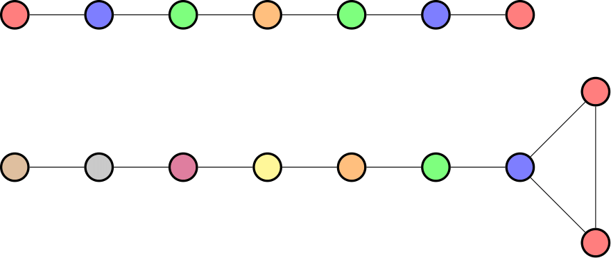
Figure 1: Examples of Orbits and LIPCO values. Vertices in the same orbit have the same color. The top graph is the $7$-path, so the edge length is $6$. There is an induced path of length $6$ between the red vertices, hence the LIPCO of this graph is $6$. Theorem 1.3 implies that we can not compute $OrbitHom$ in near-linear time.
The bottom graph adds a triangle at the end, and the only vertices in the same orbit in that graph are the blue ones. The LIPCO is now less than 6 in this graph so we can compute $OrbitHom$ in near-linear time.

1.1.1 Orbit Counting vs Total Homomorphism Counting

In the following discussion, we use "linear" to really mean near-linear, we assume that the Triangle Detection Conjecture is true, and we assume that $G$ has bounded degeneracy.

One of the most intriguing aspects of the dichotomy of Theorem 1.3 is that it differs significantly from the condition for getting the total homomorphism count. As mentioned earlier, the inspiration for Theorem 1.3 is the analogous result for determining $\mathrm{Hom}_{H}(G)$. There is a near-linear time algorithm iff the length of the longest induced cycle (LICL) of $H$ is at most five. Since the definition of LIPCO considers induced cycles (induced path between a vertex to itself), if $LIPCO(H)\leq 5$, then $LICL(H)\leq 5$. This implies, not surprisingly, that the total homomorphism counting problem is easier than the orbit counting problem.

But there exist patterns $H$ for which the orbit counting problem is provably harder than total homomorphism counting. And a simple example is the $7$-path (path with $7$ vertices). There is a simple linear time dynamic program for counting the homomorphism of paths. But the endpoints are in same orbit, so the LIPCO is six, and Theorem 1.3 proves the non-existence of linear time algorithms for orbit counting. On the other hand, the LIPCO of the $6$-path is five, so orbit counting can be done in linear time.

Consider the pattern in the bottom of Fig. 1. The LICL is three, so the total homomorphism count can be determined in linear time. Because the ends of the underlying $7$-path lie in different orbits, the LIPCO is also three (by the triangle). Theorem 1.3 provides a linear time algorithm for orbit counting.

We hope that this discussion highlights the potential for rich mathematics (and the surprises) in the study of homomorphism counting on bounded degeneracy graphs.

1.2 Main Ideas

The starting point for homomorphism counting on bounded degeneracy graphs is the seminal work of Chiba-Nishizeki on using acyclic graph orientations [18]. It is known that, in linear time, the edges of a bounded degeneracy graph can be acyclically oriented while keeping the outdegree bounded [39]. For clique counting, we can now use a brute force algorithm in all out neighborhoods, and get a linear time algorithm. Over the past decade, various researchers observed that this technique can generalize to certain other pattern graphs [19, 43, 41, 42]. Given a pattern $H$, one can add the homomorphism counts of all acyclic orientations of $H$ in the oriented $G$. In certain circumstances, each acyclic orientation can be efficiently counted by a carefully tailored dynamic program that breaks the oriented $H$ into subgraphs spanned by rooted, directed trees.

Bressan gave a unified treatment of this approach through the notion of DAG tree decompositions. These decompositions give a systematic way of breaking up an oriented pattern $H$ into smaller pieces, such that homomorphism counts can be constructed by a dynamic program. Bera et al. showed that if the LICL of $H$ is at most $5$, then the DAG treewidth of $H$ is at most one [8, 6]. This immediately implies Bressan’s algorithm runs in linear time.

Our result on orbit counting digs deeper into ithe mechanics of Bressan’s algorithm. Firstly, note that Bressan’s algorithm must necessarily compute "compressed" data structures that store information about homomorphism counts. For example, the DAG tree based algorithm can count $4$-cycles in linear time for bounded degeneracy graphs (this was known from Chiba-Nishizeki as well [18]). But there could exist quadratically many $4$-cycles in such a graph. Consider two vertices connected by $\Theta(n)$ disjoint paths of length $2$; each pair of paths yields a distinct $4$-cycle. Any linear time algorithm for $4$-cycle counting has to carefully index directed paths and combine these counts, without actually touching every $4$-cycle.

By carefully looking at Bressan’s algorithm, we discover that "local" per-vertex information about $H$-homomorphisms can be read out. Using the DAG tree decomposition, one can combine these counts into a quantity that looks like orbit counts. Unfortunately, we cannot get exact orbit counts, but rather a kind of weighted version. For any orbit $\psi$ and vertex $v$ in $G$, we get a weighted sum over homomorphisms mapping $\psi$ to $v$, where the weight of an $H$-homomorphism is proportional to the number of vertices of $H$ that are mapped to $v$.

To extract exact orbit counts, we design an inclusion-exclusion formula that essentially "inverts" the weight sum (or linear combination) into the desired count. This formula requires orbits counts for other patterns $H^{\prime}$, which can be constructed by merging vertices in the same orbit of $H$.

Based on previous results, we can prove that if the LICL of all these $H^{\prime}$ patterns is at most $5$, then $OrbitHom_{H}(G)$ can be computed in (near)linear time. This LICL condition over all $H^{\prime}$ is equivalent to the LIPCO of $H$ being at most $5$. We achieve the upper bound of Theorem 1.3.

What is remarkable is that the above seemingly ad hoc algorithm optimally characterizes when orbit counting is linear time computable. To prove the matching lower bound, we use tools from the breakthrough work of Curticapean-Dell-Marx [21]. They prove that the complexity of counting linear combinations of homomorphism counts is determined by the hardest individual count (up to polynomial factors). Gishboliner-Levanzov-Shapira give a version of this tool for proving linear time hardness [29]. Consider a pattern $H$ with LIPCO at least six. We can construct a pattern $H^{\prime}$ with LICL at least six by merging vertices of an orbit in $H$. We use the tools above to construct a constant number of linear sized graphs $G_{1},G_{2},\ldots,G_{k}$ such that a linear combination of $H$-orbit counts on these graphs yields the total $H^{\prime}$-homomorphism count on $G$. The latter problem is hard by existing bounds, and hence the hardness bounds translate to $OrbitHom_{H}(G)$.

2 Related Work

Homomorphism and subgraph counting on graphs is an immense topic with an extensive literature in theory and practice. For a detailed discussion of practical applications, we refer the reader to a tutorial [51].

Homomorphism counting is intimately connected with the treewidth of the pattern $H$. The notion of tree decomposition and treewidth were introduced in a seminal work by Robertson and Seymour [45, 46, 47]; although it has been discovered before under different names [11, 31]. A classic result of Dalmau and Jonsson [22] proved that $\mathrm{Hom}_{H}(G)$ is polynomial time solvable if and only if $H$ has bounded treewidth, otherwise it is $\#W[1]$-complete. Díaz et al [24] gave an algorithm for homomorphism counting with runtime $O(2^{k}n^{t(H)+1})$ where $t(H)$ is the treewidth of the target graph $H$.

To improve on these bounds, recent work has focused on restrictions on the input $G$ [49]. A natural restriction is bounded degeneracy, which is a nuanced measure of sparsity introduced by early work of Szekeres-Wilf [54]. Many algorithmic results exploit low degeneracy for faster subgraph counting problems [18, 26, 2, 36, 43, 41, 35, 42].

Pioneering work of Bressan introduced the concept of DAG treewidth for faster algorithms for homomorphism counting in bounded degeneracy graphs [14]. Bressan gave an algorithm for counting $\mathrm{Hom}_{H}(G)$ running in time essentially $m^{\tau(H)}$, where $\tau$ denotes the DAG treewidth. The result also proves that (assuming ETH) there is no algorithm running in time $m^{o(\tau(H)/\log\tau(H))}$.

Bera-Pashanasangi-Seshadhri build on Bressan’s methods to discover a dichotomy theorem for linear time homomorphism counting in bounded degeneracy graphs [7, 8]. Gishboliner, Levanzov, and Shapira independently proved the same characterization using slightly different methods [29, 6].

We give a short discussion of the Triangle Detection Conjecture. Itai and Rodeh [33] gave the first non-trivial algorithm for the triangle detection and finding problem with $O(m^{3/2})$ runtime. The current best known algorithm runs in time $O(\min\{n^{\omega},m^{{2\omega}/{(\omega+1)}}\})$ [3], where $\omega$ is the matrix multiplication exponent. Even for $\omega=2$, the bound is $m^{4/3}$ and widely believed to be a lower bound. Many classic graph problems have fine-grained complexity hardness based on Triangle Detection Conjecture [1].

Homomorphism or subgraph orbit counts have found significant use in network analysis and machine learning. Przulj introduced the use of graphlet (or orbit count) degree distributions in bioinformatics [44]. The graphlet kernel of Shervashidze-Vishwanathan-Petri-Mehlhorn-Borgwardt uses vertex orbits counts to get embeddings of vertices in a network [52]. Four vertex subgraph and large cycle and clique orbit counts have been used for discovering special kinds of vertices and edges [57, 48, 58, 59]. Orbits counts have been used to design faster algorithms for finding dense subgraphs in practice [10, 50, 55, 4, 56].

3 Preliminaries

We use $G$ to denote the input graph and $H$ to denote the pattern graph, both $G=(V,E)$ and $H=(V_{H},E_{H})$ are simple, undirected and connected graph. We denote $|V|$ and $|E|$ by $n$ and $m$ respectively and $|V_{H}|$ by $k$.

A pattern graph $H$ is divided into orbits, we use the definition from Bondy and Murty (Chapter $1$, Section $2$ [12]):

Definition 3.1.

Fix labeled graph $H=(V(H),E(H))$. An automorphism is a bijection $\sigma:V(H)\to V(H)$ such that $(u,v)\in E(H)$ iff $(\sigma(u),\sigma(v))\in E(H)$.

Define an equivalence relation among $V(H)$ as follows. We say that $u\sim v\ (u,v\in V(H))$ iff there exists an automorphism that maps $u$ to $v$. The equivalence classes of the relation are called orbits.

We refer with $\Psi(H)$ (or $\Psi$ if $H$ is clear in the context) to the set of orbits in $H$, we refer to individual orbits in $H$ with $\psi$. Note that every vertex $u\in H$ belongs to exactly one orbit. In Fig. 2 we can see examples of different graphs with their separate orbits.

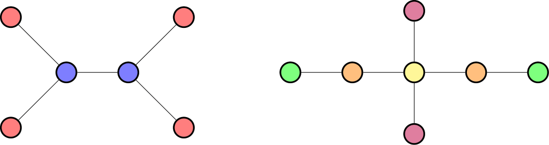
Figure 2: An example of two graphs where the orbits are represented using different colors.

A Homomorphism from $H$ to $G$ is defined as a mapping $\pi:V(H)\to V(G)$ such that for all $(u,v)\in E(H)$ we have that $(\pi(u),\pi(v))\in E(G)$. We refer with $\Phi(H,G)$ to the set of homomorphisms of $H$ in $G$.

We use $Hom_{H}$ for the problem of counting homomorphism of $H$. We refer with $Hom_{H}(G)$ for the same problem with the input graph $G$.

We use $OrbitHom_{H}$ for the problem of obtaining Orbit Homormorphism Counts of a pattern $H$. We refer with $OrbitHom_{H}(G)$ for the same problem with the input graph $G$. When we want to refer to the orbit counts for a specific orbit $\psi$ in $H$ we use $OrbitHom_{H,\psi}$ and $OrbitHom_{H,\psi}(G)$, when we want the counts in relation to a specific vertex $v$ in $G$ we will use $OrbitHom_{H}(v)$ or $OrbitHom_{H,\psi}(v)$.

We say that a graph $G$ is $k$-degenerate if each non-empty subgraph of $G$ has minimum vertex degree of at most $k$. The degeneracy of $G$, denoted by $\kappa(G)$ or $\kappa$ is the smallest integer $k$ for which $G$ is $k$-degenerate.

Acyclic orientations:

We will use acyclic orientations in order to obtain the vertex homomorphism counts. Given a vertex ordering $\prec$ of a graph $G$, we can obtain a DAG $G^{\to}_{\prec}$ by orienting each edge $\{u,v\}\in E$ from $u$ to $v$ if $u\prec v$.

The degeneracy ordering of a graph is an ordering $\prec$ obtained by repeatedly removing the minimum degree vertex from a graph. This ordering has the property that every vertex in $G^{\to}_{\prec}$ will have an out degree of at most $\kappa$. We will refer to the this degeneracy oriented graph $G$ as simply $G^{\to}$.

We will also orient acyclically $H$, we will refer with $P$ to the dag orientations of $H$ and $\Sigma(H)$ to the set of all dag orientation of $H$.

Dag tree decomposition:

Bressan [14] introduced the concept of dag tree decomposition in order to decompose the pattern graph and compute the homomorphisms. Let $D$ be a DAG and $S\subseteq V$ be the set of source vertices in $D.$ For a source vertex $s\in S$, let $\text{reachable}_{D}(s)$ denote the set of vertices in $D$ that are reachable from $s$. For a subset of the sources $B\subseteq S$, let $\text{reachable}_{D}(B)=\bigcup_{s\in B}\text{reachable}_{D}(s)$.

Definition 3.2.

(DAG tree decomposition [14]). Let $D$ be a DAG with source vertices $S$. A DAG tree decomposition of D is a tree $T=(\mathcal{B},\mathcal{E})$ with the following three properties:

1. Each node $B\in\mathcal{B}$ (referred to as a “bag” of sources) is a subset of the source vertices $S$: $B\subseteq S$.

2. The union of the nodes in $T$ is the entire set $S$: $\bigcup_{B\in\mathcal{B}}B=S$.

3. For all $B,B_{1},B_{2}\in\mathcal{B}$, if $B$ lies on the unique path between the nodes $B_{1}$ and $B_{2}$ in $T$, then $\text{reachable}(B_{1})\cap\text{reachable}(B_{2})\subseteq\text{reachable}(B)$.

Bressan [14] also introduces the concept of dag-treewidth $\tau$, where $\tau(T)=\max_{B\in\mathcal{B}}|B|$, and for a dag $D$ we have that $\tau(D)$ is the minimum $tau(T)$ for all valid DAG tree decompositions $T$ of $D$.

Bressan’s algorithm for computing homomorphism counts:

Bressan introduced an algorithm that allows to compute the homomorphisms counts taking advantage of the the DAG tree decomposition [15]. The algorithm is recursive as it runs in one of the nodes of the DAG decomposition and calls its children. We will refer at this algorithm as "Bressan’s algorithm" or $HomCount(P,T,B)$. Let $P$ be a DAG, $T=(\mathcal{B},\mathcal{E})$ a DAG Tree Decomposition for $P$ and $B$ any vertex in $\mathcal{B}$, We will refer with $P(B)$ to the graph induced in $P$ by $\text{reachable}(B)$. Let $\Gamma(B)$ be the down-closure of $B$ in $T$, we will refer with $P(\Gamma(B))$ to the graph induced in $P$ by $\text{reachable}(\Gamma(B))$, note that if $B$ is the root of $T$, then $P(\Gamma(B))=P$.

Bressan [15] proved the following Lemma regarding $HomCount(P,T,B)$:

Lemma 3.3.

Lemma 5 in [15]: Let $P$ be any dag, $T=(\mathcal{B},\mathcal{E})$ any d.t.d. for $P$, and $B$ any element of $\mathcal{B}$. $HomCount(P,T,B)$ in time $O(|\mathcal{B}|poly(k)d^{k-\tau(T)}n^{\tau(T)}\log n)$ returns a dictionary $C_{B}$ that for all $\phi_{B}:P(B)\to G$ satisfies $C_{B}(\phi_{B})=hom(P(\Gamma[B]),G,\phi_{B})$.

Where $hom(P(\Gamma[B]),G,\phi_{B})$ it is the number of homomorphisms of $P(\Gamma[B])$ in $G$ restricted to $\phi_{B}$. Formally this means that:

$$C_{B}(\phi_{B})=|\phi\in\Phi(P(\Gamma(B)),G^{\to}):\ \forall\ u\in P(B)\ \phi(u)=\phi_{B}(u)|\ \ \forall\phi_{B}\in\Phi(P(B),G)$$ (1)

In the case that $B$ is the root of $T$ this is equivalent to:

$$C_{B}(\phi_{B})=|\phi\in\Phi(P,G^{\to}):\ \forall\ u\in P(B)\ \phi(u)=\phi_{B}(u)|\ \ \forall\ \phi_{B}\in\Phi(P(B),G)$$ (2)

We will make use of this, running the algorithm multiple times to obtain the Vertex Homomorphism Counts.

Largest Induced Cycle Length and dag-treewidth:

Bera-Pashanasangi-Seshadhri (Theorem 4.1 in [8]) showed that there is a clear direction between the Largest Induced Cycle Length in a graph and its dag-treewidth. In fact $\tau(H)=1$ only if $LICL(H))\leq 5$.

4 Obtaining Vertex Homomorphism Counts

We first define a "simpler" version of orbits counts, where we simply ignore orbits. For any vertex $h\in H$ and vertex $v\in V$, we count the number of homomorphisms that map $h$ to $v$.

Definition 4.1.

Vertex Homomorphism Counts: For each vertex $h\in V_{H}$ and vertex $v\in V$, it is the count of homomorphisms $\phi$ of $H$ in $G$ such that $\phi$ maps $h$ to $v$. we will call $\textbf{VertexHom}_{\textbf{H}}(\textbf{G})$ to the problem of finding those counts, formally, $\forall\ h\in V_{H},v\in V\text{ we have }VertexHom_{H,h}(v)=|\phi\in\Phi(G,H):\phi(h)=v|$.

The main theorems of this section follows.

Theorem 4.2.

Given a graph $G$ and a pattern $H$ we can compute $VertexHom_{H}(G)$ in time $f(k)\cdot O(\kappa^{k-\tau}n^{\tau}\log{n})$, where $\tau$ is the dag-treewidth of $H$.

Theorem 4.3.

Given a bounded degeneracy graph $G$ and a pattern $H$ with Largest Induced Cycle Length(LICL) $\leq 5$ we can compute $VertexHom_{H}(G)$ in time $f(k)\cdot O(n\log{n})$.

The proof for Theorem 4.3 comes directly from Theorem 4.2, as from Bera et al.[8] showed that if a graph has a $LICL\leq 5$ then its dag-treewidth $\tau$ is 1. So it suffices to prove Theorem 4.2.

To compute $VHC_{H,G}$ we will orient $G$ acyclically using the degeneracy, let $G^{\to}$ be the result of orienting $G$ using the degeneracy orientation. Let $\Sigma(H)$ be the set of the possible dag orientations of $H$. We have the following lemma:

Lemma 4.4.

$VertexHom_{H}(G)=\sum_{P\in\Sigma(H)}VertexHom_{P}(G^{\to})$

Proof 4.5.

When orienting $G$ each homomorphism of $H$ in $G$ must be now a homomorphism of one and only one of the orientations $P\in\Sigma(H)$. Hence we can obtain the vertex counts for each of the dag orientations and then aggregate the entire counts.

Hence the problem is reduced to counting $VertexHom_{P}(G^{\to})$ for all orientations $P\in\Sigma(H)$. To achieve it we need to use the dag tree decomposition showed in [14]. This will allow us to divide the dag $P$ into smaller paths, then we can use Bressan’s algorithm [15] to obtain the counts efficiently using Dynamic Programming. In Equation 2 we saw that the output of Bressan’s algorithm is a dictionary $C_{B}$ containing the number of homomorphism of $P$ in $G^{\to}$ that match any of the homomorphism of $P(B)$ in $G^{\to}$.

If we aggregate the counts in $C_{B}$ for each vertex $u\in P(B)$ we will actually be obtaining the counts of the number of homomorphism of $H$ in $G$ where $u$ is mapped to each vertex in $G$.

Because we can arbitrarily set the root of the DAG tree decomposition of $P$, we could run Bressan’s algorithm for each the possible roots of the DAG tree decomposition. If for each dictionary we aggregate the counts for each of the nodes in $P(B)$ we will end up with a dictionary that for each vertex $u\in H$ and vertex $v\in G$ contains the number of homomorphisms of $H$ in $G$ such that $u$ is mapped to $v$.

We will formalize this approach in Algorithm 1 that gives us the following lemma:

Algorithm 1 $VertexHom_{P}(G^{\to})$

1:Let $Counts$ be an empty dictionary

2:Compute a minimum dag-treewidth dag tree decomposition $T=(\mathcal{B},\mathcal{E})$ for $P$

3:for $B\in\mathcal{B}$ do

4:     Let $T^{\prime}$ be a rearrangement of $T$ with $B$ as root.

5:     Use Bressan’s algorithm to compute $C_{B}$=HomCount($P,T^{\prime},B$)

6:     for vertex $u\in V_{P}(B)$ do

7:         if $u$ not in $Counts$ then

8:              Let $AGG_{u}$ be an empty dictionary with default 0

9:              for every key $\phi$ in $C_{B}$ do

10:                  Let $v$ be $\phi(u)$

11:                  $AGG_{u}(v)+=C_{B}(\phi)$

12:              end for

13:              Let $Counts(u)=AGG_{u}$

14:         end if

15:     end for

16:end for

17:Return $Counts$

Lemma 4.6.

Algorithm 1 runs in time $O(poly(k)\kappa^{k-\tau(P)}n^{\tau(P)}\log{n})$ and returns a dictionary $Counts$, such that $Counts(u)=VertexHom_{P,u}(G^{\to})$ for each vertex $u\in P$ .

Proof 4.7.

First, we prove the time complexity of the algorithm. Let $T=(\mathcal{B},\mathcal{E})$ be the minimum dag-treewidth dag tree composition for $P$. We will have $|\mathcal{B}|=O(k)$ iterations of the main loop. In each iteration we are running Bressan’s Algorithm, from Lemma 3.3 this will take $O(|\mathcal{B}|poly(k)\kappa^{k-\tau(T)}n^{\tau(T)}\log{n})$, because we are using a DAG tree composition with minimum dag-treewidth we have that $\tau(T)=\tau(P)$ and also $|\mathcal{B}|=O(k)$, hence each loop will take $O(poly(k)\kappa^{k-\tau(P)}n^{\tau(P)}\log{n})$.

Finally, we need to consider the time to aggregate the counts in each iteration of the loop, this will take time $O(poly(k)|C_{B}|\log{n})$, as we are iterating over each key in $C_{B}$ and each vertex in $P(B)$, with $\log{n}$ being the cost of accessing the dictionary. Lemma $4$ of [15] shows that $|C_{B}|=O(d^{k-|B|}n^{|B|})$, and we have $|B|=O(\tau(T))$. Hence the total complexity of the algorithm will be $O(poly(k)\kappa^{k-\tau(P)}n^{\tau(P)}\log{n})$.

Now we prove the correctness of the algorithm. First we show that the algorithm will update the value of $Counts$ for each vertex $u\in P$. In each iteration of the for loop we will update the vertices in $V_{P}(B)$, we are doing this for all the bags $B\in\mathcal{B}$, hence we will update all the vertices in $\bigcup_{B\in\mathcal{B}}V_{P}{B}$, from the Definition 3.2 we have that $\bigcup_{B\in\mathcal{B}}B=S_{P}$, for any dag $P=P(S_{P})$, hence we will be iterating over all vertices in $P$.

Lastly, we need to show that $Counts(u)=VertexHom_{P,u}(G^{\to})$. From Lemma 3.3 and Equation 2 we have that $C_{B}(\Phi)$ contains the number of homomorphisms of $P$ in $G$ restricted to $\phi$. If we only consider one of the vertices $u$ in $V_{P}(B)$ and aggregate the counts of $C_{B}$ we will obtain the number of homomorphisms of $P$ in $G$ restricted to $u$, which exactly corresponds to $VertexHom_{P,u}(G^{\to})$.

We can finally proceed to prove the upper bound for Vertex Homomorphism Counts:

Proof 4.8 (Proof of Theorem 4.2).

In Lemma 4.6 show that we can compute $VertexHom_{P}(G^{\to})$ using Algorithm 1 in $O(poly(k)\kappa^{k-\tau(P)}n^{\tau(P)}\log{n})$ time.

We can repeat this process for every acyclic orientation of $H$, and combine the counts as in Lemma 4.4 to obtain the total counts of $VertexHom_{H}(G)$. Because the number of acyclic orientations of $H$, $|\Sigma(H)|$ is bounded by $2^{O(k\log{k})}$, we can obtain the counts in time $f(k)O(\kappa^{k-\tau(P)}n^{\tau(P)}\log{n})$.

5 Obtaining Orbit Homomorphism Counts

Our focus moves now to computing Orbit Homomorphism Counts. If we just add the counts of $VertexHom_{H,u}(G)$ for the vertices $u\in\psi$, we could count the same homomorphism multiple times. This happens if there are two or more vertices in $\psi$ that are mapped to the same vertex in $V$.

A way of dealing with this situation is to compute vertex counts for patterns where we combine different vertices in the same orbit $\psi$ of $H$. Let $S\subseteq\psi$ be a subset of vertices of the same orbit, we will call $H/S$ to the graph resulting of combining the vertices in $S$ into a single vertex, removing any double edge. We can calculate $VertexHom_{H/S,S}(v)$, that is, the number of homomorphisms of $H/S$ in $G$ that map the new vertex $S$ to $v$. We can show this counts is equivalent to the number of homomoprhisms of $H$ in $G$ that map all the vertices in $S$ to $v$, if $S$ is an independent set:

Lemma 5.1.

If $S$ is an independent set and not empty:

$$VertexHom_{H/S,S}(v)=|\phi\in\Phi(H,G):\ \forall\ u\in S\ \phi(u)=v|$$

Proof 5.2.

We can show that there is a 1 to 1 mapping of homomorphisms $\phi$ of $H$ to $G$ that map all vertices in $S$ to $v$ to homomorphisms $\phi^{\prime}$ of $H/S$ to $G$ that map $S$ to $v$. When $S$ is an independent set.

First, giving $\phi$ we can obtain $\phi^{\prime}$ by setting $\phi^{\prime}(u)=\phi(u)$ for all vertices $u\in H\setminus S$, and $\phi(S)=v$. We can show that this is a homomorphism of $H/S$, let $u,w$ be an edge in $H/S$, if $(u,w)\in H\setminus S$ then $(\phi^{\prime}(u),\phi^{\prime}(w))=(\phi(u),\phi(w))\in E$, otherwise one of the vertices has to be $S$, without loss of generality we say $w=S$, hence $(\phi^{\prime}(u),\phi^{\prime}(w))=(\phi(u),v)\in E$, as there has to be an edge connecting $\phi(u)$ to $v$ or $\phi$ would not be an homomorphism of $H$ in $G$.

Now we prove the opposite operation, given $\phi^{\prime}$ we can obtain $\phi$ by setting $\phi(u)=\phi^{\prime}(u)$ for all vertices $u\in H\setminus S$, and $\phi(u)=v$ for all vertices $u\in S$. We prove $\phi$ is a homomorphism of $H$, for every edge $(u,w)$ in $H$, if $u,w\notin S$, then $(\phi(u),\phi(w))=(\phi^{\prime}(u),\phi^{\prime}(w))\in E$, otherwise without loss of generality $w\in S$, thus $(\phi(u),\phi(w))=(\phi^{\prime}(u),\phi^{\prime}(S))\in E$.

Given an orbit $\psi$, let $\mathcal{S}(\psi)$ be the set of all non empty sets of sets $S\subseteq\psi$ such that $S$ is an independent set. We can combine these counts as in the following lemma:

Lemma 5.3.

$$OrbitHom_{H,\psi}(v)=\sum_{S\in\mathcal{S}(\psi)}(-1)^{|S|+1}VertexHom_{H/S,S}(v)$$

Proof 5.4.

Using Lemma 5.1 we have that:

$$\sum_{S\in\mathcal{S}(\psi)}(-1)^{|S|+1}VertexHom_{H/S,S}(v)=\sum_{S\in\mathcal{S}(\psi)}(-1)^{|S|+1}|\phi\in\Phi(H,G):\ \forall\ u\in S\ \phi(u)=v|$$

Hence, the sum will only be affected by the different homomorphism $\phi$ of $H$ in $G$. Suffices to prove that any homomorphism will contribute to the total sum with $1$ if maps an vertex in $\psi$ to $v$, and with $0$ otherwise.

Let $\phi$ be a homomorphism of $H$ in $G$, let $S$ be the set of vertices in $u\in\psi$ that are mapped to $v$, note that $S$ must be an independent set, as adjacent vertices can not be mapped to the same vertex in $G$. Clearly if $S=\emptyset$ then it will not affect the sum and hence any homomorphism that doesn’t map a vertex $u\in\psi$ to $v$ will contribute with $0$ to the total sum.

If $S$ is non empty, it will increase the count in all the terms for any non empty subset $S^{\prime}\subseteq S$, we can show that the total contribution of $\phi$ will be:

$$\begin{split}\text{Contribution}(\phi)=\sum_{S^{\prime}\subseteq S:S^{\prime}\neq\emptyset}(-1)^{|S^{\prime}|+1}=\sum_{i=1}^{|S|}(-1)^{i+1}\binom{|S|}{i}\\ =\sum_{i=1}^{|S|}(-1)^{i+1}\left(\binom{|S|-1}{i-1}+\binom{|S|-1}{i}\right)=\binom{|S|-1}{0}+(-1)^{|S|+1}\binom{|S|-1}{|S|}=1\end{split}$$

Thus, we finally have:

$$\begin{split}\sum_{S\in\mathcal{S}(\psi)}(-1)^{|S|+1}|\phi\in\Phi(H,G):\ \forall\ u\in S\ \phi(u)=v|\\ =|\phi\in\Phi(G,H):\exists u\in\psi\ \ \phi(u)=v|=OrbitHom_{H,\psi}(v)\end{split}$$

Hence, we can calculate the vertex counts for all the graphs $H/S$ and combine them to obtain $OrbitHom_{H}(G)$. To analyze the time complexity necessary to compute all the counts we will introduce the following definition:

Definition 5.5.

Max Orbit Dag-treewidth ($\tau_{\Psi}(H)$): It is the maximum Dag-treewidth between all the possible $S\subseteq\psi$ for all $\psi\in H$ such that $S$ is a non-empty independent set.

$$\tau_{\Psi}(H)=\max_{\psi\in H}\max_{S\in\mathcal{S}(\psi)}\tau(H/S)$$

Theorem 5.6.

Given a graph $G$ and a pattern $H$ we can compute $OrbitHom_{H}(G)$ in time $f(k)\cdot O(\kappa^{k-\tau_{\psi}}n^{\tau_{\psi}}\log{n})$, where $\tau_{\psi}$ is the Max Orbit Dag-Treewidth of $H$.

Proof 5.7.

Using Lemma 5.3 we can compute $OrbitHom_{H}(G)$ from the individual counts of $VertexHom_{H/S}(G)$. We can compute all the vertex counts as we will have at most $2^{k}$ sets $S$. The time complexity will be dominated by the instance of $VertexHom_{H/S}(G)$ for which $\tau(H/S)$ is the largest, which is exactly $\tau_{\psi}(H)$.

However the conditions under $\tau_{\psi}$ is $1$ are not the same than $\tau$, it is easy to come with an example of a graph with $LICL\leq 5$ for which $\tau_{\psi}>1$. For example, in the 7-path graph (Fig. 1), combining the vertices in the exterior orbit gives a 6-cycle graph, which clearly has a LICL of $6$. For this purpose we introduced the concept of Longest Induced Path Connecting Orbits (LIPCO) in Definition 1.2. We can prove the following:

Lemma 5.8.

A graph $H$ will have $\tau_{\psi}(H)=1$ if and only if $LIPCO(H)\leq 5$.

Proof 5.9.

First, if $LIPCO(H)>6$ then we can show that $\tau_{\psi}(H)>1$. Let $u,w\in\psi$ be the two ends of the longest induced path, we have two cases. If $u=w$ then we clearly have an induced cycle of length $6$ or more in $H$ including the vertex $u$. In that case $tau(H)>1$, and for any $S\subseteq\psi$ with $|S|=1$ we have that $H/S=H$, hence $\tau_{\psi}(H)>1$.

In the other case $u,w$ are distinct vertices, hence we have an induced path of length $6$ or more between them. If $(u,w)\in E_{H}$ then we have that there exists an induced cycle in $H$ of length at least $7$ and $tau(H)>1$. Otherwise, consider the set $S=\{u,w\}$, clearly $S\in\mathcal{S}(\psi)$, consider $H/S$, because we are combining $u,w$ into a single vertex, the induced path that we had will be come an induced cycle, which implies $\tau(H/S)>1$ and $\tau_{\psi}(H)>1$.

Now we need to prove that if $\tau_{\psi}(H)>1$, then $LIPCO(H)>5$. If $\tau_{\psi}(H)>1$ then for some $\psi\in H$ we have a set $S\in\mathcal{S}(\psi)$ such that $\tau(H/S)>1$. If $|S|=1$, then we will have that $H/S=H$ and $\tau(H)>1$ which means that there is a cycle in $H$ of length at least $6$, any vertex in that induced cycle will induced a path of the same length with that vertex in both ends, which implies $LIPCO(H)>5$. If $|S|>1$, if $\tau(H)=1$ then there must be an induced cycle of length at least $6$ in $H/S$ that contains the vertex resultant of merging the vertices of $S$, if we break that vertex back into separate vertices, there will be two vertices $u,w\in S$ that are inducing a path of the same length, and hence, $LIPCO(H)>5$.

Hence, as it happened with $\tau$ we have a threshold on the value of $\tau_{\psi}$ depending on $LIPCO{}$. We can then prove the following theorem:

Theorem 5.10.

Given a bounded degeneracy graph $G$ and a pattern $H$ with Longest Induced Path Connecting Orbits (LIPCO) $\leq 5$ we can compute $OrbitHom_{H}(G)$ in time $f(k)\cdot O(n\log{n})$.

Proof 5.11.

This comes immediately from combining Theorems 5.6 and Lemma 5.8.

This concludes the proof of the upper bound for Theorem 1.3.

6 Lower Bound for computing Orbit Homomorphism Counts

In this section we will prove the lower bound of Theorem 1.3. It will be given by the following theorem:

Theorem 6.1.

Let $H$ be a pattern graph on $k$ vertices with $LIPCO(H)>5$. Assuming the Triangle Detection Conjecture, there exists an absolute constant $\gamma>0$ such that for any function $f:\mathbb{N}\times\mathbb{N}\rightarrow\mathbb{N}$, there is no (expected) $f(\kappa,k)O(m^{1+\gamma})$ algorithm for the $OrbitHom$ problem, where $m$ and $\kappa$ are the number of edges and the degeneracy of the input graph, respectively.

In order to prove this lower bound we will make use of the Lemma $4.2$ from [6]:

Lemma 6.2.

Lemma 4.2 from [6]: Let $H_{1},...,H_{k}$ be pairwise non-isomorphic graphs and let $c_{1},...,c_{k}$ be non-zero constants. For every graph $G$ there are graphs $G_{1},...,G_{K}$, computable in time $O(|V(G)|+|E(G)|)$, such that $|V(Gi)|=O(|V(G)|)$ and $|E(Gi)|=O(|E(G)|)$ for every $i=1,...,k$, and such that knowing $bj:=c_{1}\cdot hom_{H_{1}}(G_{j})+...+c_{k}\cdot hom_{H_{k}}(,G_{j})$ for every $j=1,...,k$ allows one to compute $hom(H_{1},G),...,hom(H_{k},G)$ in time $O(1)$. Furthermore, if $G$ is $O(1)$-degenerate, then so are $G1,...,Gk$.

We will show to express $OrbitHom$ as a linear combination of homomorphism counts, allowing us to apply this lemma in a similar way as the proof of Lemma $4.3$ in [6]. First, we show the following lemma regarding Vertex Homomorphism Counts:

Lemma 6.3.

$$\sum_{v\in V}VertexHom_{H,u}(v)=Hom_{H}(G)\ \ \forall u\in V_{H}$$

Proof 6.4.

$$\begin{split}\sum_{v\in V}VertexHom_{H,u}(v)=\sum_{v\in V}|\phi\in\Phi:\phi(u)=v|=\left|\phi\in\Phi:\phi(u)\in V\right|=\left|\Phi\right|=Hom_{H}(G)\end{split}$$

We will make use of the previous two lemmas to show the following. Let $Agg(H,G,\psi)=\sum_{v\in V}OrbitHom_{H,\psi}(v)$, we will have:

Lemma 6.5.

For every graph $H$ and every orbit $\psi\in H$, there is $k=k(H)$ such that the following holds. For every graph $G$ there are some graphs $G_{1},...,G_{k}$, computable in time $O(|V(G)|+|E(G)|)$, such that $|V(G_{i})|=O(|V|)$ and $|E(G_{i})|=O(|E|)$ for all $i=1,...,k$, and such that knowing $Agg(H,G_{i},\psi),...,Agg(H,G_{k},\psi)$ allows one to compute $Hom_{H/S}(G)$ for all non-empty $S\in\mathcal{S}(\psi)$, in time $O(1)$. Furthermore, if $G$ is $O(1)$-degenerate, then so are $G_{1},...,G_{k}$.

Proof 6.6.

Let $H_{1},...,H_{k}$ be an enumeration of all the graphs $H/S$ for all non-null $S\subseteq\psi$ such that $S$ is not an independent set, up to isomorphism. This means that $H_{i},...,H_{k}$ are pairwise non-isomorphic and $\{H_{1},...,H_{k}\}=\{H/S:S\in\mathcal{S}(\psi)\}$. Let $f(i)$ be equal to the number of $S\in\mathcal{S}(\psi)$ such that $H/S$ is an isomorphism of $H_{i}$ with sign equal to $(-1)^{|S|+1}$, clearly all such $S$ must have the same $|S|$.

Let $G$ be a graph, we can express $Agg(G,H,\psi)$ as follows:

$$\begin{split}Agg(H,G,\psi)=\sum_{v\in V}OrbitHom_{H,\psi}(v)\\ =\sum_{v\in V}\sum_{S\in\mathcal{S}(\psi)}(-1)^{|S|+1}VertexHom_{H/S,S}(v)\\ =\sum_{v\in V}\sum_{i=1}^{k}f(i)VertexHom_{H_{i},S}(v)\\ =\sum_{i=1}^{k}f(i)\sum_{v\in V}VertexHom_{H_{i},S}(v)=\sum_{i=1}^{k}f(i)Hom_{H_{i}}(G)\end{split}$$

Where, the last equality comes from Lemma 6.3.

Hence, we have that $Agg(H,G,\psi)$ is a linear combination of homomorphism counts of $H_{1},...,H_{k}$, we can then use Lemma 6.2 to reach the result of the lemma.

This lemma allows us to finally prove the lower bound for the $OrbitHom$ problem:

Proof 6.7 (Proof of Theorem 6.1).

We prove by contradiction. Given a graph $G$ and a pattern $H$ suppose there exists an algorithm that allows us to compute $OrbitHom_{H}(G)$ in time $f(\kappa,k)O(m)$, then we could use Lemma 6.5 to construct the graphs $G_{1},...,G_{k}$, we can then compute $OrbitHom_{H}(G_{i})$ for all of these graphs in time $f(\kappa,k)O(m)$ and that allows us to trivially obtain $Agg(H,G_{i},\psi)$ for all $G_{i}$ and all $\psi\in H$.

Using the Lemma 6.5 that means that we can compute $Hom_{H/S}(G)$ for all non-empty $S\subseteq\psi$ for all $\psi\in H$ such that $S$ is an independent set. However, if $LIPCO{}>5$ then we will have that $\tau_{\psi}(H)>1$, hence there exists some $S\subseteq\psi$ for some $\psi\in H$ such that $\tau(H/S)>1$, which by Theorem $5.1$ of [6] implies that there will not be an algorithm that computes $Hom_{H/S}(G)$ in time $f(\kappa,k)O(m^{1+\gamma})$ for some $\gamma>0$, which leads to a contradiction.

Combining Theorems 5.10 and 6.1 we finally prove the Main Theorem 1.3, and we have a clear threshold between the instances that we can solve in nearly linear time and the ones that we can not for the Orbit Homomorphism Count problem.

References

- [1] Amir Abboud and Virginia Vassilevska Williams. Popular conjectures imply strong lower bounds for dynamic problems. In Proc. 55th Annual IEEE Symposium on Foundations of Computer Science, 2014.
- [2] Nesreen K. Ahmed, Jennifer Neville, Ryan A. Rossi, and Nick Duffield. Efficient graphlet counting for large networks. In Proceedings of International Conference on Data Mining (ICDM), 2015.
- [3] Noga Alon, Raphael Yuster, and Uri Zwick. Finding and counting given length cycles. Algorithmica, 17(3):209–223, 1997.
- [4] A. Benson, D. F. Gleich, and J. Leskovec. Higher-order organization of complex networks. Science, 353(6295):163–166, 2016.
- [5] Suman K Bera, Amit Chakrabarti, and Prantar Ghosh. Graph coloring via degeneracy in streaming and other space-conscious models. In International Colloquium on Automata, Languages and Programming, 2020.
- [6] Suman K. Bera, Lior Gishboliner, Yevgeny Levanzov, C. Seshadhri, and Asaf Shapira. Counting subgraphs in degenerate graphs. Journal of the ACM, 69(3), 2022.
- [7] Suman K Bera, Noujan Pashanasangi, and C Seshadhri. Linear time subgraph counting, graph degeneracy, and the chasm at size six. In Proc. 11th Conference on Innovations in Theoretical Computer Science. Schloss Dagstuhl-Leibniz-Zentrum für Informatik, 2020.
- [8] Suman K. Bera, Noujan Pashanasangi, and C. Seshadhri. Near-linear time homomorphism counting in bounded degeneracy graphs: The barrier of long induced cycles. 2021.
- [9] Suman K Bera and C Seshadhri. How the degeneracy helps for triangle counting in graph streams. In Principles of Database Systems, pages 457–467, 2020.
- [10] Jonathan W. Berry, Bruce Hendrickson, Randall A. LaViolette, and Cynthia A. Phillips. Tolerating the community detection resolution limit with edge weighting. Phys. Rev. E, 83:056119, May 2011.
- [11] Umberto Bertele and Francesco Brioschi. On non-serial dynamic programming. J. Comb. Theory, Ser. A, 14(2):137–148, 1973.
- [12] JA Bondy and USR Murty. Graph theory (2008). Grad. Texts in Math, 2008.
- [13] Christian Borgs, Jennifer Chayes, László Lovász, Vera T Sós, and Katalin Vesztergombi. Counting graph homomorphisms. In Topics in discrete mathematics, pages 315–371. Springer, 2006.
- [14] Marco Bressan. Faster subgraph counting in sparse graphs. In 14th International Symposium on Parameterized and Exact Computation (IPEC 2019). Schloss Dagstuhl-Leibniz-Zentrum fuer Informatik, 2019.
- [15] Marco Bressan. Faster algorithms for counting subgraphs in sparse graphs. Algorithmica, 83:2578–2605, 2021.
- [16] Graham R Brightwell and Peter Winkler. Graph homomorphisms and phase transitions. Journal of combinatorial theory, series B, 77(2):221–262, 1999.
- [17] Ashok K Chandra and Philip M Merlin. Optimal implementation of conjunctive queries in relational data bases. In Proc. 9th Annual ACM Symposium on the Theory of Computing, pages 77–90, 1977.
- [18] Norishige Chiba and Takao Nishizeki. Arboricity and subgraph listing algorithms. SIAM Journal on Computing, 14:210–223, 1985.
- [19] Jonathan Cohen. Graph twiddling in a mapreduce world. Computing in Science & Engineering, 11(4):29, 2009.
- [20] J. Coleman. Social capital in the creation of human capital. American Journal of Sociology, 94:S95–S120, 1988. URL: http://www.jstor.org/stable/2780243.
- [21] Radu Curticapean, Holger Dell, and Dániel Marx. Homomorphisms are a good basis for counting small subgraphs. In Proceedings of the 49th Annual ACM SIGACT Symposium on Theory of Computing, pages 210–223, 2017.
- [22] Víctor Dalmau and Peter Jonsson. The complexity of counting homomorphisms seen from the other side. Theor. Comput. Sci., 329(1-3):315–323, 2004.
- [23] Holger Dell, Marc Roth, and Philip Wellnitz. Counting answers to existential questions. In Proc. 46th International Colloquium on Automata, Languages and Programming. Schloss Dagstuhl-Leibniz-Zentrum fuer Informatik, 2019.
- [24] Josep Díaz, Maria Serna, and Dimitrios M Thilikos. Counting h-colorings of partial k-trees. Theor. Comput. Sci., 281(1-2):291–309, 2002.
- [25] Martin Dyer and Catherine Greenhill. The complexity of counting graph homomorphisms. Random Structures & Algorithms, 17(3-4):260–289, 2000.
- [26] David Eppstein. Arboricity and bipartite subgraph listing algorithms. Information processing letters, 51(4):207–211, 1994.
- [27] G. Fagiolo. Clustering in complex directed networks. Phys. Rev. E, 76:026107, Aug 2007. URL: http://link.aps.org/doi/10.1103/PhysRevE.76.026107, doi:10.1103/PhysRevE.76.026107.
- [28] Jörg Flum and Martin Grohe. The parameterized complexity of counting problems. SIAM J. Comput., 33(4):892–922, 2004.
- [29] Lior Gishboliner, Yevgeny Levanzov, and Asaf Shapira. Counting subgraphs in degenerate graphs, 2020. arXiv:2010.05998.
- [30] G. Goel and J. Gustedt. Bounded arboricity to determine the local structure of sparse graphs. In International Workshop on Graph-Theoretic Concepts in Computer Science, pages 159–167. Springer, 2006.
- [31] Rudolf Halin. S-functions for graphs. Journal of geometry, 8(1-2):171–186, 1976.
- [32] P. Holland and S. Leinhardt. A method for detecting structure in sociometric data. American Journal of Sociology, 76:492–513, 1970.
- [33] Alon Itai and Michael Rodeh. Finding a minimum circuit in a graph. SIAM Journal on Computing, 7(4):413–423, 1978.
- [34] Shalev Itzkovitz, Reuven Levitt, Nadav Kashtan, Ron Milo, Michael Itzkovitz, and Uri Alon. Coarse-graining and self-dissimilarity of complex networks. 71(016127), January 2005.
- [35] Shweta Jain and C Seshadhri. A fast and provable method for estimating clique counts using turán’s theorem. In Proceedings, International World Wide Web Conference (WWW), pages 441–449, 2017.
- [36] Madhav Jha, C Seshadhri, and Ali Pinar. Path sampling: A fast and provable method for estimating 4-vertex subgraph counts. In Proc. 24th Proceedings, International World Wide Web Conference (WWW), pages 495–505. International World Wide Web Conferences Steering Committee, 2015.
- [37] László Lovász. Operations with structures. Acta Mathematica Academiae Scientiarum Hungarica, 18(3-4):321–328, 1967.
- [38] László Lovász. Large networks and graph limits, volume 60. American Mathematical Soc., 2012.
- [39] David W Matula and Leland L Beck. Smallest-last ordering and clustering and graph coloring algorithms. J. ACM, 30(3):417–427, 1983.
- [40] Derek O’Callaghan, Martin Harrigan, Joe Carthy, and Pádraig Cunningham. Identifying discriminating network motifs in youtube spam. arXiv preprint arXiv:1202.5216, 2012.
- [41] Mark Ortmann and Ulrik Brandes. Efficient orbit-aware triad and quad census in directed and undirected graphs. Applied network science, 2(1):13, 2017.
- [42] Noujan Pashanasangi and C Seshadhri. Efficiently counting vertex orbits of all 5-vertex subgraphs, by evoke. In Proc. 13th International Conference on Web Search and Data Mining (WSDM), pages 447–455, 2020.
- [43] Ali Pinar, C Seshadhri, and Vaidyanathan Vishal. Escape: Efficiently counting all 5-vertex subgraphs. In The Web Conference (WWW), pages 1431–1440. International World Wide Web Conferences Steering Committee, 2017.
- [44] Natasa Przulj. Biological network comparison using graphlet degree distribution. Bioinformatics, 23(2):177–183, 2007.
- [45] Neil Robertson and Paul D Seymour. Graph minors. i. excluding a forest. Journal of Combinatorial Theory, Series B, 35(1):39–61, 1983.
- [46] Neil Robertson and Paul D Seymour. Graph minors. iii. planar tree-width. Journal of Combinatorial Theory, Series B, 36(1):49–64, 1984.
- [47] Neil Robertson and Paul D. Seymour. Graph minors. ii. algorithmic aspects of tree-width. Journal of algorithms, 7(3):309–322, 1986.
- [48] Rahmtin Rotabi, Krishna Kamath, Jon M. Kleinberg, and Aneesh Sharma. Detecting strong ties using network motifs. In The Web Conference (WWW), pages 983–992, 2017. doi:10.1145/3041021.3055139.
- [49] Marc Roth and Philip Wellnitz. Counting and finding homomorphisms is universal for parameterized complexity theory. In Proc. 31st Annual ACM-SIAM Symposium on Discrete Algorithms, pages 2161–2180, 2020.
- [50] Ahmet Erdem Sariyuce, C. Seshadhri, Ali Pinar, and Umit V. Catalyurek. Finding the hierarchy of dense subgraphs using nucleus decompositions. In The Web Conference (WWW), pages 927–937, 2015. URL: http://doi.acm.org/10.1145/2736277.2741640, doi:10.1145/2736277.2741640.
- [51] C. Seshadhri and Srikanta Tirthapura. Scalable subgraph counting: The methods behind the madness: WWW 2019 tutorial. In Proceedings of the Web Conference (WWW), 2019.
- [52] Nino Shervashidze, S. V. N. Vishwanathan, Tobias Petri, Kurt Mehlhorn, and Karsten M. Borgwardt. Efficient graphlet kernels for large graph comparison. In AISTATS, pages 488–495, 2009.
- [53] K. Shin, T. Eliassi-Rad, and C. Faloutsos. Patterns and anomalies in -cores of real-world graphs with applications. Knowledge and Information Systems, 54(3):677–710, 2018.
- [54] George Szekeres and Herbert S Wilf. An inequality for the chromatic number of a graph. Journal of Combinatorial Theory, 4(1):1–3, 1968.
- [55] Charalampos E. Tsourakakis. The k-clique densest subgraph problem. In The Web Conference (WWW), pages 1122–1132, 2015. URL: http://doi.acm.org/10.1145/2736277.2741098, doi:10.1145/2736277.2741098.
- [56] Charalampos E. Tsourakakis, Jakub Pachocki, and Michael Mitzenmacher. Scalable motif-aware graph clustering. In The Web Conference (WWW), pages 1451–1460, 2017. doi:10.1145/3038912.3052653.
- [57] Johan Ugander, Lars Backstrom, and Jon M. Kleinberg. Subgraph frequencies: mapping the empirical and extremal geography of large graph collections. In The Web Conference (WWW), pages 1307–1318, 2013.
- [58] Hao Yin, Austin R. Benson, and Jure Leskovec. Higher-order clustering in networks. Phys. Rev. E, 97:052306, 2018.
- [59] Hao Yin, Austin R. Benson, and Jure Leskovec. The local closure coefficient: A new perspective on network clustering. In ACM International Conference on Web Search and Data Mining (WSDM), pages 303–311, 2019.