SketchySGD: Reliable Stochastic Optimization via Randomized Curvature Estimates

Abstract

We introduce SketchySGD, a stochastic quasi-Newton method that uses sketching to approximate the curvature of the loss function. SketchySGD improves upon existing stochastic gradient methods in machine learning by using randomized low-rank approximations to the subsampled Hessian and by introducing an automated stepsize that works well across a wide range of convex machine learning problems. We show theoretically that SketchySGD with a fixed stepsize converges linearly to a small ball around the optimum. Further, in the ill-conditioned setting we show SketchySGD converges at a faster rate than SGD for least-squares problems. We validate this improvement empirically with ridge regression experiments on real data. Numerical experiments on both ridge and logistic regression problems with dense and sparse data, show that SketchySGD equipped with its default hyperparameters can achieve comparable or better results than popular stochastic gradient methods, even when they have been tuned to yield their best performance. In particular, SketchySGD is able to solve an ill-conditioned logistic regression problem with a data matrix that takes more than $840$GB RAM to store, while its competitors, even when tuned, are unable to make any progress. SketchySGD’s ability to work out-of-the box with its default hyperparameters and excel on ill-conditioned problems is an advantage over other stochastic gradient methods, most of which require careful hyperparameter tuning (especially of the learning rate) to obtain good performance and degrade in the presence of ill-conditioning.

90C15, 90C25, 90C53

1 Introduction

Modern large-scale machine learning requires stochastic optimization: evaluating the full objective or gradient even once is expensive and unnecessary. Stochastic gradient descent (SGD) and, for convex problems, its modern improved variants, are the methods of choice [45, 36, 23, 12, 3]. However, stochastic optimizers sacrifice stability for their improved speed: parameters like the learning rate are difficult to choose and important to get right, with slow convergence or divergence looming on either side of the best parameter choice [37]. Worse, most large-scale machine learning problems are ill-conditioned: typical condition numbers among standard test datasets range from $10^{4}$ to $10^{8}$ (see Fig. 9), and sometimes are even larger, resulting in painfully slow convergence even given the optimal learning rate. This paper introduces a method, SketchySGD, that uses a principled theory to address ill-conditioning and yields a theoretically motivated learning rate that robustly works for modern machine learning problems. Fig. 1 depicts tuned learning rate trajectories for a ridge regression problem with the E2006-tfidf dataset (see Section 5). SketchySGD outperforms the other stochastic optimization methods SGD, SVRG, SAGA, and Katyusha.

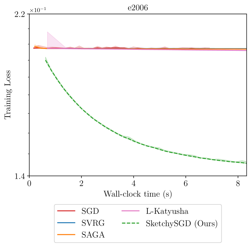
Figure 1: SketchySGD outperforms standard stochastic gradient optimizers, even when their parameters are tuned for optimal performance. Each optimizer was allowed 40 full data passes.

Second-order optimizers based on the Hessian, such as Newton’s method and quasi-Newton methods, are the classic remedy for ill-conditioning. These methods converge at super-linear rates under mild assumptions and are faster than first-order methods both in theory and in practice [38, 7]. Alas, it has proved difficult to design second-order methods that can use stochastic gradients. This deficiency limits their use in large-scale machine learning. Stochastic second-order methods using stochastic Hessian approximations — but full gradients — are abundant in the literature [42, 27, 47]. However, a practical second-order stochastic optimizer must replace both the Hessian and gradient by stochastic approximations. While many interesting ideas have been proposed, existing methods require impractical conditions for convergence: for example, a batch size for the gradient and Hessian that grows with the condition number [46], or that increases geometrically at each iteration [5]. These theoretical conditions are impossible to implement in practice. Convergence results without extremely large or growing batch sizes have been established under interpolation, i.e., if the loss is zero at the solution [34]. This setting is interesting for deep learning, but is unrealistic for convex machine learning models. Moreover, most of these methods lack practical guidelines for hyperparameter selection, making them difficult to deploy in real-world machine learning pipelines. Altogether, the literature does not present any stochastic second-order method that can function as a drop-in replacement for SGD, despite strong empirical evidence that — for perfectly chosen parameters — they yield improved performance. One major contribution of this paper is a theory that matches how these methods are used in practice, and therefore is able to offer practical parameter selection rules that make SketchySGD (and even some previously proposed methods) practical. We provide a more detailed discussion of how SketchySGD compares to prior stochastic second-order optimizers in Section 3.

SketchySGD accesses second-order information using only minibatch Hessian-vector products to form a sketch, and produces a preconditioner for SGD using the sketch, which is updated only rarely (every epoch or two). This primitive is perfectly compatible with the practice in modern large-scale machine learning, as it can be computed by automatic differentiation. Our major contribution is a tighter theory that enables practical choices of parameters that makes SketchySGD a drop-in replacement for SGD and variants that works out-of-the-box, without tuning, across a wide variety of problem instances.

How? A standard theoretical argument in convex optimization shows that the learning rate in a gradient method should be set as the inverse of the smoothness parameter of a function to guarantee convergence. This choice generally results in a tiny stepsize and very slow convergence. However, in the context of SketchySGD, the preconditioned smoothness constant is generally around $1$, and so its inverse provides a reasonable learning rate. Moreover, it is easy to estimate, again using minibatch Hessian-vector products to measure the largest eigenvalue of a preconditioned minibatch Hessian.

Theoretically, we establish SketchySGD converges linearly to a small ball around the optimum on smooth and strongly convex functions, which suffices for good test error [2, 21, 29]. By appealing to the modern theory of SGD for finite-sum optimization [18] in our analysis, we avoid vacuous or increasing batchsize requirements for the gradient. As a corollary of our theory, we obtain that SketchySGD converges linearly to the optimum whenever the model interpolates the data, recovering the result of [34]. In addition, we show that SketchySGD’s required number of iterations to converge, improves upon that of SGD by a factor of $O(\sqrt{n})$ in the setting of ill-conditioned ridge regression.

Numerical experiments verify that SketchySGD yields comparable or superior performance to SGD, SAGA, SVRG, stochastic L-BFGS [35], and loopless Katyusha [25] equipped with tuned hyperparameters that attain their best performance. Experiments also demonstrate that SketchySGD’s default hyperparameters, including the rank of the preconditioner and the frequency at which it is updated, work well across a wide range of datasets.

1.1 SketchySGD

Algorithm 1 SketchySGD

  Input: initialization $w_{0}$, hvp oracle $\mathcal{O}_{H}$, ranks $\{r_{j}\}$, regularization $\rho$, preconditioner update frequency $u$, stochastic Hessian batch sizes $\{b_{h_{j}}\}$

  repeat

     Sample a batch $B_{k}$

     Compute stochastic gradient $g_{B_{k}}(w_{k})$

     if $k\equiv 0\pmod{u}$ then

        Set $j=j+1$

        Sample a batch $S_{j}$ {$|S_{j}|=b_{h_{j}}$}

        $\Phi=\text{randn}(p,r_{j})$ {Gaussian test matrix}

        $Q=$ qr_econ $(\Phi)$

        Compute sketch $Y=H_{S_{j}}(w_{k})Q$ {$r$ calls to $\mathcal{O}_{H_{S_{j}}}$}

        $[\hat{V},\hat{\Lambda}]=$ RandNysApprox$(Y,Q,r_{j})$

        $\eta_{j}=\texttt{get\_learning\_rate}(\mathcal{O}_{H_{S_{j}}},\hat{V},\hat{\Lambda},\rho)$

     end if

     Compute $v_{k}=(\hat{H}_{S_{j}}+\rho I)^{-1}g_{B_{k}}(w_{k})$ via (4)

     $w_{k+1}=w_{k}-\eta_{j}v_{k}$ {Update parameters}

  until convergence

SketchySGD finds $w\in\mathbb{R}^{p}$ to minimize the convex empirical risk

(1) $$\mbox{minimize}\quad f(w):=\frac{1}{n}\sum_{i=1}^{n}f_{i}(w),$$

given access to a gradient oracle for each $f_{i}$. SketchySGD is formally presented as Algorithm 1. SketchySGD tracks two different sets of indices: $k$, which counts the number of total iterations, and $j$, which counts the number of (less frequent) preconditioner updates. SketchySGD updates the preconditioner (every $u$ iterations) by sampling a minibatch $S_{j}$ and forming a low-rank $\hat{H}_{S_{j}}$ using Hessian vector products with the minibatch Hessian $H_{S_{j}}$ evaluated at the current iterate $w_{k}$. Given the Hessian approximation, it uses $\hat{H}_{S_{j}}+\rho I$ as a preconditioner, where $\rho>0$ is a regularization parameter. Subsequent iterates are then computed as

(2) $$w_{k+1}=w_{k}-\eta_{j}(\hat{H}_{S_{j}}+\rho I)^{-1}g_{B_{k}}(w_{k}),$$

where $g_{B_{k}}(w_{k})$ is the minibatch stochastic gradient and $\eta_{j}$ is the learning rate, which is automatically determined by the algorithm.

The SketchySGD update may be interpreted as a preconditioned stochastic gradient step with Levenberg-Marquardt regularization [28, 30]. Indeed, let $P_{j}=\hat{H}_{S_{j}}+\rho I$ and define the preconditioned function $f_{P_{j}}(z)=f(P^{-1/2}_{j}z)$, which represents $f$ as a function of the preconditioned variable $z\in\mathbb{R}^{p}$. Then (2) is equivalent to

$$z_{k+1}=z_{k}-\eta_{j}\hat{g}_{P_{j}}(z_{k}),\quad w_{k+1}=P_{j}^{-1/2}z_{k},$$

where $\hat{g}_{P_{j}}(z_{k})$ is the minibatch stochastic gradient as a function of $z$. Thus, SketchySGD first takes a step of SGD in preconditioned space and then maps back to the original space. As preconditioning induces more favorable geometry, SketchySGD chooses better search directions and uses a stepsize adapted to the (more isotropic) preconditioned curvature. Hence SketchySGD makes more progress than SGD to ultimately converge faster.

Contributions

1. We develop a new robust stochastic quasi-Newton algorithm that is fast and generalizes well by accessing only a subsampled Hessian and stochastic gradient.

2. We devise an automated step size for this algorithm that works well in both ridge and logistic regression. More broadly, we present default settings for all hyperparameters of SketchySGD, which allow it to work out-of-the-box.

3. We show that SketchySGD converges linearly to a small ball around the optimum. Additionally, we show SketchySGD converges at a faster rate than SGD for ill-conditioned least-squares problems. We verify this improved convergence in numerical experiments.

4. We present experiments showing that SketchySGD with its default hyperparameters can match or outperform SGD, SVRG, SAGA, stochastic L-BFGS, and loopless Katyusha on ridge and logistic regression problems.

1.2 Roadmap

Section 2 describes the SketchySGD algorithm in detail, explaining how to compute $\hat{H}_{S_{k}}$ and the update in (2) efficiently. Section 3 surveys previous work on stochastic quasi-Newton methods, particularly in the context of machine learning. Section 4 establishes convergence of SketchySGD in convex machine learning problems. Section 5 provides numerical experiments showing the superiority of SketchySGD relative to competing optimizers.

1.3 Notation

Throughout the paper $B_{k}$ and $S_{j}$ denote subsets of $\{1,\ldots,n\}$ that are sampled independently and uniformly without replacement. The corresponding stochastic gradient and minibatch Hessian are given by

$$g_{B_{k}}(w)=\frac{1}{b_{g_{k}}}\sum_{i\in B_{k}}g_{i}(w),\quad H_{S_{j}}(w)=\frac{1}{b_{h_{j}}}\sum_{i\in S_{j}}\nabla^{2}f_{i}(w),$$

where $b_{g_{k}}=|B_{k}|,b_{h_{j}}=|S_{j}|.$ For shorthand we often omit the dependence upon $w$ and simply write $g_{B_{k}}$ and $H_{S_{j}}$. We also define $H(w)$ as the Hessian of the objective $f$ at $w$, and we set $M(w)=\max_{1\leq i\leq n}\|\nabla^{2}f_{i}(w)\|$. Similarly, for the gradient we set $G(w)=\max_{1\leq i\leq n}\|\nabla f_{i}(w)\|.$ Given any $\beta>0$, we use the notation $H^{\beta}_{S_{j}}$ to denote $H_{S_{j}}+\beta I$. We abbreviate positive-semidefinite as psd. We denote the Loewner order on the convex cone of psd matrices by $\preceq$, where $A\preceq B$ means $B-A$ is psd. Given a psd matrix $A\in\mathbb{R}^{p\times p}$, we enumerate its eigenvalues in descending order, $\lambda_{1}(A)\geq\lambda_{2}(A)\geq\cdots\geq\lambda_{p}(A)$. Finally given a psd matrix $A$ and $\beta>0$ we define the effective dimension by $d_{\textrm{eff}}(\beta)=\textrm{tr}(A(A+\beta I)^{-1})$, which provides a smoothed measure of the eigenvalues greater than or equal to $\beta$.

2 SketchySGD: efficient implementation and hyperparameter selection

We now formally describe SketchySGD (Algorithm 1) and its efficient implementation.

Hessian vector product oracle

SketchySGD relies on one main computational primitive, a (minibatch) Hessian vector product (hvp) oracle, to compute a low-rank approximation of the (minibatch) Hessian. Access to such an oracle naturally arises in machine learning problems. In the case of generalized linear models (GLMs), the Hessian is given by $H(w)=\frac{1}{n}A^{T}D(w)A$, where $A\in\mathbb{R}^{n\times p}$ is the data matrix and $D\in\mathbb{R}^{n\times n}$ is a diagonal matrix. Accordingly, an hvp between $H_{S_{j}}(w)$ and $v\in\mathbb{R}^{p}$ is given by

$$H_{S_{j}}(w)v=\frac{1}{b_{h_{j}}}\sum_{i\in S_{j}}d_{i}(w)a_{i}\left(a_{i}^{T}v\right).$$

For more complicated losses, an hvp can be computed by automatic differentiation (AD) [39]. The general cost of $r$ hvps with $H_{S_{j}}(w)$ is $O(b_{h_{j}}pr)$. In contrast, explicitly instantiating a Hessian entails a heavy $O(p^{2})$ storage and $O(np^{2})$ computational cost. Further computational gains can be made when the subsampled Hessian enjoys more structure, such as sparsity. If $H_{S_{j}}(w)$ has $s$-sparse rows then the complexity of $r$ hvps enjoys a significant reduction from $O(b_{h_{j}}pr)$ to $O(b_{h_{j}}sr)$. Hence, computing hvps with $H_{S_{j}}(w)$ is extremely cheap in the sparse setting.

Randomized low-rank approximation

The hvp primitive allows for efficient randomized low-rank approximation to the minibatch Hessian by sketching. Sketching reduces the cost of fundamental numerical linear algebra operations without much loss in accuracy [53, 31] by computing the quantity of interest from a sketch, or randomized linear image, of a matrix. In particular, sketching enables efficient computation of a near-optimal low-rank approximation to $H_{S_{j}}$ [20, 11, 51].

SketchySGD computes a sketch of the subsampled Hessian using hvps and returns a randomized low-rank approximation $\hat{H}_{S_{j}}$ of $H_{S_{j}}$ in the form of an eigendecomposition $\hat{V}\hat{\Lambda}\hat{V}^{T}$, where $\hat{V}\in\mathbb{R}^{p\times r}$ and $\hat{\Lambda}\in\mathbb{R}^{r\times r}$. In this paper, we use the randomized Nyström approximation, following the stable implementation in [50]. The resulting algorithm RandNysApprox appears in Appendix A. The cost of forming the Nyström approximation is $O(b_{h_{j}}pr+pr^{2})$, as we need to perform $r$ minibatch hvps to compute the sketch, and we must perform a skinny SVD at a cost of $O(pr^{2})$. The procedure is extremely cheap, as we find empirically we can take $r$ to be $10$ or less, so constructing the low-rank approximation has negligible cost.

Remark 2.1.

If the objective for $f$ includes an $l_{2}$-regularizer $\gamma$, so that the subsampled Hessian has the form $H_{S_{j}}(w)=\frac{1}{b_{h_{j}}}\sum_{i\in S_{j}}\nabla^{2}f_{i}(w)+\gamma I$, we do not include $\gamma$ in the computation of the sketch in Algorithm 1. The sketch is only computed using minibatch hvps with $\frac{1}{b_{h_{j}}}\sum_{i\in S_{j}}\nabla^{2}f_{i}(w)$.

Setting the learning rate

Significantly, SketchySGD automatically selects the learning rate $\eta$ whenever it updates the preconditioner. SketchySGD sets the learning rate as

(3) $$\eta_{\textrm{SketchySGD}}=\frac{1}{2\lambda_{1}\left((\hat{H}_{S_{j}}+\rho I)^{-1/2}H_{S^{\prime}}(\hat{H}_{S_{j}}+\rho I)^{-1/2}\right)},$$

where $S^{\prime}$ is a fresh minibatch that is sampled independently of $S_{j}$. The intuition behind this choice is that this quantity should closely mimic the reciprocal of the preconditioned smoothness constant. Hence, it should give a good step-size. The learning rate can be efficiently computed via matvecs with $H_{S_{j}}$ and $(\hat{H}_{S_{j}}+\rho I)^{-1/2}$ using techniques from randomized linear algebra, such as randomized powering and the randomized Lanczos method [26, 31]. Observe for any vector $v$, $(\hat{H}_{S_{j}}+\rho I)^{-1/2}v$ may be straightforwardly computed given (4) below. As an example we show how the learning rate may be computed by using randomized powering in Algorithm 2.

Algorithm 2 get_learning_rate

  Input: hvp oracle $\mathcal{O}_{H}$, Nyström approximation factors $\hat{V},\hat{\Lambda}$, regularization $\rho$, maximum number of iterations $q$

  $z$ = randn$(p,1)$

  $y_{0}=z/\|z\|$

  for $i=1,\dots,q$ do

     Compute $v=\left(\hat{H}_{S_{j}}+\rho I\right)^{-1/2}y_{i-1}$ {Use (4)}

     Compute $v^{\prime}=H_{S^{\prime}}u$ by calling oracle $\mathcal{O}_{H_{S_{k}}}$

     Compute $y_{i}=\left(\hat{H}_{S_{j}}+\rho I\right)^{-1/2}v^{\prime}$ {Use (4)}

     $\lambda_{i}=y_{i-1}^{T}y_{i}$

     $y_{i}=y_{i}/\|y_{i}\|$

  end for

  Set $\eta=1/\lambda_{q}$

  Return: $\eta$

Computing the SketchySGD update (2) fast

Given the rank-$r$ approximation $\hat{H}_{S_{j}}=\hat{V}\hat{\Lambda}\hat{V}^{\top}$ to the minibatch Hessian $H_{S_{j}}$, the main cost of SketchySGD relative to standard SGD is computing the search direction $v_{k}=(\hat{H}_{S_{j}}+\rho I)^{-1}g_{B_{k}}$. This (parallelizable) computation requires $O(pr)$ flops, by the Woodbury formula [22]:

(4) $$v_{k}=\hat{V}\left(\hat{\Lambda}+\rho I\right)^{-1}\hat{V}^{T}g_{B_{k}}+\frac{1}{\rho}(g_{B_{k}}-\hat{V}\hat{V}^{T}g_{B_{k}}).$$

Thus, the cost of applying the SketchySGD preconditioner is extremely cheap, and enables the method to scale to the massive problem instances that frequently arise in contemporary machine learning.

Default parameters for Algorithm 1

We recommend setting the ranks $\{r_{j}\}$ to a constant value of $10$, the regularization $\rho=10^{-3}$, and the stochastic Hessian batch sizes $\{b_{h_{j}}\}$ to a constant value of $\left\lfloor\sqrt{n_{\mathrm{tr}}}\right\rfloor$, where $n_{\mathrm{tr}}$ is the size of the training set. When the Hessian is constant, i.e. as in least-squares/ridge-regression, we recommend using the preconditioner throughout the optimization, which corresponds to $u=\infty$. In settings where the Hessian is not constant, we recommend setting $u=\left\lceil\frac{n_{\textrm{tr}}}{b_{g}}\right\rceil$, which corresponds to updating the preconditioner after each pass through the training set.

3 Comparison to previous work

Many authors have developed stochastic quasi-Newton methods for large-scale machine learning. Broadly, these schemes can be grouped by whether they use a stochastic approximations to the Hessian and the gradient or just a stochastic approximation to the Hessian. Stochastic quasi-Newton methods that use exact gradients with a stochastic Hessian approximation constructed via sketching or subsampling include [8, 14, 42, 17, 55]. Methods falling into the second group include [35, 6, 46, 5, 34].

Arguably, the most common strategy employed by stochastic quasi-Newton methods is to subsample the Hessian as well as the gradient. These methods either directly apply the inverse of the subsampled Hessian to the stochastic gradient [46, 5, 34], or they do an L-BFGS-style update step with the subsampled Hessian [35, 6, 34]. However, the theory underlying these methods is unsatisfactory, requiring large or growing gradient batch sizes [46, 6, 5], periodic full gradient computation [35], or interpolation [34]. Further, these methods lack practical guidelines for setting hyperparameters such as batch sizes and learning rate, leading to the same tuning issues that plague stochastic first-order methods.

SketchySGD improves on these stochastic quasi-Newton methods by providing principled guidelines for selecting hyperparameters and requiring only a modest, constant batch size. Table 1 shows that SketchySGD compares favorably to a representative subset of stochastic second-order methods with respect to required batch sizes for the gradient and the Hessian. Notice that SketchySGD is the only method that allows computing the gradient with a small constant batch size! Hence SketchySGD empowers the user to select the gradient batch size that meets their computational constraints.

SketchySGD also generalizes subsampled Newton methods; by letting the rank parameter $r_{j}\to\mathrm{rank}(H_{S_{j}})\leq p$, SketchySGD reproduces the algorithm of [46, 5, 34]. By using a full batch gradient $b_{g}=n$ (and a regularized exact low-rank approximation to the subsampled Hessian), SketchySGD reproduces the method of [14]. In particular, these methods are made practical by the analysis and practical parameter selections in this work.

Table 1: Comparison of stochastic 2nd-order methods. The table compares the required gradient and Hessian batch sizes of various stochastic quasi-Newton methods. Here $\varepsilon\in(0,1)$, while $G(w)$ and $M(w)$ are as in Section 1.3, and $\tau_{\rho}(H(w))$ denotes the $\rho$-similarity, which is defined in Definition 4.3. The $\rho$-similarity offers the tightest characterization of the required Hessian minibatch size required to ensure a non-trivial approximation of $H^{\rho}$. In many settings of interest, the $\rho$-similarity satisfies $\tau_{\rho}(H(w))=\tilde{O}(\sqrt{n})$, so it is much smaller than $n.$

method	gradient batch size	Hessian batch size	Source
Newton Sketch	Full	Full	[42, 27]
Subsampled Newton	$\widetilde{O}\left(\frac{G(w)}{\varepsilon^{2}}\right)$	$\widetilde{O}\left(\frac{M(w)}{\mu}\right)$	[46, 55]
Subsampled Newton+Low-rank	Full	$\widetilde{O}\left(\frac{M(w)}{\lambda_{r+1}(H(w))}\right)$	[14, 55]
SLBFGS	Full eval every epoch	$b_{h}$	[35]
SketchySGD	$b_{g}$	$\widetilde{O}\left(\tau_{\rho}(H(w))\right)$	This paper

4 Theory

In this section we give our main convergence theorem for SketchySGD (Algorithm 1). For the analysis, we shall assume that the preconditioner is updated every iteration, i.e. $u=1$ and $j=k$. Empirically SketchySGD does not require such frequent updates to succeed, furthermore frequent updating does not always lead to better performance, see Section 5.4.2 for details. Extending the analysis given here to the infrequent update setting provides an excellent direction for future work.

4.1 Assumptions

We now prove convergence of SketchySGD when $f$ is smooth and strongly convex, as formally elucidated by Section 4.1 and Section 4.1.

[Differentiability and smoothness] The function $f$ is twice differentiable and $L$-smooth. Further, each $f_{i}$ is $L_{i}$-smooth with $L_{i}\leq L_{\textup{max}}$ for every $i=1,\ldots,n$.

[Strong convexity] The function $f$ is $\mu$-strongly convex for some $\mu>0$.

4.2 Relative-smoothness and relative-convexity

Our analysis of the convex case requires the notions of relative smoothness and relative convexity from [17].

Definition 4.1 (Relative smoothness and relative convexity).

Let $f$ be a twice differentiable function. Then the relative smoothness constant is defined by

(5) $$\hat{L}\coloneqq\sup_{w,w^{\prime}\in\mathbb{R}^{p}}\int_{0}^{1}2(1-t)\frac{\|w^{\prime}-w\|^{2}_{H(w+t(w^{\prime}-w))}}{\|w^{\prime}-w\|^{2}_{H(w)}}dt.$$

Similarly, the relative convexity constant is defined by

(6) $$\hat{\mu}\coloneqq\inf_{w,w^{\prime}\in\mathbb{R}^{p}}\int_{0}^{1}2(1-t)\frac{\|w^{\prime}-w\|^{2}_{H(w+t(w^{\prime}-w))}}{\|w^{\prime}-w\|^{2}_{H(w)}}dt.$$

We say $f$ is relatively smooth (relatively convex) if $\hat{L}<\infty$ ($\hat{\mu}>0$).

The following result easily follows from Definition 4.1, see [17].

Proposition 4.2 (relative-smoothness bounds).

Let $f$ be relatively smooth and relatively convex. Then for all $w,w^{\prime}\in\mathbb{R}^{p}$, the following inequalities hold:

(7) $$f(w^{\prime})\leq f(w)+\langle g(w),w^{\prime}-w\rangle+\frac{\hat{L}}{2}\|w^{\prime}-w\|^{2}_{H(w)},$$

(8) $$f(w^{\prime})\geq f(w)+\langle g(w),w^{\prime}-w\rangle+\frac{\hat{\mu}}{2}\|w^{\prime}-w\|^{2}_{H(w)}.$$

Relative smoothness and relative convexity were introduced in [17]. These assumptions are weaker than assuming $f$ is $L$-smooth and $\mu$-strongly convex. Indeed, it is easy to show that if $f$ is $L$-smooth and $\mu$-strongly convex then $f$ is relatively smooth and relatively convex, see [17] for details. More importantly, (7) and (8) hold with non-vacuous values of $\hat{L}$ and $\hat{\mu}$. In the case of least-squares $\hat{L}=\hat{\mu}=1$, and for generalized linear models $\hat{L}$ and $\hat{\mu}$ are independent of the condition number $\kappa=L/\mu$ [17]. Thus, for many popular machine learning problems the relative condition number $\hat{\kappa}=\hat{L}/\hat{\mu}$ is independent of the conditioning of the data.

4.3 Quality of SketchySGD preconditioner

To control the batch size used to form the subsampled Hessian, we introduce $\rho$-similarity.

Definition 4.3 ($\rho$-similarity).

Let $H(w)$ be the Hessian at $w$, then the $\rho$-similarity is given by

$$\tau_{\rho}(H(w))=\max_{1\leq i\leq n}\lambda_{1}\left((H+\rho I)^{-1/2}(\nabla^{2}f_{i}(w)+\rho I)(H+\rho I)^{-1/2}\right).$$

$\rho$-Similarity may be viewed as an analogue of coherence from compressed sensing and low-rank matrix completion [10, 9]. Similar to how the coherence parameter measures the uniformity of a matrix’s rows, $\tau_{\rho}(H(w))$ measures how uniform the curvature of the sample $\{\nabla^{2}f_{i}(w)\}_{1\leq i\leq n}$ is. Intuitively, the more uniform the curvature, the better the sample average $H(w)$ captures the curvature of each individual Hessian, which corresponds to smaller $\tau_{\rho}(H(w))$. On the other hand if the curvature is highly non-uniform, curvature information of certain individual Hessians will get diluted by the averaging in $H(w)$, which leads to a large value of $\tau_{\rho}(H(w))$.

The following lemma provides an upper bound on the $\rho$-similarity. In particular, it shows that the $\rho$-similarity never exceeds $n$. The proof may be found in Section B.2.

Lemma 4.4 ($\rho$-Similarity never exceeds $n$).

For any $\rho\geq 0$ and $w\in\mathbb{R}^{p}$, the following inequality holds

$$\tau_{\rho}(H(w))\leq\min\left\{n,\frac{M(w)+\rho}{\mu+\rho}\right\},$$

where $M(w)=\max_{1\leq i\leq n}\lambda_{1}(\nabla^{2}f_{i}(w)).$

Lemma 4.4 yields two interesting implications. First, if the curvature of the sample is highly non-uniform then the $\rho$-similarity can be large as $n$. Second, the $\rho$-similarity approaches $1$ as $\rho$ becomes larger, which is intuitive. Once $\rho$ is large enough it dominates the individual Hessians. However by itself Lemma 4.4 is not very encouraging, as we hope $\tau_{\rho}(H(w))\ll n$, but the local condition number $(M(w)+\rho)/(\mu+\rho)$ could easily be on the order of $n$. Nevertheless, Lemma 4.4 is worst-case in nature, and fails to account for the possibility the $f_{i}$’s maybe very similar in many practical settings. When the $f_{i}$’s enjoy some similarity, $\tau_{\rho}(H(w))$ ought to be much smaller than the the bound given in Lemma 4.4. Fortunately, machine learning problems naturally provide such a setting, as we discuss next.

We now argue in common machine learning settings that $\tau_{\rho}(H(w))$ is much smaller than $n$. This result is natural when we recall each $f_{i}$ corresponds to the loss of some model on a datapoint $z_{i}$, that is $f_{i}(w)=\ell(z_{i};w)$, where $\ell$ is the loss function. As the data is typically i.i.d. from some unknown distribution, it is natural to expect some similarity between the individual Hessians. In past analyses of empirical risk minimization, this similarity has been encoded by making distributional or moment assumptions on the random variable $\ell(z;w)$ or its derivatives [54, 32, 41].

Inspired by these prior works, in the following proposition we assume $\nabla^{2}\ell(z;w)$ is a $\nu^{2}$-sub-Gaussian random matrix The proof of this proposition is provided in Section B.3, along with the formal definition of a $\nu^{2}$-sub-Gaussian random matrix.

Proposition 4.5 ($\rho$-similarity is well-behaved in the machine learning setting).

Let $\ell(z;w):\mathbb{R}^{p}\times\mathbb{R}^{p}\mapsto\mathbb{R}$ be smooth and convex in its second argument. Suppose that $f$ is as in (1), with $f_{i}(w)=\ell(z_{i};w)$, where $z_{i}$ is generated $i.i.d.$ from some unknown distribution ${\mathbb{P}}(z)$. Fix $\delta\in(0,1)$. Then if $\nabla^{2}\ell(z;w)$ is $\nu^{2}$-sub-Gaussian for each $w\in\mathbb{R}^{p}$ and $\rho\geq 1/\sqrt{n}$,

$$\tau_{\rho}(H(w))\leq 1+\sqrt{{8\nu^{2}n\log\left(\frac{2np}{\delta}\right)}},$$

with probability at least $1-\delta$.

Proposition 4.5 shows when $\nabla^{2}f(z;w)$ is sub-Gaussian, with high probability $\tau_{\rho}(H(w))=\widetilde{O}\left(\sqrt{n}\right)$. Hence when statistical similarity is accounted for, the $\rho$-similarity $\tau_{\rho}(H(w))$ is much smaller than the pessimistic upper bounds in Lemma 4.4. We note that if the covariance matrix is sub-Gaussian, and $\ell(z;w)=\ell(z^{T}w)$, then $\nabla^{2}\ell(z;w)$ is sub-Gaussian if $\ell^{\prime\prime}$ is bounded. Thus, Proposition 4.5 applies to least-squares and logistic regression whenever the covariance matrix is sub-Gaussian. So in many practical settings of interest, $\tau_{\rho}(H(w))$ is far smaller than $n$ for a wide range of values of $\rho$.

The following lemma makes rigorous, the claim that the $\rho$-similarity controls the required batch size for the minibatch Hessian. The proof of the lemma is provided in Section B.4.

Lemma 4.6 (Closeness in Loewner ordering between $H^{\rho}_{S}(w)$ and $H^{\rho}(w)$).

Let $\zeta\in(0,1)$, $w\in\mathbb{R}^{p}$ , and $\rho\geq 0$. Suppose we construct $H_{S}$ with batch size $b_{h}=O\left(\frac{\tau_{\rho}(H(w))\log(\frac{p}{\delta})}{\zeta^{2}}\right)$. Then with probability at least $1-\delta$

$$(1-\zeta)H^{\rho}_{S}(w)\preceq H^{\rho}(w)\preceq(1+\zeta)H^{\rho}_{S}(w).$$

Lemma 4.6 refines prior analysis such as [55], where $b_{h}$ depends upon the local-condition number $(M(w)+\rho)/(\mu+\rho)$, which Lemma 4.4 shows is always larger than $\tau_{\rho}(H(w))$. Hence the dependence upon $\tau_{\rho}(H(w))$ in Lemma 4.6 leads to a tighter bound on the required Hessian batch size. Further Proposition 4.5 shows that $\tau_{\rho}(H(w))=\tilde{O}(\sqrt{n})$, which is far smaller then $n$, hence we can get a good approximation to Hessian with a non-vacuous batch size. Motivated by the previous observation, we recommend a default batch size of $b_{h}=\sqrt{n_{\textrm{tr}}}$, which leads to excellent performance in practice, see Section 5 for numerical evidence.

Utilizing our results on subsampling and ideas from randomized low-rank approximation, we are able to establish the following result, which quantifies how the SketchySGD preconditioner reduces the condition number. The proof of this proposition is given in Section B.5.

Proposition 4.7 (Closeness in Loewner ordering between $H_{k}$ and $\hat{H}_{S_{k}}^{\rho}$).

Let $\zeta\in$$(0,1)$. Suppose at iteration $k$ we construct $H_{S_{k}}$ with batch size $b_{h_{k}}=O\left(\frac{\tau_{\rho}(H(w_{k}))\log(\frac{p}{\delta})}{\zeta^{2}}\right)$ and SketchySGD uses a low-rank approximation $\hat{H}_{S_{k}}$ to $H_{S_{k}}$ with rank $r_{k}=O(d_{\textup{eff}}(\zeta\rho)+\log(\frac{1}{\delta}))$. Then with probability at least $1-\delta$,

(9) $$(1-\zeta)\frac{\mu}{\mu+\rho}\hat{H}_{S_{k}}^{\rho}\preceq H_{k}\preceq(1+\zeta)\hat{H}^{\rho}_{S_{k}}.$$

Proposition 4.7 shows that with high probability, the SketchySGD preconditioner reduces the conditioner number from $L/\mu$ to $(1+\rho/\mu)$, which yields an $L/\rho$ improvement over the original value. The proposition also reveals a natural trade-off between eliminating dependence upon $\mu$ and the size of $b_{h}$. We could set $\rho$ to be $\mu$, which would make the preconditioned condition number equal to $2$ with high probability, but this would come at the cost of increasing $b_{h}$. Conversely, we can increase $\rho$ to reduce $b_{h}$, but this leads to a larger preconditioned condition number. In practice, we have found that a fixed-value of $\rho=10^{-3}$ yields excellent performance. Numerical results showing how the SketchySGD preconditioner improves the conditioning of the Hessian throughout the optimization trajectory are presented in Appendix D.

The other thing of note about Proposition 4.7 is that requires it requires the rank of $\hat{H}_{S_{k}}$ to satisfy $r_{k}=\tilde{O}\left(d_{\textrm{eff}}(\zeta\rho)\right)$, which corresponds to the rank such that $\|\hat{H}_{S_{k}}-H_{S_{k}}\|\leq\zeta\rho$ holds with high probability (see Lemma B.9). This rank requirement is intuitive, as the directions associated with eigenvalues smaller than $\rho$ get eliminated due to regularization. Therefore these directions can be thrown away, which is precisely what SketchySGD does by working with a low-rank approximation to the subsampled Hessian. In practice we set $r=10$, empirically we verify that SketchySGD is not very sensitive to this choice, see Section 5.4.1 for details.

We also have the following corollary, which follows from a straightforward union bound argument.

Corollary 4.8 (Union bound).

Let $\mathcal{E}_{T}=\bigcap_{k=0}^{T-1}\mathcal{E}_{k}$, where

$$\mathcal{E}_{k}=\left\{(1-\zeta)\frac{\mu}{\mu+\rho}\hat{H}_{S_{k}}^{\rho}\preceq H_{k}\preceq(1+\zeta)\hat{H}^{\rho}_{S_{k}}\right\},$$

and suppose that at iteration $k$ we construct $\hat{H}_{S_{k}}$ with rank $r_{k}=O\left(d_{\textup{eff}}(\zeta\rho)+\log\left(\frac{T}{\delta}\right)\right)$. Then

$${\mathbb{P}}(\mathcal{E}_{T})\geq 1-\delta.$$

4.4 Controlling the variance of the preconditioned stochastic gradient

A key component of establishing convergence of SketchySGD is to control the variance of the preconditioned minibatch stochastic gradient. The first step in achieving this aim, is the following technical result, which shows the preconditioned smoothness constants are uniformly bounded with probability $1$. The proof of the lemma is provided in Section B.7.

Lemma 4.9 (Preconditioned smoothness bounds).

Let $P_{k}=\hat{H}_{S_{k}}^{\rho}$. Instate the the hypotheses of Section 4.1 and Section 4.1. Consider the random variables

$$X_{P_{k_{i}}}=\sup_{k\geq 0}\left(\sup_{w\in\mathbb{R}^{p}}\lambda_{1}\left(P_{k}^{-1/2}\nabla^{2}f_{i}(w)P_{k}^{-1/2}\right)\right),\quad i\in\{1,\cdots,n\}.$$

Given $i\in\{1,\cdots,n\}$, define $L_{P_{i}}$ to be the smallest $C$ such that

$$X_{P_{k_{i}}}\leq C\quad\text{with probability 1}.$$

Similarly, define $L_{P_{\textup{max}}}$ to be the smallest $C$ such that for all $i\in\{1,\cdots,n\}$

$$X_{P_{k_{i}}}\leq C\quad\text{with probability 1}.$$

Then $L_{P_{\textup{max}}}$ and each $L_{P_{i}}$ are finite.

Our next result directly bounds the variance of the preconditioned stochastic gradient, and builds upon the expected smoothness analysis from [18]. The proof of this proposition may be found in Section B.8.

Proposition 4.10 (Preconditioned expected smoothness and gradient variance).

Let $P_{k}=\hat{H}_{S_{k}}^{\rho}$. Instate Section 4.1 and Section 4.1. Then for any iteration $k$, the following inequalities hold:

$$\mathbb{E}_{k}\|g_{B_{k}}(w_{k})-g_{B_{k}}(w_{\star})\|_{P^{-1}_{k}}^{2}\leq 2\mathcal{L}_{P}\left(f(w_{k})-f(w_{\star})\right),$$

$$\mathbb{E}_{k}\|g_{B_{k}}(w_{k})\|_{P^{-1}_{k}}^{2}\leq 4\mathcal{L}_{P}\left(f(w_{k})-f(w_{\star})\right)+\frac{2\sigma^{2}}{\rho}.$$

Where $\mathcal{L}_{P}$ and $\sigma^{2}$ satisfy:

$$\mathcal{L}_{P}\leq\left[\frac{n(b_{g}-1)}{b_{g}(n-1)}\frac{1}{n}\sum_{i=1}^{n}L_{P_{i}}+\frac{n-b_{g}}{b_{g}(n-1)}L_{P_{\textup{max}}}\right],\quad\sigma^{2}\coloneqq\frac{n-b_{g}}{b_{g}(n-1)}\frac{1}{n}\sum_{i=1}^{n}\|\nabla f_{i}(w_{\star})\|^{2}.$$

As in [18], the bounds in Proposition 4.10 depend upon two quantities: $\mathcal{L}_{P}$ and $\sigma^{2}$. The second quantity is simply the variance of the stochastic gradient at the optimum. The first quantity $\mathcal{L}_{P}$, is the preconditioned analogue of the expected smoothness constant $\mathcal{L}$ from [18], and we refer to it as the preconditioned expected smoothness constant.

4.5 Convergence of SketchySGD

In the analysis, we shall require the following technical assumption. [Stable metric evolution] Consider the random variable

$$X_{T}=\prod^{T-1}_{k=1}\frac{\|w_{k}-w_{\star}\|_{P_{k}}^{2}}{\|w_{k}-w_{\star}\|_{P_{k-1}}^{2}},$$

where $T>0$. Then for all $T>0$, there exists a constant $\Xi>0$ such that

$$X_{T}\leq\Xi\quad\textup{with probability}\hskip 3.0pt1.$$

Section 4.5 states that the cumulative effect of the metric changing from $P_{k-1}$ to $P_{k}$ stays bounded over the run of the algorithm. Thus, the metric evolves stably in the sense that $\|w_{k}-w_{\star}\|_{P_{k}}^{2}$ does not blow-up relative to $\|w_{k}-w_{\star}\|^{2}_{P_{k-1}}$.

Last, we shall need the following lemma, which is a preconditioned analogue of the strong convexity lower bound from convex optimization. The proof may be found in Section B.6.

Lemma 4.11 (Preconditioned strong convexity bound).

Let $P_{k}=\hat{H}_{S_{k}}^{\rho}$. Assume the conclusion of Proposition 4.7 holds. Then

$$f(w_{\star})\geq f(w_{k})-\langle P_{k}^{-1}g_{k},w_{k}-w_{\star}\rangle_{P_{k}}+\frac{\hat{\mu}_{P}}{2}\|w_{k}-w_{\star}\|_{P_{k}}^{2},$$

where $\hat{\mu}_{P}=(1-\zeta)\frac{\mu\hat{\mu}}{\mu+\rho}$.

We now state the main convergence result for the SketchySGD algorithm.

Theorem 4.12 (SketchySGD convergence).

Instate Assumptions 4.1–4.5. Run Algorithm 1 for

$$T\geq\max\left\{\frac{2(1+\frac{\rho}{\mu})}{(1-\zeta)}\frac{\mathcal{L}_{P}}{\hat{\mu}},\frac{\rho}{\mu^{2}}\left(1+\frac{\mu}{\rho}\right)^{2}\left(\frac{2\sigma}{(1-\zeta)\hat{\mu}}\right)^{2}\frac{\Xi}{\epsilon}\right\}\log\left(\frac{2(1+\zeta)\Xi\|w_{0}-w_{\star}\|_{H(w_{0})}}{\epsilon}\right)$$

iterations with gradient batch size $b_{g}$, regularization $\min\{1,\mu\}\leq\rho\leq 1$, Hessian batch size $b_{h_{k}}=O\left(\frac{\tau_{\rho}(H(w_{k}))}{\zeta^{2}}\log(\frac{p}{\delta})\right)$, learning rate $\eta=\min\left\{\frac{1}{2\mathcal{L}_{P}},\frac{\mu}{(1-\zeta)(\mu+\rho)}\frac{\epsilon\rho\hat{\mu}}{4\sigma^{2}\Xi}\right\}$, and at each iteration construct the randomized Nyström approximation with rank $r_{k}=O(d_{\textup{eff}}(\zeta\rho)+\log\left(\frac{1}{\delta}\right))$. Then conditioned on the event in Corollary 4.8, we have that

$${\mathbb{E}}\left[\|w_{T}-w_{\star}\|_{P_{T-1}}^{2}\right]\leq\epsilon.$$

An immediate corollary of Theorem 4.12 is that SketchySGD converges linearly to the optimum when $\sigma^{2}=0$, which corresponds to the setting when the model interpolates the data.

Corollary 4.13 (Convergence under interpolation).

Suppose $\sigma^{2}=0$, and instate the hypotheses of Theorem 4.12. Then after $T\geq 2\frac{\left(1+\frac{\rho}{\mu}\right)}{1-\zeta}\frac{\mathcal{L}_{P}}{\hat{\mu}}\log\left(\frac{2(f(w_{0})-f(w_{\star}))}{\epsilon}\right)$ iterations, we have

$${\mathbb{E}}\left[\|w_{T}-w_{\star}\|_{P_{T-1}}^{2}\right]\leq\epsilon.$$

Discussion

Theorem 4.12 shows with appropriate fixed learning rate, SketchySGD converges to small-ball about the optimum. For sufficiently small $\epsilon$, SketchySGD reaches $\epsilon$-suboptimality in $O\left(\frac{\rho}{\mu^{2}}\frac{\sigma^{2}}{\hat{\mu}^{2}}\frac{\log\left(\frac{1}{\epsilon}\right)}{\epsilon}\right)$ iterations. In the case where each $f_{i}$ is quadratic, so that $\hat{L}=\hat{\mu}=1$, this simplifies to $O\left(\frac{\rho\sigma^{2}}{\mu^{2}}\frac{\log\left(\frac{1}{\epsilon}\right)}{\epsilon}\right)$. Meanwhile, it is known in the smooth and strongly-convex setting that SGD satisfies an upper-bound of $O\left(\frac{\sigma^{2}}{\mu^{2}}\frac{\log\left(\frac{1}{\epsilon}\right)}{\epsilon}\right)$ iterations [18, Theorem 3.1, p. 4]. Hence SketchySGD achieves an improvement ratio of $O(\frac{1}{\rho})$, which yields a significant gain in the ill-conditioned setting, as $\rho\ll 1$. To make this more concrete, we show below in Corollary 4.14 , that for ill-conditioned ridge regression, the improvement ratio is $O(\sqrt{n})$ for properly selected $\rho$. More broadly, similar improvement from SketchySGD is expected whenever $\hat{\mu}$ is well-behaved, such as when $f$ belongs to the family of GLMs. In Section 5 below, we verify these projected gains are realized in practice on real-world problems involving ridge regression and $l_{2}$–regularized logistic regression.

When interpolation holds, Corollary 4.13 shows that SketchySGD converges linearly to $\epsilon$-suboptimality in at most $O\left(\frac{\rho\mathcal{L}_{P}}{\mu\hat{\mu}}\log\left(\frac{1}{\epsilon}\right)\right)$ iterations. In the regime when $\frac{\mathcal{L}_{P}}{\hat{\mu}}$ satisfies $\frac{\mathcal{L}_{P}}{\hat{\mu}}=O(1)$, which corresponds to the setting where Hessian information can help, SketchySGD enjoys a convergence rate of $O\left(\frac{\rho}{\mu}\log\left(\frac{1}{\epsilon}\right)\right)$, faster than the $O\left(\kappa\log\left(\frac{1}{\epsilon}\right)\right)$ rate of gradient descent. This improves upon prior analyses that consider stochastic Newton methods in the interpolation setting, and fail to show the benefit of using Hessian information. For instance $\rho$-regularized subsampled-Newton, a special case of SketchySGD, was only shown to converge in at most $O\left(\frac{\kappa L}{\rho}\log\left(\frac{1}{\epsilon}\right)\right)$ iterations in [34, Theorem 1, p. 3]. Hence the latter result shows no benefit to using Hessian information, and is worse than the convergence rate of gradient descent by a factor of $O(L/\rho)$.

4.6 When does SketchySGD improve over SGD?

We now present a concrete setting illustrating when SketchySGD converges faster than SGD. We assume that each $f_{i}$ is the least-squares loss, so that the Hessian $H$ is constant. In practice we often have an $l_{2}$-regularizer $\gamma$, which is typically chosen as $\gamma=\frac{C}{n}$, for some constant $C>0$. The regularizer ensures that $\mu=O\left(\frac{1}{n}\right)$. The following corollary establishes SketchySGD’s iteration complexity in this setting, when $\epsilon$ is sufficiently small.

Corollary 4.14 (SketchySGD converges fast).

Instate the hypotheses of Theorem 4.12. Assume each $f_{i}$ is the least-squares loss, $\mu=\frac{C}{n}$, $\rho=\sqrt{n}\mu=\frac{C}{\sqrt{n}}$. Then if we run Algorithm 1 for

$$T\geq n^{3/2}\left(1+\frac{1}{\sqrt{n}}\right)^{2}\frac{4\sigma^{2}}{(1-\zeta)^{2}}\frac{\log\left(\frac{2(1+\zeta)\Xi\|w_{0}-w_{\star}\|_{H(w_{0})}}{\epsilon}\right)}{\epsilon}\quad\text{iterations,}$$

we have

$${\mathbb{E}}\left[\|w_{T}-w_{\star}\|^{2}_{P}\right]\leq\epsilon.$$

The preceding result shows SketchySGD yields an $\epsilon$-optimal point in $\tilde{O}\left(\frac{n^{3/2}\sigma^{2}}{\epsilon}\right)$ iterations. Conversely, SGD’s upper-bound yields $\tilde{O}\left(\frac{n^{2}\sigma^{2}}{\epsilon}\right)$ iterations in this setting. Hence for ill-conditioned ridge regression, SketchySGD exhibits a $O(\sqrt{n})$-improvement over SGD. The predictions of Corollary 4.14 carry over in practice, Section 5 shows SketchySGD outperforms tuned SGD on real ridge regression problems.

4.7 Proof of Theorem 4.12

We now turn to the proof of Theorem 4.12.

Proof 4.15.

To avoid notational clutter in the proof, we define the following quantities:

$$P_{k}\coloneqq\hat{H}_{S_{k}}^{\rho},\quad\hat{\mu}_{P}\coloneqq(1-\zeta)\frac{\mu\hat{\mu}}{\mu+\rho}.$$

With these notational preliminaries out the way, we now commence the proof.

Consider $\|w_{T}-w_{\star}\|_{P_{T}}^{2}$, expanding we have

$$\|w_{T}-w_{\star}\|_{P_{T-1}}^{2}=\|w_{T-1}-w_{\star}\|_{P_{T-1}}^{2}-2\eta\langle P_{T-1}^{-1}g_{B_{T-1}},w_{T-1}-w_{\star}\rangle_{P_{T-1}}+\eta^{2}\|g_{B_{T-1}}\|^{2}_{P_{T-1}^{-1}}.$$

Taking the expectation conditioned on $T-1$, we reach

$${\mathbb{E}}_{T-1}\|w_{T}-w_{\star}\|_{P_{T-1}}^{2}=$$

$$\|w_{T-1}-w_{\star}\|_{P_{T-1}}^{2}-2\eta\langle P_{T-1}^{-1}g_{T-1},w_{T-1}-w_{\star}\rangle_{P_{T-1}}+\eta^{2}{\mathbb{E}}_{T-1}\|g_{B_{T-1}}\|^{2}_{P_{T-1}^{-1}}\quad{(*)}.$$

Invoking Lemma 4.11, we find

$$f(w_{\star})\geq f(w_{T-1})-\langle P_{T-1}^{-1}g_{T-1},w_{T-1}-w_{\star}\rangle_{P_{T-1}}+\frac{\hat{\mu}_{P}}{2}\|w_{T-1}-w_{\star}\|_{P_{T-1}}^{2}.$$

Rearranging the preceding inequality, and multiplying both sides by $2\eta$, yields

$$2\eta\langle P_{T-1}^{-1}g_{T-1},w_{T-1}-w_{\star}\rangle_{P_{T-1}}\geq 2\eta\left(f(w_{T-1})-f(w_{\star})\right)+2\eta\hat{\mu}_{P}\|w_{T-1}-w_{\star}\|_{P_{T-1}}^{2}.$$

Inserting the previous relation into $(*)$, we reach

$$\mathbb{E}_{T-1}\|w_{T}-w_{\star}\|_{P_{T-1}}^{2}\leq\left(1-\eta\hat{\mu}_{P}\right)\|w_{T-1}-w_{\star}\|_{P_{T-1}}^{2}-2\eta(f(w_{T-1})-f(w_{\star}))+$$

$$\eta^{2}\mathbb{E}_{T-1}\|g_{B_{T-1}}\|_{P^{-1}_{T-1}}^{2}$$

$$\overset{(1)}{\leq}\left(1-\eta\hat{\mu}_{P}\right)\|w_{T-1}-w_{\star}\|_{P_{T-1}}^{2}-2\eta(2\eta\mathcal{L}_{P}-1)(f(w_{T-1})-f(w_{\star}))+\eta^{2}\frac{2\sigma^{2}}{\rho}\overset{(2)}{\leq}$$

$$\left(1-\eta\hat{\mu}_{P}\right)\|w_{T-1}-w_{\star}\|_{P_{T-1}}^{2}+\eta^{2}\frac{2\sigma^{2}}{\rho},$$

where $(1)$ invokes Proposition 4.10, and $(2)$ uses $\eta\leq\frac{1}{2\mathcal{L}_{P}}$. Taking the total expectation over all time steps, recursing, and invoking Section 4.5, we obtain

$$\mathbb{E}\|w_{T}-w_{\star}\|_{P_{T-1}}^{2}\leq(1-\eta\hat{\mu}_{P})^{T}(1+\zeta)\Xi\|w_{0}-w_{\star}\|_{H(w_{0})}^{2}+\eta\frac{2\sigma^{2}\Xi}{\rho\hat{\mu}_{P}}.$$

Thus, with $\eta=\min\{\frac{1}{2\mathcal{L}_{P}},\frac{\epsilon\rho\hat{\mu}_{P}}{4\sigma^{2}\Xi}\}$, we find

$$\mathbb{E}\|w_{T}-w_{\star}\|_{P_{T-1}}^{2}\leq(1-\eta\hat{\mu}_{P})^{T}(1+\zeta)\Xi\|w_{0}-w_{\star}\|_{H(w_{0})}^{2}+\frac{\epsilon}{2}.$$

Hence after $T\geq\max\left\{\frac{2\mathcal{L}_{P}}{\hat{\mu}_{P}},\frac{\Xi}{\rho\epsilon}\left(\frac{2\sigma}{\hat{\mu}_{P}}\right)^{2}\right\}\log\left(\frac{2\Xi(1+\zeta)\|w_{0}-w_{\star}\|_{H(w_{0})}}{\epsilon}\right)$ iterations,

$$\mathbb{E}\|w_{T}-w_{\star}\|_{P_{T-1}}^{2}\leq\epsilon.$$

Substituting in $\hat{\mu}_{P}=(1-\zeta)\frac{\mu\hat{\mu}}{\mu+\rho}$ and simplifying, the preceding requirement becomes

$$T\geq\max\left\{\frac{2\mathcal{L}_{P}}{(1-\zeta)\hat{\mu}}\left(1+\frac{\rho}{\mu}\right),\frac{\rho}{\mu^{2}}\left(1+\frac{\mu}{\rho}\right)^{2}\left(\frac{2\sigma}{\hat{\mu}}\right)^{2}\frac{\Xi}{\epsilon}\right\}\log\left(\frac{2\Xi(1+\zeta)\|w_{0}-w_{\star}\|_{H(w_{0})}}{\epsilon}\right),$$

which yields the claim.

5 Numerical experiments

In this section, we evaluate the performance of SketchySGD through four groups of experiments. We run SketchySGD with two different preconditioners: (1) Nyström, which takes a randomized-low rank approximation to the subsampled Hessian and (2) Subsampled Newton (SSN), which is a special case of the Nyström preconditioner for which the rank $r_{k}$ is equal to the Hessian batch size $b_{h_{k}}$. The first (Section 5.1) and second group (Section 5.2) of experiments are in the settings of ridge regression and $l_{2}$-regularized logistic regression, where we compare the performance of SketchySGD to SGD, SVRG, minibatch SAGA [16] (henceforth referred to as SAGA), loopless Katyusha (L-Katyusha), and stochastic L-BFGS (SLBFGS). The third group (Section 5.3) of experiments compares SketchySGD to SGD and SAGA on a random features transformation of the HIGGS dataset, where computing full gradients of the objective is computationally prohibitive. The fourth group (Section 5.4) of experiments investigates the effect of changing the rank and preconditioner update frequency on the performance of SketchySGD. We present training loss results in the main paper, while test loss, training accuracy, and test accuracy appear in Appendix E.

In the first three groups of experiments (Sections 5.1, 5.2, and 5.3), we run SketchySGD according to the defaults presented in Section 2. We use quadratic regularization with parameter $\gamma=10^{-2}/n_{\mathrm{tr}}$ for both ridge and logistic regression. For ridge regression, we use the E2006-tfidf [24], YearPredictionMSD [13], and yolanda [19] datasets. We apply ReLU random features [33] to YearPredictionMSD and random Fourier features [44] to yolanda. For logistic regression, we use the ijcnn1 [43], real-sim [1], susy [4], and HIGGS [4] datasets. We apply random Fourier features to ijcnn1, susy, and HIGGS.

Each method is run for $40$ passes through the data (except Section 5.3, where we use $10$). SVRG, L-Katyusha, and SLBFGS periodically compute full gradients to perform variance reduction, which requires an additional pass through the training data. For these experiments, $40$ passes through the data yields $40$ epochs of SGD, $20$ epochs of SVRG, $40$ epochs of SAGA, $20$ epochs of L-Katyusha, $20$ epochs of SLBFGS, and $40$ epochs of SketchySGD.

We plot the distribution of results for each dataset and optimizer combination over $10$ random seeds (with the exception of susy, which uses $3$) to reduce variability in the outcomes; the solid line shows the median and shaded region represents the 10–90th quantile. The figures we show are plotted with respect to both wall-clock time and data passes. We truncate plots with respect to wall-clock time at the time when the second-fastest optimizer terminates. We place markers at every 10 full data passes for curves corresponding to SketchySGD, allowing us to compare the time efficiency of using the Nyström and SSN preconditioners in our method.

Additional details appear in Appendix C and code to reproduce our experiments may be found at the git repo https://github.com/udellgroup/SketchySGD/tree/main/convex.

5.1 SketchySGD outperforms competitor methods run with default hyperparameters

In this section, we compare SketchySGD to SVRG, SAGA, and L-Katyusha with default values for the learning rate/smoothness hyperparameter, based on recommendations made in [23, 12, 25] and scikit-learn [40]. We discuss the details of the learning rate selection rules in Appendix C.

The results of these experiments appear in Figs. 2 and 3. SketchySGD (Nyström) and SketchySGD (SSN) uniformly outperform their first-order counterparts, sometimes dramatically. In the case of the E2006-tfidf and ijcnn1 datasets, SVRG, SAGA, and L-Katyusha make no progress at all. Even for datasets where SVRG, SAGA, and L-Katyusha do make progress, their performance lags significantly behind SketchySGD (Nyström) and SketchySGD (SSN). Second-order information speeds up SketchySGD without significant computational costs: the plots show both variants of SketchySGD converge faster than their first-order counterparts.

The plots also show that SketchySGD (Nyström) and SketchySGD (SSN) exhibit similar performance, despite SketchySGD (Nyström) using much less information than SketchySGD (SSN). In the case of the YearPredictionMSD and yolanda datasets, SketchySGD (Nyström) performs better than SketchySGD (SSN). We expect this gap to become more pronounced as $n$ grows, for SketchySGD (SSN) requires $O(\sqrt{n}p)$ flops to apply the preconditioner, while SketchySGD (Nyström) needs only $O(rp)$ flops. This hypothesis is validated in Section 5.3, where we perform experiments on a large-scale version of the HIGGS dataset.

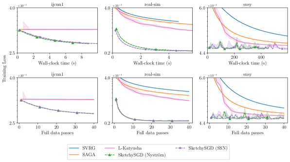
Figure 2: Comparisons to competitor methods with default learning rates (SVRG, SAGA) and smoothness parameters (L-Katyusha) on $l_{2}$-regularized logistic regression.

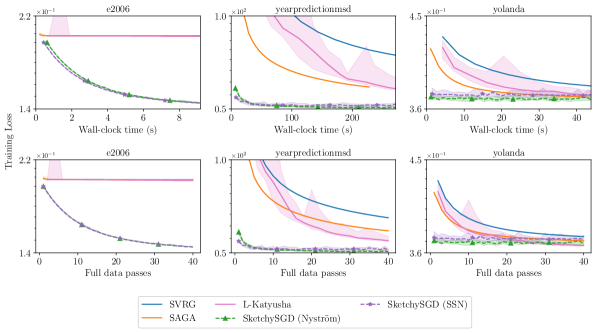
Figure 3: Comparisons to competitor methods with default learning rates (SVRG, SAGA) and smoothness parameters (L-Katyusha) on ridge regression.

5.2 SketchySGD matches or outperforms tuned competitor methods

In this section, we compare SketchySGD to SGD, SVRG, SAGA, L-Katyusha, and SLBFGS with their learning rate/smoothness hyperparameter tuned via grid search. For the tuned competitor methods, we only show the curve corresponding to the lowest attained training loss.

The results of these experiments are presented in Figs. 4 and 5. We observe that SketchySGD (Nyström) and SketchySGD (SSN) generally match or outperform the tuned competitor methods. SketchySGD (Nyström) and SketchySGD (SSN) outperform the competitor methods on E2006-tfidf and YearPredictionMSD, while performing comparably on both yolanda and susy. On ijcnn1, SketchySGD (Nyström) and SketchySGD (SSN) are outperformed temporarily by SLBFGS; however SLBFGS eventually diverges at its best learning rate for ijcnn1 and across the other datasets. On real-sim, we find that SGD and SAGA perform better than SketchySGD (Nyström) and SketchySGD (SSN) in terms of wall clock time, but perform similarly on gradient computations.

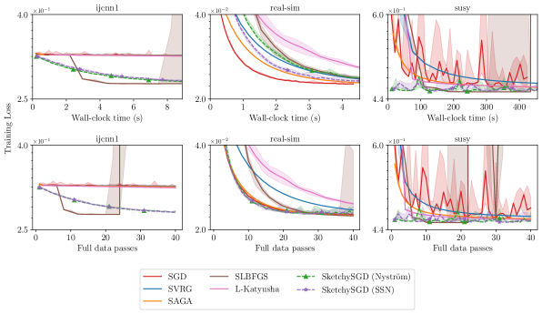
Figure 4: Comparisons to competitor methods with tuned learning rates (SGD, SVRG, SAGA, SLBFGS) and smoothness parameters (L-Katyusha) on $\ell^{2}$-regularized logistic regression.

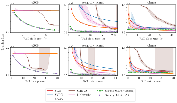
Figure 5: Comparisons to competitor methods with tuned learning rates (SGD, SVRG, SAGA, SLBFGS) and smoothness parameters (L-Katyusha) on ridge regression.

5.3 SketchySGD outperforms competitor methods on large-scale data

We apply random Fourier features to the HIGGS dataset, for which $(n_{\mathrm{tr}},p)=(1.05\cdot 10^{7},28)$, to obtain a transformed dataset with size $(n_{\mathrm{tr}},p)=(1.05\cdot 10^{7},10^{4})$. This transformed dataset is $840$ GB, larger than the hard drive and RAM capacity of most computers. To optimize, we load the original HIGGS dataset in memory and at each iteration, form a minibatch of the transformed dataset by applying the random features transformation to a minibatch of HIGGS. In this setting, computing a full gradient of the objective is computationally prohibitive. We exclude SVRG, L-Katyusha, and SLBFGS since they require full gradients.

We compare SketchySGD to SGD and SAGA with both default learning rates (SAGA only) and tuned learning rates (SGD and SAGA) via grid search. In this case, we only use $1$ random seed due to the sheer size of the problem.

Figs. 6 and 7 show these two sets of comparisons. We only plot test loss, as computing the training loss suffers from the same computational issues as computing a full gradient. The plots with respect to wall-clock time only show the time taken in optimization; they do not include the time taken in repeatedly applying the random features transformation. We find that SGD and SAGA make little to no progress in decreasing the test loss, even after tuning. However, both SketchySGD (Nyström) and SketchySGD (SSN) are able to decrease the test loss significantly. Furthermore, SketchySGD (Nyström) is able to achieve a similar test loss to SketchySGD (SSN) while taking less time, confirming that SketchySGD (Nyström) can be more efficient than SketchySGD (SSN) in solving large problems.

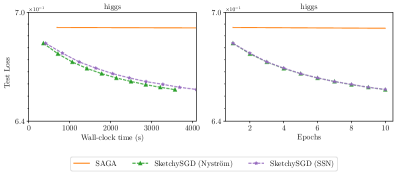
Figure 6: Comparison between SketchySGD and SAGA with default learning rate.

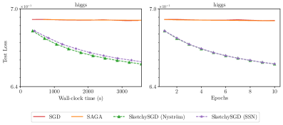
Figure 7: Comparison between SketchySGD, SGD and SAGA with tuned learning rates.

5.4 Sensitivity to rank and update frequency

In this section, we investigate the sensitivity of SketchySGD to the rank hyperparameter $r$ (Section 5.4.1) and update frequency hyperparameter $u$ (Section 5.4.2). In the first set of sensitivity experiments, we select ranks $r\in\{1,2,5,10,20,50\}$ while holding the update frequency fixed at $u=\left\lceil\frac{n_{\textrm{tr}}}{b_{g}}\right\rceil$ (1 epoch). In the second set of sensitivity experiments, we select update frequencies $u\in\left\{0.5\left\lceil\frac{n_{\textrm{tr}}}{b_{g}}\right\rceil,\left\lceil\frac{n_{\textrm{tr}}}{b_{g}}\right\rceil,2\left\lceil\frac{n_{\textrm{tr}}}{b_{g}}\right\rceil,5\left\lceil\frac{n_{\textrm{tr}}}{b_{g}}\right\rceil,\infty\right\}$, while holding the rank fixed at $r=10$. We use the same datasets as Sections 5.1 and 5.2. Each curve is the median performance of a given $(r,u)$ pair across $10$ random seeds (except for susy, which uses $3$ seeds), run for $40$ epochs.

5.4.1 Effects of changing the rank

Looking at Fig. 8, we see two distinct patterns: either increasing the rank has no noticeable impact on performance (E2006-tfidf, real-sim), or increasing the rank leads to faster convergence to a ball of noise around the optimum (YearPredictionMSD). We empirically observe that these patterns are related to the spectrum of each dataset, as shown in Fig. 9. For example, the spectrum of E2006-tfidf is highly concentrated in the first singular value, and decays rapidly, increased rank does not improve convergence. On the other hand, the spectrum of YearPredictionMSD is not as concentrated in the first singular value, but still decays rapidly, so convergence improves as we increase the rank from $r=1$ to $r=10$, after which performance no longer improves, in fact it slightly degrades. The spectrum of real-sim decays quite slowly in comparison to E2006-tfidf or YearPredictionMSD, so increasing the rank up to $50$ does not capture enough of the spectrum to improve convergence. One downside in increasing the rank is that the quantity $\eta_{\textrm{SketchySGD}}$ (3) can become large, leading to SketchySGD taking a larger step size. As a result, SketchySGD oscillates more about the optimum, as seen in YearPredictionMSD (Fig. 8). Last, Fig. 8 shows $r=10$ delivers great performance across all datasets, supporting its position as the recommended default rank. Rank sensitivity plots for yolanda, ijcnn1, and susy appear in Appendix F.

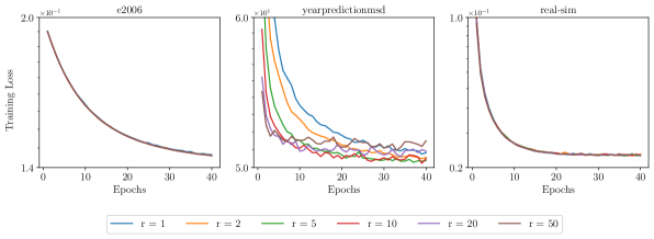
Figure 8: Sensitivity of SketchySGD to rank $r$.

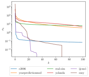
Figure 9: Top $100$ singular values of datasets after preprocessing.

5.4.2 Effects of changing the update frequency

In this section, we display results only for logistic regression (Figure 10), since there is no benefit to updating the preconditioner for a quadratic problem such as ridge regression (Appendix F): the Hessian in ridge regression is constant for all $w\in\mathbb{R}^{p}$. The impact of the update frequency depends on the spectrum of each dataset. The spectra of ijcnn1 and susy are highly concentrated in the top $r=10$ singular values and decay rapidly (Fig. 9), so even the initial preconditioner approximates the curvature of the loss well throughout optimization. On the other hand, the spectrum of real-sim decays quite slowly, and the initial preconditioner does not capture most of the curvature information in the Hessian. Hence for real-sim it is beneficial to update the preconditioner, however only infrequent updating is required, as an update frequency of 5 epochs yields almost identical performance to updating every half epoch. So, increasing the update frequency of the preconditioner past a certain threshold does not improve performance, it just increases the computational cost of the algorithm. Last, $u=\lceil\frac{n_{\textrm{ntr}}}{b_{g}}\rceil$ exhibits consistent excellent performance across all datasets, supporting the recommendation that it be the default update frequency.

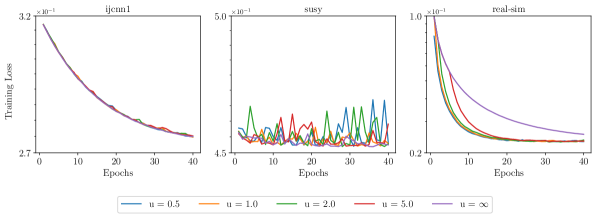
Figure 10: Sensitivity of SketchySGD to update frequency $u$.

6 Conclusion

In this paper, we have presented SketchySGD, a fast and robust stochastic quasi-Newton method for convex machine learning problems. SketchySGD uses subsampling and randomized low-rank approximation to improve conditioning by approximating the curvature of the loss. Furthermore, SketchySGD uses a novel automated learning rate and comes with default hyperparameters that enable it to work out of the box without tuning.

SketchySGD has strong benefits both in theory and in practice. In the least-squares setting, our theory shows that SketchySGD converges to a neighborhood of the optimum at a faster rate than SGD, and our experiments validate this improved convergence rate. SketchySGD with its default hyperparameters outperforms or matches the performance of SGD, SAGA, SVRG, SLBFGS, and L-Katyusha (the last four of which use variance reduction), even when optimizing the learning rate for the competing methods using grid search.

Appendix A RandNysApprox

In this section we provide the pseudocode for the RandNysApprox algorithm mentioned in Section 2, which SketchySGD uses to construct the low-rank approximation $\hat{H}_{S_{k}}$.

Algorithm 3 RandNysApprox

  Input: sketch $Y$ of $H_{S_{k}}$, orthogonalized test matrix $Q$, rank $r_{k}$

  $\nu=\sqrt{p}\text{eps}(\text{norm}(Y,2))$ {Compute shift}

  $Y_{\nu}=Y+\nu Q$ {Add shift for stability}

  $C=\text{chol}(Q^{T}Y_{\nu})$ {Cholesky decomposition}

  $B=Y/C$ {Triangular solve}

  $[\hat{V},\Sigma,\sim]=\text{svd}(B,0)$ {Thin SVD}

  $\hat{\Lambda}=\text{max}\{0,\Sigma^{2}-\nu I\}$ {Remove shift, compute eigs}

  Return: $\hat{V},\hat{\Lambda}$

Algorithm 3 follows [50]. $\text{eps}(x)$ is defined as the positive distance between $x$ and the next largest floating point number of the same precision as $x$. The test matrix $Q$ is the same test matrix used to generate the sketch $Y$ of $H_{S_{k}}$. The resulting Nyström approximation $\hat{H}_{S_{k}}$ is given by $\hat{V}\hat{\Lambda}\hat{V}^{T}$. The resulting Nyström approximation is psd but may have eigenvalues that are equal to $0$. In our algorithms, this approximation is always used in conjunction with a regularizer to ensure positive definiteness.

Appendix B Proofs not appearing in the main paper

In this section, we give the proofs of claims that are not present in the main paper.

B.1 Proof that SketchySGD is SGD in preconditioned space

Here we give the proof of (2) from Section 1. As in the prequel, we set $P_{k}=\hat{H}^{\rho}_{S_{k}}$ in order to avoid notational clutter. Recall the SketchySGD update is given by

$$w_{k+1}=w_{k}-\eta_{j}P_{j}^{-1}g_{B_{k}},$$

where $\mathbb{E}_{B_{k}}[g_{B_{k}}]=g_{k}$. We start by making the following observation about the SketchySGD update.

Lemma B.1 (SketchySGD is SGD in preconditioned space).

At outer iteration $j$ define $f_{P_{j}}(z)=f(P_{j}^{-1/2}z)$, that is define the change of variable $w=P_{j}^{-1/2}z$. Then,

$$g_{P_{j}}(z)=P_{j}^{-1/2}g(P_{j}^{-1/2}z)=P^{-1/2}_{j}g(w)$$

$$H_{P_{j}}(z)=P_{j}^{-1/2}H(P_{j}^{-1/2}z)P_{j}^{-1/2}=P_{j}^{-1/2}H(w)P^{-1/2}_{j}.$$

Hence the SketchySGD update may be realized as

$$z_{k+1}=z_{k}-\eta_{j}\hat{g}_{P_{j}}(z_{k})$$

$$w_{k+1}=P_{j}^{-1/2}z_{k+1},$$

where $\hat{g}_{P_{j}}(z_{k})=P_{j}^{-1/2}g_{B_{k}}(P_{j}^{-1/2}z_{k}).$

Proof B.2.

The first display of equations follow from the definition of the change of variable and the chain rule, while the last display follows from definition of the SketchySGD update and the first display.

B.2 Proof of Lemma 4.4

Below we provide the proof of Lemma 4.4.

Proof B.3.

We start by observing the following relation in the Loewner ordering,

$$\nabla^{2}f_{i}(w)\preceq nH(w)\quad\forall i\in\{1,\dots,n\}.$$

The preceding display immediately implies

$$\nabla^{2}f_{i}(w)+\rho I\preceq n\left(H(w)+\rho I\right).$$

Conjugating both sides by $(H^{\rho})^{-1/2}$, we reach

$$\left(H(w)+\rho I\right)^{-1/2}\left(\nabla^{2}f_{i}(w)+\rho I\right)\left(H(w)+\rho I\right)^{-1/2}\preceq nI.$$

It now immediately follows that $\tau_{\rho}(H(w))\leq n$. On the other hand, for all $i\in\{1,\dots n\}$ we have

$$\nabla^{2}f_{i}(w)+\rho I\preceq\left(\lambda_{1}\left(\nabla^{2}f_{i}(w)\right)+\rho\right)I\preceq\left(M(w)+\rho\right)I,$$

where the last relation follows by definition of $M(w)$. So, conjugating by $\left(H^{\rho}(w)\right)^{-1/2}$ we reach

$$\left(H^{\rho}(w)\right)^{-1/2}\left(\nabla^{2}f_{i}(w)+\rho I\right)\left(H^{\rho}(w)\right)^{-1/2}\preceq\left(M(w)+\rho\right)\left(H(w)+\rho I\right)^{-1}\preceq\frac{M(w)+\rho}{\mu+\rho}I,$$

which immediately yields $\tau_{\rho}(H(w))\leq\frac{M(w)+\rho}{\mu+\rho}$. Thus combining both bounds, we conclude

$$\tau_{\rho}\left(H(w)\right)\leq\min\left\{n,\frac{M(w)+\rho}{\mu+\rho}\right\}.$$

B.3 Proof of Proposition 4.5

We first recall the definition of a sub-Gaussian random matrix [52].

Definition B.4 (Sub-Gaussian random matrix).

A non-zero symmetric matrix $A\in\mathbb{R}^{p\times p}$ is said to be sub-Gaussian with matrix-parameter $\mathcal{V}\in\mathbb{S}^{++}_{p}(\mathbb{R})$, if

$${\mathbb{E}}[\textup{e}^{t(A-{\mathbb{E}}[A])}]\preceq\textup{e}^{\frac{t^{2}\mathcal{V}}{2}},\quad\forall t\in\mathbb{R}.$$

Sub-Gaussian random matrices are known to satisfy the following tail-bound, which is a matrix analogue of Hoeffding’s inequality. It is a special case of [52, Theorem 6.15, p. 174].

Theorem B.5 (Matrix Hoeffding inequality, Theorem 6.15 (Wainwright, 2019) [52]).

Let $\{A_{i}\}^{N}_{i=1}$ be a sequence of $p\times p$ i.i.d. mean-zero $\mathcal{V}$-sub-Gaussian random matrices. Then for all $t>0$

$${\mathbb{P}}\left(\left\|\frac{1}{N}\sum_{i=1}^{N}\left(A_{i}-{\mathbb{E}}[A]\right)\right\|\geq t\right)\leq 2p\textrm{e}^{\frac{-Nt^{2}}{2\nu^{2}}},$$

where $\nu=\|\mathcal{V}\|$.

Proof B.6.

By hypothesis $\nabla^{2}\ell(z;w)$ is $\nu^{2}$-sub-Gaussian, and the $z_{i}$’s are i.i.d.. Hence we may invoke Theorem B.5 with $N=1$ and $t=\rho\sqrt{2\nu^{2}n\log\left(\frac{2np}{\delta}\right)}$ to reach

$$\|\nabla^{2}f_{i}(w)-{\mathbb{E}}[\nabla^{2}\ell(z;w)]\|\leq\rho\sqrt{2\nu^{2}n\log\left(\frac{2np}{\delta}\right)},$$

with probability at least $1-2p\exp{\left(-n\rho^{2}\log\left(\frac{2np}{\delta}\right)\right)}\geq 1-\frac{\delta}{n}$, where the last inequality uses $\rho\geq\frac{1}{\sqrt{n}}$. So, by union bound

$$\|\nabla^{2}f_{i}(w)-{\mathbb{E}}[\nabla^{2}\ell(z;w)]\|\leq\rho\sqrt{2\nu^{2}n\log\left(\frac{2np}{\delta}\right)}\quad\forall i\in\{1,\dots,n\},$$

with probability at least $1-\delta$. Consequently

$$\|\nabla^{2}f_{i}(w)-\nabla^{2}f_{j}(w)\|\leq\rho\sqrt{8\nu^{2}n\log\left(\frac{2np}{\delta}\right)},\quad\forall i\neq j.$$

with probability at least $1-\delta$. This in turn implies

$$\|\nabla^{2}f_{i}(w)-H(w)\|\leq\rho\sqrt{8\nu^{2}n\log\left(\frac{2np}{\delta}\right)}\quad\forall i\in\{1,\dots,n\},$$

with the same failure probability. Now, let us condition on the good event

$$\mathcal{G}=\left\{\|\nabla^{2}f_{i}(w)-H(w)\|\leq\rho\sqrt{8\nu^{2}n\log\left(\frac{2np}{\delta}\right)},\quad\forall i\in\{1,\dots,n\}\right\}.$$

Further let us set $E_{i}=\nabla^{2}f_{i}(w)-H(w)$. Then for any $i\in\{1,\dots,n\}$, we have

$$\lambda_{1}\left((H(w)+\rho I)^{-1/2}(\nabla^{2}f_{i}(w)+\rho I)(H(w)+\rho I)^{-1/2}\right)=$$

$$=\lambda_{1}\left((H(w)+\rho I)^{-1/2}(H(w)+E_{i}+\rho I)(H(w)+\rho I)^{-1/2}\right)\overset{(1)}{\leq}$$

$$1+\lambda_{1}\left((H(w)+\rho I)^{-1/2}E_{i}(H(w)+\rho I)^{-1/2}\right)\overset{(2)}{\leq}$$

$$1+\left\|(H(w)+\rho I)^{-1/2}E_{i}(H(w)+\rho I)^{-1/2}\right\|\overset{(3)}{\leq}1+\|P^{-1}\|\|E_{i}\|$$

$$\overset{(4)}{\leq}1+\frac{\rho\sqrt{8\nu^{2}n\log\left(\frac{2np}{\delta}\right)}}{\rho}=1+\sqrt{8\nu^{2}n\log\left(\frac{2np}{\delta}\right)}.$$

Here $(1)$ uses Weyl’s inequalities, $(2)$ uses $\lambda_{1}(M)\leq\|M\|$ for any symmetric matrix $M$, $(3)$ uses Cauchy-Schwarz, and $(4)$ uses that we are conditioned on $\mathcal{G}$ and $\|P^{-1}\|\leq\rho^{-1}$. Hence $\tau_{\rho}(H(w))\leq 1+\sqrt{8\nu^{2}n\log\left(\frac{2np}{\delta}\right)}$. The desired claim now immediately follows, as $\mathcal{G}$ holds with probability at least $1-\delta$.

B.4 Proof of Lemma 4.6

The proof is based on a standard matrix concentration argument. To this end, we first recall the following matrix Chernoff inequalities due to Tropp [48, 49].

Proposition B.7 (Theorem 5.1.1, Tropp (2015) [49]).

Let $X_{1},\cdots,X_{m}$ be a sequence of independent, symmetric $p\times p$ random matrices satisfying $0\preceq X_{i}\preceq KI$. Set $Y=\sum^{m}_{i=1}X_{i}$, $\gamma_{\textup{min}}=\lambda_{p}({\mathbb{E}}[Y])$, and $\gamma_{\textup{max}}=\lambda_{1}({\mathbb{E}}[Y])$. Then

$$\mathbb{P}\left(\lambda_{p}(Y)\leq(1-\zeta)\gamma_{\textup{min}}\right)\leq p\exp\left(\frac{-\zeta^{2}\gamma_{\textup{min}}}{2K}\right),$$

and

$$\mathbb{P}\left(\lambda_{1}(Y)\geq(1+\zeta)\gamma_{\textup{max}}\right)\leq p\exp\left(\frac{-\zeta^{2}\gamma_{\textup{max}}}{3K}\right).$$

Proof of Lemma 4.6

With the matrix Chernoff inequalities in hand, we now commence the proof.

Proof B.8.

By construction, the regularized subsampled Hessian is given by

$$H_{S}^{\rho}(w)=\frac{1}{b_{h}}\sum_{i\in S}\nabla^{2}f_{i}(w)+\rho I.$$

Define $X_{i}=\frac{1}{b_{h}}(H^{\rho})^{-1/2}\left(\nabla^{2}f_{i}(w)+\rho I)\right)(H^{\rho})^{-1/2}$. Then,

$$(H^{\rho})^{-1/2}H^{\rho}_{S}(H^{\rho})^{-1/2}=\sum_{i}X_{i}\coloneqq Y.$$

Observe that ${\mathbb{E}}[Y]=I$ and $0\preceq X_{i}\preceq\frac{\tau_{\rho}(H(w))}{b_{h}}$, where the latter inequality follows by definition of $\tau_{\rho}(H(w))$. Hence, by the matrix Chernoff bound

$$\mathbb{P}\left(\lambda_{p}(Y)\leq(1-\zeta)\right)\leq p\exp\left(\frac{-b_{h}\zeta^{2}}{2\tau_{\rho}(H(w))}\right).$$

Setting $b_{h}=\frac{2\tau_{\rho}(H(w))\left(\log\left(\frac{2p}{\delta}\right)\right)}{\zeta^{2}}$, we find

$$\lambda_{p}(Y)\geq 1-\zeta\quad\text{with probability at least}\hskip 3.0pt1-\delta/2.$$

Similarly, setting $b_{h}=\frac{3\tau_{\rho}(H(w))\left(\log\left(\frac{2p}{\delta}\right)\right)}{\zeta^{2}}$, we find

$$\lambda_{1}(Y)\leq 1+\zeta\quad\text{with probability at least}\hskip 3.0pt1-\delta/2.$$

Thus, with batch size $b_{h}=\frac{3\tau_{\rho}(H(w))\left(\log\left(\frac{2p}{\delta}\right)\right)}{\zeta^{2}}$, we conclude

$$(1-\zeta)I\preceq Y\preceq(1+\zeta)I$$

with probability at least $1-\delta$. Conjugating, we find

$$(1-\zeta)H^{\rho}\preceq H^{\rho}_{S}\preceq(1+\zeta)H^{\rho},$$

which is equivalent to

$$\frac{1}{1+\zeta}H_{S}^{\rho}\preceq H^{\rho}\preceq\frac{1}{1-\zeta}H^{\rho}_{S}.$$

Now as $\zeta\in(0,1)$ is arbitrary, the preceding bound also holds when we replace $\zeta$ by $\zeta^{\prime}=\frac{\zeta}{1+\zeta}$. Note that $\zeta^{\prime}$ satisfies

$$1-\zeta\leq\frac{1}{1+\zeta^{\prime}}\leq\frac{1}{1-\zeta^{\prime}}\leq 1+\zeta.$$

So, by scaling $\zeta$ by $\frac{1}{1+\zeta}$ we obtain

$$\left(1-\zeta\right)H_{S}^{\rho}\preceq H^{\rho}\preceq\left(1+\zeta\right)H^{\rho}_{S}.$$

Now as $\zeta\in(0,1)$, it holds that $O\left(\frac{(1+\zeta)^{2}}{\zeta^{2}}\right)=O\left(\frac{1}{\zeta^{2}}\right)$. Hence when $b_{h}=O\left(\frac{\tau_{\rho}(H(w))\log\left(\frac{p}{\delta}\right)}{\zeta^{2}}\right)$

$$\left(1-\zeta\right)H_{S}^{\rho}\preceq H^{\rho}\preceq\left(1+\zeta\right)H^{\rho}_{S},$$

holds with probability at least $1-\delta$.

B.5 Proof of Proposition 4.7 and Corollary 4.8

The proof of Proposition 4.7 has two layers. First we show that $\hat{H}_{S_{k}}^{\rho}$ is close to $H^{\rho}_{S_{k}}$, then we argue that $\hat{H}^{\rho}_{S_{k}}$ is close to $H^{\rho}_{k}$, as $H^{\rho}_{S_{k}}$ is close $H_{k}^{\rho}$, thanks to Lemma 4.6. Proposition 4.7 is then established by relating $H_{k}^{\rho}$ to $H_{k}$, further Corollary 4.8 immediately follows via a union bound argument.

In order to relate $\hat{H}^{\rho}_{S_{k}}$ to $H_{S_{k}}$, we need to control the error resulting from the low-rank approximation. To accomplish this, we recall the following result from [56].

Lemma B.9 (Controlling low-rank approximation error, Lemma A.7 Zhao et al. (2022) [56]).

Let $\tau>0$ and $E_{k}=H_{S_{k}}-\hat{H}_{S_{k}}$. Construct a randomized Nyström approximation from a standard Gaussian random matrix $\Omega$ with rank $r_{k}=O(d_{\textup{eff}}(\tau)+\log(\frac{1}{\delta}))$. Then the event

(10) $$\mathcal{E}^{(2)}_{k}=\{\|E_{k}\|\leq\tau\}$$

holds with probability at least $1-\delta$.

Lemma B.9 allows us to establish the following result, which shows our low-rank approximation is close to the regularized subsampled Hessian in the Loewner ordering.

Lemma B.10 (Closeness in Loewner ordering between $H_{S_{k}}$ and $\hat{H}_{S_{k}}^{\rho}$).

Let $0<\zeta<1$. Suppose at iteration $k$ SketchySGD uses a low-rank approximation $\hat{H}_{S_{k}}$ to $H_{S_{k}}$ with rank $r_{k}=O(d_{\textup{eff}}(\zeta\rho)+\log(\frac{1}{\delta}))$. Then with probability at least $1-\delta$,

(11) $$(1-\zeta)\hat{H}_{S_{k}}^{\rho}\preceq H^{\rho}_{S_{k}}\preceq(1+\zeta)\hat{H}_{S_{k}}^{\rho}$$

Proof B.11.

Let $E_{k}=H_{S_{k}}-\hat{H}_{S_{k}}$, and note by the properties of the Nyström approximation that $E_{k}\succeq 0$ [50, 15]. Now, notice the event

$$\mathcal{E}^{(2)}_{k}=\{\|E_{k}\|\leq\zeta\rho\}$$

holds with probability at least $1-\delta$ by Lemma B.9. Henceforth, all analysis is conditioned on $\mathcal{E}^{(2)}_{k}$, and therefore the conclusions hold with probability at least $1-\delta$. Now, the regularized Hessian and approximate Hessian satisfy

(12) $$H_{S_{k}}^{\rho}=\hat{H}^{\rho}_{S_{k}}+E_{k},$$

Let $P=\hat{H}^{\rho}_{S_{k}}$. Then combining (12) with Weyl’s inequalities yields

$$\lambda_{1}(P^{-1/2}H_{S_{k}}^{\rho}P^{-1/2})\leq\lambda_{1}\left(P^{-1/2}\hat{H}^{\rho}_{S_{k}}P^{-1/2}\right)+\lambda_{1}\left(P^{-1/2}E_{k}P^{-1/2}\right)=$$

$$1+\|P^{-1/2}E_{k}P^{-1/2}\|\leq 1+\|P^{-1}\|\|E_{k}\|\leq 1+\frac{\|E_{k}\|}{\rho}\leq 1+\zeta.$$

To bound the smallest eigenvalue, observe that

$$H_{S_{k}}^{\rho}\succeq\hat{H}^{\rho}_{S_{k}}\quad\implies\quad H_{S_{k}}^{\rho}\succeq P.$$

Thus, conjugating the preceding relation by $P^{-1/2}$ we obtain

$$P^{-1/2}H_{S_{k}}^{\rho}P^{-1/2}\succeq I_{p},$$

where $I_{p}$ is the $p\times p$ identity matrix. The preceding inequality immediately yields

$$\lambda_{p}(P^{-1/2}H_{S_{k}}^{\rho}P^{-1/2})\geq 1.$$

Hence,

$$1\leq\lambda_{p}(P^{-1/2}H_{S_{k}}^{\rho}P^{-1/2})\leq\lambda_{1}(P^{-1/2}H_{S_{k}}^{\rho}P^{-1/2})\leq 1+\zeta.$$

As an immediate consequence, we obtain the Loewner ordering relation

$$I_{p}\preceq P^{-1/2}H_{S_{k}}^{\rho}P^{-1/2}\preceq(1+\zeta)I_{p}$$

which we conjugate by $P^{1/2}$ to show

$$\hat{H}^{\rho}_{S_{k}}\preceq H_{S_{k}}^{\rho}\preceq(1+\zeta)\hat{H}^{\rho}_{S_{k}}.$$

The claimed result follows.

Proof of Proposition 4.7

With Lemmas 4.6 and B.9 in hand, we now commence the proof of Proposition 4.7.

Proof B.12.

Combining Lemma 4.6 and Lemma B.10, we find

$$(1-\zeta)^{2}\hat{H}^{\rho}_{S_{k}}\preceq H_{k}^{\rho}\preceq(1+\zeta)^{2}\hat{H}_{S_{k}}^{\rho},$$

with probability at least $1-2\delta$. Now, observing that

$$H_{k}^{\rho}\preceq\left(1+\frac{\rho}{\mu}\right)H_{k},$$

we conclude

$$(1-\zeta)^{2}\frac{\mu}{\mu+\rho}\hat{H}_{S_{k}}^{\rho}\preceq H_{k}\preceq(1+\zeta)^{2}\hat{H}_{S_{k}}^{\rho}.$$

The desired claim follows by scaling $\delta$ and $\zeta$ appropriately.

Proof B.13.

Instating the hypotheses of Lemma 4.6 and Lemma B.10 with $\delta^{\prime}=\frac{\delta}{2T}$, we obtain for each $k\in\{0,\ldots,T-1\}$ that

$${\mathbb{P}}(\mathcal{E}_{k}^{C})\leq\frac{\delta}{T}.$$

Consequently,

$${\mathbb{P}}(\mathcal{E}_{T})=1-{\mathbb{P}}(\mathcal{E}_{T}^{C})\geq 1-\sum^{T-1}_{k=0}\frac{\delta}{T}=1-\delta.$$

B.6 Proof of Lemma 4.11

Proof B.14.

By relative convexity of $f$, we have that

$$f(w_{\star})\geq f(w_{k})+\langle\nabla f(w_{k}),w_{\star}-w_{k}\rangle+\frac{\hat{\mu}}{2}\|w_{\star}-w_{k}\|_{H(w_{k})}^{2}.$$

Hence we have

$$f(w_{\star})\geq f(w_{k})+\langle P_{k}^{-1}\nabla f(w_{k}),w_{\star}-w_{k}\rangle_{P_{k}}+\frac{\hat{\mu}}{2}\|P_{k}^{1/2}\left(w_{\star}-w_{k}\right)\|_{P_{k}^{-1/2}H(w_{k})P^{-1/2}_{k}}^{2}\geq$$

$$f(w_{k})+\langle P_{k}^{-1}\nabla f(w_{k}),w_{\star}-w_{k}\rangle_{P_{k}}+\frac{\hat{\mu}}{2}\frac{(1-\zeta)\mu}{\mu+\rho}\|w_{\star}-w_{k}\|_{P_{k}}^{2},$$

where in the last inequality we have used that the conclusion of Proposition 4.7 holds. The claim now follows by recalling that $\hat{\mu}_{P}=\frac{(1-\zeta)\mu}{\mu+\rho}\hat{\mu}$.

B.7 Proof of Lemma 4.9

Proof B.15.

Observe each $f_{i}$ is $L_{i}$-smooth, and $P_{k}\succeq\rho I$ for all $k\geq 0$. So by the conjugation rule, for each $i\in\{1,\cdots n\}$ and any $k\geq 0$

$$\lambda_{1}\left(P_{k}^{-1/2}\nabla^{2}f_{i}(w)P^{-1/2}_{k}\right)\leq\frac{L_{i}}{\rho}.$$

Hence

$$X_{P_{k_{i}}}\leq\frac{L_{i}}{\rho}\quad\text{with probability 1}.$$

Thus, $L_{P_{i}}<\infty.$

The claim for $L_{P_{\textup{max}}}$ follows analogously by observing

$$X_{P_{k_{i}}}\leq\frac{L_{\textrm{max}}}{\rho}\quad\text{with probability 1},$$

for all $i\in\{1,\cdots,n\}$.

B.8 Proof of Proposition 4.10

In this subsection we prove Proposition 4.10, which controls the variance of the preconditioned minibatch gradient. An essential ingredient to the proof is the following result due to [18], which controls the minibatch gradient variance in the usual Euclidean norm.

Proposition B.16 (Controlling minibatch gradient variance, Proposition 3.8 [18]).

Suppose each $f_{i}$ is convex and satisfies

$$f_{i}(w+h)\leq f_{i}(w)+\langle\nabla f_{i}(w),h\rangle+\frac{1}{2}\|h\|_{M_{i}}^{2},\quad\forall w,h\in\mathbb{R}^{p},$$

for some symmetric positive definite matrix $M_{i}$. Further, suppose we construct the gradient sample $g_{B_{k}}$ with batch-size $b_{g}$. Then for every $w\in\mathbb{R}^{p}$,

$$\mathbb{E}_{B_{k}}\|g_{B_{k}}(w)-g_{B_{k}}(w_{\star})\|^{2}\leq 2\mathcal{L}(f(w)-f(w_{\star})),$$

$$\mathbb{E}_{B_{k}}\|g_{B_{k}}(w)\|^{2}\leq 4\mathcal{L}(f(w)-f(w_{\star}))+2\sigma^{2}$$

where

$$\mathcal{L}\leq\frac{n(b_{g}-1)}{b_{g}(n-1)}\lambda_{1}\left(\frac{1}{n}\sum_{i=1}^{n}M_{i}\right)+\frac{n-b_{g}}{b_{g}(n-1)}\textup{max}_{1\leq i\leq n}\lambda_{1}(M_{i})$$

and

$$\sigma^{2}=\frac{1}{b_{g}}\frac{n-b_{g}}{n-1}\frac{1}{n}\sum_{i=1}^{n}\|\nabla f_{i}(w_{\star})\|^{2}.$$

Proof B.17.

Define $f_{P_{k_{i}}}(z)=f_{i}(P_{k}^{-1/2}z)$. By hypothesis we have in preconditioned space that each $f_{P_{k_{i}}}(z)$ satisfies:

$$f_{P_{k_{i}}}(z+h)\leq f_{P_{k_{i}}}(z)+\langle\nabla f_{P_{k_{i}}}(z),h\rangle+\frac{1}{2}\|h\|^{2}_{M_{i}}\quad\forall z,h\in\mathbb{R}^{n},$$

where $M_{i}=L_{P_{k_{i}}}I$. This follows as in preconditioned space each $f_{P_{k_{i}}}(z)$ is $L_{P_{k_{i}}}$-smooth with

$$L_{P_{k_{i}}}=\sup_{w\in\mathbb{R}^{p}}\lambda_{1}\left(P_{k}^{-1/2}\nabla^{2}f_{i}(w)P_{k}^{-1/2}\right).$$

Now, applying Proposition B.16 in preconditioned space, we find

$$\mathbb{E}_{k}\|\hat{g}_{P_{k}}(z_{k})-\hat{g}_{P_{k}}(z_{\star})\|^{2}\leq 2\mathcal{L}_{P_{k}}\left(f_{P_{k}}(z_{k})-f_{P_{k}}(z_{\star})\right),$$

$$\mathbb{E}_{k}\|\hat{g}_{P_{k}}(z_{k})\|^{2}\leq 4\mathcal{L}_{P_{k}}\left(f_{P_{k}}(z_{k})-f_{P_{k}}(z_{\star})\right)+2\sigma_{P_{k}}^{2}.$$

Here

$$\mathcal{L}_{P_{k}}\leq\frac{n(b_{g}-1)}{b_{g}(n-1)}\frac{1}{n}\sum_{i=1}^{n}L_{P_{k_{i}}}+\frac{n-b_{g}}{b_{g}(n-1)}\textup{max}_{1\leq i\leq n}\lambda_{1}\left(P_{k}^{-1/2}\nabla^{2}f_{i}(w_{k})P_{k}^{-1/2}\right),$$

and

$$\sigma_{P_{k}}^{2}=\frac{1}{b_{g}}\frac{n-b_{g}}{n-1}\frac{1}{n}\sum_{i=1}^{n}\|\nabla f_{i}(z_{\star})\|^{2}.$$

Recalling from Lemma B.1 that $\hat{g}_{P_{k}}(z)=P_{k}^{-1/2}g_{B_{k}}(w)$, $f_{P_{k}}(z_{k})-f_{P_{k}}(z_{\star})=f(w_{k})-f(w_{\star})$, and using $P^{1/2}_{k}\succeq\sqrt{\rho}I$, the variance bounds in preconditioned space become:

$$\mathbb{E}_{k}\|g_{B_{k}}(w_{k})-g_{B_{k}}(w_{\star})\|_{P_{k}^{-1}}^{2}\leq 2\mathcal{L}_{P_{k}}\left(f(w_{k})-f(w_{\star})\right),$$

$$\mathbb{E}_{k}\|\hat{g}_{B_{k}}(w_{k})\|^{2}_{P_{k}^{-1}}\leq 4\mathcal{L}_{P_{k}}\left(f(w_{k})-f(w_{\star})\right)+\frac{2\sigma^{2}}{\rho},$$

where $\sigma^{2}$ is as in Proposition B.16. Now, let $X_{\mathcal{L}_{P_{k}}}=\sup_{k\geq 0}\mathcal{L}_{P_{k}}$ and define $\mathcal{L}_{P}$ to be the smallest constant $C$ such that

$$X_{\mathcal{L}_{P_{k}}}\leq C\quad\text{with probability 1}.$$

Observe $\mathcal{L}_{P}$ is well-defined, as by Lemma 4.9

$$\mathcal{L}_{P_{k}}\leq\frac{n(b_{g}-1)}{b_{g}(n-1)}\frac{1}{n}\sum_{i=1}^{n}L_{P_{i}}+\frac{n-b_{g}}{b_{g}(n-1)}L_{P_{\textrm{max}}}$$

for all $k$ with probability 1. So with probability 1

$$X_{\mathcal{L}_{P_{k}}}\leq\mathcal{L}_{P}\leq\frac{n(b_{g}-1)}{b_{g}(n-1)}L_{P}+\frac{n-b_{g}}{b_{g}(n-1)}L_{P_{\textrm{max}}},$$

which concludes the proof.

Appendix C Experimental details

Here we provide more details regarding the experiments in Section 5.

Ridge regression datasets

The ridge regression experiments are run on the datasets described in the main text. E2006-tfidf and YearMSD’s rows are normalized to have unit-norm, while we standardize the features of yolanda. For YearPredictionMSD we use a ReLU random features transformation that gives us $4367$ features in total. For yolanda we use a random features transformation with bandwidth $1$ that gives us $1000$ features in total, and perform a random 80-20 split to form a training and test set. In Table 2, we provide the dimensions of the datasets, where $n_{\textrm{tr}}$ is the number of training samples, $n_{\textrm{test}}$ is the number of testing samples, and $d$ is the number of features.

Table 2: Dimensions of Ridge Regression Datasets

Dataset	$n_{\textrm{tr}}$	$n_{\textrm{test}}$	$d$
E2006-tfidf	$16087$	$3308$	$150360$
YearPredictionMSD	$463715$	$51630$	$4367$
yolanda	$320000$	$80000$	$1000$

Logistic regression datasets

The logistic regression experiments are run on the datasets described in the main text. All datasets’ rows are normalized so that they have unit norm. For ijcnn1 and susy we use a random features transformation with bandwidth $1$ that gives us $2500$ and $1000$ features, respectively. For real-sim, we use a random 80-20 split to form a training and test set. For HIGGS, we repeatedly apply a random features transformation with bandwidth $1$ to obtain $10000$ features, as described in Section 5.3. In Table 3, we provide the dimensions of the datasets, where $n_{\textrm{tr}}$ is the number of training samples, $n_{\textrm{test}}$ is the number of testing samples, and $d$ is the number of features.

Table 3: Dimensions of Logistic Regression Datasets

Dataset	$n_{\textrm{tr}}$	$n_{\textrm{test}}$	$d$
ijcnn1	$49990$	$91701$	$2500$
susy	$4500000$	$500000$	$1000$
real-sim	$57847$	$14462$	$20958$
HIGGS	$10500000$	$500000$	$10000$

Additional hyperparameters

For SVRG and SLFBGS we perform a full gradient computation at every epoch. For SLFBGS we update the inverse Hessian approximation every epoch and set the Hessian batch size to $\sqrt{n_{\mathrm{tr}}}$, which matches the Hessian batch size hyperparameter in SketchySGD. In addition, we follow [35] and set the memory size of SLFBGS to $10$. For L-Katyusha, we initialize the update probability $p=b_{g}/n_{\mathrm{tr}}$ to ensure the average number of iterations between full gradient computations is equal to one epoch. We follow [25] and set $\mu$ equal to the $\ell^{2}$-regularization parameter, $\sigma=\frac{\mu}{L},\theta_{1}=\min\{\sqrt{2\sigma n_{\mathrm{tr}}/3},\frac{1}{2}\}$, and $\theta_{2}=\frac{1}{2}$. All algorithms use a batch size of $256$ for computing stochastic gradients, except on the HIGGS dataset. For the HIGGS dataset, SGD, SAGA, and SketchySGD are all run with a batch size of $4096$.

Default hyperparameters for SAGA/SVRG/L-Katyusha

The theoretical analysis of SVRG, SAGA, and L-Katyusha all yield recommended learning rates that lead to linear convergence. In practical implementations such as scikit-learn [40], these recommendations are often taken as the default learning rate. For SAGA, we follow the scikit-learn implementation, which uses the following learning rate:

$$\eta=\max\left\{\frac{1}{3L},\frac{1}{2\left(L+n_{\textrm{tr}}\mu\right)}\right\},$$

where $L$ is the smoothness constant of $f$ and $\mu$ is the strong convexity constant. The theoretical analysis of SVRG suggests a step-size of $\eta=\frac{1}{10\mathcal{L}}$, where $\mathcal{L}$ is the expected-smoothness constant. We have found this setting to pessimistic relative to the SAGA default, so we use the same default for SVRG as we do for SAGA. For L-Katyusha the hyperparameters $\theta_{1}$ and $\theta_{2}$ are controlled by how we specify $L^{-1}$, the reciprocal of the smoothness constant. Thus, the default hyperparameters for all methods are controlled by how $L$ is specified.

Now, standard computations show that the smoothness constants for least-squares and logistic regression satisfy

$$L_{\textrm{least-squares}}\leq\frac{1}{n_{\textrm{tr}}}\sum_{i=1}^{n_{\textrm{tr}}}\|a_{i}\|^{2},$$

$$L_{\textrm{logistic}}\leq\frac{1}{4n_{\textrm{tr}}}\sum_{i=1}^{n_{\textrm{tr}}}\|a_{i}\|^{2}.$$

The scikit-learn software package uses the preceding upper-bounds in place of $L$ to set $\eta$ in their implementation of SAGA. We adopt this convention for setting the hyperparameters of SAGA, SVRG and L-Katyusha. We display the defaults for the three methods in Table 4.

Table 4: Default hyperparameters for SVRG/SAGA/L-Katyusha

Method\Dataset	E2006-tfidf	YearPredictionMSD	yolanda	ijcnn1	real-sim	susy	HIGGS
SVRG/SAGA	$4.95\cdot 10^{-1}$	$1.01\cdot 10^{0}$	$4.96\cdot 10^{-1}$	$1.91\cdot 10^{0}$	$1.93\cdot 10^{0}$	$1.87\cdot 10^{0}$	$1.93\cdot 10^{0}$
L-Katyusha	$1.00\cdot 10^{0}$	$4.85\cdot 10^{-1}$	$9.98\cdot 10^{-1}$	$2.52\cdot 10^{-1}$	$2.50\cdot 10^{-1}$	$2.57\cdot 10^{-1}$	N/A

Grid search parameters (Sections 5.1 and 5.2)

We choose the grid search ranges for SVRG, SAGA, and L-Katyusha to (approximately) include the default hyperparameters across the tested datasets (Table 4). For ridge regression, we set $[10^{-3},10^{2}]$ as the search range for the learning rate in SVRG and SAGA, and $[10^{-2},10^{0}]$ as the search range for the smoothness parameter $L$ in L-Katyusha. Similar to SVRG and SAGA, we set $[10^{-3},10^{2}]$ as the search range for SGD. For SLBFGS, we set the search range to be $[10^{-5},10^{0}]$ in order to have the same log-width as the search range for SGD, SVRG, and SAGA. In logistic regression, the search ranges for SGD/SVRG/SAGA, L-Katyusha, and SLBFGS become $[4\cdot 10^{-3},4\cdot 10^{2}],[2.5\cdot 10^{-3},2.5\cdot 10^{-1}]$, and $[4\cdot 10^{-5},4\cdot 10^{0}]$, respectively. The grid corresponding to each range samples $10$ equally spaced values in log space. The tuned hyperparmeters for all methods across each dataset are presented in Table 5.

Table 5: Tuned hyperparameters for competitor methods

Method\Dataset	E2006-tfidf	YearPredictionMSD	yolanda	ijcnn1	real-sim	susy
SGD	$5.99\cdot 10^{-1}$	$2.15\cdot 10^{0}$	$5.99\cdot 10^{-1}$	$8.62\cdot 10^{0}$	$4\cdot 10^{2}$	$8.62\cdot 10^{0}$
SVRG	$5.99\cdot 10^{-1}$	$2.15\cdot 10^{0}$	$2.15\cdot 10^{0}$	$8.62\cdot 10^{0}$	$4\cdot 10^{2}$	$8.62\cdot 10^{0}$
SAGA	$5.99\cdot 10^{-1}$	$2.15\cdot 10^{0}$	$2.15\cdot 10^{0}$	$8.62\cdot 10^{0}$	$4\cdot 10^{2}$	$8.62\cdot 10^{0}$
L-Katyusha	$2.15\cdot 10^{-1}$	$1.29\cdot 10^{-1}$	$2.15\cdot 10^{-1}$	$1.94\cdot 10^{-2}$	$2.5\cdot 10^{-3}$	$3.32\cdot 10^{-2}$
SLBFGS	$7.74\cdot 10^{-2}$	$2.15\cdot 10^{-2}$	$1.67\cdot 10^{-3}$	$1.11\cdot 10^{0}$	$8.62\cdot 10^{-2}$	$8.62\cdot 10^{-2}$

Grid search parameters (Section 5.3)

Instead of using a search range of $[4\cdot 10^{-3},4\cdot 10^{2}]$ for SGD/SAGA, we narrow the range to $[4\cdot 10^{-2},4\cdot 10^{1}]$ and sample $4$ equally spaced values in log space. The reason for reducing the search range and grid size is to reduce the total computational cost of running the experiments on the HIGGS dataset. Furthermore, we find that $4\cdot 10^{0}$ is the best learning rate for HIGGS, while $4\cdot 10^{1}$ leads to non-convergent behavior, meaning these search ranges are appropriate.

Appendix D SketchySGD improves the conditioning of the Hessian

In Sections 5.1 and 5.2, we showed that SketchySGD generally converges faster than other first-order stochastic optimization methods. In this section, we examine the conditioning of the Hessian before and after preconditioning to understand why SketchySGD displays these improvements.

Recall from Section 1.1 that SketchySGD is equivalent to performing SGD in a preconditioned space induced by $P_{j}=\hat{H}_{S_{j}}+\rho I$. Within this preconditioned space, the Hessian is given by $P_{j}^{-1/2}HP_{j}^{-1/2}$, where $H$ is the Hessian in the original space. Thus, if $\kappa(P_{j}^{-1/2}HP_{j}^{-1/2})\ll\kappa(H)$, we know that SketchySGD is improving the conditioning of the Hessian, which allows SketchySGD to converge faster.

Figures 11 and 12 display the top $500$ eigenvalues (normalized by the largest eigenvalue) of the Hessian $H$ and the preconditioned Hessian $P_{j}^{-1/2}HP_{j}^{-1/2}$ at the initialization of SketchySGD (Nyström) for both logistic and ridge regression. With the exception of real-sim, SketchySGD (Nyström) improves the conditioning of the Hessian by several orders of magnitude. This improved conditioning aligns with the improved convergence that is observed on the ijcnn1, susy, e2006, yearpredictionmsd, and yolanda datasets in Sections 5.1 and 5.2. Figures 13, 14, and 15 display the spectrum of the Hessian, normalized by the largest eigenvalue, before and after preconditioning at epochs $10$, $20$, and $30$ in logistic regression. Similarly, we observe that SketchySGD improves conditioning over the course of the optimization trajectory.

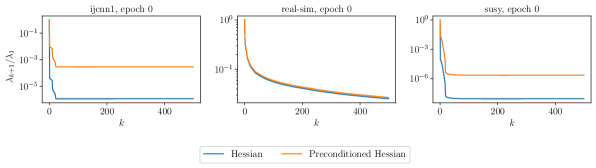
Figure 11: Normalized spectrum of the Hessian before and after preconditioning in $l_{2}$-regularized logistic regression.

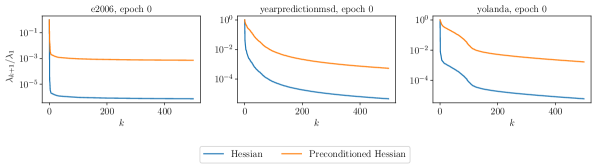
Figure 12: Normalized spectrum of the Hessian before and after preconditioning in ridge regression.

Figure 13: Spectrum of the Hessian at epoch $10$ before and after preconditioning in $l_{2}$-regularized logistic regression.

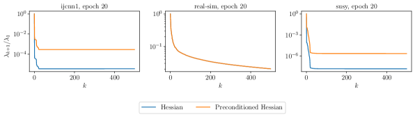
Figure 14: Spectrum of the Hessian at epoch $20$ before and after preconditioning in $l_{2}$-regularized logistic regression.

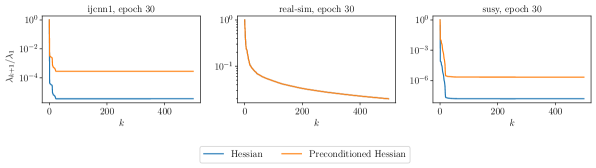
Figure 15: Spectrum of the Hessian at epoch $30$ before and after preconditioning in $l_{2}$-regularized logistic regression.

Appendix E Plots of test loss, training accuracy, and test accuracy

We present test loss, training accuracy, and test accuracy comparisons that were omitted from Sections 5.1, 5.2, and 5.3. Figures 16, 17, 18, and 19 display test loss/training accuracy/test accuracy plots corresponding to Section 5.1, where we compare SketchySGD to the competitor methods with their default hyperparameters. Figures 20, 21, 22, and 23 display test loss/training accuracy/test accuracy plots corresponding to Section 5.2, where we compare SketchySGD to the competitor methods with tuned hyperparameters. Figure 24 and Figure 25 display the test accuracies corresponding to Section 5.3, where we compare SketchySGD to competitor methods with both default and tuned hyperparameters on a large-scale version of the HIGGS dataset.

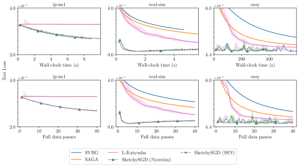
Figure 16: Test losses of competitor methods with default learning rates (SVRG, SAGA) and smoothness parameters (L-Katyusha) on $l_{2}$-regularized logistic regression.

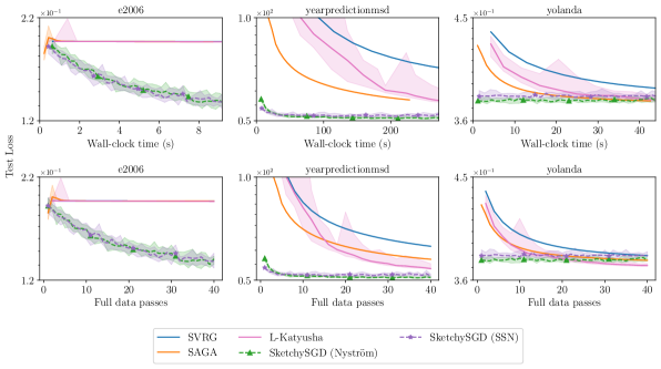
Figure 17: Test losses of competitor methods with default learning rates (SVRG, SAGA) and smoothness parameters (L-Katyusha) on ridge regression.

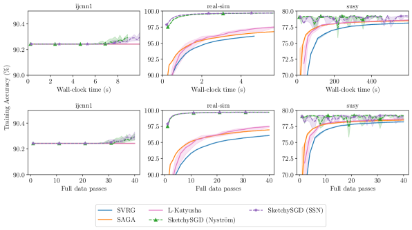
Figure 18: Training accuracies of competitor methods with default learning rates (SVRG, SAGA) and smoothness parameters (L-Katyusha) on $l_{2}$-regularized logistic regression.

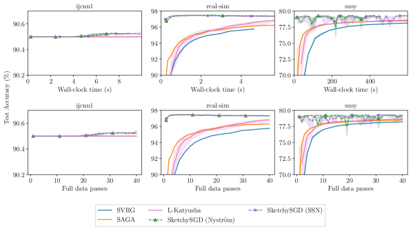
Figure 19: Test accuracies of competitor methods with default learning rates (SVRG, SAGA) and smoothness parameters (L-Katyusha) on $l_{2}$-regularized logistic regression.

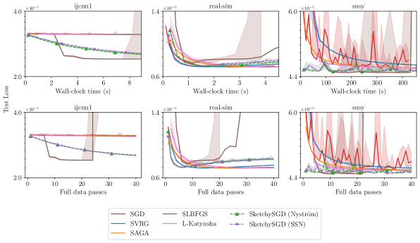
Figure 20: Test losses of competitor methods with tuned learning rates (SGD, SVRG, SAGA, SLBFGS) and smoothness parameters (L-Katyusha) on $l_{2}$-regularized logistic regression.

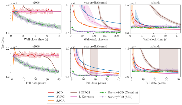
Figure 21: Test losses of competitor methods with tuned learning rates (SGD, SVRG, SAGA, SLBFGS) and smoothness parameters (L-Katyusha) on ridge regression.

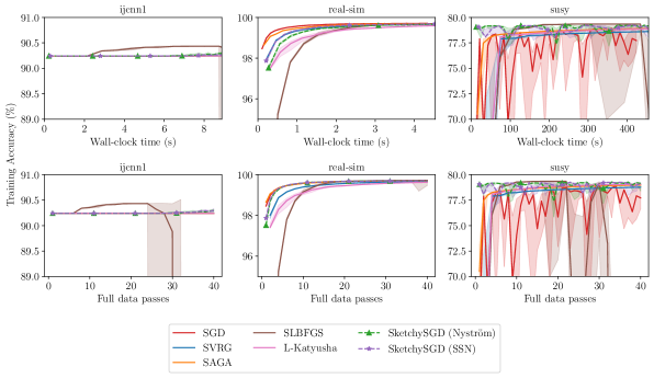
Figure 22: Training accuracies of competitor methods with tuned learning rates (SGD, SVRG, SAGA, SLBFGS) and smoothness parameters (L-Katyusha) on $l_{2}$-regularized logistic regression.

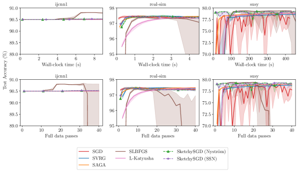
Figure 23: Test accuracies of competitor methods with tuned learning rates (SGD, SVRG, SAGA, SLBFGS) and smoothness parameters (L-Katyusha) on $l_{2}$-regularized logistic regression.

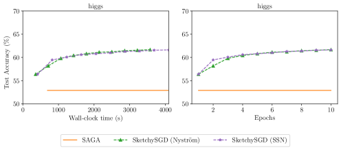
Figure 24: Comparison of test accuracies between SketchySGD and SAGA with default learning rate.

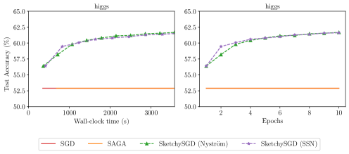
Figure 25: Comparison of test accuracies between SketchySGD, SGD and SAGA with tuned learning rates.

Appendix F Additional sensitivity experiments

We present additional plots that were omitted from the sensitivity study in the main text. Figure 26 shows how changing the rank $r$ impacts the performance of SketchySGD on the yolanda, ijcnn1, and susy datasets. We again observe that the effect of increasing the rank is correlated with the spectrum (Fig. 9) of each dataset. Both yolanda and yearpredictionmsd have similar patterns of spectral decay, and increasing the rank for yolanda leads to faster convergence to ball of noise, at the cost of more oscillation about the optimum. On the other hand, the spectra of ijcnn1 and susy are highly concentrated in the first singular value, just like E2006-tfidf and real-sim, and increasing the rank does not improve convergence. Fig. 27 demonstrates that adjusting the update frequency $u$ does not impact convergence on ridge regression problems.

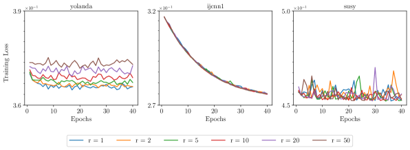
Figure 26: Sensitivity of SketchySGD to rank $r$.

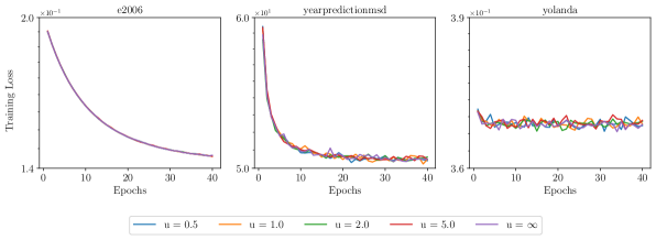
Figure 27: Sensitivity of SketchySGD to update frequency $u$.

References

- [1] https://www.csie.ntu.edu.tw/~cjlin/libsvmtools/datasets/binary.html#real-sim.
- [2] A. Agarwal, S. Negahban, and M. J. Wainwright, Fast global convergence of gradient methods for high-dimensional statistical recovery, The Annals of Statistics, (2012), pp. 2452–2482.
- [3] Z. Allen-Zhu, Katyusha: The first direct acceleration of stochastic gradient methods, Journal of Machine Learning Research, 18 (2018), pp. 1–51, http://jmlr.org/papers/v18/16-410.html.
- [4] P. Baldi, P. Sadowski, and D. Whiteson, Searching for exotic particles in high-energy physics with deep learning, Nature Communications, 5 (2014), https://doi.org/10.1038/ncomms5308, https://doi.org/10.1038/ncomms5308.
- [5] R. Bollapragada, R. H. Byrd, and J. Nocedal, Exact and inexact subsampled Newton methods for optimization, IMA Journal of Numerical Analysis, 39 (2019), pp. 545–578.
- [6] R. Bollapragada, J. Nocedal, D. Mudigere, H.-J. Shi, and P. T. P. Tang, A progressive batching l-bfgs method for machine learning, in International Conference on Machine Learning, PMLR, 2018, pp. 620–629.
- [7] S. P. Boyd and L. Vandenberghe, Convex optimization, Cambridge University Press, 2004.
- [8] R. H. Byrd, G. M. Chin, W. Neveitt, and J. Nocedal, On the use of stochastic Hessian information in optimization methods for machine learning, SIAM Journal on Optimization, 21 (2011), pp. 977–995.
- [9] E. Candes and B. Recht, Exact matrix completion via convex optimization, Communications of the ACM, 55 (2012), pp. 111–119.
- [10] E. Candes and J. Romberg, Sparsity and incoherence in compressive sampling, Inverse problems, 23 (2007), p. 969.
- [11] M. B. Cohen, S. Elder, C. Musco, C. Musco, and M. Persu, Dimensionality reduction for k-means clustering and low rank approximation, in Proceedings of the Forty-seventh Annual ACM Symposium on Theory of Computing, 2015, pp. 163–172.
- [12] A. Defazio, F. Bach, and S. Lacoste-Julien, SAGA: A fast incremental gradient method with support for non-strongly convex composite objectives, Advances in Neural Information Processing Systems, 27 (2014).
- [13] D. Dua and C. Graff, UCI machine learning repository, 2017, http://archive.ics.uci.edu/ml.
- [14] M. A. Erdogdu and A. Montanari, Convergence rates of sub-sampled Newton methods, Advances in Neural Information Processing Systems, 28 (2015).
- [15] Z. Frangella, J. A. Tropp, and M. Udell, Randomized Nyström preconditioning, Accepted at SIAM Journal on Matrix Analysis and Applications, (2022), https://arxiv.org/abs/2110.02820.
- [16] N. Gazagnadou, R. Gower, and J. Salmon, Optimal mini-batch and step sizes for saga, in International Conference on Machine Learning, PMLR, 2019, pp. 2142–2150.
- [17] R. Gower, D. Kovalev, F. Lieder, and P. Richtárik, RSN: Randomized subspace Newton, Advances in Neural Information Processing Systems, 32 (2019).
- [18] R. M. Gower, N. Loizou, X. Qian, A. Sailanbayev, E. Shulgin, and P. Richtárik, Sgd: General analysis and improved rates, in International Conference on Machine Learning, PMLR, 2019, pp. 5200–5209.
- [19] I. Guyon, L. Sun-Hosoya, M. Boullé, H. J. Escalante, S. Escalera, Z. Liu, D. Jajetic, B. Ray, M. Saeed, M. Sebag, A. Statnikov, W.-W. Tu, and E. Viegas, Analysis of the AutoML Challenge Series 2015–2018, Springer International Publishing, Cham, 2019, pp. 177–219, https://doi.org/10.1007/978-3-030-05318-5_10, https://doi.org/10.1007/978-3-030-05318-5_10.
- [20] N. Halko, P.-G. Martinsson, and J. A. Tropp, Finding structure with randomness: Probabilistic algorithms for constructing approximate matrix decompositions, SIAM Review, 53 (2011), pp. 217–288.
- [21] M. Hardt, B. Recht, and Y. Singer, Train faster, generalize better: Stability of stochastic gradient descent, in International Conference On Machine Learning, PMLR, 2016, pp. 1225–1234.
- [22] N. J. Higham, Accuracy and stability of numerical algorithms, SIAM, 2002.
- [23] R. Johnson and T. Zhang, Accelerating stochastic gradient descent using predictive variance reduction, Advances in Neural Information Processing Systems, 26 (2013).
- [24] S. Kogan, D. Levin, B. R. Routledge, J. S. Sagi, and N. A. Smith, Predicting risk from financial reports with regression, in Proceedings of Human Language Technologies: The 2009 Annual Conference of the North American Chapter of the Association for Computational Linguistics, NAACL ’09, USA, 2009, Association for Computational Linguistics, p. 272–280.
- [25] D. Kovalev, S. Horváth, and P. Richtárik, Don’t jump through hoops and remove those loops: SVRG and Katyusha are better without the outer loop, in Proceedings of the 31st International Conference on Algorithmic Learning Theory, A. Kontorovich and G. Neu, eds., vol. 117 of Proceedings of Machine Learning Research, PMLR, 08 Feb–11 Feb 2020, pp. 451–467, https://proceedings.mlr.press/v117/kovalev20a.html.
- [26] J. Kuczyński and H. Woźniakowski, Estimating the largest eigenvalue by the power and Lanczos algorithms with a random start, SIAM Journal on Matrix Analysis and Applications, 13 (1992), pp. 1094–1122.
- [27] J. Lacotte, Y. Wang, and M. Pilanci, Adaptive Newton sketch: linear-time optimization with quadratic convergence and effective hessian dimensionality, in International Conference on Machine Learning, PMLR, 2021, pp. 5926–5936.
- [28] K. Levenberg, A method for the solution of certain non-linear problems in least squares, Quarterly of Applied Mathematics, 2 (1944), pp. 164–168.
- [29] P.-L. Loh, On lower bounds for statistical learning theory, Entropy, 19 (2017), p. 617.
- [30] D. W. Marquardt, An algorithm for least-squares estimation of nonlinear parameters, Journal of the Society for Industrial and Applied Mathematics, 11 (1963), pp. 431–441.
- [31] P.-G. Martinsson and J. A. Tropp, Randomized numerical linear algebra: Foundations and algorithms, Acta Numerica, 29 (2020), pp. 403–572.
- [32] S. Mei, Y. Bai, and A. Montanari, The landscape of empirical risk for nonconvex losses, The Annals of Statistics, 46 (2018), pp. 2747–2774.
- [33] S. Mei and A. Montanari, The generalization error of random features regression: Precise asymptotics and the double descent curve, Communications on Pure and Applied Mathematics, 75 (2022), pp. 667–766, https://doi.org/https://doi.org/10.1002/cpa.22008, https://onlinelibrary.wiley.com/doi/abs/10.1002/cpa.22008, https://arxiv.org/abs/https://onlinelibrary.wiley.com/doi/pdf/10.1002/cpa.22008.
- [34] S. Y. Meng, S. Vaswani, I. H. Laradji, M. Schmidt, and S. Lacoste-Julien, Fast and furious convergence: Stochastic second order methods under interpolation, in International Conference on Artificial Intelligence and Statistics, PMLR, 2020, pp. 1375–1386.
- [35] P. Moritz, R. Nishihara, and M. Jordan, A linearly-convergent stochastic L-BFGS algorithm, in Artificial Intelligence and Statistics, PMLR, 2016, pp. 249–258.
- [36] E. Moulines and F. Bach, Non-asymptotic analysis of stochastic approximation algorithms for machine learning, Advances in Neural Information Processing Systems, 24 (2011).
- [37] A. Nemirovski, A. Juditsky, G. Lan, and A. Shapiro, Robust stochastic approximation approach to stochastic programming, SIAM Journal on optimization, 19 (2009), pp. 1574–1609.
- [38] J. Nocedal and S. J. Wright, Numerical optimization, Springer, 1999.
- [39] B. A. Pearlmutter, Fast exact multiplication by the Hessian, Neural Computation, 6 (1994), pp. 147–160.
- [40] F. Pedregosa, G. Varoquaux, A. Gramfort, V. Michel, B. Thirion, O. Grisel, M. Blondel, P. Prettenhofer, R. Weiss, V. Dubourg, et al., Scikit-learn: Machine learning in python, the Journal of machine Learning Research, 12 (2011), pp. 2825–2830.
- [41] A. Pensia, V. Jog, and P.-L. Loh, Generalization error bounds for noisy, iterative algorithms, in 2018 IEEE International Symposium on Information Theory (ISIT), IEEE, 2018, pp. 546–550.
- [42] M. Pilanci and M. J. Wainwright, Newton sketch: A near linear-time optimization algorithm with linear-quadratic convergence, SIAM Journal on Optimization, 27 (2017), pp. 205–245.
- [43] D. Prokhorov, IJCNN 2001 neural network competition, 2001.
- [44] A. Rahimi and B. Recht, Random features for large-scale kernel machines, Advances in Neural Information Processing Systems, 20 (2007).
- [45] H. Robbins and S. Monro, A stochastic approximation method, The Annals of Mathematical Statistics, (1951), pp. 400–407.
- [46] F. Roosta-Khorasani and M. W. Mahoney, Sub-sampled Newton methods, Mathematical Programming, 174 (2019), pp. 293–326.
- [47] T. Tong, C. Ma, and Y. Chi, Accelerating ill-conditioned low-rank matrix estimation via scaled gradient descent, The Journal of Machine Learning Research, 22 (2021), pp. 6639–6701.
- [48] J. A. Tropp, User-friendly tail bounds for sums of random matrices, Foundations of Computational Mathematics, 12 (2012), pp. 389–434.
- [49] J. A. Tropp, An introduction to matrix concentration inequalities, Foundations and Trends® in Machine Learning, 8 (2015), pp. 1–230.
- [50] J. A. Tropp, A. Yurtsever, M. Udell, and V. Cevher, Fixed-rank approximation of a positive-semidefinite matrix from streaming data, Advances in Neural Information Processing Systems, 30 (2017).
- [51] J. A. Tropp, A. Yurtsever, M. Udell, and V. Cevher, Practical sketching algorithms for low-rank matrix approximation, SIAM Journal on Matrix Analysis and Applications, 38 (2017), pp. 1454–1485.
- [52] M. J. Wainwright, High-dimensional statistics: A non-asymptotic viewpoint, vol. 48, Cambridge University Press, 2019.
- [53] D. P. Woodruff, Sketching as a tool for numerical linear algebra, Foundations and Trends® in Theoretical Computer Science, 10 (2014), pp. 1–157.
- [54] A. Xu and M. Raginsky, Information-theoretic analysis of generalization capability of learning algorithms, Advances in Neural Information Processing Systems, 30 (2017).
- [55] H. Ye, L. Luo, and Z. Zhang, Approximate Newton methods, Journal of Machine Learning Research, 22 (2021), pp. 1–41, http://jmlr.org/papers/v22/19-870.html.
- [56] S. Zhao, Z. Frangella, and M. Udell, NysADMM: faster composite convex optimization via low-rank approximation, in International Conference on Machine Learning, PMLR, 2022, pp. 26824–26840.