Environmental Toxicity Influences Disease Spread In Consumer Population

Abstract

The study of infectious disease has been of interest to ecologists since long. The initiation of epidemic and the long term disease dynamics are largely influenced by the nature of the underlying consumer (host)-resource dynamics. Ecological traits of such systems may be often modulated by toxins released in the environment due to ongoing anthropogenic activities. This, in addition to toxin-mediated alteration of epidemiological traits, has a significant impact on disease progression in ecosystems which is quite less studied. In order to address this, we consider a mathematical model of disease transmission in consumer population where multiple traits are affected by environmental toxins. Long term dynamics show that the level of environmental toxin determines disease persistence, and increasing toxin may even eradicate the disease in certain circumstances. Furthermore, our results demonstrate bistability between different ecosystem states and the possibility of an abrupt transition from disease-free coexistence to disease-induced extinction of consumers. Overall the results from this study will help us gain fundamental insights into disease propagation in natural ecosystems in the face of present anthropogenic changes.

1 Introduction

Environmental pollution and disease outbreaks are global threat to ecosystems in the present era of the Anthropocene (Lafferty et al, 2004; Van Bressem et al, 2009). Toxins released in the environment due to anthropogenic factors have long-drawn consequences on the ecosystem health (Huang et al, 2013, 2015; Garay-Narváez et al, 2013; Banerjee et al, 2021). The emergence of disease outbreaks in many ecosystems is also of utmost concern for ecologists (Lafferty and Kuris, 1999; Lafferty and Holt, 2003; Lafferty et al, 2004; Khan et al, 1990; Van Bressem et al, 2009). It is well known that environmental toxin can influence the impact of disease spread on ecosystem but the manner of it is not properly understood. Toxin can reduce the host immunity thus making them more susceptible which increases disease prevalence (Khan et al, 1990; Beck and Levander, 2000). Conversely, toxin may restrict movement and increase mortality of the infected host thus having a negative effect on disease spread. These synergistic and antagonistic effect makes it difficult to predict the impact of environmental toxin on long term disease dynamics in ecosystem thus highlighting the need for studies combining the two.

While toxin can affect disease transmission rate in multiple ways, it can also impact host-resource interaction which in turn can have significant impact on disease dynamics (Huang et al, 2015). In fact, the host-resource dynamics has received a lot of attention in the recent years in regard to disease progression in ecosystems (Hurtado et al, 2014; Hilker and Schmitz, 2008). In this context, it is important to note that even life history traits like growth rate and mortality of both resource and the host and the ingestion rate of the later can be influenced by environmental toxin. This affects abundance of the host population and thus disease prevalence. Majority of theoretical studies which tried to address the impact of chemical pollution on disease however neglected these effects (Sinha et al, 2010; Liu et al, 2012; Chauhan et al, 2015; Wang and Ma, 2004). Although a recent study by Banerjee et al (2019) on a Daphnia-algae-fungus system took into consideration some of these aspects, it has few shortcomings. These are mainly based on the fact that the toxic effect considered in this study are system specific which may not be reasonable when extrapolated to other contaminated systems in the environment.

For instance, Banerjee et al (2019) accounted for reduced disease transmission due to behavioural change of the host at toxic concentration of the pollutant. However, high environmental toxin may also lead to increased susceptibility of the host to disease (Coors and De Meester, 2008; Beck and Levander, 2000). This may be a result of toxin-induced immunity suppression which is ubiquitous in many epidemic scenarios (Coors and De Meester, 2008) and well demonstrated in plenty of experimental studies (de Swart et al, 1994; De Swart et al, 1996; Ross et al, 1996; Bogomolni et al, 2016). Especially, aquatic species and more specifically many marine mammals are known to be vulnerable to immuno-toxic contaminants (Ross, 2000, 2002; de Swart et al, 1994; De Swart et al, 1996; Ross et al, 1996; Bogomolni et al, 2016). For instance, harbor seals would be less immune if they fed on fish from the more polluted Baltic Sea and less susceptible in case their predation is associated with the less polluted Atlantic sea (Ross et al, 1996; de Swart et al, 1994). Furthermore, it has been pointed out earlier that environmental toxin should also have an effect on the carrying capacity as well (Freedman and Shukla, 1991), which was not taken into account by Banerjee et al (2019).

To address these gaps, we model disease progression in consumer population using the approach employed by earlier studies like Huang et al (2013, 2015); Thieme (2003). This implied the use of Beverton-Holt growth rate instead of conventional logistic formulation. Additionally, we consider toxin dependent increase in transmission and attempt to answer two interrelated questions: (1) How does environmental toxin influence the progression of disease? (2) How do the contamination and disease jointly shape the community composition of an ecosystem? First, we describe our model and toxin-mediated response functions in section 2. Also, we make our model parameters dimensionless and use a quasi-steady state approximation in this section to reduce model complexity. In section 3, we investigate the possible asymptotic states of our system with the help of bifurcation diagrams. Finally, our paper is summarized with a brief discussion in section 4.

2 Methods

2.1 Model description

We consider a consumer-resource model, where the consumer population is affected by an infectious disease (Hilker and Schmitz, 2008). Furthermore, we assume the ecological and epidemiological traits of the system are altered by environmental toxins. Let $x(t)$ and $y(t)$ be the concentration of the resource and the consumer biomass respectively. The consumer (host) population can be further segregated into susceptible, $S(t)$, and infected, $I(t)$, classes such that $S(t)+I(t)=y(t)$. It must be noted that, we have used the term ‘consumer’ and ‘host’ interchangeably through out the paper. Let $u(t)$ and $v(t)$ be the toxin body burden of the resource and consumer species respectively, which is defined as the ratio of the total toxin in a population to the total biomass concentration (Huang et al, 2015). Then the disease dynamics under the influence of environmental toxin can be described as below:

$$\frac{dx}{dt}=(\beta(x,u)-\mu_{1}(u))x-\frac{ax}{H+x}y\\$$ (1a)

$$\frac{dS}{dt}=e(v)\frac{ax}{H+x}y-\lambda(v)\frac{SI}{y}-\mu_{2}(v)S\\$$ (1b)

$$\frac{dI}{dt}=\lambda(v)\frac{SI}{y}-\mu_{2}(v)I-\eta I\\$$ (1c)

$$\frac{dy}{dt}=\frac{d(S+I)}{dt}=e(v)\frac{ax}{H+x}y-\mu_{2}(v)y-\eta I\\$$ (1d)

The first term on the right hand side of the equation 1(a) represents the net growth of the resource species in the absence of consumers, which is taken to be Beverton-Holt type (see Thieme (2003) for derivation of this term). Here, the reproduction and growth rate is represented by $\beta(x,u)=\displaystyle\frac{\alpha_{1}}{1+\alpha_{3}x}b(u)$, where $b(u)$ is the effect of toxin on the resource’s growth rate. The death rate is denoted by $\mu_{1}(u)$ which depends on the toxin body-burden of the resource, $u$. The second term is the biomass loss due to the predation by consumer and the functional response is taken to be Holling type-II, where $a$ is the maximum feeding rate and $H$ is the half-saturation constant. In equations 1(b-c), $e(v)$ is the food conversion efficiency, $\lambda(v)$ denotes the rate of disease transmission and $\mu_{2}(v)$ is the natural mortality rate of the consumer. All these parameters are assumed to be dependent on toxin body burden of the consumer, $v$. Infected consumers have an additional disease-induced death term (virulence), $\eta$. In our model, disease transmission is assumed to be frequency-dependent which implies that the per-capita force of infection increases with disease prevalence, $\displaystyle\frac{I}{y}$ (De Koeijer et al, 1998; Hilker and Schmitz, 2008).

For simplicity, we assume that the transmission rate is the only epidemiological trait which is toxin dependent. Also, we do not consider any recovery from the disease. For readers’ convenience, we used largely the same notations as in Hilker and Schmitz (2008) and Huang et al (2015) for parameters and state variables in this paper.

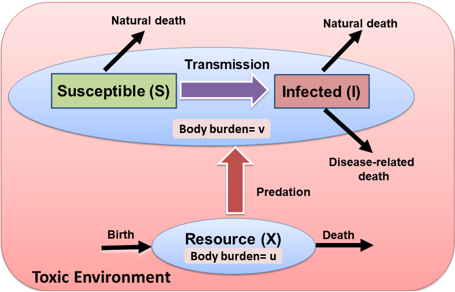
Figure 1: Schematic representation of our model. Resource growth is regulated by birth, death, and predation by the consumer. The consumer is divided into susceptible and infected classes. The system is under the influence of environmental toxin and the body burden of the resource and consumer are $u$ and $v$ respectively.

From the above equation 1, the rate of change of disease prevalence, $i(t)=\displaystyle\frac{I(t)}{y(t)}$, can be expressed as follows (see Appendix A for the derivation):

$$\frac{di}{dt}=\lambda(v)i(1-i)-e(v)\frac{ax}{H+x}i-\eta i(1-i)\\$$ (2)

Following Hilker and Schmitz (2008), we express the model (equation 1-2) in terms of $x$, $y$ and $i$, i.e., equation 1(a, d) and 2. This is particularly advantageous not only because it helps to remove the singularity in the disease transmission term when host population is zero, but also allows us to establish the cause of extinction of the host population. When host population becomes extinct due ecological factors, for example, high mortality rate the prevalence becomes zero. This is referred to as ecological extinction throughout the text. On the other hand, when epidemiological factors, for example, disease induced death is the underlying mechanism of host extinction, the prevalence remain strictly positive. In this case, which is referred to as epidemiological extinction henceforth, the positive prevalence signifies that the disease transmission occurs even when the population is very small (De Castro and Bolker, 2005; Hilker and Schmitz, 2008).

2.2 Modelling toxin accumulation

In order to incorporate the effect of toxin on the population dynamics of the interacting species, we must track the time evolution of the amount of the accumulated toxin concentration of the resource and consumer species ($U(t)$ and $V(t)$ respectively). Following Huang et al (2015), their dynamical equations can be written as:

$$\frac{dU}{dt}=a_{1}Tx-\sigma_{1}U-\mu_{1}(u)U-\frac{axy}{H+x}u\\$$ (3a)

$$\frac{dV}{dt}=a_{2}Ty-\sigma_{2}V+\frac{axy}{H+x}u-\mu_{2}(v)V-\eta iV\\$$ (3b)

Here, $T$ is the environmental toxicant concentration, $a_{i}$ and $\sigma_{i}$ ($i=1,2$) are the uptake and depuration coefficients of the toxin for resource and consumers respectively. The concentration of toxin accumulated in both the resource and consumer population are regulated by uptake from the environment and depuration due to metabolism. Additionally, toxin is lost due to natural death of both populations and disease induced death of the consumer. Predation by consumer also leads to transfer of toxin from the resource to itself resulting in biomagnification.

The body-burden of the resource and consumer population, already defined above, can thus be expressed as $u(t)=\displaystyle\frac{U(t)}{x(t)}$ and $v(t)=\displaystyle\frac{V(t)}{y(t)}$ respectively, the rate of change of which is given below (see Appendix A):

$$\frac{du}{dt}=a_{1}T-\sigma_{1}u-\beta(x,u)u$$ (4a)

$$\frac{dv}{dt}=a_{2}T-\sigma_{2}v+\frac{ax}{H+x}(u-ve(v))$$ (4b)

The system can now be fully described using the state variables, $x$, $y$ and $i$ together with the toxin body burdens $u$ and $v$. So the equations 1(a), 1(d), 2, and 4 are the equations of our interest for the remaining part of the paper.

2.3 Modeling responses due to the toxin

For analyzing our model, we describe specific forms of toxin body burden dependence for each of the concerned parameters mentioned in the earlier paragraphs.

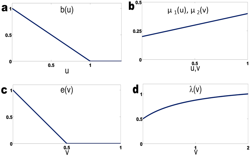
Figure 2: The responses of toxin body burden on parameters: (a) maximum reproduction rate, (b) mortality of the resource and consumer, (c) conversion efficiency of the consumer, (d) disease transmission rate.

Table 1: Variables and parameters description

Symbols	Unit	Description
Variables
$x$	$g/L$	resource density
$y$	$g/L$	consumer density
$S$	$g/L$	susceptible consumer density
$I$	$g/L$	infected consumer density
$U$	$\mu g/L$	concentration of the toxin in the resource
$V$	$\mu g/L$	concentration of the toxin in the consumer
$u$	$\mu g/g$	body burden of the resource
$v$	$\mu g/g$	body burden of the consumer
Parameters
$\alpha_{1}$	$day^{-1}$	maximum reproduction rate of the resource
$\alpha_{2}$	$g/\mu g$	effect of toxin on the growth of resource
$\alpha_{3}$	$L/g$	crowding effect of resource
$k_{1}$	$g/\mu g/day$	effect coefficient of the toxin on the resource mortality
$p$	$day^{-1}$	natural mortality of resource
$a$	$day^{-1}$	per-capita feeding rate
$H$	$g/L$	half saturation constant
$\beta_{1}$	-	reproduction efficiency of consumer
$\beta_{2}$	$g/\mu g$	effect of toxin on the reproduction of consumer
$m$	-	effect coefficient of the toxin on the transmission of the disease
$b$	$\mu g/g$	crowding effect of the consumer
$\lambda$	$day^{-1}$	disease transmission coefficient
$k_{2}$	$g/\mu g/day$	effect coefficient of the toxin on the consumer mortality
$\mu$	$day^{-1}$	natural mortality of consumer
$\eta$	$day^{-1}$	disease related mortality of consumer
$a_{1}$	$L/g/day$	uptake coefficient of resource
$\sigma_{1}$	$day^{-1}$	depuration coefficient of resource
$a_{2}$	$L/g/day$	uptake coefficient of consumer
$\sigma_{2}$	$day^{-1}$	depuration coefficient of consumer
$T$	$\mu g/L$	toxin concentration in the environment

The environmental toxicity is responsible for reducing the growth and reproduction of species in several ways. It can cause habitat degradation via changing chemical properties like salinity, acidity of marine surface and also hamper the growth of the primary producers like phytoplankton by changing the nutrient cycle (Cheevaporn and Menasveta, 2003; Roberts et al, 2013; Zeng et al, 2015). Thus we consider the effect of toxin on resource’s growth rate, $b(u)$, to be a monotonically decreasing function of the toxin body burden, $u$, i.e., $max(0,1-\alpha_{2}u)$ (Huang et al, 2013, 2015; Thieme, 2003). So the new maximum reproduction rate is given by $\alpha_{1}b(u)=\alpha_{1}max(0,1-\alpha_{2}u)$ (see Fig. 2a), which decreases linearly with $u$ upto the threshold value of $\displaystyle\frac{1}{\alpha_{2}}$, after which it becomes zero and so the resource stops growing. $\alpha_{2}$ is the effect coefficient of the toxin on the growth rate of the resource.

Furthermore, toxicants lead to decrease in the food conversion efficiency of the consumer (Huang et al, 2015; Garay-Narváez et al, 2013). We assume the consumer’s reproduction efficiency to be a linearly decreasing function of the consumer body burden, $v$, given by $e(v)=\beta_{1}max(0,1-\beta_{2}v)$ (see Fig. 2C), which becomes zero after the threshold value $\displaystyle\frac{1}{\beta_{2}}$. $\beta_{1}$ is the maximum conversion efficiency of the consumer and $\beta_{2}$ is the effect coefficient of the toxin on the consumer reproduction (Huang et al, 2015).

Environmental toxins decreases immunity of species against diseases (de Swart et al, 1994; De Swart et al, 1996; Ross et al, 1996) which increases the transmission rate. Keeping this in mind, we incorporate the effect of toxin on disease transmission. This is assumed to be a monotonically increasing function of the consumer body burden, $v$, (Wang et al, 2018) and is given by $\lambda(v)=(1+\displaystyle\frac{mv}{b+v})\lambda$ which eventually saturates to a limiting value $(1+m)\lambda$ (see Fig. 2D). Here, the parameter $m$ is the effect coefficient of the toxin on the transmission and $b$ is the crowding effect of the consumer, the reciprocal of which corresponds to how fast the transmission rate reaches to its limiting value.

All of the resource, susceptible and infected consumer are assumed to have toxin dependent morality term in addition to their natural mortality, which are linear functions of their toxin body burdens (Fig. 2b). The form of the mortality terms are $\mu_{1}(u)=p+k_{1}u$ and $\mu_{2}(v)=\mu+k_{2}v$ respectively, $k_{i},(i=1,2)$ being the effect coefficients of the toxin related mortality for resource and consumers respectively. See Table 1 for the description and units for all parameters and state variables mentioned so far.

2.4 Non-dimensionalization and quasi-steady state approximation

We introduce the following dimensionless variables and parameters:

$$\begin{split}\bar{x}&=\alpha_{3}x,\quad\bar{y}=\frac{a\alpha_{3}}{\alpha_{1}}y,\quad\bar{t}=\alpha_{1}t,\quad\bar{u}=\alpha_{2}u,\quad\bar{v}=\beta_{2}v,\\ &\bar{T}=\frac{\alpha_{2}a_{1}}{\sigma_{1}}T,\quad\bar{k_{1}}=\frac{k_{1}}{\alpha_{1}\alpha_{2}},\quad\bar{k_{2}}=\frac{k_{2}}{\alpha_{1}\beta_{2}},\quad\bar{p}=\frac{p}{\alpha_{1}},\quad\bar{h}=H\alpha_{3},\\ &\bar{\beta_{1}}=\frac{a\beta_{1}}{\alpha_{1}},\quad\bar{\beta_{2}}=\frac{a\beta_{2}}{\alpha_{2}\sigma_{1}},\quad\bar{\sigma_{2}}=\frac{\sigma_{2}}{\sigma_{1}},\quad\bar{\mu}=\frac{\mu}{\alpha_{1}},\quad\bar{\eta}=\frac{\eta}{\alpha_{1}},\\ &\bar{\lambda}=\frac{\lambda}{\alpha_{1}},\quad\bar{b}=b\beta_{2},\quad c=\frac{a_{2}\beta_{2}}{a_{1}\alpha_{2}},\quad\epsilon=\frac{\alpha_{1}}{\sigma_{1}}\end{split}$$

Substituting into the equations (1a, d, 2 and 4) and omitting the bars, we rewrite the system of equations as follows:

$$\frac{dx}{dt}=max(0,1-u)\frac{x}{1+x}-(k_{1}u+p)x-\frac{xy}{h+x}$$ (5a)

$$\frac{dy}{dt}=\beta_{1}max(0,1-v)\frac{xy}{H+x}-(k_{2}v+\mu)y-\eta iy$$ (5b)

$$\frac{di}{dt}=((1+\frac{mv}{b+v})\lambda-\eta)i(1-i)-\beta_{1}max(0,1-v)\frac{xi}{h+x}$$ (5c)

$$\epsilon\frac{du}{dt}=(T-u)-\epsilon max(0,1-u)\frac{u}{1+x}$$ (5d)

$$\epsilon\frac{dv}{dt}=cT-\sigma_{2}v+\frac{x}{h+x}(\beta_{2}u-\epsilon\beta_{1}vmax(0,1-v))$$ (5e)

The dynamics of the toxin body burden operates on a faster timescale compared to the species biomass growth. So the depuration rate of the toxin is higher compared to the reproduction of the resource. Our parameter $\epsilon$ is the ratio of the resource reproduction rate to the depuration rate of the toxin and so must be very small. So letting $\epsilon$ tends to zero, equation 5 (d, e) approaches to a quasi-steady state, which are given below:

$$u=T$$ (6a)

$$v=\frac{cT}{\sigma_{2}}+\frac{\beta_{2}T}{\sigma_{2}}\frac{x}{h+x}$$ (6b)

Substituting the quasi-steady states of the body burden equations, our simplified model becomes:

$$\frac{dx}{dt}=(\frac{max(0,1-u)}{1+x})x-(k_{1}u+p)x-\frac{xy}{h+x}$$ (7a)

$$\frac{dy}{dt}=\beta_{1}max(0,1-v)\frac{xy}{h+x}-(k_{2}v+\mu)y-\eta iy$$ (7b)

$$\frac{di}{dt}=[(1+\frac{mv}{b+v})\lambda-\eta]i(1-i)-\beta_{1}max(0,1-v)\frac{x}{h+x}i$$ (7c)

This model is further analyzed in the remaining part of the paper to study the role of environmental toxins in infectious disease dynamics in ecosystems.

2.5 Model calibration and analysis

For model analysis, all of the parameters are chosen from published literature (Huang et al, 2015; Hilker and Schmitz, 2008) which includes calibrated as well as hypothetical sets of values. In the absence of disease, our model reduces to that of Huang et al (2015) and in toxin free environment, it is equivalent to Hilker and Schmitz (2008). So the parameters related to toxin are chosen from the former while the disease related ones are chosen from the latter.

First, the mathematical proof of positive invariance and boundedness of the solutions of our model was carried out (see Appendix B). In order to explore the role of disease and toxicity on the steady state population dynamics, broad range of epidemiological parameters was chosen while keeping the ecological parameters fixed to compare the different dynamical scenarios with different level to toxicity and disease. We perform several one and two-parameter bifurcation diagrams to track the changes in the steady state population, with varying specified parameters through the MATCONT 6p11 (Dhooge et al, 2008) in MATLAB software.

3 Results

We use bifurcation analyses as a tool to address the questions outlined earlier. We also attempt to provide intuitive explanations of the different dynamical phenomena observed in the system. In the rest of the paper, $EQ_{1}$ denotes the disease-free coexistence equilibrium and $OSC_{1}$ denotes disease-free oscillations. The endemic equilibrium and population cycles are indicated as $EQ_{2}$ and $OSC_{2}$ respectively. Finally, the ecological extinction of the host is denoted by $CE_{1}$ and epidemiological extinction by $CE_{2}$.

3.1 Effect of toxin on disease dynamics

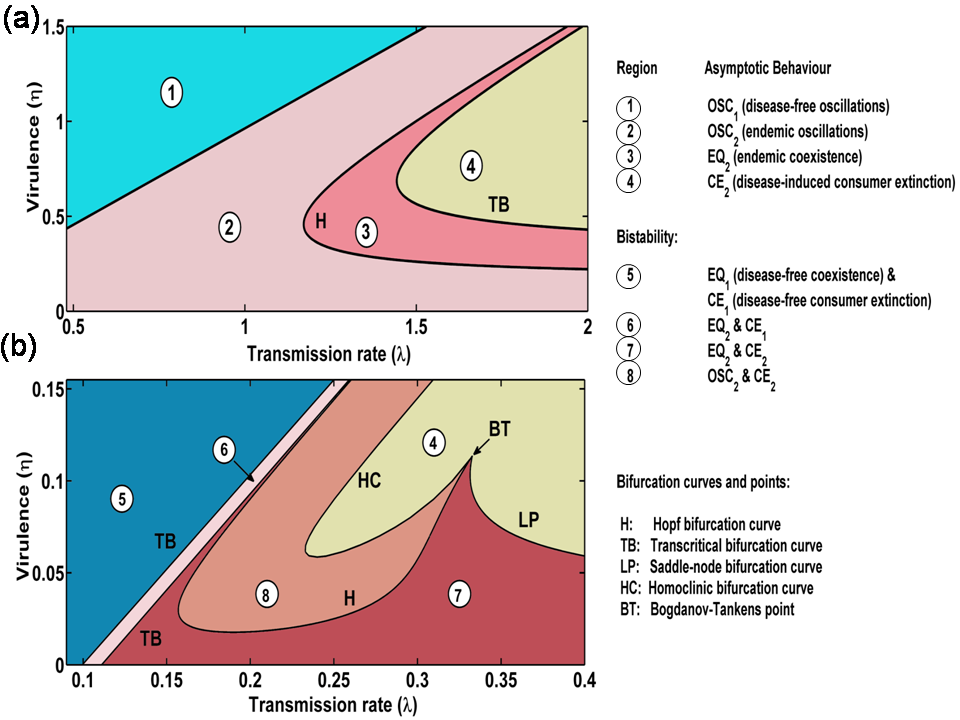
Figure 3: Two-parameter bifurcation diagram with respect to transmission rate ($\lambda$) and virulence ($\eta$) showcasing eight different dynamical regimes for environmental toxin levels (a) T=0.1, (b) T=0.1875. The other parameter values are $b_{1}=1,$ $b_{2}=4,$ $h=0.6,$ $m=0.1,$ $b=1,$ $c=1.5,$ $\sigma_{2}=1,$ $k_{1}=1,$ $p=0.1,$ $k_{2}=0.2,$ $\mu=0.02$.

The process of disease progression and elimination mainly depends on the two key epidemiological parameters, namely transmission rate ($\lambda$) and the virulence ($\eta$). We compare the dynamical behaviors of our system in the $\lambda-\eta$ plane for low and high contamination levels (see Fig. 3). When toxin is low ($T=0.1$, Fig. 3A), disease is introduced into the disease-free oscillations (region ①) with an increase in $\lambda$ leading to endemic cycles in region ②. This is followed by a Hopf bifurcation (H) as a result of which the cycle stabilizes in region ③. Further increase in $\lambda$ leads to epidemiological extinction of the consumers in region ④ by a transcritical bifurcation (TB). This behavior is qualitatively similar to the results demonstrated by Hilker and Schmitz (2008) who analyses the same model in the absence of toxicity. It is interesting to note that at higher virulence, $\eta$, disease establishes in the system only for reasonably high $\lambda$. This is because high virulence eliminates the infected host from the system resulting in eradication of the disease.

The dynamical behaviour of our system changed significantly with an increase in the toxin level (for $T=0.1875$, Fig. 3B). Now, when $\lambda$ is very low, the system exhibited bistability between two alternative stable states, $EQ_{1}$ and $CE_{1}$ (region ⑤). Further, moving along the $\lambda$ axis, the equilibrium $EQ_{1}$ alters its stability with $EQ_{2}$ resulting is persistence of disease in region ⑥. For low virulence ($\eta$), further increase in $\lambda$ will eventually shift the system dynamics to region ⑦ via a transcritical bifurcation (TB) where the system can switch between two alternative stable states, $EQ_{2}$ and $CE_{2}$. Here, depending on initial disease prevalence, the consumer survives with a partially infected population or will go to extinction (see 8). On the other hand, for higher virulence ($\eta$), on moving along the $\lambda$ axis, $EQ_{2}$ becomes unstable and endemic oscillation start through a Hopf bifurcation. So bistability between the states $OSC_{2}$ and $CE_{2}$ is observed in region ⑧. These oscillations can either become stable leading ‘bubbling effect’ as demonstrated in Fig. 4A-C or their amplitude increases with increasing $\lambda$ until it collapses suddenly to region ④ through a homoclinic bifurcation (see Fig. 4D-F). For the sake of clarity, we do not plot the consumer extinction equilibria ($CE_{1}$ and $CE_{2}$) in this figure.

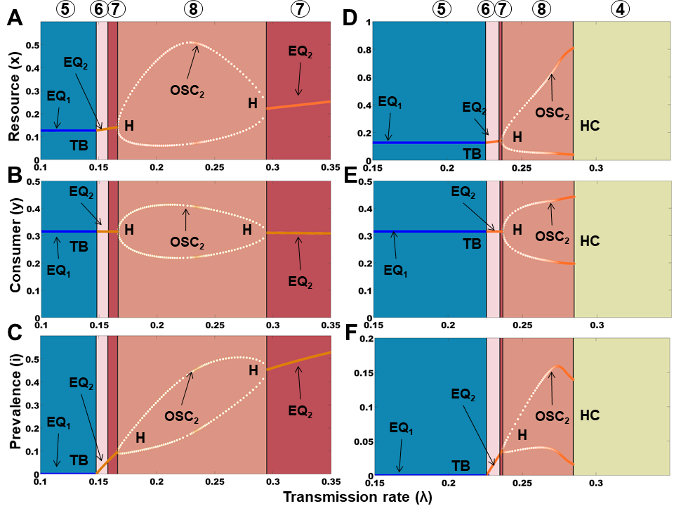
Figure 4: Effect of the transmission rate ($\lambda$) for virulence levels (A-C) $\eta=0.05$ and (D-F) $\eta=0.13$ under the high environmental toxin level ($T=0.1875$). Light blue and orange curves represent the disease-free ($EQ_{1}$) and endemic equilibrium ($EQ_{2}$) respectively. Orange circles represent the maximum and minimum population density of the endemic cycle ($OSC_{2}$). Parameter values are the same as in Fig. 3, and bifurcation points have their usual meaning as mentioned in Fig. 3.

3.2 Interplay between toxin and disease

To better understand the environmental toxin’s effect on the asymptotic resource and consumer dynamics, we plot one parameter bifurcation diagrams with respect to toxicity ($T$), for different transmission rates (e.g., for $\lambda=0.3$ and $0.5$) (see Fig. 5). When $\lambda=0.3$ (Fig. 5(A-C)), the system is in endemic oscillations ($OSC_{2}$) state for low level of toxin. Increasing toxicity introduces an alternative stable disease-free consumer extinction state $CE_{1}$ (Fig. 8) such that the consumer is unable to persist for low initial consumer population. Such toxicity induced Allee effect has been also demonstrated in the previous studies (Huang et al, 2015; Banerjee et al, 2019). The oscillations of the endemic cycle becomes stable ($EQ_{2}$) with increasing $T$ which is followed by a transcritical bifurcation leading to eradication of disease ($EQ_{1}$). Alternatively, the other equilibrium state $CE_{1}$, also undergoes transcritical bifurcation leading to disease induced consumer extinction, $CE_{2}$. Such dynamics leads to three more different types of bistability for changing toxin concentration as demonstrated in Fig. 5 (A-C). The bistability between $EQ_{1}$ and $CE_{2}$ is especially noteworthy as depending on the disease prevalence, either the system exists in disease free coexistence or if the disease persists, it leads to consumer extinction (see Fig. 7).

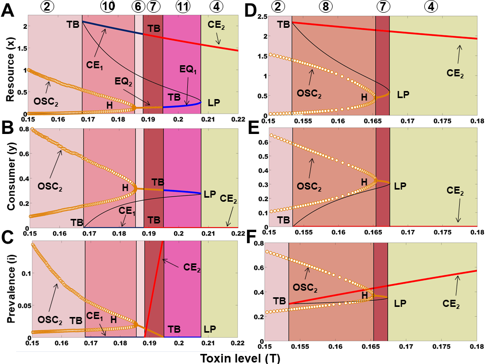
Figure 5: Effect of changing toxin concentration on the resource ($x$), the consumer ($y$), and prevalence ($i$) for different levels of disease transmission, (A-C) $\lambda=0.3$ and (D-F) $\lambda=0.5$. Parameter values are the same as Fig. 3. Orange and light blue curves indicate the endemic ($EQ_{2}$) and disease-free coexistence equilibrium ($EQ_{1}$) respectively. Orange circles represent the maximum and minimum population density of the endemic cycle ($OSC_{2})$. Deep blue and red curves indicate the ecological and epidemiological extinction of the consumers ($CE_{1}$ and $CE_{2}$, respectively). Black curves represent the unstable equilibrium branch.

Analysis reveals that on increasing toxin concentration, there may be an abrupt transition due to saddle-node bifurcation (LP), which leads to vanishing of the coexistence equilibrium thus rendering the consumer’s epidemiological extinction ($CE_{2}$) as the only stable state of the system. This transition is irreversible, i.e., once the system has passed the critical threshold (LP), decreasing toxin concentration can no longer return the system to the coexistence state. Further, it is important to note that the elimination of the disease from the endemic state ($EQ_{2}$) due to toxin may thus be a precursor to an irreversible extinction of the consumers. For the case of high transmission rate ($\lambda=0.5$, Fig. 5D-F), although increased toxin still leads to disease induced consumer extinction, the route to such extinction differs. For instance, there is no disease free coexistence in this case unlike the previous one.

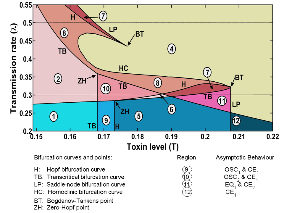
Figure 6: Two-parameter bifurcation diagram for environmental toxin level (T) and disease transmission rate ($\lambda$), demonstrating eleven different dynamical regimes. Regions ①-⑧ are as indicated in Fig. 3. Two black horizontal lines indicate the parameter values for which bifurcation diagrams in Fig. 5 are drawn. Here $\eta=0.2$ and other parameters are same as in Fig. 3.

The results so far points out the intricate relationship between toxin and disease dynamics. In order to achieve a holistic insight into how disease and toxicity jointly shape the community structure of our system, we carry out a two-parameter bifurcation analysis in the $T-\lambda$ plane (see Fig. 6). In this parametric plane, we identify all the different regions of asysmptotic behaviour exhibited in Fig. 3 (except ③). In addition, we find four new regions. Region ⑨ represents toxin induced bistability between disease free population cycle, $OSC_{1}$ and disease free consumer extinction, $CE_{1}$, which occurs only when transmission rate is very low. Very high toxin level lead to loss of such bistability and $CE_{1}$ is the only possible state as exhibited in region ⑫. At intermediate transmission rate, disease is introduced into the population cycles making it endemic oscillations, $OSC_{2}$, in region ⑩. Moving along increasing toxin axis, the cycle stabilizes and becomes disease free as system exhibits alternative stable states between disease free coexistence, $EQ_{1}$, and disease induced consumer extinction, $CE_{2}$, in region ⑪. An illustration of the equilibrium dynamics in different regions along the black horizontal line has been provided in the earlier Fig. 5.

Overall, it is observed that for lower values of transmission rate, $\lambda$, the system is in disease-free states represented by different shades of blue in Fig. 6. If we increase the toxin level, the system moves through the regions of different asymptotic behaviour to eventually consumer extinction. When transmission rate ($\lambda$) is high, the disease induced consumer extinction (region ④) occurs for much less toxin level, $T$.

4 Discussion

Disease and chemical pollution are important concerns for many ecosystems worldwide (Lafferty and Holt, 2003; Lafferty et al, 2004; Van Bressem et al, 2009) but studies integrating the two are rare. We used the approach prescribed by Huang et al (2013, 2015) to model the combined impact of environmental toxin and disease on consumer dynamics. We carried out bifurcation analysis, mainly with respect to environmental toxin parameter and disease related parameters to study the model behaviour. The results showcased in our study demonstrate the emergence of different dynamical scenarios and may help to contribute to our understanding of community ecology in the face of current anthropogenic changes.

To understand the impact of toxin on disease dynamics, we compare the behaviour of the system in the transmission-virulence plane for different toxin levels (see Fig. 3). With increasing toxin level, the disease may be established in the system for relatively lower transmission rate. This is expected because increasing environmental toxin increases disease transmission rate in our model. Furthermore, under low toxin concentration, when the system exhibits disease induced consumer extinction, it is the only stable state. On the contrary, when toxin level is high, if the initial disease prevalence is low, disease induced extinction may be avoided and the system may end up in either endemic coexistence equilibrium or population cycles depending on the transmission rate (see Fig. 8.B, C). The fact that disease causes this destabilization from equilibrium to cycles is noteworthy. This is because it is contrary to the stabilizing effect of disease as demonstrated in not only earlier studies (Hilker and Schmitz, 2008) but also when toxicity is low. The cycles collapse under high transmission rendering disease induced consumer extinction as the only possible stable state. Related interesting observation is that when virulence ($\eta$) is low, these cycles again stabilize on increasing transmission thus producing bubbling effect (see Fig. 4A-C).

A better understanding of the interaction between disease and toxin is achieved on studying the one parameter bifurcation diagram with respect to toxin and the system behaviour in the transmission-toxin parameter plane (Fig. 6). While increasing toxin amplifies the risk of disease as has been noted in the earlier paragraph, toxicity also eradicate the prevalent disease from the system. This is observed in region ⑪ where one of the bistable states, the endemic equilibrium, changes to disease free coexistence under increasing toxin (Fig.5.A, 6 ). Here, the consumer asymptotically may either become disease-free or extinct, depending on the initial prevalence level (Fig. 7.C). Abrupt disease-induced consumer extinction may also be observed. The toxin level at which such extinction occurs is higher when transmission is low which can be attributed to the synergistic effect of toxin on transmission in our model. Population oscillation and interestingly even disease-free coexistence can be precursor of such abrupt host extinction in the presence of toxin.

Toxicity introduces disease-free host extinction as an alternative stable state to the population cycles (Fig. 5.A-C). For instance, one can note the transition from $OSC_{1}$ to region ⑨ where both $OSC_{1}$ and $CE_{1}$ can exist and be stable (Fig. 7.B). Similarity in this behaviour to that observed by Huang et al (2015) is because of the fact that in the absence of disease our model reduces to that of the earlier one. In the presence of disease, this is translated to an interesting property whereby the prevalence of disease helps the host survive which would otherwise become extinct. However, for very high transmission, this is no more completely true as then the survival would depend on the initial prevalence of disease. Too high disease prevalence could then lead to disease-induced host extinction (see Fig. 6).

Overall our study throws light into the role of toxin in initiation and progression of an epidemic. Although the results presented here are significant in the context of disease dynamics, two key limitations of our model must be noted which could be addressed in future works. The effects of the toxin on disease induced host death rate were not considered in our analysis. Additionally, the infected population may recover from the disease, which is not considered in our system. Our work highlights the need to undertake more studies which will help comprehend the interaction between anthropogenic changes and disease in ecosystems and the non-linearity therein. Although management recommendation is not our direct aim but better fundamental understanding will pave the way for empirical validation and definitive actions.

Acknowledgments

Arnab and Amit acknowledges Senior Research Fellowship (file no: 09/093(0190)/2019-EMR-I and 09/093(0189)/2019-EMR-I) from Council of Scientific and Industrial Research (CSIR), India. Swarnendu was supported by the Visiting Scientist fellowship at Indian Statistical Institute, Kolkata during a part of this work. Swarnendu would also like to acknowledge his present funding under the Marie Skłodowska–Curie grant agreement 101025056 for the project ‘SpatialSAVE’.

Author contribution Arnab and Swarnendu conceived the idea; Arnab, Swarnendu, Sabyasachi refined it; Arnab and Swarnendu led the study and designed the simulations. Arnab and Amit programmed and ran the simulations. Arnab wrote the first draft of the manuscript. Swarnendu and Sabyasachi reviewed and edited the manuscript. All authors read and approved the final manuscript.

Declarations

Conflict of interest The authors declare no competing interests.

Appendix A Non-dimensionalisation and steady-state approximation

We first derive the equations of the disease prevalence and toxin body burdens of both the resource and consumers respectively as follows:

$$\begin{split}\frac{di}{dt}&=\frac{y\frac{dI}{dt}-I\frac{dy}{dt}}{y^{2}}\\ &=\frac{1}{y}\frac{dI}{dt}-\frac{I}{y}(\frac{y^{\prime}}{y})\\ &=\frac{1}{y}[(1+\frac{mv}{b+v})\frac{\lambda SI}{y}-(\mu+k_{2}v)I-\eta I]-i[e(v)\frac{ax}{H+x}-(\mu+k_{2}v)-\eta\frac{I}{y}]\\ &=[1+\frac{mv}{b+v}]\frac{\lambda Si}{y}-(\mu+k_{2}v)i-\eta i-i[e(v)\frac{ax}{H+x}-(\mu+k_{2}v)-\eta i]\\ &=[1+\frac{mv}{b+v}]\frac{\lambda i(1-i)y}{y}-e(v)\frac{ax}{H+x}i-\eta i(1-i)\\ &=[1+\frac{mv}{b+v}]\lambda i(1-i)-e(v)\frac{ax}{H+x}i-\eta i(1-i)\end{split}$$

$$\begin{split}\frac{du}{dt}&=\frac{d}{dt}(\frac{U}{x})\\ &=\frac{1}{x}\frac{dU}{dt}-\frac{U}{x}(\frac{1}{x}\frac{dx}{dt})\\ &=\frac{1}{x}(a_{1}Tx-\sigma_{1}U-\mu(u)U-\frac{axy}{H+x}u)-u(\beta(x,u)-\mu(u)-\frac{ay}{H+x})\\ &=a_{1}T-\sigma_{1}u-\beta(x,u)u\end{split}$$

$$\begin{split}\frac{dv}{dt}&=\frac{d}{dt}(\frac{V}{y})\\ &=\frac{1}{y}\frac{dV}{dt}-\frac{V}{y}(\frac{1}{y}\frac{dy}{dt})\\ &=\frac{1}{y}(a_{2}Ty-\sigma_{2}V+\frac{axy}{H+x}u-(\mu+k_{2}v)V-\eta\frac{I}{y}V)-v(e(v)\frac{ax}{H+x}-(\mu+k_{2}v)-\eta\frac{I}{y})\\ &=a_{2}T-\sigma_{2}v+\frac{ax}{H+x}(u-ve(v))\end{split}$$

Appendix B Proof of positivity and boundedness

The right hand side of the system (6 a-c) is continuously differentiable and locally Lipschitz in the first quadrant which implies the existence and uniqueness of solutions for the system in $R_{+}^{3}$. For positive invariance we rewrite the system as:

$$\frac{dX}{d\tau}=F(X)$$ (8)

Where $X=[x,y,z]^{T}\in R_{+}^{3}$ and $F(X)=[F_{1}(X),F_{2}(X),F_{3}(X)]^{T}$. The solutions of the system remain in the first quadrant for any non-negative initial condition for all $\tau\geq 0$, since ${F_{i}(X)}\mid_{X_{i}=0}\geq 0$, for all $X_{i}=0$ where $i=1,2,3$.

To proof positivity of the solutions of the system 6 a-c, we assume,

$$Z(t)=x+y+i$$

Differentiating $Z$ with respect to $t$ we get,

$$\begin{split}\frac{dZ}{dt}&=\frac{dx}{dt}+\frac{dy}{dt}+\frac{di}{dt}\\ &=(\frac{[1-u]_{+}x}{1+x})-(k_{1}u+p)x-\frac{xy}{h+x}+\beta_{1}\frac{[1-v]_{+}xy}{h+x}-(k_{2}v+\mu)y\\ &-\eta iy+[(1+\frac{mv}{b+v})\lambda-\eta]i(1-i)-\beta_{1}[1-v]_{+}\frac{x}{h+x}i\end{split}$$

Since $(\frac{[1-u]_{+}x}{1+x})<1$, $\beta_{1}\frac{[1-v]_{+}xy}{h+x}-\frac{xy}{h+x}\leq 0$ we can write,

$$\frac{dZ}{dt}<1-(k_{1}u+p)x-(k_{2}v+\mu)y-\eta iy+(1+\frac{mv}{b+v})\lambda i(1-i)-\eta i(1-i)-\beta_{1}[1-v]_{+}\frac{x}{h+x}i$$

As $\frac{v}{b+v}<1$, $k_{1}ux\geq 0$, $k_{2}vy\geq 0$, $\eta i(1-i)\geq 0$ and $\beta_{1}[1-v]_{+}\frac{x}{h+x}i\geq 0$,

$$\frac{dZ}{dt}\leq 1-px-\mu y+(1+m)\lambda i(1-i)$$

For an arbitrary positive real number $N$ we get,

$$\frac{dZ}{dt}+NZ<1-x(p-N)-y(\mu-N)+i((\lambda+m\lambda+N)-i(1+m)\lambda)$$

Let $N\leq min(p,\mu)$ and the maximum value of $i((\lambda+m\lambda+N)-i(1+m)\lambda)$ is $\frac{(\lambda+m\lambda+N)^{2}}{4(1+m)}$,

$$\frac{dZ}{dt}+NZ<1+\frac{(\lambda+m\lambda+N)^{2}}{4(1+m)}$$

Substituting $A=1+\frac{(\lambda+m\lambda+N)^{2}}{4(1+m)}$ we get,

$$\frac{dZ}{dt}+NZ<A$$

By diffrential inequality

$$0<Z(x,y,z)<\frac{A(1-exp(-Nt))}{N}+Z(x(0),y(0),z(0))exp(-Nt)$$

So for large values of t we have $0\leq Z\leq\frac{A}{N}$. Hence the solution of the system are bounded in the positive quadrant.

Appendix C Bistablity in the consumer-resource system

The system exhibits bistable dynamics for various parameter regimes (region ⑤-⑪). Fig. 7 demonstrates the bi-stable regimes for low level of disease transmission rate, whereas Fig. 8 for high level of transmission rate.

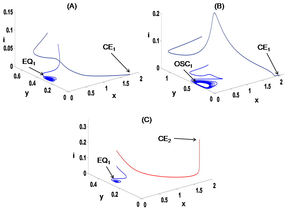
Figure 7: The solution trajectories for different bistability regions. (A) region ⑤; (parameters: $T=0.19$, $\lambda=0.25$), (B) region ⑨; (parameters: $T=0.17$, $\lambda=0.25$), (C) region ⑪; (parameters: $T=0.2$, $\lambda=0.3$). Bistability between disease-free coexistence and consumer extinction (disease-free or disease-induced) is seen.

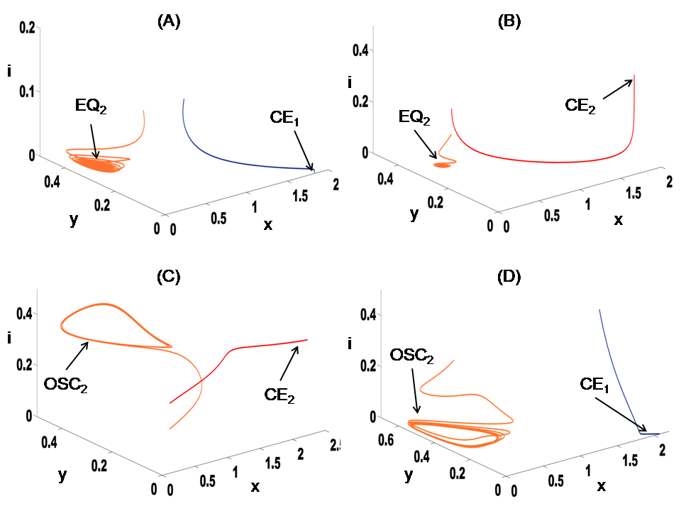
Figure 8: The solution trajectories for different bistability regions. (A) region ⑥; (parameters: $T=0.187$, $\lambda=0.3$), (B) region ⑦; (parameters: $T=0.2$, $\lambda=0.32$), (C) region ⑧; (parameters: $T=0.16$, $\lambda=0.5$), (C) region ⑩; (parameters: $T=0.17$, $\lambda=0.3$). Bistability between endemic coexistence and consumer extinction (disease-free or disease-induced) is seen.

References

- \bibcommenthead
- Banerjee et al (2019) Banerjee S, Sarkar RR, Chattopadhyay J (2019) Effect of copper contamination on zooplankton epidemics. Journal of theoretical biology 469:61–74
- Banerjee et al (2021) Banerjee S, Saha B, Rietkerk M, et al (2021) Chemical contamination-mediated regime shifts in planktonic systems. Theoretical Ecology 14(4):559–574
- Beck and Levander (2000) Beck MA, Levander OA (2000) Host nutritional status and its effect on a viral pathogen. The Journal of infectious diseases 182(Supplement_1):S93–S96
- Bogomolni et al (2016) Bogomolni A, Frasca S, Levin M, et al (2016) In vitro exposure of harbor seal immune cells to aroclor 1260 alters phocine distemper virus replication. Archives of environmental contamination and toxicology 70(1):121–132
- Chauhan et al (2015) Chauhan S, Bhatia SK, Gupta S (2015) Effect of pollution on dynamics of sir model with treatment. International Journal of Biomathematics 8(06):1550,083
- Cheevaporn and Menasveta (2003) Cheevaporn V, Menasveta P (2003) Water pollution and habitat degradation in the gulf of thailand. Marine Pollution Bulletin 47(1-6):43–51
- Coors and De Meester (2008) Coors A, De Meester L (2008) Synergistic, antagonistic and additive effects of multiple stressors: predation threat, parasitism and pesticide exposure in daphnia magna. Journal of Applied Ecology 45(6):1820–1828
- De Castro and Bolker (2005) De Castro F, Bolker B (2005) Mechanisms of disease-induced extinction. Ecology Letters 8(1):117–126
- De Koeijer et al (1998) De Koeijer A, Diekmann O, Reijnders P (1998) Modelling the spread of phocine distemper virus among harbour seals. Bulletin of mathematical biology 60(3):585–596
- De Swart et al (1996) De Swart RL, Ross PS, Vos JG, et al (1996) Impaired immunity in harbour seals (phoca vitulina) exposed to bioaccumulated environmental contaminants: review of a long-term feeding study. Environmental health perspectives 104(suppl 4):823–828
- Dhooge et al (2008) Dhooge A, Govaerts W, Kuznetsov YA, et al (2008) New features of the software matcont for bifurcation analysis of dynamical systems. Mathematical and Computer Modelling of Dynamical Systems 14(2):147–175
- Freedman and Shukla (1991) Freedman H, Shukla J (1991) Models for the effect of toxicant in single-species and predator-prey systems. Journal of Mathematical Biology 30(1):15–30
- Garay-Narváez et al (2013) Garay-Narváez L, Arim M, Flores JD, et al (2013) The more polluted the environment, the more important biodiversity is for food web stability. Oikos 122(8):1247–1253
- Hilker and Schmitz (2008) Hilker FM, Schmitz K (2008) Disease-induced stabilization of predator–prey oscillations. Journal of Theoretical Biology 255(3):299–306
- Huang et al (2013) Huang Q, Parshotam L, Wang H, et al (2013) A model for the impact of contaminants on fish population dynamics. Journal of theoretical biology 334:71–79
- Huang et al (2015) Huang Q, Wang H, Lewis MA (2015) The impact of environmental toxins on predator–prey dynamics. Journal of theoretical biology 378:12–30
- Hurtado et al (2014) Hurtado PJ, Hall SR, Ellner SP (2014) Infectious disease in consumer populations: dynamic consequences of resource-mediated transmission and infectiousness. Theoretical ecology 7(2):163–179
- Khan et al (1990) Khan R, et al (1990) Parasitism in marine fish after chronic exposure to petroleum hydrocarbons in the laboratory and to the exxon valdez oil spill. Bulletin of Environmental Contamination and Cytotoxicity 44(5):759–763
- Lafferty and Holt (2003) Lafferty KD, Holt RD (2003) How should environmental stress affect the population dynamics of disease? Ecology Letters 6(7):654–664
- Lafferty and Kuris (1999) Lafferty KD, Kuris AM (1999) How environmental stress affects the impacts of parasites. Limnology and Oceanography 44(3part2):925–931
- Lafferty et al (2004) Lafferty KD, Porter JW, Ford SE (2004) Are diseases increasing in the ocean? Annu Rev Ecol Evol Syst 35:31–54
- Liu et al (2012) Liu B, Duan Y, Luan S (2012) Dynamics of an si epidemic model with external effects in a polluted environment. Nonlinear Analysis: Real World Applications 13(1):27–38
- Roberts et al (2013) Roberts DA, Birchenough SN, Lewis C, et al (2013) Ocean acidification increases the toxicity of contaminated sediments. Global Change Biology 19(2):340–351
- Ross et al (1996) Ross P, De Swart R, Addison R, et al (1996) Contaminant-induced immunotoxicity in harbour seals: wildlife at risk? Toxicology 112(2):157–169
- Ross (2000) Ross PS (2000) Marine mammals as sentinels in ecological risk assessment. Human and Ecological Risk Assessment 6(1):29–46
- Ross (2002) Ross PS (2002) The role of immunotoxic environmental contaminants in facilitating the emergence of infectious diseases in marine mammals. Human and Ecological Risk Assessment: An International Journal 8(2):277–292
- Sinha et al (2010) Sinha S, Misra O, Dhar J (2010) A two species competition model under the simultaneous effect of toxicant and disease. Nonlinear Analysis: Real World Applications 11(2):1131–1142
- de Swart et al (1994) de Swart R, Ross P, Vedder L, et al (1994) Impairment of immune function in harbor seals (phoca vitulina) feeding on fish from polluted waters. Ambio 23(2):155–159
- Thieme (2003) Thieme HR (2003) Princeton series in theoretical and computational biology. In: Mathematics in Population Biology. Princeton University Press
- Van Bressem et al (2009) Van Bressem MF, Raga JA, Di Guardo G, et al (2009) Emerging infectious diseases in cetaceans worldwide and the possible role of environmental stressors. Diseases of aquatic organisms 86(2):143–157
- Wang and Ma (2004) Wang F, Ma Z (2004) Persistence and periodic orbits for an sis model in a polluted environment. Computers & Mathematics with Applications 47(4-5):779–792
- Wang et al (2018) Wang L, Jin Z, Wang H (2018) A switching model for the impact of toxins on the spread of infectious diseases. Journal of Mathematical Biology 77(4):1093–1115
- Zeng et al (2015) Zeng X, Chen X, Zhuang J (2015) The positive relationship between ocean acidification and pollution. Marine Pollution Bulletin 91(1):14–21