On the phase space of fourth-order fiber-orientation tensors

Abstract

Fiber-orientation tensors describe the relevant features of the fiber-orientation distribution compactly and are thus ubiquitous in injection-molding simulations and subsequent mechanical analyses. In engineering applications to date, the second-order fiber-orientation tensor is the basic quantity of interest, and the fourth-order fiber-orientation tensor is obtained via a closure approximation. Unfortunately, such a description limits the predictive capabilities of the modeling process significantly, because the wealth of possible fourth-order fiber-orientation tensors is not exploited by such closures, and the restriction to second-order fiber-orientation tensors implies artifacts. Closures based on the second-order fiber-orientation tensor face a fundamental problem - which fourth-order fiber-orientation tensors can be realized? In the literature, only necessary conditions for a fiber-orientation tensor to be connected to a fiber-orientation distribution are found. In this article, we show that the typically considered necessary conditions, positive semidefiniteness and a trace condition, are also sufficient for being a fourth-order fiber-orientation tensor in the physically relevant case of two and three spatial dimensions. Moreover, we show that these conditions are not sufficient in higher dimensions. The argument is based on convex duality and a celebrated theorem of D. Hilbert (1888) on the decomposability of positive and homogeneous polynomials of degree four. The result has numerous implications for modeling the flow and the resulting microstructures of fiber-reinforced composites, in particular for the effective elastic constants of such materials.
 
Keywords: Fiber-orientation tensor; Injection molding; Closure approximation; Effective elastic stiffness; Fiber-reinforced composite

1 Introduction

1.1 State of the art

Fiber-orientation tensors [1] date back to the far-reaching works [2, 3] and describe the relevant features of the fiber-orientation distribution of discontinuous fiber-reinforced composites. Within the virtual development and design process of such composites [4, 5, 1, 6], fiber-orientation tensors appear in material modeling [7, 8, 9, 10, 11, 12], microstructure generation [13, 14, 15, 16, 17, 18, 19], mold filling or flow simulations [20, 21, 22, 23, 24, 25] and the experimental computer tomography analysis [26, 27, 28]. This wide field of application motivates a detailed understanding of the mathematical properties of fiber-orientation tensors. Actually, the motivation and field of application is much more general, as fabric tensors and diffusion tensors share structural properties with fiber-orientation tensors. Fabric tensors [29, 7] share all characteristics with fiber-orientation tensors, except for a normalization constraint and are used in the field of porous materials. Diffusion tensors [30, 31, 32] also differ from fiber-orientation tensors only by a missing trace constraint and are used in medicine to describe the orientation of body tissues based on the diffusion motion of water molecules. This procedure is called diffusion-weighted magnetic resonance imaging (DW-MRI) [33, 34] and is, e.g., used on brain tissue to prevent strokes [35]. In particular, insights on the mathematical properties of fiber-orientation tensors might be transferred to diffusion tensors or fabric tensors.

The phase space of second-order fiber-orientation tensors is known [36, 37, 38, 39, 40], see the recent review [41]. A spectral decomposition is typically used to separate the structural features of a second-order fiber-orientation tensor, described by two independent eigenvalues with limited admissible parameter ranges, from the spatial alignment of this structural information in terms of a rotation or eigensystem. The limited structural variability of second-order fiber-orientation tensors is a critical ingredient for applications in process simulations [9, 10, 11, 5].

In contrast to the second-order case, the phase space of fourth-order fiber-orientation tensors is less well understood, a circumstance which motivated the work at hand. Algebraic properties of symmetry and normalization are agreed upon and discussed in the literature [42, 43, 44, 45, 46]. Bauer and Böhlke [41] developed an eigensystem-based parameterization of fourth-order fiber-orientation tensors combining the framework of irreducible tensors [47, 48, 49, 50, 51, 52, 53] with the work of Kanatani [2]. This parameterization ensures normalization as well as symmetry conditions automatically and separates second- and fourth-order data. Moreover, additional material-symmetry constraints may be taken into account in a natural way. Bauer and Böhlke [41] assume that positive semidefiniteness of the tensor is a sufficient condition to derive admissible parameter ranges, specifying the variety of fourth-order fiber-orientation tensors. This variety is presented for special cases motivated by material symmetry. The case of planar fourth-order fiber-orientation tensors and derived quantities is studied in successive papers [54, 55]. However, the necessary condition of positive semidefiniteness of the completely symmetric tensor is assumed to be sufficient. In section 2.3 of this work, sufficiency of this condition for the cases inspected by Bauer and Böhlke [41] is proven.

A scientific topic which is intimately connected to the question on the phase space of fourth-order fiber-orientation tensors, is fiber-orientation closure approximations. Such closure approximations [56, 22, 57, 37, 58, 59, 60, 61, 62] are tensor-valued functions which postulate a functional relationship between a given second-order fiber-orientation tensor and an unknown fourth-order fiber-orientation tensor [19]. Identifying the phase space of fourth-order fiber-orientation tensors is essential to solve a fundamental problem of closure approximations - which fourth- order fiber-orientation tensors can be realized?

1.2 Contributions

This work is divided into a basic and an applied part. In the first part, we provide a proof for a simple characterization for the phase space of realizable fourth-order fiber-orientation tensors in the physically relevant dimensions two and three. In case of second-order fiber-orientation tensors, such a characterization is straightforward to obtain. Any symmetric second-order tensor whose eigenvalues are non-negative and sum to unity represents such a fiber-orientation tensor. In case of fourth-order tensors, an educated guess gives that completely symmetric fourth-order tensors whose eigenvalues are non-negative and sum to unity should correspond to realizable fourth-order fiber-orientation tensors.
Our arguments are based on two key ingredients. First, we use convex duality theory, in the following form. Two closed convex cones coincide precisely if their dual cones coincide. For the case at hand, the dual cones are a bit simpler to work with. The second insight is based on the natural identification of completely symmetric tensors of order $k$ with homogeneous polynomials of degree $k$. Then, a celebrated theorem due to Hilbert [63] on the decomposability of a positive homogeneous polynomial of fourth degree into a sum of squares of homogeneous quadratic polynomials implies the claim. Interestingly, this theorem holds only in spatial dimensions two and three. For higher dimensions, this decomposability does not hold. In particular, the educated guess for characterizing the phase-space of fourth-order fiber-orientation tensors is actually false for spatial dimensions four and above. This fact shows that there are no "elementary", in particular dimension-independent, arguments for showing this characterization of the phase space to be valid.
As a by-product of our analysis, we show the equivalence of representations of fiber-orientation tensors in terms of integration, sums of monomials (rank-one tensors) and finite sums of monomials with non-negative weights summing to one, a consequence of Carathéodory’s theorem [64].
In the applied part, we investigate the geometry of the phase space of fourth-order fiber-orientation tensors via studying optimization problems on the latter. For this purpose, we consider suitable semidefinite programs, i.e., optimization problems posed on positive semidefinite matrices. Indeed, due to the characterization shown in the first part, we may identify a realizable fourth-oder fiber-orientation tensor with a positive semidefinite matrix in a suitable matrix representation (we use the Kelvin-Mandel notation).
Extreme states of the phase space of fourth-order fiber-orientation tensors are studied based on the parameterizations introduced in previous work [41], which separate second- and fourth-order data and enable to incorporate constraints on material symmetry easily. For fixed second-order information, we identify fourth-order data maximizing the projection onto a specified direction in two and three dimensions. Restricting the parameter space to orthotropic fourth-order information prohibits extreme projections into certain directions. These findings demonstrate the inherent limitations of closure approximations, as closed fourth-order information is automatically orthotropic. Due to the close connection to effective elastic properties, corresponding limitations of the effective stiffnesses become clear, as well.

This paper is organized as follows. After recapitulating basic properties of fiber-orientation tensors and their representation by finite sums, see section 2.1, we specify a set of fiber-orientation tensor candidates in section 2.2. In section 2.3, we establish sufficiency of the conditions these candidates fulfill for tensor order four and dimensions two and three, leading to applications in section 3. In section 3.1, optimization on fiber-orientation tensors is identified as semidefinite programming. Consequences of material symmetry constraints, introduced in section 3.2, on the problem of extreme fourth-order information, defined in section 3.3, are presented in sections 3.4 and 3.5 for dimensions three and two.

2 Realizability of fourth-order fiber-orientation tensors

2.1 Fiber-orientation tensors

A non-polar fiber-orientation distribution is given by a probability measure $\mu$ on the unit sphere

$$S^{d-1}=\left\{p\in\mathds{R}^{d}\,\middle|\,\|p\|=1\right\}$$ (2.1)

in $d$ spatial dimensions which is invariant w.r.t. the involution $p\mapsto-p$ on the unit sphere. This definition includes continuous fiber-orientation distributions, described by non-negative and suitably normalized functions $\varphi$ via the measure

$${\mu=\varphi\,dA}$$ (2.2)

in terms of the usual surface measure $dA$ on the unit sphere. Moreover, discrete fiber-orientation states, described in terms of $N$ vectors $p_{i}\in S^{d-1}$ are included via the formulation

$$\mu=\frac{1}{2N}\sum_{i=1}^{N}\left(\delta_{p_{i}}+\delta_{-p_{i}}\right),$$ (2.3)

where $\delta_{p}$ denotes the Dirac measure concentrated on the point $p$.
As working with such measures may be cumbersome, Advani-Tucker [3] (compare also Kanatani [2]) introduced the so-called fiber-orientation tensors $A^{(k)}$ of order $k$, where $k$ denotes a non-negative integer, via the definition

$$A^{(k)}=\int_{S^{d-1}}p^{\otimes k}\,d\mu(p)$$ (2.4)

in terms of the $k$-fold outer tensor product $p^{\otimes k}$ of the unit vector $p$, integrated over the unit sphere. The fiber-orientation tensors have the following properties.

1. The fiber-orientation tensors are completely symmetric, i.e., the identity

   $$A^{(k)}_{i_{1}\,i_{2}\,\ldots\,i_{k}}=A^{(k)}_{i_{\sigma(1)}\,i_{\sigma(2)}\,\ldots\,i_{\sigma(k)}},\quad i_{j}\in\{1,\ldots,d\},\quad j\in\{1,\ldots,k\}$$ (2.5)

   holds for the components of the tensor $A^{(k)}$ and any permutation $\sigma$ of the index set $\{1,\ldots,k\}$. Denoting by $\textrm{Sym}_{d}(k)$ the vector space of completely symmetric $k$-th order tensors in $d$ dimensions, the condition (2.5) is equivalent to the inclusion $A^{(k)}\in{\textrm{Sym}_{k}(d)}$.

2. For odd order $k$, the fiber-orientation tensors vanish.

3. The fiber-orientation tensor $A^{(k)}$ is positive semidefinite in the sense that

   $$A^{(k)}\cdot^{k}q^{\otimes k}\geq 0$$ (2.6)

   holds for all vectors $q\in\mathds{R}^{d}$ and the $k$-fold index contraction $\cdot^{k}$ of tensors.

4. Double contraction with the $d\times d$-identity $\operatorname{\textrm{Id}}$ recovers the fiber-orientation tensor of two orders lower

   $$A^{(k+2)}:\operatorname{\textrm{Id}}=A^{(k)},\quad k=0,1,2,\ldots$$ (2.7)

5. The zeroth-order fiber-orientation tensor is unity, i.e., the equation

   $$A^{(0)}=1$$ (2.8)

   holds.

6. Any fixed fiber-orientation tensor $A^{(k)}$ of even order may be written as a finite sum

   $$A^{(k)}=\sum_{i=1}^{r}w_{i}\,q_{i}^{\otimes k}$$ (2.9)

   with appropriate non-negative weights $w_{i}$ which sum to unity, directions $q_{i}\in S^{d-1}$ and a non-negative integer $r$ not exceeding ${{k+d-1}\choose{d-1}}$.

These properties 1.-5. are elementary to verify and well-known [3]. We provide a derivation of property 6. in the Appendix A. Property 6. permits us to restrict to finite sums (2.9) when considering fiber-orientation tensors of fixed order. In particular, it is not necessary to resort to the general integration-based definition (2.4).

2.2 Fiber-orientation tensor candidates

The work at hand is specifically concerned with fourth-order fiber-orientation tensors $A^{(4)}\equiv\mathds{A}$. More precisely, we are interested in the set of realizable fourth-order fiber-orientation tensors

$$\texttt{A}(d)=\left\{\mathds{A}\in\textrm{Sym}_{4}(d)\,\middle|\,\mathds{A}=\int_{S^{d-1}}p^{\otimes 4}\,d\mu(p)\quad\text{for a fiber-orientation distribution}\quad\mu\right\}.$$ (2.10)

By Property 6. of the previous section, the set $\texttt{A}(d)$ may be rewritten in the form

$$\texttt{A}(d)=\left\{\mathds{A}=\sum_{i=1}^{r}\mu_{i}\,p_{i}^{\otimes 4}\,\middle|\,r>0,\quad{\mu_{i}>0}\quad\text{with}\quad\sum_{i=1}^{r}\mu_{i}=1,\quad p_{i}\in S^{d-1}\right\},$$ (2.11)

which is more convenient from the mathematical point of view.
The fundamental question we wish to answer in this work is the following. Suppose a fourth-order tensor $\mathds{A}$ is given - under which (easy to verify) conditions can it be represented in the form (2.11)? Here, the non-negativity of the weights is crucial. Indeed, every completely symmetric $k$-th order tensor can be written as a linear combination of monomials [65, Lemma 4.2], i.e., with both positive and negative weights.
Elements $\mathds{A}\in\texttt{A}(d)$ are completely symmetric (2.5), positive semidefinite on quartics (2.6)

$$\mathds{A}::q^{\otimes 4}\geq 0\quad\text{for all}\quad q\in\mathds{R}^{d},$$ (2.12)

and satisfy the trace-conditions (2.7) as well as (2.8). Here, the operator $::$ stands for a fourth-fold contraction, and gives rise to an inner product on the space $\textrm{Sym}_{4}(d)$ of completely symmetric fourth-order tensors.
However, it is readily seen that fiber-orientation tensors $\mathds{A}\in\texttt{A}(d)$ satisfy a non-negativity condition which is stronger than the condition (2.12). More precisely, for any tensor $\mathds{A}\in\texttt{A}(d)$, the inequality

$$S:\mathds{A}:S\geq 0\quad\text{holds for all}\quad S\in\textrm{Sym}_{2}(d),$$ (2.13)

i.e., symmetric second-order tensors $S$ in dimension $d$. Indeed, in view of the representation (2.11), we observe

$$S:\mathds{A}:S=\sum_{i=1}^{r}\mu_{i}\,S:p_{i}^{\otimes 4}:S=\sum_{i=1}^{r}\mu_{i}\,\left(S:p_{i}^{\otimes 2}\right)^{2}\geq 0$$ (2.14)

for any $S\in\textrm{Sym}_{2}(d)$ due to the non-negativity of the weights $\mu_{i}$. Please notice that the condition (2.13) is stronger than the condition (2.12) as the special symmetric tensor $S=q\otimes q$ may be chosen in the condition (2.13). Moreover, the condition (2.13) is equivalent to the positive semidefiniteness of the tensor $\mathds{A}$, considered as a linear operator

$$\textrm{Sym}_{2}(d)\rightarrow\textrm{Sym}_{2}(d),\quad S\mapsto\mathds{A}:S,$$ (2.15)

on the vector space $\textrm{Sym}_{2}(d)$, endowed with the inner product $(S,T)\mapsto S:T$.
In the literature, the following set is typically considered [41]

$$\texttt{Cand}(d)=\left\{\mathds{A}\in\textrm{Sym}_{4}(d)\,\middle|\,\mathds{A}\quad\text{{is positive semidefinite} \eqref{sec:fot_nec_nonnegative_twofold}},\quad\operatorname{\textrm{Id}}:\mathds{A}:\operatorname{\textrm{Id}}=1\right\}$$ (2.16)

to consist of reasonable candidates for fiber-orientation tensors.
The set (2.16) is much easier to work with in practice than the original set $\texttt{A}(d)$. Indeed, suppose a candidate tensor $\mathds{A}$ is given. Then, it is elementary to examine its complete symmetry. Moreover, the non-negativity condition (2.13) and the normalization requirement $\mathds{A}::\operatorname{\textrm{Id}}\otimes\operatorname{\textrm{Id}}=1$ are assessed via an eigendecomposition of the fourth-order tensor $\mathds{A}$, e.g., conveniently computed in an orthogonal basis like the Kelvin-Mandel representation [66, 67]. Indeed, both conditions are satisfied precisely if the eigenvalues are non-negative and sum to unity.
In contrast, the defining condition of realizable fiber-orientation tensors (2.11) is much harder to check, as it involves a canonical decomposition problem with non-negativity constraints, which is known to be non-trivial [65].
Properties 1., 4. and 5. of fiber-orientation tensors, listed in the previous section 2.1, imply all defining conditions of the set $\texttt{Cand}(d)$. Moreover, we just established the positive semidefiniteness condition (2.13). Thus, the inclusion of sets

$$\texttt{A}(d)\subseteq\texttt{Cand}(d)$$ (2.17)

holds. The impending question remains whether the set inclusion (2.17) is strict or not, i.e., whether every element $\mathds{A}\in\texttt{Cand}(d)$ is also realizable, i.e., $\mathds{A}\in\texttt{A}(d)$ holds.

2.3 On sufficiency of conditions

The purpose of this section is to check when the inverse direction of the inclusion (2.17)

$$\texttt{Cand}(d)\subseteq\texttt{A}(d)$$ (2.18)

holds. It will turn out that this is true for spatial dimensions $d\leq 3$ and false for dimension $d\geq 4$.
Central to our arguments is the auxiliary set

$$\texttt{Q}(d)=\left\{\mathds{A}\in\textrm{Sym}_{4}(d)\,\middle|\,\mathds{A}=\sum_{i=1}^{r}\mu_{i}\,p_{i}^{\otimes 4},\quad\mu_{i}\in\mathds{R}_{\geq 0},\quad p_{i}\in S^{d-1},\quad r\in\mathds{N}_{0}\right\}$$ (2.19)

of sums of fourth-order tensor-powers of vectors with non-negative weights and the set of tensors

$$\texttt{N}(d)=\left\{\mathds{A}\in\textrm{Sym}_{4}(d)\,\middle|\,S:\mathds{A}:S\geq 0\quad\text{for all}\quad S\in\textrm{Sym}_{2}(d)\right\}$$ (2.20)

which are completely symmetric and positive semidefinite (2.13). Notice that, in contrast to the definition (2.11) of the set $\texttt{A}(d)$, we use non-negative weights in the definition (2.19) instead of positive weights to include the zero tensor in the set $\texttt{Q}(d)$. This inclusion is necessary for the set $\texttt{Q}(d)$ to be closed.
The intersection conditions

$$\texttt{A}(d)=\texttt{Q}(d)\cap\left\{\mathds{A}\in\textrm{Sym}_{4}(d)\,\middle|\,\operatorname{\textrm{Id}}:\mathds{A}:\operatorname{\textrm{Id}}=1\right\}$$ (2.21)

and

$$\texttt{Cand}(d)=\texttt{N}(d)\cap\left\{\mathds{A}\in\textrm{Sym}_{4}(d)\,\middle|\,\operatorname{\textrm{Id}}:\mathds{A}:\operatorname{\textrm{Id}}=1\right\}$$ (2.22)

hold. Thus, we have the implication

$$\text{if}\quad\texttt{Q}(d)=\texttt{N}(d)\quad\text{holds, then}\quad\texttt{A}(d)=\texttt{Cand}(d)\quad\text{follows.}$$ (2.23)

In particular, the fiber-orientation realization problem (2.18) may be studied in terms of the sets (2.19) and (2.20). Both sets are closed convex cones, i.e., they are closed, convex and invariant under the action $\mathds{A}\mapsto\lambda\mathds{A}$ for $\lambda\geq 0$. For the set $\texttt{N}(d)$, the definition (2.20) immediately implies that it is a closed convex cone. Indeed, inequality constraints involving continuous functions lead to closed sets in finite dimensions, and the representation $S:\mathds{A}:S=\mathds{A}::{\left(S\otimes S\right)}$ recasts the set (2.20) as an intersection of half spaces through zero. As the intersection of (a family of) convex cones is a convex cone, we see that the set (2.20) is a convex cone.
For the set $\texttt{Q}(d)$, the definition (2.19) implies that the set is a convex cone. The closedness is a consequence of Carathéodory’s theorem [64], as detailed in the Appendix A. Indeed, as a consequence of this theorem, we may assume that no more than $r_{\max}={{k+d-1}\choose{d-1}}$ terms enter in the definition (2.19). Suppose a sequence $\left(\mathds{A}_{k}\right)$ of elements in $\texttt{Q}(d)$ converges to some $\mathds{A}\in\textrm{Sym}_{4}(d)$. Let us write

$$\mathds{A}_{k}=\sum_{i=1}^{r_{\texttt{max}}}\mu_{i,k}\,p_{i,k}^{\otimes 4},\quad\mu_{i,k}\geq 0,\quad p_{i,k}\in S^{d-1}.$$ (2.24)

We observe

$$\sum_{i=1}^{r_{\texttt{max}}}\mu_{i,k}=\operatorname{\textrm{Id}}:\mathds{A}_{k}:\operatorname{\textrm{Id}}\rightarrow\operatorname{\textrm{Id}}:\mathds{A}:\operatorname{\textrm{Id}}\quad\text{as}\quad k\rightarrow\infty.$$ (2.25)

Thus, there is a uniform bound $C$ on the coefficients $\mu_{i,k}$. As the sets $[0,C]$ and $S^{d-1}$ are compact, we may extract a subsequence (not relabeled), s.t.

$$\mu_{i,k}\rightarrow\mu_{i}\quad\text{and}\quad p_{i,k}\rightarrow p_{i}\quad\text{as}\quad k\rightarrow\infty$$ (2.26)

for suitable $\mu_{i}\in[0,C]$ and $p_{i}\in S^{d-1}$. Due to the uniqueness of limits, we obtain the representation

$$\mathds{A}=\sum_{i=1}^{r_{\texttt{max}}}\mu_{i}\,p^{\otimes 4},\quad\text{i.e.},\quad\mathds{A}\in\texttt{Q}(d).$$ (2.27)

Hence, the set $\texttt{Q}(d)$ is closed.
For any set $C\subseteq\mathds{R}^{m}$ with inner product $\langle\cdot,\cdot\rangle$, the dual cone $C^{*}\subseteq\mathds{R}^{m}$ is defined by the relation

$$C^{*}=\left\{z\in\mathds{R}^{m}\,\middle|\,\langle z,x\rangle\geq 0\quad\text{for all}\quad x\in C\right\}.$$ (2.28)

It is immediate to see that the set $C^{*}$ does indeed define a closed convex cone. If, moreover, the original set $C$ was a closed convex cone to start with, the dual cone of the dual cone coincides with the original set

$$C^{**}=C.$$ (2.29)

This assertion is a consequence of convex duality theory [68].
As we identified the sets $\texttt{Q}(d)$ and $\texttt{N}(d)$ as closed convex cones, the equivalence

$$\texttt{Q}(d)=\texttt{N}(d)\quad\text{precisely if}\quad\texttt{Q}(d)^{*}=\texttt{N}(d)^{*}$$ (2.30)

follows directly, where we fix the inner product

$$\langle\mathds{A},\mathds{B}\rangle=\mathds{A}::\mathds{B},\quad\mathds{A},\mathds{B}\in\textrm{Sym}_{4}(d).$$ (2.31)

For this assertion to be useful, it is necessary to identify the dual cones explicitly. We have

$$\texttt{Q}(d)^{*}=\left\{\mathds{B}\in\textrm{Sym}_{4}(d)\,\middle|\,\mathds{B}::q^{\otimes k}\geq 0\quad\text{for all}\quad q\in\mathds{R}^{d}\right\}.$$ (2.32)

Indeed, the inclusion $\subseteq$ follows from the definition of the dual cone (2.28)

$$\texttt{Q}(d)^{*}=\left\{\mathds{B}\in\textrm{Sym}_{4}(d)\,\middle|\,\mathds{A}::\mathds{B}\geq 0\quad\text{for all}\quad\mathds{A}\in\texttt{Q}(d)\right\}$$ (2.33)

by selecting $\mathds{A}=p^{\otimes 4}$ as an element of $\texttt{Q}(d)$. The inclusion $\supseteq$ follows by considering

$$\mathds{A}::\mathds{B}=\sum_{i=1}^{r}\mu_{i}\,\underbrace{B::p_{i}^{\otimes 4}}_{\geq 0}\geq 0\quad\text{for}\quad\mathds{A}\in\texttt{Q}(d).$$ (2.34)

With a completely analogous argument, we obtain

$$\texttt{N}(d)^{*}=\left\{\mathds{B}\in\textrm{Sym}_{4}(d)\,\middle|\,\mathds{B}=\sum_{i=1}^{r}\texttt{sym}(S_{i}\otimes S_{i}),\quad S_{i}\in\textrm{Sym}_{2}(d)\right\},$$ (2.35)

where sym refers to the complete symmetrization of all indices. To study when the sets $\texttt{Q}(d)^{*}$ and $\texttt{N}(d)^{*}$ coincide, we use the identification of completely symmetric tensors with homogeneous polynomials. More precisely, for any tensor $\mathds{B}\in\textrm{Sym}_{4}(d)$, the function

$$P_{\mathds{B}}:\mathds{R}^{d}\ni x\mapsto\mathds{B}::x^{\otimes 4}\in\mathds{R}$$ (2.36)

defines a homogeneous polynomial of order four. Conversely, any fourth-order homogeneous polynomial may be represented in the form (2.36). With this interpretation, a tensor $\mathds{B}\in\textrm{Sym}_{4}(d)$ is an element of $\texttt{Q}(d)^{*}$ (see equation (2.32)) precisely if the polynomial $P_{\mathds{B}}$ is non-negative

$$P_{\mathds{B}}(x)\geq 0\quad\text{for all}\quad x\in\mathds{R}^{d}.$$ (2.37)

Similarly, a tensor $\mathds{B}\in\textrm{Sym}_{4}(d)$ is an element of the set $\texttt{N}(d)^{*}$ (2.35) precisely if the associated polynomial is a sum of squares

$$P_{\mathds{B}}(x)=\sum_{i=1}^{r}Q_{i}(x)^{2}$$ (2.38)

with homogeneous quadratic polynomials $Q_{i}$. The decomposability of a positive homogeneous polynomial of even order (2.37) into a sum of squares (2.38) is a classical problem of real algebraic geometry, first addressed by Hilbert [63]. In our terminology, Hilbert’s results imply that the identity

$$\texttt{Q}(d)^{*}=\texttt{N}(d)^{*}$$ (2.39)

holds for dimensions $d\leq 3$ and is false otherwise. Explicit counterexamples [69, 70] and a quantitative version [71] are available.
Thus, we obtain the assertion

$$\texttt{A}(d)=\texttt{Cand}(d)$$ (2.40)

in the physically relevant cases $d=2$ and $d=3$. For higher dimensions, these assertions are false as a result of Hilbert’s results [63] and the fact that the sets $\texttt{Cand}(d)$ and $\texttt{A}(d)$ arise via a codimension-one condition, see equations (2.21) and (2.22).

3 Consequences and variations

3.1 Optimal microstructure: Programming on fiber-orientation tensors

Identifying microstructures which lead to extreme effective physical properties of microstructured composite materials is a central goal in the field of material design. Following Section 2.3, and focusing on the practically relevant case of fourth-order fiber-orientation tensors in two or three dimensions, i.e., $d=2$ or $d=3$ and $k=4$, the condition $\mathds{A}\in\texttt{Cand}(d)$ with (2.16)

$$\texttt{Cand}(d)=\left\{\mathds{A}\in\textrm{Sym}_{4}(d)\,\middle|\,\quad{\mathds{A}}\in\texttt{N}(d),\quad\operatorname{\textrm{Id}}:\mathds{A}:\operatorname{\textrm{Id}}=1\right\}$$ (3.1)

is sufficient for the tensor $\mathds{A}$ to be realizable, i.e., there exists at least one microstructure composed of fibers which is described by the tensor $\mathds{A}$ on average. In consequence, one strategy to identify extreme microstructures is to optimize w.r.t. fiber-orientation tensors. Optimization on the phase space of fourth-order fiber-orientation tensors may be accomplished via semidefinite programming, as the set

$$\texttt{N}(d)=\left\{\mathds{A}\in\textrm{Sym}_{4}(d)\,\middle|\,S:\mathds{A}:S\geq 0\quad\text{for all}\quad S\in\textrm{Sym}_{2}(d)\right\},$$ (3.2)

defined in equation (2.20), is a closed convex cone and requires the tensor $\mathds{A}$ to be positive semidefinite. The normalization or trace condition $\operatorname{\textrm{Id}}:\mathds{A}:\operatorname{\textrm{Id}}{=1}$ as well as the complete symmetry condition $\mathds{A}\in\textrm{Sym}_{4}(d)$ represent linear constraints of the semidefinite program. Linear semidefinite programming on the phase space of fourth-order fiber-orientation tensors solves the problem

$$\begin{array}[]{ll}\text{maximize}&\mathds{C}::\mathds{A}\\ \text{subject to}&\mathds{A}\in\texttt{Cand}(d)\\ &\mathds{G}_{k}::\mathds{A}=g_{k},\quad k=1,...,m,\end{array}$$ (3.3)

with the fourth-order tensor $\mathds{C}$ entering the objective function and tuples $(\mathds{G}_{k},g_{k})$ of fourth-order tensors and scalars specifying $m$ additional linear constraints. In order to solve the problem (3.3), a transition from tensorial notation to the Kelvin-Mandel notation is advised. In Kelvin-Mandel notation, fourth-order tensors with the left and right minor symmetry are represented in an orthonormal basis of symmetric second-order tensors. In contrast to the commonly used Voigt notation [72], the Kelvin-Mandel basis tensors are not only orthogonal but also normalized. As a result, in dimensions two and three, the eigenvalues of the matrix with respect to the Kelvin-Mandel basis tensors are identical to the eigenvalues of a fourth-order tensor with the aforementioned symmetries. The change from tensorial notation to Kelvin-Mandel notation is made possible by the symmetries of the problem and allows to reduce the dimension of the problem by introducing tensor bases. In the case $d=3$, $k=4$ and the symmetries at hand, it is possible to represent the tensor

$$\mathds{A}=\sum_{\xi=1}^{6}\sum_{\zeta=1}^{6}A_{\xi\zeta}\,\mathbf{B}_{\xi}\otimes\mathbf{B}_{\zeta},$$ (3.4)

in terms of a six times six coefficient matrix $\mathds{A}_{\xi\zeta}$ and the dyads $\mathbf{B}_{\xi}\otimes\mathbf{B}_{\zeta}$ with the indices $\xi,\zeta\in\{1,\,...,\,6\}$. Details of the Kelvin-Mandel notation are given in Bauer and Böhlke [41]. The complete index symmetry of the tensor $\mathds{A}$ stated in equation (2.5) is easily imposed by linear constraints, since the representation of a completely symmetric tensor $\mathds{N}$ in Kelvin-Mandel notation reads

2N(4)232N(4)362N(4)25symmetric2N(4)132N(4)142N(4)12]​𝐁ξ⊗𝐁ζ,absenttensor-productdelimited-[]fragments fragments fragments missing-subexpressionmissing-subexpressionmissing-subexpressionfragments2N423fragments2N436fragments2N425symmetricmissing-subexpressionfragments2N413fragments2N414missing-subexpressionmissing-subexpressionmissing-subexpressionmissing-subexpressionmissing-subexpressionfragments2N412subscript𝐁𝜉subscript𝐁𝜁\displaystyle=\left[\begin{tabular}[]{lll|lll}$N^{(4)}_{11}$&$N^{(4)}_{\color[rgb]{0,0,1}12}$&$N^{(4)}_{\color[rgb]{0.5,0.5,0}13}$&$\sqrt{2}N^{(4)}_{\color[rgb]{.75,0,.25}14}$&$\sqrt{2}N^{(4)}_{15}$&$\sqrt{2}N^{(4)}_{16}$\\ &$N^{(4)}_{22}$&$N^{(4)}_{\color[rgb]{0.171875,0.6640625,0.09375}23}$&$\sqrt{2}N^{(4)}_{24}$&$\sqrt{2}N^{(4)}_{\color[rgb]{1,.5,0}25}$&$\sqrt{2}N^{(4)}_{26}$\\ &&$N^{(4)}_{33}$&$\sqrt{2}N^{(4)}_{34}$&$\sqrt{2}N^{(4)}_{35}$&$\sqrt{2}N^{(4)}_{\color[rgb]{0,.5,.5}36}$\\ \hline\cr&&&$2N^{(4)}_{\color[rgb]{0.171875,0.6640625,0.09375}23}$&$2N^{(4)}_{\color[rgb]{0,.5,.5}36}$&$2N^{(4)}_{\color[rgb]{1,.5,0}25}$\\ \lx@intercol\hfil\text{symmetric}\hfil\lx@intercol\vrule\lx@intercol &&$2N^{(4)}_{\color[rgb]{0.5,0.5,0}13}$&$2N^{(4)}_{\color[rgb]{.75,0,.25}14}$\\ &&&&&$2N^{(4)}_{\color[rgb]{0,0,1}12}$\\ \end{tabular}\right]\mathbf{B}_{\xi}\otimes\mathbf{B}_{\zeta},

$$\mathds{N} =\left[\begin{tabular}[]{lll|lll}$N^{(4)}_{11}$&$N^{(4)}_{\color[rgb]{0,0,1}12}$&$N^{(4)}_{\color[rgb]{0.5,0.5,0}13}$&$\sqrt{2}N^{(4)}_{\color[rgb]{.75,0,.25}14}$&$\sqrt{2}N^{(4)}_{15}$&$\sqrt{2}N^{(4)}_{16}$\\ &$N^{(4)}_{22}$&$N^{(4)}_{\color[rgb]{0.171875,0.6640625,0.09375}23}$&$\sqrt{2}N^{(4)}_{24}$&$\sqrt{2}N^{(4)}_{\color[rgb]{1,.5,0}25}$&$\sqrt{2}N^{(4)}_{26}$\\ &&$N^{(4)}_{33}$&$\sqrt{2}N^{(4)}_{34}$&$\sqrt{2}N^{(4)}_{35}$&$\sqrt{2}N^{(4)}_{\color[rgb]{0,.5,.5}36}$\\ \hline\cr&&&$2N^{(4)}_{\color[rgb]{0.171875,0.6640625,0.09375}23}$&$2N^{(4)}_{\color[rgb]{0,.5,.5}36}$&$2N^{(4)}_{\color[rgb]{1,.5,0}25}$\\ \lx@intercol\hfil\text{symmetric}\hfil\lx@intercol\vrule\lx@intercol &&$2N^{(4)}_{\color[rgb]{0.5,0.5,0}13}$&$2N^{(4)}_{\color[rgb]{.75,0,.25}14}$\\ &&&&&$2N^{(4)}_{\color[rgb]{0,0,1}12}$\\ \end{tabular}\right]\mathbf{B}_{\xi}\otimes\mathbf{B}_{\zeta},$$ N(4)11N(4)12N(4)132N(4)142N(4)152N(4)16N(4)22N(4)232N(4)242N(4)252N(4)26N(4)332N(4)342N(4)352N(4)36N(4)11N(4)12N(4)132N(4)142N(4)152N(4)16N(4)22N(4)232N(4)242N(4)252N(4)26N(4)332N(4)342N(4)352N(4)36 (3.11)

with redundant coefficients color-coded following the reference [41] and “symmetric” indicating matrix symmetry of the tensor coefficients in equation (3.11).

An active rotation of a fiber-orientation tensor changes the alignment in space of the averaged directional information on the fibers’ orientation. However, the averaged information itself, apart from its alignment in space, is unaffected. If we are interested in studying the averaged information itself, independent of its alignment in space, we can use an eigensystem-based parameterization of fourth-order fiber-orientation tensors [41]. The $15$-dimensional space $\textrm{Sym}_{4}(3)$, reduced by the normalization constraint (2.8), leaves $14$ dimensions, i.e., three defining the spatial alignment of the averaged information and eleven remaining dimensions which represent structural information. In addition to distinguishing alignment and structural information, the parameterization of Bauer and Böhlke [41] separates second- and fourth-order information following the seminal work of Kanatani [2]. Therefore, searching for fourth-order data which maximizes the objective function for given second-order information is possible. Further, material symmetry properties can be easily incorporated by using the additional constraints in equation (3.3). Following Bauer and Böhlke [41, Equation (59)], a general, i.e., triclinic, fourth-order fiber-orientation tensor may be parameterized by

$$\mathds{A}\left(\mathbf{A},\,d_{1},\,...,\,d_{9}\right)=\mathds{A}^{\text{iso}}+\frac{6}{7}\;\text{sym}\left(\text{dev}\left(\mathbf{A}\right)\otimes\operatorname{\textrm{Id}}\right)+\mathbb{F}^{\text{tricl}}\left(d_{1},\,...,\,d_{9}\right)$$ (3.12)

based on an eigensystem-based parameterization of the corresponding second-order fiber-orientation tensor

$$\mathbf{A}=\sum_{i=1}^{3}\sum_{j=1}^{3}\hat{A}_{ij}\,\mathbf{e}_{i}\otimes\mathbf{e}_{j}=\sum_{i=1}^{3}\lambda_{i}\,\mathbf{v}_{i}\otimes\mathbf{v}_{i},$$ (3.13)

where we apply the common ordering convention

$$\lambda_{1}\geq\lambda_{2}\geq\lambda_{3}.$$ (3.14)

In addition, equation (3.12) contains the isotropic fourth-order fiber-orientation tensor

$$\mathds{A}^{\text{iso}}=\frac{7}{35}\text{sym}\left(\operatorname{\textrm{Id}}\otimes\operatorname{\textrm{Id}}\right),$$ (3.15)

a triclinic fourth-order deviatoric structure tensor represented in Kelvin-Mandel notation by

$$\mathbb{F}^{\text{tricl}}\left(d_{1},...,\,d_{9}\right)=$$ (3.16)

$$\quad{\footnotesize\left[\begin{array}[]{lll|lll}-(d_{1}+d_{2})&d_{1}&d_{2}&-\sqrt{2}(d_{4}+d_{5})&\sqrt{2}d_{6}&\sqrt{2}d_{8}\\ &-(d_{1}+d_{3})&d_{3}&\sqrt{2}d_{4}&-\sqrt{2}(d_{6}+d_{7})&\sqrt{2}d_{9}\\ &&-(d_{2}+d_{3})&\sqrt{2}d_{5}&\sqrt{2}d_{7}&-\sqrt{2}(d_{8}+d_{9})\\ \hline\cr&&&&&\\ \lx@intercol\hfil\text{completely}\hfil\lx@intercol\vrule\lx@intercol&\lx@intercol\hfil\text{symmetric}\hfil\lx@intercol{}\\ &&&&&\\ \end{array}\right]\mathbf{B}^{\mathbf{v}}_{\xi}\otimes\mathbf{B}^{\mathbf{v}}_{\zeta}},$$ (3.23)

the operator $\text{sym}(\cdot)$ projecting onto the completely symmetric part of a tensor and the operator $\text{dev}(\cdot)$ extracting the deviatoric part of a tensor [47]. For clarity, the constant and second-order part of equation (3.12) is given explicitly

$$\mathds{A}^{\text{iso}}+\frac{6}{7}\;\text{sym}\left(\text{dev}\left(\mathbf{A}(\lambda_{1}\,,\lambda_{2})\right)\otimes\operatorname{\textrm{Id}}\right)=$$ (3.24)

$$\quad{\left[\begin{array}[]{lll|lll}\frac{6}{7}\lambda_{1}-\frac{3}{35}&\frac{1}{7}\lambda_{1}+\frac{1}{7}\lambda_{2}-\frac{1}{35}&-\frac{1}{7}\lambda_{2}+\frac{4}{35}&0&0&0\\ &\frac{6}{7}\lambda_{2}-\frac{3}{35}&-\frac{1}{7}\lambda_{1}+\frac{4}{35}&0&0&0\\ &&-\frac{6}{7}\lambda_{1}-\frac{6}{7}\lambda_{2}+\frac{27}{35}&0&0&0\\ \hline\cr&&&&&\\ \lx@intercol\hfil\text{completely}\hfil\lx@intercol\vrule\lx@intercol&\lx@intercol\hfil\text{symmetric}\hfil\lx@intercol{}\\ &&&&&\\ \end{array}\right]\mathbf{B}^{\mathbf{v}}_{\xi}\otimes\mathbf{B}^{\mathbf{v}}_{\zeta}},$$ (3.31)

already including the normalization constraint $\lambda_{3}=1-\lambda_{1}-\lambda_{2}$ enforced by the condition (2.8). If we follow the ordering convention on the eigenvalues of $\mathbf{A}$ in expression (3.14) and decide for either right- or left-handed coordinates, a symmetric second-order tensor, which is automatically orthotropic, will have at least four eigensystems. These four systems differ by the action of elements of the orthotropic symmetry group, each changing signs of two eigenvectors at a time. Without loss of generality, we choose one of the possible four eigensystems to be defined by

$$\mathbf{Q}=\sum_{i=1}^{3}\mathbf{v}_{i}\otimes\mathbf{e}_{i},$$ (3.32)

mapping the arbitrary but fixed basis $\left\{\mathbf{e}_{i}\right\}$ onto the eigensystem $\left\{\mathbf{v}_{i}\right\}$. Selecting one of the other three possible eigensystems results in two sign changes of groups of tensor coefficients but leaves the identified physical quantity unaffected. The Kelvin-Mandel [66, 67] basis $\mathbf{B}^{\mathbf{v}}_{\xi}\otimes\mathbf{B}^{\mathbf{v}}_{\zeta}$ in (3.16) and (3.24) is spanned in the eigensystem and therefore, e.g., $\boldsymbol{B}_{1}=\mathbf{v}_{1}\otimes\mathbf{v}_{1}$ holds. This simplifies incorporating specific material symmetry.

3.2 Material symmetry constraints

Constraints of material symmetry reduce the dimensionality of the optimization problem stated in equation (3.3). Furthermore, material symmetry constraints arise naturally in the context of closure approximations, as any second-order fiber-orientation tensor is (at least) orthotropic, whereas fourth-order fiber-orientation tensors may not be orthotropic, in general. A rotation $\mathbf{Q}\in\text{SO}(d)$ is said to belong to the symmetry class $\mathcal{S}(\mathds{N})$ of a given tensor $\mathds{N}$, provided its action by rotation leaves the tensor invariant, i.e., the characterization

$$\mathcal{S}(\mathds{N})=\left\{\mathbf{Q}\in\text{SO}(d)\,\middle|\,\mathbf{Q}\star\mathds{N}=\mathds{N}\right\}$$ (3.33)

holds with the Rayleigh product $\star$ rotating each tensor basis of the tensor $\mathds{N}$ by the rotation $\mathbf{Q}$. Forte and Vianello [48] identified the possible symmetry classes of fourth-order tensors, which read - ordered by increasing cardinality of the symmetry group $\mathcal{S}(\mathds{N})$ - triclinic, monoclinic, orthotropic, trigonal, tetragonal, transversely isotropic, cubic and isotropic. Isotropic quantities are symmetric with respect to all rotations, whereas the triclinic symmetry group is trivial, $\mathcal{S}(\mathds{N})=\{\operatorname{\textrm{Id}}\}$.

Material symmetry constraints impose linear constraints in the optimization problem (3.3). For example, orthotropic symmetry w.r.t. the symmetry axes in three-dimensions is equivalent to vanishing parameters $d_{i}=0$ for $i\in\{4,\,5,\,6,\,7,\,8,\,9\}$ in the parameterization (3.12), as the orthotropic symmetry class

$$\mathcal{S}^{\text{orthotropic}}=\left\{\mathbf{S}^{\text{ortho}}_{1},\mathbf{S}^{\text{ortho}}_{2},\mathbf{S}^{\text{ortho}}_{3},\mathbf{S}^{\text{ortho}}_{4}\right\}$$ (3.34)

consists of the rotations

$$\mathbf{S}^{\text{ortho}}_{1}=\left[\begin{array}[]{rrr}\phantom{-}1&0&0\\ 0&\phantom{-}1&0\\ 0&0&\phantom{-}1\end{array}\right]\;\mathbf{v}_{i}\otimes\mathbf{v}_{j}, \mathbf{S}^{\text{ortho}}_{2}=\left[\begin{array}[]{rrr}\phantom{-}1&0&0\\ 0&-1&0\\ 0&0&-1\end{array}\right]\;\mathbf{v}_{i}\otimes\mathbf{v}_{j},$$ (3.41)

$$\mathbf{S}^{\text{ortho}}_{3}=\left[\begin{array}[]{rrr}-1&0&0\\ 0&\phantom{-}1&0\\ 0&0&-1\end{array}\right]\;\mathbf{v}_{i}\otimes\mathbf{v}_{j}, \mathbf{S}^{\text{ortho}}_{4}=\left[\begin{array}[]{rrr}-1&0&0\\ 0&-1&0\\ 0&0&\phantom{-}1\end{array}\right]\;\mathbf{v}_{i}\otimes\mathbf{v}_{j},$$ (3.48)

expressed in a coordinate system $\bigl{\{}\mathbf{v}_{i}\bigr{\}}$ whose axes are normal to symmetry planes of the orthotropic quantity.

3.3 Extreme fourth-order information

We are interested in the phase space of fourth-order fiber-orientation tensors, extending previous work of Bauer and Böhlke [41]. For this purpose, we fix a second-order fiber-orientation tensor and study the set of all fourth-order fiber-orientation tensors which cover the prescribed second-order tensor in the sense that the condition $\mathds{A}:\operatorname{\textrm{Id}}=\mathbf{A}$ holds. This set is closed and convex, and we wish to study the “extreme states” of this set. For this purpose and with the notation introduced in the previous sections, suppose that a fiber-orientation tensor $\mathbf{A}(\lambda_{1},\,\lambda_{2})$ is given in its principal axes and where $\lambda_{1},\,\lambda_{2}$ refer to the two largest eigenvalues. Then, we consider an arbitrary direction

$$\mathbf{n}(\varphi,\theta)=\left[\begin{array}[]{l}\cos(\varphi)\sin(\theta)\\ \sin(\varphi)\sin(\theta)\\ \cos(\theta)\end{array}\right]\;\mathbf{v}_{i}$$ (3.49)

on the unit sphere, parameterized by the angles $\varphi$ and $\theta$. We consider the tensor $\mathds{C}=\mathbf{n}^{\otimes 4}$ in problem (3.3) combined with the constraint $\mathds{A}:\operatorname{\textrm{Id}}=\mathbf{A}(\lambda_{1},\,\lambda_{2})$, specifying the second-order information. In addition, material symmetry is ensured by enforcing $\mathbf{Q}\star\mathds{A}$ for all rotations $\mathbf{Q}\in\mathcal{S}^{\text{problem}}$ of the selected symmetry class $\mathcal{S}^{\text{problem}}$, leading to the problem

$$\begin{array}[]{ll}\text{maximize}&\mathbf{n}^{\otimes 4}::\mathds{A}\\ \text{subject to}&\mathds{A}\in\texttt{Cand}(3),\\ &\mathds{A}:\operatorname{\textrm{Id}}=\mathbf{A}(\lambda_{1},\,\lambda_{2}),\\ &\mathbf{Q}\star\mathds{A}=\mathds{A}\quad\forall\,\mathbf{Q}\in\mathcal{S}^{\text{problem}}.\end{array}$$ (3.50)

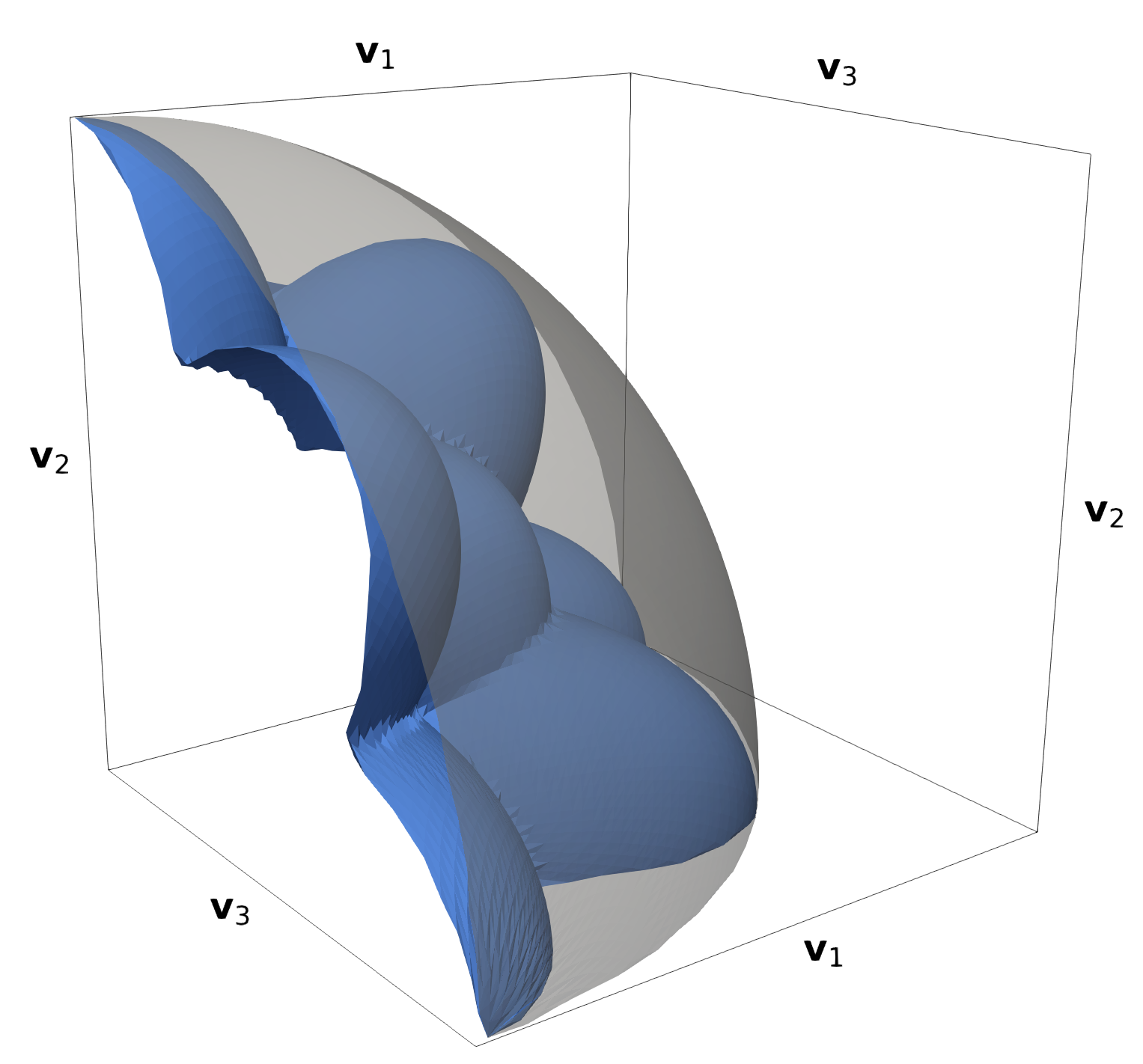
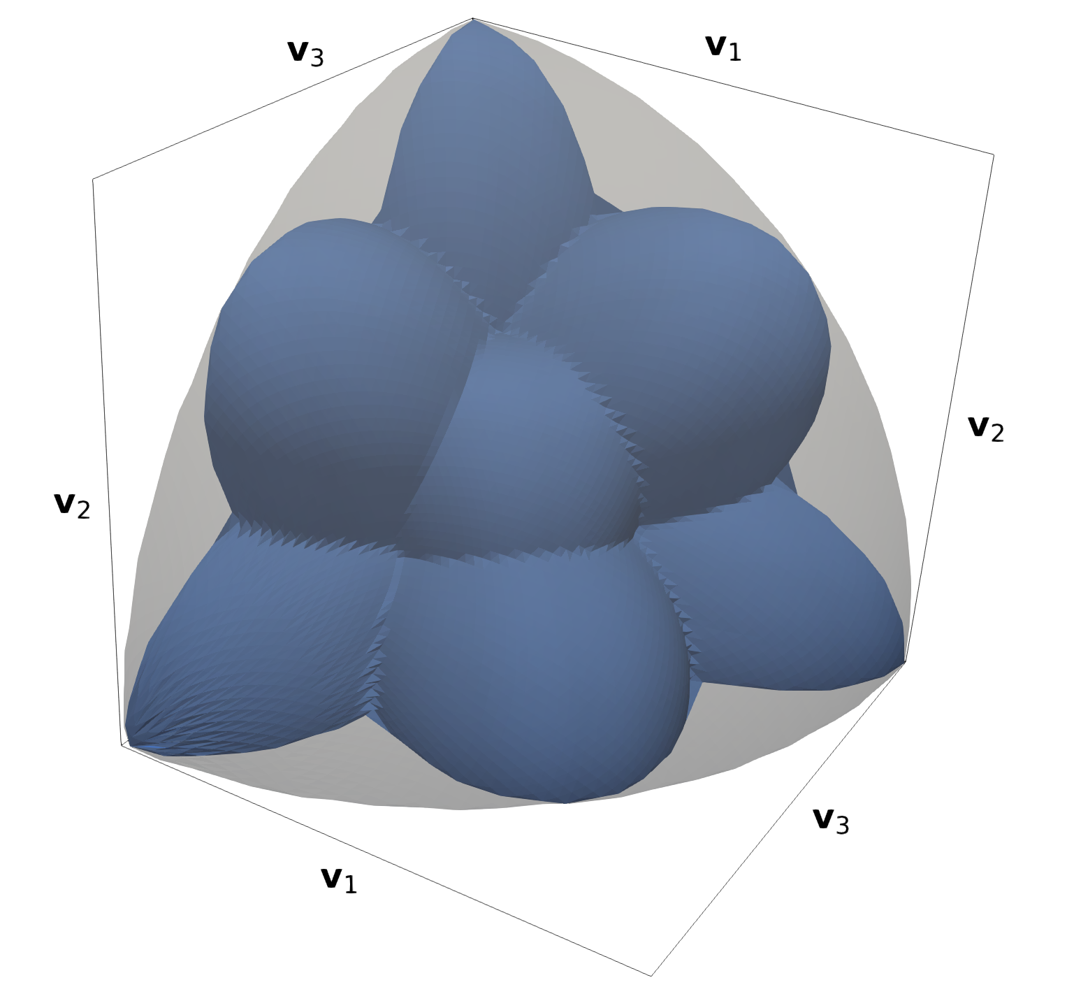
Figure 1: Two views on identical surfaces of polar plots of the maximum objective function value, i.e., $\mathbf{n}^{\otimes 4}(\varphi,\theta=0)::\mathds{A}$, of problem (3.50) for values $\lambda_{1}=1/3$ and $\lambda_{2}=1/3$. Results for the unconstrained triclinic case, i.e., $\mathcal{S}^{\text{problem}}=\mathcal{S}^{\text{triclinic}}$ are given in light gray, whereas results with restriction to the orthotropic subspace, i.e., $\mathcal{S}^{\text{problem}}=\mathcal{S}^{\text{orthotropic}}$ are shown in blue.

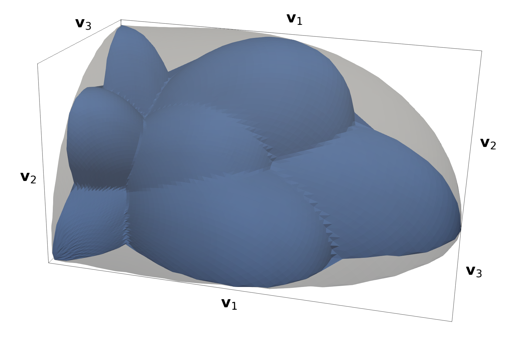
Figure 2: Polar plots of the maximum objective function value, i.e., $\mathbf{n}^{\otimes 4}(\varphi,\theta=0)::\mathds{A}$, of problem (3.50) for values $\lambda_{1}=1/2$ and $\lambda_{2}=1/4$. Results for the unconstrained triclinic case, i.e., $\mathcal{S}^{\text{problem}}=\mathcal{S}^{\text{triclinic}}$ are given in light gray, whereas results with restriction to the orthotropic subspace, i.e., $\mathcal{S}^{\text{problem}}=\mathcal{S}^{\text{orthotropic}}$ are shown in blue.

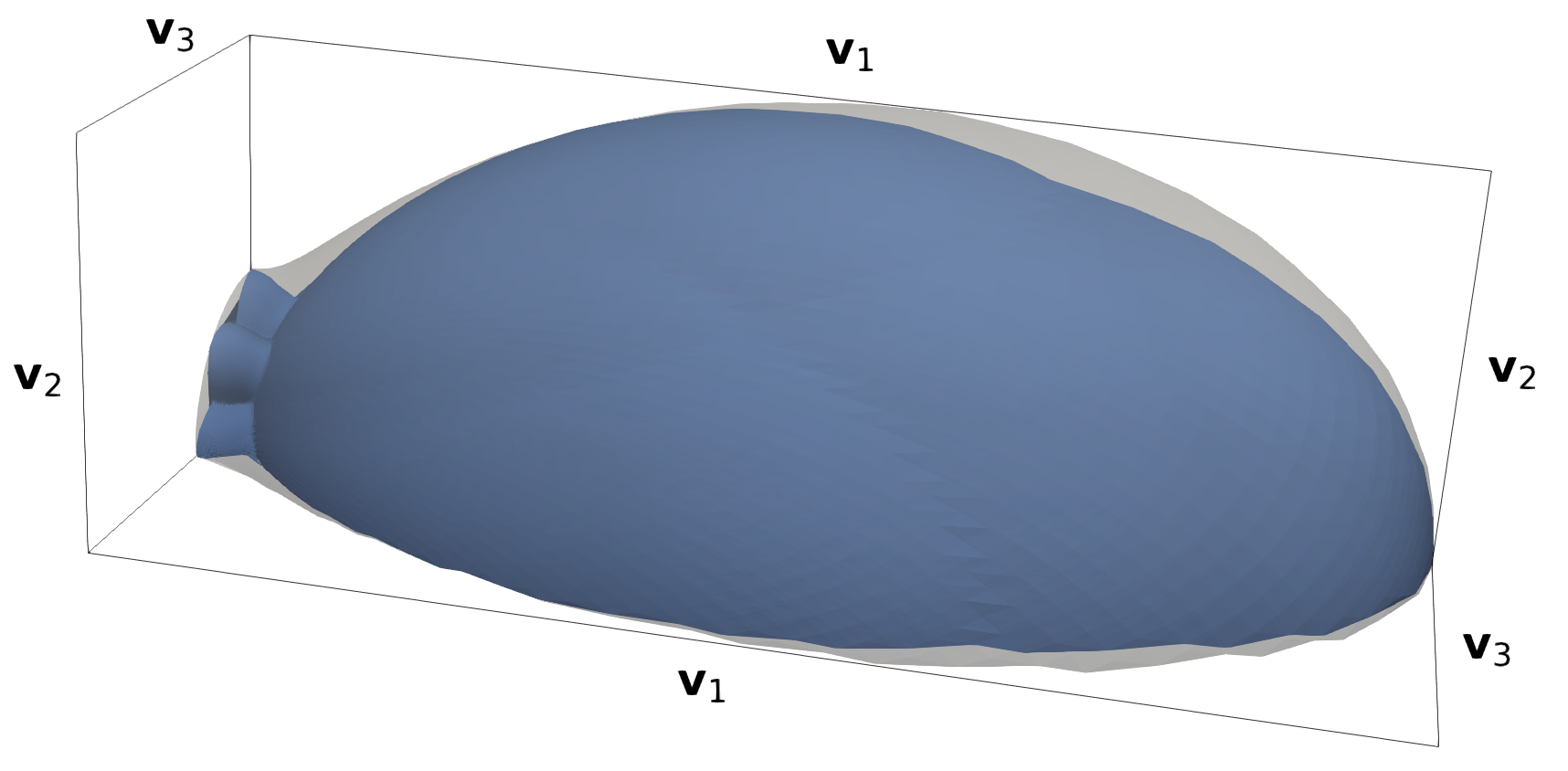
Figure 3: Polar plots of the maximum objective function value, i.e., $\mathbf{n}^{\otimes 4}(\varphi,\theta=0)::\mathds{A}$, of problem (3.50) for values $\lambda_{1}=8/10$ and $\lambda_{2}=1/10$. Results for the unconstrained triclinic case, i.e., $\mathcal{S}^{\text{problem}}=\mathcal{S}^{\text{triclinic}}$ are given in light gray, whereas results with restriction to the orthotropic subspace, i.e., $\mathcal{S}^{\text{problem}}=\mathcal{S}^{\text{orthotropic}}$ are shown in blue.

For the convenience of the reader, we translated typical constraints of problem (3.50) in terms of expressions $\mathds{G}_{k}::\mathds{A}=g_{k}$ with $k=1,...,m$ with tensors $\mathds{G}_{k}=G^{k}_{\xi\zeta}\,\mathbf{B}^{\mathbf{v}}_{\xi}\otimes\mathbf{B}^{\mathbf{v}}_{\zeta}$, see Table 1 in appendix B.

3.4 Results in three spatial dimensions

On a regular grid of points on one-eighth of the unit sphere, the maximum values of the objective function of problem (3.50) are visualized in Figures 1 to 3 as spherical plots. Due to the symmetry of the objective function specified by the quartic product $\mathbf{n}^{\otimes 4}$, inspecting the results on a grid of direction within one-eighth of the unit sphere is sufficient. Figures 1 to 3 differ by the given second-order fiber-orientation information, i.e., tuples $\mathbf{A}(\lambda_{1},\lambda_{2})$. Each of the figures contains two surfaces. The first surface plotted in light gray represents the maximum objective function obtained without material constraints on $\mathds{A}$, whereas the second surface plotted in blue represents the same quantity with $\mathds{A}$ restricted to orthotropic fourth-order fiber-orientation tensors, i.e., $\mathcal{S}^{\text{problem}}=\mathcal{S}^{\text{orthotropic}}$ in problem (3.50). Figures 1 to 3 demonstrate that restricting to the orthotropic subspace limits the possibility to obtain large values of the objective function in specific directions. Only in directions aligned with the axes of the eigensystem $\bigl{\{}\mathbf{v}_{i}\bigr{\}}$ as well as in directions with $(\varphi,\,\theta)\in\bigl{[}(0,\,45^{\circ}),\,(90^{\circ},\,45^{\circ}),\,(45^{\circ},\,0)\bigr{]}$, the constraint of orthotropy does not induce a restriction on the extreme value of the objective function. With increasing anisotropy of the specified second-order information, the consequences of the constraint onto the orthotropic subspace decrease.

3.5 Results in two spatial dimensions

If the given second-order fiber-orientation $\mathbf{A}$ is planar, i.e., fulfills the conditions $\lambda_{2}=1-\lambda_{1}$ and $1/2\leq\lambda_{1}\leq 1$, the constraint $\mathds{A}:\operatorname{\textrm{Id}}=\mathbf{A}(\lambda_{1},\,\lambda_{2})$ in problem (3.50) will enforce planarity of the resulting fourth-order fiber-orientation tensor $\mathds{A}$. Within the plane spanned by the directions $\mathbf{v}_{1}$ and $\mathbf{v}_{2}$, the maximum values of the objective function $\mathbf{n}^{\otimes 4}::\mathds{A}$ are plotted in Figures 10 to 10 with and without constraints in terms of material symmetry. The directions $\mathbf{n}(\varphi,\theta)$ within the plane $\mathbf{v}_{1}$ and $\mathbf{v}_{2}$ are characterized by the condition $\theta=0$ and varying angle $\varphi$. The values of the objective function obtainable for directions aligned with $\mathbf{v}_{1}$ and $\mathbf{v}_{2}$ are $\lambda_{1}$ and $\lambda_{2}$, respectively. For directions specified by angles $\theta\in\{0,\,45^{\circ},\,90^{\circ}\}$, the objective values obtained with or without material symmetry constraints are identical. For all other directions, restricting to the class of orthotropic fiber-orientation tensors $\mathds{A}$ limits the values of the objective function that can be attained. This limitation decreases as second-order fiber-orientation tensor information advances towards the uni-directional state, i.e., $\lambda_{1}\rightarrow 1$.

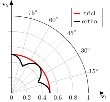
Figure 4: $\lambda_{1}=5/10$

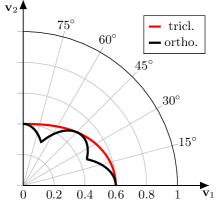
Figure 5: $\lambda_{1}=6/10$

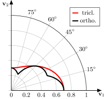
Figure 6: $\lambda_{1}=7/10$

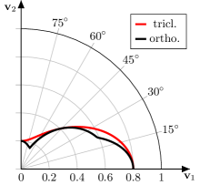
Figure 7: $\lambda_{1}=8/10$

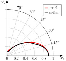
Figure 8: $\lambda_{1}=9/10$

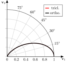
Figure 9: $\lambda_{1}=1$

Figure 10: Polar plots of the maximum objective function value, i.e., $\mathbf{n}^{\otimes 4}(\varphi,\theta=0)::\mathds{A}$, of problem (3.50) and $\lambda_{2}=1-\lambda_{1}$ for selected values of $\lambda_{1}$. Results are given for restriction to the triclinic or orthotropic subspace, i.e., $\mathcal{S}^{\text{problem}}=\mathcal{S}^{\text{triclinic}}$ or $\mathcal{S}^{\text{problem}}=\mathcal{S}^{\text{orthotropic}}$ respectively.

4 Conclusion

The work at hand showed that the set of candidates for fourth-order fiber-orientation tensors

$$\texttt{Cand}(d)=\left\{\mathds{A}\in\textrm{Sym}_{4}(d)\,\middle|\,S:\mathds{A}:S\geq 0\quad\text{for all}\quad S\in\textrm{Sym}_{2}(d),\quad\operatorname{\textrm{Id}}:\mathds{A}:\operatorname{\textrm{Id}}=1\right\}$$

represents all realizable fourth-order fiber-orientation tensors for the practically relevant spatial dimensions $d=2$ or $d=3$. This result provides an a-posteriori justification for the approach of Bauer and Böhlke [41] to characterize the variety of fourth-order fiber-orientation tensors based on tensor decompositions.
Our result has a number of interesting implications and applications. For a start, it permits assessing the realizability of a given fourth-order tensor as a fiber-orientation tensor in a simple and straightforward way. Consider, for instance, fiber-microstructure generators  [18, 19, 73], which serve as the basis for full-field simulations and where the fourth-order fiber-orientation tensor serves as the input. Then, if the prescribed tensor does not belong to the set $\texttt{Cand}(d)$, it cannot be realized by a fiber microstructure at all, independent of the size of the microstructure and the number of considered fibers. This simple fact provides constraints on fiber-orientation closure approximations used in fiber-orientation dynamics [37, 38], and may be used to re-evaluate their physical plausibility.
A second consequence concerns the effective elastic properties of short-fiber reinforced composites. It is well-known that, together with the volume fraction and the aspect ratio, the fourth-order fiber-orientation tensor is responsible for the effective elastic properties of such a composite [8, 9, 40]. Classical closure approximations, expressing the fourth-order fiber-orientation tensor as an isotropic tensor function of the second-order fiber-orientation tensor, are restricted, by definition, to orthotropic symmetry. In particular, the set of realizable effective stiffnesses is restricted to being orthotropic. Our computational investigations revealed that this restriction to orthotropy actually underestimates the achievable effective stiffnesses in particular directions for a prescribed second-order fiber-orientation tensor significantly. Thus, we expect that using the full phase space of fourth-order fiber-orientation tensors will be critical for exploiting the full lightweight potential of such short-fiber composites, e.g., by reducing safety factors. First steps in this direction were already proposed [3, 74, 75], and these works may be revisited with fresh impetus.
Last but not least let us stress the simplicity and utility of the connection between optimization of fiber microstructures described by fourth-order fiber-orientation tensors and semi-definite programming introduced in the work at hand. In particular due to the power of the available optimization solvers, new directions were opened to engineers working on fiber-reinforced components and their optimal design.

Declarations

Funding

JKB received funding by German Research Foundation (DFG, Deutsche Forschungsgemeinschaft) within the International Research Training Group “Integrated engineering of continuous-discontinuous long fiber reinforced polymer structures” (GRK 2078/2) - project 255730231. MS received partial support by the European Research Council within the Horizon Europe program - project 101040238.

Competing interests

The authors have no competing interests to declare that are relevant to the content of this article.

Appendix A Representing a fiber-orientation tensor as a non-negative sum of monomials

The purpose of this appendix is to show the monomial decomposition (2.9), i.e., that every fixed fiber-orientation tensor $A^{(k)}$ of even order may be written as a finite sum

$$A^{(k)}=\sum_{i=1}^{r}w_{i}\,q_{i}^{\otimes k}$$ (A.1)

with appropriate non-negative weights $w_{i}$, directions $q_{i}\in S^{d-1}$ and a non-negative integer $r$ not exceeding ${{k+d-1}\choose{d-1}}$, the dimension of the space of completely symmetric $k$-tensors in $d$ dimensions.
As a prerequisite, we require Carathéodory’s theorem [64], which states that any vector $z$ in an $m$-dimensional vector space $V$ which is represented in the form

$$z=\sum_{i=1}^{r}x_{i},\quad x_{i}\in V,$$ (A.2)

may also be written in the form

$$z=\sum_{i\in\mathcal{I}}\rho_{i}\,x_{i}$$ (A.3)

for an index set $\mathcal{I}\subseteq\{1,\ldots,r\}$ with at most $m$ elements and non-negative coefficients $\rho_{i}$. For the convenience of the reader, we include a short derivation, following Reznick [76]. Let us consider the case

$$z=\sum_{i=1}^{m+1}x_{i},\quad\text{i.e.},\quad r=m+1.$$ (A.4)

The vectors $\{x_{i}\}$ are linearly dependent, i.e., there are coefficients $c_{i}$, not all zero, s.t. the representation

$$0=\sum_{i=1}^{m+1}c_{i}\,x_{i}$$ (A.5)

holds. We may assume that some of the $c_{i}$ are positive. Indeed, if they were non-positive, we may multiply the coefficients by $-1$. Furthermore, suppose that the coefficients $c_{i}$ are ordered, upon possibly reindexing the sequence. In particular, the inequality

$$c_{i}\leq c_{m+1},\quad\text{i.e.},\quad 0\leq 1-\frac{c_{i}}{c_{m+1}},$$ (A.6)

holds for all $i=1,\ldots,m$ as $c_{m+1}>0$. We may rearrange equation (A.5) into the form

$$x_{m+1}=-\sum_{i=1}^{m}\frac{c_{i}}{c_{m+1}}\,x_{i}.$$ (A.7)

Inserting this representation into the expression (A.4) yields

$$z=\sum_{i=1}^{m}x_{i}+x_{m+1}=\sum_{i=1}^{m}\left(1-\frac{c_{i}}{c_{m+1}}\right)\,x_{i}.$$ (A.8)

Thus, we arrived at the conclusion of Carathéodory’s theorem for the special case (A.4) in view of the non-negativity assertion (A.6) of the coefficients.
The general case (A.2) with more terms $r>m+1$ follows from applying the special case (A.4) inductively.
Suppose a fiber-orientation tensor $A^{(k)}$ is given, i.e., there is some probability measure $\mu$ and a representation (2.4)

$$A^{(k)}=\int_{S^{d-1}}p^{\otimes k}\,d\mu(p).$$ (A.9)

The space of Radon measures may be considered as the continuous dual space of the space of continuous functions on the unit sphere $S^{d-1}$. It is a classical result of functional analysis (e.g., as a direct consequence of the Krein-Milman theorem [77, Example 8.16] ) that the sum of Dirac measures is dense in the space of Radon measures w.r.t. the weak-$*$ topology, i.e., there are $r_{j}$ positive weights $w_{i,j}$ and directions $p_{i,j}\in S^{d-1}$, s.t., for any continuous function $\phi:S^{d-1}\rightarrow\mathds{R}$, we have

$$\sum_{i=1}^{r_{j}}w_{i,j}\,\phi(p_{i,j})\rightarrow\int_{S^{d-1}}\phi(p)\,d\mu(p)\quad\text{as}\quad j\rightarrow\infty.$$ (A.10)

Choosing the monomials of homogeneity four as special continuous functions, we thus obtain the result

$$\sum_{i=1}^{r_{j}}w_{i,j}\,p_{i,j}^{\otimes k}\rightarrow A^{(k)}\quad\text{as}\quad j\rightarrow\infty.$$ (A.11)

By Carathéodory’s theorem (A.3) we can assume a uniform bound on the ranks $r_{j}$, i.e., it holds

$$\sum_{i=1}^{r}w_{i,j}\,p_{i,j}^{\otimes k}\rightarrow A^{(k)}\quad\text{as}\quad j\rightarrow\infty.$$ (A.12)

Appendix B Constraints

Typical constraints of problem (3.50) are translated in terms of the condition $\mathds{G}_{k}::\mathds{A}=g_{k}$ with $k=1,...,m$ with $\mathds{G}_{k}=G^{k}_{\xi\zeta}\,\mathbf{B}^{\mathbf{v}}_{\xi}\otimes\mathbf{B}^{\mathbf{v}}_{\zeta}$ in Table 1.

Description	Non-vanishing coefficients $G^{k}_{\xi\zeta}$	$g_{k}$
Complete symmetry of $\mathds{A}$	$G_{44}=1,\,G_{23}=-2$	0
	$G_{55}=1,\,G_{13}=-2$	0
	$G_{66}=1,\,G_{12}=-2$	0
	$G_{45}=1,\,G_{36}=-\sqrt{2}$	0
	$G_{46}=1,\,G_{25}=-\sqrt{2}$	0
	$G_{56}=1,\,G_{14}=-\sqrt{2}$	0
$\mathds{A}$ in eigensystem of $\mathbf{A}$	$G_{14}=G_{24}=G_{34}=1$	0
	$G_{15}=G_{25}=G_{35}=1$	0
	$G_{16}=G_{26}=G_{36}=1$	0
Normalization	$G_{11}=G_{22}=G_{33}=G_{44}=G_{55}=G_{66}=1$	1
Eigenvalues of $\mathds{A}:\operatorname{\textrm{Id}}$	$G_{11}=G_{12}=G_{13}=1$	$\lambda_{1}$
	$G_{12}=G_{22}=G_{23}=1$	$\lambda_{2}$
$\mathcal{S}^{\text{problem}}=\mathcal{S}^{\text{orthotropic}}$	$G_{24}=1$	0
	$G_{34}=1$	0
	$G_{15}=1$	0
	$G_{35}=1$	0
	$G_{16}=1$	0
	$G_{26}=1$	0

Table 1: Constraints of problem (3.50) reformulated in terms of the condition $\mathds{G}_{k}::\mathds{A}=g_{k}$ with $\mathds{G}_{k}=G^{k}_{\xi\zeta}\,\mathbf{B}^{\mathbf{v}}_{\xi}\otimes\mathbf{B}^{\mathbf{v}}_{\zeta}$

References

- [1] C. L. Tucker III, Fundamentals of Fiber Orientation: Description, Measurement and Prediction. Carl Hanser Verlag, 2022.
- [2] K. Kanatani, “Distribution of directional data and fabric tensors,” International Journal of Engineering Science, vol. 22, pp. 149–164, 1984.
- [3] S. G. Advani and C. L. Tucker, “The Use of Tensors to Describe and Predict Fiber Orientation in Short Fiber Composites,” Journal of Rheology, vol. 31, pp. 751–784, 1987.
- [4] T. Böhlke, F. Henning, A. Hrymak, L. Kärger, K. Weidenmann, and J. T. Wood, Continuous–Discontinuous Fiber-Reinforced Polymers: An Integrated Engineering Approach. Carl Hanser Verlag, 2019.
- [5] J. Görthofer, N. Meyer, T. D. Pallicity, L. Schöttl, A. Trauth, M. Schemmann, M. Hohberg, P. Pinter, P. Elsner, F. Henning, A. Hrymak, T. Seelig, K. Weidenmann, L. Kärger, and T. Böhlke, “Virtual process chain of sheet molding compound: Development, validation and perspectives,” Composites Part B: Engineering, vol. 169, pp. 133–147, 2019.
- [6] N. Meyer, S. Gajek, J. Görthofer, A. Hrymak, L. Kärger, F. Henning, M. Schneider, and T. Böhlke, “A probabilistic virtual process chain to quantify process-induced uncertainties in Sheet Molding Compounds,” Composites Part B: Engineering, p. 110380, 2022.
- [7] P. Zysset and A. Curnier, “An alternative model for anisotropic elasticity based on fabric tensors,” Mechanics of Materials, vol. 21, no. 4, pp. 243–250, 1995.
- [8] D. Jack and D. Smith, “The effect of fibre orientation closure approximations on mechanical property predictions,” Composites Part A: Applied Science and Manufacturing, vol. 38, no. 3, pp. 975–982, 2007.
- [9] D. A. Jack and D. E. Smith, “Elastic properties of short-fiber polymer composites, derivation and demonstration of analytical forms for expectation and variance from orientation tensors,” Journal of Composite Materials, vol. 42, no. 3, pp. 277–308, 2008.
- [10] N. Goldberg, F. Ospald, and M. Schneider, “A fiber orientation-adapted integration scheme for computing the hyperelastic Tucker average for short fiber reinforced composites,” Computational Mechanics, vol. 60, no. 4, pp. 595–611, 2017.
- [11] J. Köbler, M. Schneider, F. Ospald, H. Andrä, and R. Müller, “Fiber orientation interpolation for the multiscale analysis of short fiber reinforced composite parts,” Computational Mechanics, vol. 61, no. 6, pp. 729–750, 2018.
- [12] P. A. Hessman, F. Welschinger, K. Hornberger, and T. Böhlke, “On mean field homogenization schemes for short fiber reinforced composites: unified formulation, application and benchmark,” International Journal of Solids and Structures, p. 111141, 2021.
- [13] J. Feder, “Random sequential adsorption,” Journal of Theoretical Biology, vol. 87, no. 2, pp. 237–254, 1980.
- [14] Y. Pan, L. Iorga, and A. A. Pelegri, “Numerical generation of a random chopped fiber composite RVE and its elastic properties,” Composites Science and Technology, vol. 68, no. 13, pp. 2792–2798, 2008.
- [15] H. Altendorf and D. Jeulin, “Random-walk-based stochastic modeling of three-dimensional fiber systems,” Physical Review E, vol. 83, no. 4, p. 041804, 2011.
- [16] V. Salnikov, D. Choï, and P. Karamian-Surville, “On efficient and reliable stochastic generation of RVEs for analysis of composites within the framework of homogenization,” Computational Mechanics, vol. 55, no. 1, pp. 127–144, 2015.
- [17] W. Tian, L. Qi, J. Zhou, J. Liang, and Y. Ma, “Representative volume element for composites reinforced by spatially randomly distributed discontinuous fibers and its applications,” Composite Structures, vol. 131, pp. 366–373, 2015.
- [18] M. Schneider, “The sequential addition and migration method to generate representative volume elements for the homogenization of short fiber reinforced plastics,” Computational Mechanics, vol. 59, no. 2, pp. 247–263, 2017.
- [19] A. Mehta and M. Schneider, “A sequential addition and migration method for generating microstructures of short fibers with prescribed length distribution,” Computational Mechanics, vol. 70, no. 4, pp. 829–851, 2022.
- [20] G. B. Jeffery, “The motion of ellipsoidal particles immersed in a viscous fluid,” Proceedings of the Royal Society of London. Series A, Containing papers of a mathematical and physical character, vol. 102, no. 715, pp. 161–179, 1922.
- [21] F. Folgar and C. L. Tucker III, “Orientation behavior of fibers in concentrated suspensions,” Journal of reinforced plastics and composites, vol. 3, no. 2, pp. 98–119, 1984.
- [22] S. G. Advani and C. L. Tucker III, “A numerical simulation of short fiber orientation in compression molding,” Polymer composites, vol. 11, no. 3, pp. 164–173, 1990.
- [23] S. Yamamoto and T. Matsuoka, “A method for dynamic simulation of rigid and flexible fibers in a flow field,” The Journal of Chemical Physics, vol. 98, no. 1, pp. 644–650, 1993.
- [24] J. Wang, J. F. O’Gara, and C. L. Tucker III, “An objective model for slow orientation kinetics in concentrated fiber suspensions: Theory and rheological evidence,” Journal of Rheology, vol. 52, no. 5, pp. 1179–1200, 2008.
- [25] J. H. Phelps and C. L. Tucker III, “An anisotropic rotary diffusion model for fiber orientation in short-and long-fiber thermoplastics,” Journal of Non-Newtonian Fluid Mechanics, vol. 156, no. 3, pp. 165–176, 2009.
- [26] R. S. Bay and C. L. Tucker III, “Stereological measurement and error estimates for three-dimensional fiber orientation,” Polymer Engineering & Science, vol. 32, no. 4, pp. 240–253, 1992.
- [27] A. Clarke, G. Archenhold, and N. Davidson, “A novel technique for determining the 3D spatial distribution of glass fibres in polymer composites,” Composites science and technology, vol. 55, no. 1, pp. 75–91, 1995.
- [28] J.-M. Geusebroek, A. W. Smeulders, and J. Van De Weijer, “Fast anisotropic Gauss filtering,” IEEE transactions on image processing, vol. 12, no. 8, pp. 938–943, 2003.
- [29] S. C. Cowin, “The relationship between the elasticity tensor and the fabric tensor,” Mechanics of materials, vol. 4, no. 2, pp. 137–147, 1985.
- [30] D. Le Bihan, J.-F. Mangin, C. Poupon, C. A. Clark, S. Pappata, N. Molko, and H. Chabriat, “Diffusion tensor imaging: concepts and applications,” Journal of Magnetic Resonance Imaging: An Official Journal of the International Society for Magnetic Resonance in Medicine, vol. 13, no. 4, pp. 534–546, 2001.
- [31] S. Mori and P. C. Van Zijl, “Fiber tracking: principles and strategies–a technical review,” NMR in Biomedicine: An International Journal Devoted to the Development and Application of Magnetic Resonance In Vivo, vol. 15, no. 7-8, pp. 468–480, 2002.
- [32] P. J. Basser and D. K. Jones, “Diffusion-tensor MRI: theory, experimental design and data analysis–a technical review,” NMR in Biomedicine: An International Journal Devoted to the Development and Application of Magnetic Resonance In Vivo, vol. 15, no. 7-8, pp. 456–467, 2002.
- [33] D. Taylor and M. Bushell, “The spatial mapping of translational diffusion coefficients by the NMR imaging technique,” Physics in medicine & biology, vol. 30, no. 4, p. 345, 1985.
- [34] D. Le Bihan, E. Breton, D. Lallemand, P. Grenier, E. Cabanis, and M. Laval-Jeantet, “MR imaging of intravoxel incoherent motions: application to diffusion and perfusion in neurologic disorders,” Radiology, vol. 161, no. 2, pp. 401–407, 1986.
- [35] P. W. Schaefer, P. E. Grant, and R. G. Gonzalez, “Diffusion-weighted MR imaging of the brain,” Radiology, vol. 217, no. 2, pp. 331–345, 2000.
- [36] S. Nomura, H. Kawai, I. Kimura, and M. Kagiyama, “General description of orientation factors in terms of expansion of orientation distribution function in a series of spherical harmonics,” Journal of Polymer Science Part A-2: Polymer Physics, vol. 8, no. 3, pp. 383–400, 1970.
- [37] J. S. Cintra Jr and C. L. Tucker III, “Orthotropic closure approximations for flow-induced fiber orientation,” Journal of Rheology, vol. 39, no. 6, pp. 1095–1122, 1995.
- [38] D. H. Chung and T. H. Kwon, “Improved model of orthotropic closure approximation for flow induced fiber orientation,” Polymer Composites, vol. 22, no. 5, pp. 636–649, 2001.
- [39] J. Linn, “The Folgar-Tucker model as a differential algebraic system for fiber orientation calculation,” Berichte des Fraunhofer-Instituts für Techno- und Wirtschaftsmathematik (ITWM Report), no. 75, 2005.
- [40] V. Müller and T. Böhlke, “Prediction of effective elastic properties of fiber reinforced composites using fiber orientation tensors,” Composites Science and Technology, vol. 130, pp. 36–45, 2016.
- [41] J. K. Bauer and T. Böhlke, “Variety of fiber orientation tensors,” Mathematics and Mechanics of Solids, vol. 27, no. 7, pp. 1185–1211, 2022.
- [42] M. Moakher, “The algebra of fourth-order tensors with application to diffusion MRI,” in Visualization and Processing of Tensor Fields, pp. 57–80, Springer, 2009.
- [43] J. Rahmoun, D. Kondo, and O. Millet, “A 3D fourth order fabric tensor approach of anisotropy in granular media,” Computational Materials Science, vol. 46, no. 4, pp. 869–880, 2009.
- [44] Y. T. Weldeselassie, A. Barmpoutis, and M. S. Atkins, “Symmetric positive semi-definite Cartesian tensor fiber orientation distributions (CT-FOD),” Medical Image Analysis, vol. 16, no. 6, pp. 1121–1129, 2012.
- [45] A. Ghosh, T. Papadopoulo, and R. Deriche, “Biomarkers for HARDI: 2nd & 4th order tensor invariants,” in 2012 9th IEEE International Symposium on Biomedical Imaging (ISBI), pp. 26–29, IEEE, 2012.
- [46] R. Moreno, Ö. Smedby, and D. H. Pahr, “Prediction of apparent trabecular bone stiffness through fourth-order fabric tensors,” Biomechanics and modeling in Mechanobiology, vol. 15, no. 4, pp. 831–844, 2016.
- [47] A. Spencer, “A note on the decomposition of tensors into traceless symmetric tensors,” International Journal of Engineering Science, vol. 8, no. 6, pp. 475–481, 1970.
- [48] S. Forte and M. Vianello, “Symmetry classes for elasticity tensors,” Journal of Elasticity, vol. 43, no. 2, pp. 81–108, 1996.
- [49] J. Jerphagnon, D. Chemla, and R. Bonneville, “The description of the physical properties of condensed matter using irreducible tensors,” Advances in Physics, vol. 27, no. 4, pp. 609–650, 1978.
- [50] B. Adams, J. Boehler, M. Guidi, and E. Onat, “Group theory and representation of microstructure and mechanical behavior of polycrystals,” Journal of the Mechanics and Physics of Solids, vol. 40, no. 4, pp. 723–737, 1992.
- [51] S. C. Cowin, “Properties of the anisotropic elasticity tensor,” The Quarterly Journal of Mechanics and Applied Mathematics, vol. 42, no. 2, pp. 249–266, 1989.
- [52] J. Rychlewski, “A qualitative approach to Hooke’s tensors. Part I,” Archives of Mechanics, vol. 52, no. 4-5, pp. 737–759, 2000.
- [53] J. K. Bauer, Fiber orientation tensors and mean field homogenization: Application to sheet molding compound. PhD thesis, in process.
- [54] J. K. Bauer and T. Böhlke, “Fiber orientation distributions based on planar fiber orientation tensors of fourth order,” Mathematics and Mechanics of Solids, p. 10812865221093958, 2022.
- [55] J. K. Bauer and T. Böhlke, “On the dependence of orientation averaging mean field homogenization on planar fourth-order fiber orientation tensors,” Mechanics of Materials, vol. 170, p. 104307, 2022.
- [56] F. Folgar and C. L. Tucker III, “Orientation behaviour of fibers in concentrated suspensions,” Journal of Reinforced Plastics and Composites, vol. 3, pp. 98–119, 1984.
- [57] K.-H. Han and Y.-T. Im, “Modified hybrid closure approximation for prediction of flow-induced fiber orientation,” Journal of Rheology, vol. 43, no. 3, pp. 569–589, 1999.
- [58] D. H. Chung and T. H. Kwon, “Invariant-based optimal fitting closure approximation for the numerical prediction of flow-induced fiber orientation,” Journal of Rheology, vol. 46, no. 1, pp. 169–194, 2002.
- [59] S. Montgomery-Smith, W. He, D. A. Jack, and D. E. Smith, “Exact tensor closures for the three-dimensional Jeffery’s equation,” Journal of Fluid Mechanics, vol. 680, pp. 321–335, 2011.
- [60] S. Montgomery-Smith, D. Jack, and D. E. Smith, “The fast exact closure for Jeffery’s equation with diffusion,” Journal of Non-Newtonian Fluid Mechanics, vol. 166, no. 7-8, pp. 343–353, 2011.
- [61] T. Karl, D. Gatti, B. Frohnapfel, and T. Böhlke, “Asymptotic fiber orientation states of the quadratically closed Folgar–Tucker equation and a subsequent closure improvement,” Journal of Rheology, vol. 65, no. 5, pp. 999–1022, 2021.
- [62] C. L. Tucker III, “Planar fiber orientation: Jeffery, non-orthotropic closures, and reconstructing distribution functions,” Journal of Non-Newtonian Fluid Mechanics, p. 104939, 2022.
- [63] D. Hilbert, “Über die Darstellung definiter Formen als Summe von Formenquadraten,” Mathematische Annalen, vol. 32, no. 3, pp. 342–350, 1888.
- [64] C. Carathéodory, “Über den Variabilitätsbereich der Fourier’schen Konstanten von positiven harmonischen Funktionen,” Rendiconti del Circolo Matematico di Palermo, vol. 32, no. 1, pp. 193–217, 1911.
- [65] P. Comon, G. Golub, L.-H. Lim, and B. Mourrain, “Symmetric Tensors and Symmetric Tensor Rank,” SIAM Journal on Matrix Analysis and Applications, vol. 30, no. 3, pp. 1254–1279, 2008.
- [66] W. Thomson, “Elements of a mathematical theory of elasticity,” Philosophical Transactions of the Royal Society of London, no. 146, pp. 481–498, 1856.
- [67] J. Mandel, “Généralisation de la théorie de plasticité de WT Koiter,” International Journal of Solids and Structures, vol. 1, pp. 273 – 295, 1965.
- [68] R. T. Rockafellar, Convex analysis. Princeton Landmarks in Mathematics and Physics, Princeton: Princeton University Press, 1996.
- [69] M. D. Choi, T. Y. Lam, and B. Reznick, “Even symmetric sextics,” Mathematische Zeitschrift, vol. 195, pp. 559–580, 1987.
- [70] B. Reznick, “Some concrete aspects of Hilbert’s 17th Problem,” Contemporary Mathematics, vol. 253, pp. 251–272, 2000.
- [71] G. Blekherman, “There are significantly more nonegative polynomials than sums of squares,” Israel Journal of Mathematics, vol. 153, pp. 355–380, 2006.
- [72] W. Voigt, Lehrbuch der Kristallphysik, vol. 34. BG Teubner, 1910.
- [73] M. Schneider, “An algorithm for generating microstructures of fiber-reinforced composites with long fibers,” International Journal for Numerical Methods in Engineering, vol. 123, no. 24, pp. 6197–6219, 2022.
- [74] M. C. Altan, S. Subbiah, S. I. Güçeri, and R. B. Pipes, “Numerical prediction of three-dimensional fiber orientation in Hele-Shaw flows,” Polymer Engineering & Science, vol. 30, pp. 848–859, 1990.
- [75] D. A. Jack, “Sixth-order Fitted Closures for Short-fiber Reinforced Polymer Composites,” Journal of Thermoplastic Composite Materials, vol. 19, no. 2, pp. 217–246, 2006.
- [76] B. Reznick, Sums of even powers of real linear forms. No. 96 in Memoirs of the American Mathematical Society, Boston: American Mathematical Society, 1992.
- [77] B. Simon, Extreme points and the Krein–Milman theorem, p. 120–135. Cambridge Tracts in Mathematics, Cambridge University Press, 2011.