Gauging the Gauge
and Anomaly Resolution

Abstract

In this paper, we explore the algebraic and geometric structures that arise from a procedure we dub "gauging the gauge", which involves the promotion of a certain global, coordinate independent symmetry to a local one. By gauging the global 1-form shift symmetry in a gauge theory, we demonstrate that the structure of a Lie algebra crossed-module and its associated 2-gauge theory arises. Moreover, performing this procedure once again on a 2-gauge theory generates a 3-gauge theory, based on Lie algebra 2-crossed-modules. As such, the physical procedure of "gauging the gauge" can be understood mathematically as a categorification. Applications of such higher-gauge structures are considered, including gravity, higher-energy physics and condensed matter theory. Of particular interest is the mechanism of anomaly resolution, in which one introduces a higher-gauge structure to absorb curvature excitations. This mechanism has been shown to allow one to consistently gauge an anomalous background symmetry in QFT .

0 Introduction

Understanding the symmetries of a physical system is tantamount to constructing a mathematical model that describes its properties. From condensed matter to higher-energy physics, models such as Ginzburg-Landau theory of phase transitions and the Standard Model, are based upon this fact. In fact, sometimes a handle on symmetry is all we have in more esoteric areas of theoretical physics, such as string theory and quantum gravity, as no sufficient experimental data and/or techniques are yet available.

In general, there are two notions of symmetry in a physical system: global and local. Global symmetries act uniformly upon the entire system, while the action of the local symmetry depends on the particular physical configuration in $X$. Of course, the latter is the more general notion, and a global symmetry can be made local by the procedure of gauging: we promote the constant group elements to depend on points in $X$. Because of the locality requirement for the symmetry, the notion of derivative is typically not transforming covariantly unless one adds some compensating term, a connection. In a sense, the notion of connection encodes the break down of the covariance of the transformation of the derivative.

The structure of physical systems with local symmetries is described geometrically by a principal bundle $P\rightarrow X$ [1]; solutions to the equations of motion determine configurations on $P$ that represent a class of physical configurations on $X$ under the action of transformations by $G$. Many local geometric quantities on $P$, such as connection and curvature, are important for understanding the physical system.

Moreover, recent developments in condensed matter theory [2, 3, 4] had also shown that, aside from symmetry, topology plays a central role in the characterization of physical systems as well. In particular, the topology of the principal bundle $P\rightarrow X$ determines the presence of defects in the physical system, which can alter its physical properties in a drastic, non-perturbative manner [5, 6]. Also from a quantum gravity point of view, understanding topology can be relevant. Indeed, one might need to sum over all the possible topological configurations to build the transition amplitudes. In fact, for example, 3d gravity is essentially about the topology of spacetime, since it does not have local degrees of freedom.

It is important to note that there are different notions of "topological features". We can characterize the topology of the manifold of interest (such as spacetime), the topology of the principal bundle in the case of a gauge theory, which is related to the cohomological features of the gauge symmetry. The notion of magnetic monopole is related to the topology and geometry of the principal bundle. Such topological features in the gauge symmetry structure appear for example in quantum field theory, where they manifest as obstructions to defining the path integral [4, 7]. Typically, all such non-trivial topological features can be cast as anomalies, as due to their presence, some quantities (such as $d_{A}F$, or the 1- or 2-curvature) are non-trivial.

Giving a physical system, one typically tries to identify the symmetries in order to characterize the physical conserved quantities or the quantum theory (built as representations of this symmetry). Conversely, one can construct new symmetry structures and then try to identify some physical systems associated to them. One way to proceed is to categorify the notion of symmetries. It consists in using category theory tools to build new types of symmetries [8]. For example the notion of 2-group comes up naturally when considering higher-dimensional homotopy types [9, 10]. This approach relies on beautiful elaborate mathematics which might leave the interested reader wondering what are the physical motivations behind it. One goal of this paper is to argue that this categorification process can be seen as a gauging principle so that dealing with categorified local symmetries here is nothing else than gauging (a gauge). Hence a $(n+1)$-gauge theory can be interpreted as a gauged $n$-gauge theory. This idea is not new to the expert in categorical symmetries, but we try to make this point in a pedagogical way, using mostly basic tools of gauge theory and exploring how and when there could be some generalizations.

Once we have in hand some new symmetries, one needs to identify systems where such symmetries are realized. It has been known since some times that categorified symmetries are the natural structure to probe the notion of topology, thanks to the categorical ladder [11, 12]. For example the moduli space of flat connection can be used to characterize topological features of a 3d manifold [13, 14]. One can expect the moduli space of flat 2-connections (ie. with a categorified gauge symmetry) to probe some topological features of a 4d manifold [15, 16, 17]. These categorified symmetries have been explored from the physics perspective, mainly in the context of condensed matter [18, 19, 20] or string theory [21, 22]. In this paper we would like to highlight the fact that a another physical application of these categorified symmetries is to reproduce some of the feature of the topological anomalies we discussed above, without any such singular structure. For example, it is well-known that a magnetic monopole corresponds to a singular structure in the principal bundle, namely the Bianchi identity is violated, due to the fact that $d^{2}\neq 0$. Recent work has pointed out that such magnetic monopole physics can be recovered using a 2-gauge theory, without a violation of the Bianchi identity [23, 24, 25]. We show that something similar exists one more level up: we can consider a violation of the 2-Bianchi identity and absorb it in a non-singular 3-gauge theory. This is one of our new results.

The article is organized as follows.

In section 1, we recall quickly what is the usual notion of gauging. Then in section 2, we proceed to gauge the gauge by making local, in some sense, a hidden shift symmetry for the 1-curvature. The lack of covariance is encoded in a 2-connection. To have a general structure, the notion of crossed module, equivalent to a strict 2-group, is naturally introduced. We then discuss the different possible generalizations of the gauge symmetry structure. In particular, we describe how the structures of a weak Lie 2-algebra [26, 8] manifests when the (1-)Bianchi identity is relaxed. We also point out how having a specific non-zero 2-curvature can be related to the topological properties of the crossed module, encoded by the so-called Postnikov class [18]. We discuss then how the gauge symmetry structure needs to be adapted to account for such case.

While the results are strictly not new in this section, we made an effort to have an original presentation using a language that would be accessible to a more physically minded reader.

In section 2.5, we discuss some applications of 2-gauge theory. The main example is a topological theory, 2-BF theory [27, 28], which can be seen in some sense as a sort of BF theory. According to the space-time dimension, there are different types of applications. For example, in 3D, BF theory (ie. in particular 3d gravity) can be seen as a specific (2-)gauge fixed 2-BF theory. This had not been pinpointed before, to the best of our knowledge, and it could provide some interesting new directions to explore 3d gravity. In 4D, 2-BF theory is somehow the canonical topological theory. Its symmetry structure is associated to a 2-Drinfeld double and one would expect that topological excitations (string like or point like) should be encoded in terms of representations of 2-Drinfeld double, a direct generalization of the Drinfeld double in the 3d case. In 5D, it was known that 2-gauge symmetries could be related to the $w_{2}$ and $w_{3}$ Stiefel-Whitney classes [29, 30]. We highlight how this can be done through a 2-BF theory, which was not emphasized previously to the best of our knowledge.

Finally, we also discuss how the magnetic monopole can be recovered from considering a 2-gauge theory, with some interesting mobility conditions on the currents [25]. This is illustrating the notion of anomaly resolution, that is we exchange a system with non-trivial topological feature (in this case the a non-trivial topology for the principal bundle) for a system with an extra gauge symmetry structure which allows to reproduce the physics of the non-trivial topological feature [23, 24]. A closely related notion of anomaly inflow [31], and its relation to higher symmetries [32], has also been studied recently in the high-energy physics literature.

In section 3, we gauge the 2-gauge, to obtain a 3-gauge theory. The gauging follows the same step as in the 2-gauge case. We introduce some more general shift transformation, which do not leave the derivative (of the 2-connection) covariant. The lack of covariance is encoded in a 3-connection. We highlight where some constraints, such as the 1-Bianchi identity, the Peiffer condition, can be weakened. We construct the 3-gauge transformations given in terms of a 2-crossed module. As a direct generalization of the crossed module case, we discuss how the presence of a non-trivial Postnikov class for the 2-crossed module is associated with a non-zero 3-curvature and non-trivial 1-gauge transformations.

In section 3.3, we discuss some applications when dealing with a 3-gauge theory. We recall some of the main features of a 3-BF theory, following [33]. We point out that we would expect to have a 3-Drinfeld double symmetry at play in this case (for a 5d spacetime). With the string Lie 2-algebra [34, 35] as an explicit example, we then study a categorified analogue of the results in [23, 24]: that an anomalous 2-group symmetry gauges into a non-anomalous mixed 0-, 1- and 2-form symmetry governed by a 3-group. Moreover, the subsequent 3-Yang-Mills theory $S_{\text{3YM}}$ and the associated 3-conservation laws yield new and interesting higher-mobility constraints that have not appeared previously, as far as we know.

The Appendices provide some mathematical background and results. In Appendix A, we describe in full detail the classification of strict Lie 2-algebras/Lie algebra crossed-modules by a degree-3 cohomology class [36], called the Postnikov class. In Appendix B, we explore what the Postnikov class says about our 2-gauge theories, and we also describe the relationship between the Postnikov class and a similar quantity, called the Jacobiator, in a weak Lie 2-algebra [34, 35].

1 Gauging the 0-gauge

In the following, we first review in a pedestrian way the notion of gauging a global symmetry. This is standard material, for which one can find many introductions (eg. [1]).

Let $X$ denote a $d$-dimensional smooth manifold admitting an action by a Lie group $G$. Consider a (smooth) function $\phi\in C^{\infty}(X)$ transforming under a representation $\pi:G\rightarrow\operatorname{GL}(V)$ of the group $G$ for some vector space $V$, that is $\phi\in C^{\infty}(X)\otimes V$, namely $\phi$ lies in the algebra of $V$-valued smooth functions on $X$.

Note that $\pi$ is an homomorphism, and the field $\phi$ transforms as

$$\phi(x)\rightarrow\pi(g)\phi(x),\qquad g\in G.$$

If $g\in G$ is not a $G$-valued function of $X$, then the derivative $d\phi$ transforms covariantly,

$$d\phi\rightarrow d(\pi(g)\phi)=\pi(g)d\phi,$$

and $G$ encodes a (global) 0-gauge symmetry.

We can promote $g$ to be a $G$-valued function of $X$ itself, such that we still have the transformation law

$$\phi(x)\rightarrow\pi({g(x)})\phi(x)\equiv g(x)\cdot\phi(x)=\phi^{\prime}.$$

In this case we are dealing with a principal bundle with fiber $G$ and base $X$.

The Leibniz rule for the exterior derivative $d$ dictates that

$$d\phi\rightarrow g(d+g^{-1}dg)\cdot\phi.$$

As such it is not $d\phi$ that transforms covariantly, but the covariant derivative $\nabla\phi\equiv(d+gdg^{-1})\phi$. Indeed, we can introduce the connection $A=gdg^{-1}\in\Omega^{1}(X)\otimes\mathfrak{g}$, to compensate for the lack of covariance,

$$gA\phi=d\phi^{\prime}-gd\phi\rightarrow A=g^{-1}dg.$$ (1.1)

Notice that this connection has a natural invariance symmetry under the left translation for all $h\in G$ constant (ie. $dh=0$).

$$(hg)^{-1}d(hg)=g^{-1}dg$$ (1.2)

This is the well-known fact that this is a left-invariant form.

Given the covariant derivative $\nabla=d+g^{-1}dg$, its associated curvature

$$\operatorname{cur}\nabla=[\nabla,\nabla]=d(g^{-1}dg)+(g^{-1}dg)\wedge(g^{-1}dg)=0$$

vanishes, where we have used the identity $d(1)=d(g^{-1}g)=(dg^{-1})g+g^{-1}dg=0$. This means that the connection $A=g^{-1}dg$ is flat.

The 0-form symmetry and 1-gauge transformations.

The connection 1-form in an arbitrary gauge, $A\in\Omega^{1}(X)\otimes\mathfrak{g}$ and the associated curvature 2-form $\operatorname{cur}A=F=d_{A}A=dA+\frac{1}{2}[A\wedge A]$ transform as

$$A\rightarrow A^{g}=g^{-1}Ag+g^{-1}dg,\qquad F\rightarrow F^{g}=g^{-1}Fg.$$ (1.3)

Expressing $g=\exp\lambda\approx 1+\lambda$ in terms of the infinitesimal gauge parameter $\lambda\in\Omega^{0}(X)\otimes\mathfrak{g}$, we achieve the (infinitesimal) (1-)gauge transformation laws

$$A \rightarrow A^{\lambda}=A+[A,\lambda]+d\lambda\equiv A+d_{A}\lambda,$$

$$F \rightarrow F^{\lambda}=F+[F,\lambda].$$

They endow the bundle $P\rightarrow X$ with a 0-form gauge symmetry parameterized by $\lambda$.

The Bianchi identity reads $d_{A}F=dF+[A\wedge F]=0$, which holds in general for any principal $G$-bundle with connection $A$. Since $F$ transforms covariantly, $d_{A}F$ also transforms covariantly

$$d_{A}F\rightarrow d_{A^{\lambda}}F^{\lambda}=d_{A}F+[d_{A}F,\lambda].$$

It is possible (and consistent) to achieve a 1-curvature anomaly $F=\sigma\neq 0$, as long as $\sigma\in\Omega^{2}(X)\otimes\mathfrak{g}$ satisfies $d_{A}\sigma=0$, and transforms covariantly $\sigma\rightarrow g^{-1}\sigma g$.

Global 1-form symmetry.

What we have recalled here is that, by gauging the global symmetry understood as a "0-gauge" symmetry, we obtain an ordinary 1-gauge bundle $P\rightarrow X$ that is flat. However, one may notice that the curvature 2-form $F=d_{A}A$ has a hidden symmetry in the presence of a non-trivial center $Z(\mathfrak{g})$. This symmetry is given by

$$A\rightarrow A+\alpha,$$ (1.4)

where $\alpha$ is a closed 1-form valued in the center $Z(\mathfrak{g})$ of the Lie algebra $\mathfrak{g}$, that is $\alpha\in\Omega^{1}_{0}(X)\otimes Z(\mathfrak{g})$. As such the above gauge structure in fact manifests a "1-form symmetry" parameterized by $\alpha$, on top of the pre-existing 1-gauge 0-form symmetry parameterized by $\lambda$. This 1-form symmetry is affecting the connection $A$ but not its curvature.

2 Gauging the 1-gauge

In the 1-gauge case, we have highlighted two different types of invariance, one specified by a left multiplication, in (1.2), the other one by a 1-form shift in (1.4). It is natural to ask what happens when we gauge each symmetry, ie. we make them non-constant. For the former, making $h$ non-constant amounts to just another gauge transformation, so there is nothing new to be gained. The latter is more interesting, as it leads to some new structures.

Relaxing the condition that $\alpha$ in (1.4) is constant and valued in the center $Z(\mathfrak{g})$ will be called "gauging the 1-form gauge". So we allow $\alpha\rightarrow a$ to become a generic 1-form $a\in\Omega^{1}(X)\otimes\mathfrak{g}$ that has non-trivial coordinate dependence on $X$, similar to the gauging procedure for the global/0-gauge symmetry.

2.1 Shifting the connection

Typically, one may a priori take a gauge bundle $P\rightarrow X$ with the non-trivial curvature $F=\sigma\neq 0$, then study the associated gauge theory. Alternatively, we may perform a particular 1-form shift such that $F\rightarrow F^{\prime}$ is transformed to a non-trivial value.

Indeed, under a generic 1-form shift.

$$A\rightarrow A^{\prime}=A+a,$$

we see that the curvature transforms accordingly as

$$F\rightarrow F^{\prime}=d_{A^{\prime}}A^{\prime}=F+d_{A}a+\frac{1}{2}[a\wedge a]=F+d_{A}a+\frac{1}{2}[a\wedge a].$$ (2.1)

In the gauge where $A=0$, we just have

$$F^{\prime}=da+\frac{1}{2}[a\wedge a],$$

which is the curvature of $a$ considered as a $G$-connection. As such we may shift the curvature to any value from zero, which serves as the central key fact for anomaly resolution discussed later. Usually, the "gauging" story ends here, and we deal with an arbitrary curvature associated to the connection in a particular 1-form gauge $A=a$.

However, the above also shows that, by considering the 1-form shift as a higher-form gauge symmetry, the (1-)curvature quantity $F$ is a gauge datum, the notion of curvature is gauge dependent. We have then a pair of gauge structures, one encoded in $g$ which in a sense encodes the arbitrariness of the frame we deal with, and one encoded in $a$, which encodes the arbitrariness of the curvature.

One can realize that the transformation (2.1) can be seen as lack of covariance of the curvature 2-form under the arbitrary shift, analogous to the one of the derivative of the field $\phi$ under $\pi(g)$. To amend for the lack of covariance, we introduced a non-zero connection $A=gdg^{-1}$ in (1.1).

Hence in a similar manner, to amend for the lack of covariance of the curvature under the arbitrary shift, we introduce a 2-form gauge connection $\Sigma\in\Omega^{2}(X)\otimes\mathfrak{g}$ such that, in the gauge where $A=0$

$$\Sigma\equiv(F^{\prime}-F)=F^{\prime}=da+\frac{1}{2}[a\wedge a].$$ (2.2)

If we define the curvature of $\Sigma$, as the 2-curvature,

$$K=d_{A}\Sigma,$$

then we see that by the Bianchi identity

$$d_{A}\Sigma=d_{A}F=0,$$

so that this 2-connection is flat. Indeed as we shall see later, this 2-connection $\Sigma=da+\frac{1}{2}[a\wedge a]$ is a "pure 2-gauge", analogous to the flat pure 1-gauge $A=gdg^{-1}$ obtained from gauging the 0-gauge.

The construction so far is restrictive, in a sense since we focus on a 2-connection with value in the same Lie algebra $\mathfrak{g}$. It seems natural to make it valued in some other Lie algebra $\mathfrak{h}$, together with a map $t:\mathfrak{h}\rightarrow\mathfrak{g}$ (a homomorphism of Lie algebras), which plays in a sense the same role as the representation $\pi$ when we dealt with a regular 1-gauge. The most natural notion to use is that of a Lie 2-algebra [8]. There are different notions of it. The first we are interested in is the notion of strict Lie 2-algebra, which can be equivalently viewed as a Lie algebra crossed-module [36]. The crossed-module formulation is most convenient to discuss the notion of 2-gauge theory. We shall also see how the notion of a weak Lie 2-algebra can be relevant in this setting.

2.2 Lie algebra crossed-modules

We first define the notion of crossed-module and then discuss the fields relevant to build a 2-gauge theory.

Definition 2.1.

Consider a pair of Lie algebras $\mathfrak{g}$ and $\mathfrak{h}$, such that there is an action of $\mathfrak{g}$ on $\mathfrak{h}$ noted $\rhd$. We also introduce $t$ a Lie algebra homomorphism such that we have 2-term complex

$$\mathfrak{G}:\mathfrak{h}\xrightarrow{t}\mathfrak{g},$$ (2.3)

The 2-term algebra complex (2.3) is a Lie algebra crossed-module if the action and the $t$-map satisfy

1. the Peiffer conditions, respectively the $\mathfrak{g}$-equivariance of $t$ and the Peiffer identity,

   $$t(x\rhd y)=[x,t(y)],\qquad t(y)\rhd y^{\prime}=[y,y^{\prime}],$$

   and

2. the 2-Jacobi identities

   $$[[x,x^{\prime}],x^{\prime\prime}]+[[x^{\prime},x^{\prime\prime}],x]+[[x^{\prime\prime},x],x^{\prime}]=0,$$

   $$x\rhd(x^{\prime}\rhd y)-x^{\prime}\rhd(x\rhd y)-[x,x^{\prime}]\rhd y=0,$$

for each $x,x^{\prime},x^{\prime\prime}\in\mathfrak{g}$ and $y,y^{\prime}\in\mathfrak{h}$.

An important consequence of the Peiffer identity is that $\operatorname{ker}t\subset Z(\mathfrak{h})$ is contained in the centre of $\mathfrak{h}$.

The $\mathfrak{g}$-equivariance property of $t$ can be summarized by the following diagram

$$\leavevmode\hbox to74.25pt{\vbox to45.47pt{\text{[drawing]}}}, {\mathfrak{h}} {\mathfrak{g}} {\operatorname{Der}\mathfrak{h}} {\operatorname{Inn}\mathfrak{g}} \scriptstyle{t} \scriptstyle{\rhd} \scriptstyle{t} {\mathfrak{h}} {\mathfrak{g}} {\operatorname{Der}\mathfrak{h}} {\operatorname{Inn}\mathfrak{g}} \scriptstyle{t} \scriptstyle{\rhd} \scriptstyle{t}$$ (2.4)

where $\operatorname{Der}\mathfrak{g}$ denotes the space of derivations on the Lie algebra $\mathfrak{g}$, and the dashed arrow denotes an action.

Let us consider now the relevant connections: the 1-connection $A$ is valued in $\mathfrak{g}$, while the 2-connection $\Sigma$ is valued in $\mathfrak{h}$. As we will see in section 2.3.1, $t$ is a Lie algebra homomorphism that allows us to connect fields valued in $\mathfrak{h}$ to ones valued in $\mathfrak{g}$. This action $\rhd$ can be viewed in a sense as the gauge transformations induced by $\mathfrak{g}$ on the fields/2-gauge parameters with value in $\mathfrak{h}$. This will be discussed in section 2.4.

The covariant derivative we will use is still $d_{A}$, ie. it is defined in terms of the 1-connection $A$. We will therefore use the action to define the covariant derivative of a form with value in $\mathfrak{h}$. Taking an arbitrary $\mathfrak{h}$-valued n-form $S\in\Omega^{n}(X)\otimes\mathfrak{h}$, we introduce the wedge product $\wedge^{\rhd}$ between a 1-form and and n-form,

$$\wedge^{\rhd}:(\Omega^{1}(X)\otimes\mathfrak{g})\otimes(\Omega^{n}(X)\otimes\mathfrak{h})\xrightarrow{\wedge}\Omega^{n+1}(X)\otimes(\mathfrak{g}\otimes\mathfrak{h})\xrightarrow{\rhd}\Omega^{n+1}(X)\otimes\mathfrak{h}.$$

This allows to define the covariant derivative of $S\in\Omega^{n}(X)\otimes\mathfrak{h}$,

$$d_{A}S\equiv dS+A\wedge^{\rhd}S.$$

Putting together the differential $d_{A}\cdot=d\cdot+A\wedge^{\rhd}\cdot$ on $\Omega^{n}(X)\otimes\mathfrak{h}$ with the t-map, and using the $\mathfrak{g}$-equivariance implies that the covariant derivative $d_{A}$ on $\mathfrak{h}$-valued forms is mapped under $t$ to the covariant differential $d_{A}$ on $\mathfrak{g}$-valued forms. This can be expressed compactly as

$$td_{A}=d_{A}t.$$ (2.5)

Remark 2.1.

It is well-known that Lie algebra crossed-modules $\mathfrak{G}$ are equivalent to strict Lie 2-algebras [36, 37]. Following the mathematical literature, we call the strict Lie 2-algebra skeletal if $t=0$, and trivial if $t=\operatorname{id}$.

2.3 Curvatures and Bianchi identities

Given the general 2-Lie algebra framework, we explore the different notions of curvatures that appear. First we have the notion of fake flatness which relates the 2-connection to the 1-curvature up to the t-map. We then express the properties of the 2-curvature and highlight it also satisfies a type of Bianchi identity. Finally, we discuss how the one kind of violation of the 1-Bianchi identity can be recast in terms of a 2-gauge theory based on a weak 2-Lie algebra.

2.3.1 Fake-curvature

When using the crossed module formalism, the relation between the 2-connection and the curvature we introduced in (2.2) can be rewritten as

$$t(\Sigma)=F^{\prime}=da+a\wedge a,$$

with $\Sigma=dL+{\frac{1}{2}}[L\wedge L]$, provided that $t(L)=a$. In fact (2.2) can be readily obtained if $\mathfrak{h}=\mathfrak{g}$ and the t map is the identity. Hence the construction in (2.2) can be seen as an example of a 2-gauge theory based on the identity crossed-module.

The relation (2.2) can also be interpreted as a generalized notion of curvature

$$\mathcal{F}=F^{\prime}-t(\Sigma),$$

which is known as fake-curvature. The condition in which it is constrained to be zero,

$$\mathcal{F}=F^{\prime}-t(\Sigma)=0,$$ (2.6)

is known as the fake-flatness condition. A naïve notion of "2-parallel transport" serves as a geometric motivation for imposing (2.6) [38], but we need not assume it at the infinitesimal level based on a Lie algebra crossed-module/strict Lie 2-algebra. We will see nevertheless that such condition can also appear when we consider 1- or 2-gauge transformations in section 2.4.

Remark 2.2.

It is possible to define a notion of higher-parallel transport without fake-flatness $\mathcal{F}\neq 0$, which would move us into the realm of adjusted 2-parallel transport [34]. We shall not consider this in detail here.

As mentioned previously, we note that (2.6) can be interpreted as sourcing the curvature with $t(\Sigma)$, allowing us to break away from a flat 1-connection. We will come back to this interpretation in section 2.5.

2.3.2 2-curvature and 2-Bianchi identity

The 2-curvature is defined as the tensor $K=d_{A}\Sigma\in\Omega^{3}(X)\otimes\mathfrak{h}$. When the 2-connection is pure 2-gauge $\Sigma=dL+\frac{1}{2}[L\wedge L]$, we have as expected $K=0$,

$$d_{A}\Sigma=d^{2}L+\frac{1}{2}d[L\wedge L]+t(L)\rhd(dL+\frac{1}{2}[L\wedge L])=0$$ (2.7)

where for simplicity we picked the 1-gauge where $A=t(L)$ and we used that $d^{2}=0$, the Peiffer identity and the Jacobi identity for $\mathfrak{h}$.

One may insert a 2-curvature anomaly $\kappa\neq 0$, $K=\kappa$ to go away from the pure 2-gauge case. We will study this in section 2.4.2. As we are going to show, $K$ is valued in $\operatorname{ker}t$, and so must $\kappa$. Indeed, for any 2-connection, as a consequence of the fake-flatness condition and the 1-Bianchi identity, the 2-curvature must be valued in $\operatorname{ker}t\subset\mathfrak{h}$.

$$t(K)=t(d_{A}\Sigma)=d_{A}t(\Sigma)=d_{A}F=0.$$ (2.8)

As a consequence of the Bianchi identity, we have that $d_{A}K\in\operatorname{ker}t$.

On the other hand, by the graded Leibniz rule, the 2-curvature $K$ satisfies

$$d_{A}K=d_{A}(d_{A}\Sigma)=F\wedge^{\rhd}\Sigma=t(\Sigma)\wedge^{\rhd}\Sigma=[\Sigma\wedge\Sigma]|_{\operatorname{ker}t},$$

where we used the Peiffer conditions. Note that since $d_{A}K$ is valued in $\operatorname{ker}t$, we should project the commutator $[\Sigma\wedge\Sigma]$ to $\operatorname{ker}t$. However, since $\Sigma$ is a 2-form and $[\cdot,\cdot]=(t\cdot)\rhd\cdot$ is skew-symmetric, this term vanishes and hence we achieve the 2-Bianchi identity

$$d_{A}K=0.$$ (2.9)

We shall discuss in section 3 how such identity can be weakened.

2.3.3 1-Bianchi anomaly and weak 2-Lie algebras

Now suppose we forgo the 1-Bianchi identity, then $K$ needs not be valued in $\operatorname{ker}t$.

$$tK=d_{A}F =dF+[A,F]=d^{2}A+\frac{1}{2}d[A\wedge A]+[A\wedge dA]+\frac{1}{2}[A\wedge[A\wedge A]]$$

$$=d^{2}A+\frac{1}{2}[A\wedge[A\wedge A]]\neq 0,$$

where we used that $d[A\wedge A]=[dA\wedge A]-[A\wedge dA]=-2[A\wedge dA]$. There are two different ways to do this, one is to let $d^{2}A\neq 0$ (globally), in which case we have a monopole. The other way is if the second term is non-vanishing, which occurs when we let go of the Jacobi identity on $\mathfrak{g}$. In this case, $\mathfrak{g}$ is strictly speaking no longer a Lie algebra; however, we shall see that the following structure we shall derive can also be applied to the case where $\mathfrak{g}$ is a Lie algebra, but $t=0$ must be identically zero.

Remark 2.3.

The two ways in which the 1-Bianchi identity is violated are distinct. The violation of the Jacobi identity $[A\wedge[A\wedge A]]$ is of an algebraic nature, and hence introduces non-trivial modifications to our Lie 2-algebra structure; we shall focus on this case in the following. On the other hand, the monopole case $d^{2}A\neq 0$ is of differential geometric nature, which indicates a non-trivial topology of the 1-gauge theory. We shall discuss how this 1-gauge topological feature can be treated using a 2-gauge formalism, without a violation of the Bianchi identity in section 2.5.3. This will be an example of the notion of anomaly resolution.

By relinquishing the Jacobi identity, we may write this term as a contribution to $K$ by lifting it along $t$ up to $\mathfrak{h}$. In other words, we introduce a skew-trilinear map — called appropriately the Jacobiator — satisfying

$$\mu:\mathfrak{g}^{\wedge 3}\rightarrow\mathfrak{h},\qquad\frac{1}{3!}t\mu(A,A,A)=[A\wedge[A\wedge A]],$$ (2.10)

such that the modified 2-curvature reads [34]

$$K=d_{A}\Sigma-\frac{1}{3!}\mu(A,A,A)=0.$$ (2.11)

Since the term $\mu(A,A,A)$ arises due to the failure of the 1-Bianchi identity, we call it the 1-Bianchi anomaly. Note $\mu$ only appears for non-Abelian $\mathfrak{g}$. We note that the 1-gauge transformations need to be carefully analyzed in this case as $\mu(A,A,A)$ will not be a tensor. We discuss this in section 2.4.

This map $\mu$ is in fact precisely the homotopy map of a weak [26, 34] or a semistrict [39] Lie 2-algebra. More precisely, the homotopy map is a trilinear skew-symmetric map $\mu:\mathfrak{g}^{\wedge 3}\rightarrow\mathfrak{h}$ satisfying

$$[x,[x^{\prime},x^{\prime\prime}]]+[x^{\prime},[x^{\prime\prime},x]]+[x^{\prime\prime},[x,x^{\prime}]]=t\mu(x,x^{\prime},x^{\prime\prime}),$$

$$x\rhd(x^{\prime}\rhd y)-x^{\prime}\rhd(x\rhd y)-[x,x^{\prime}]\rhd y=\mu(x,x^{\prime},t(y))$$ (2.12)

for each $x,x^{\prime},x^{\prime\prime}\in\mathfrak{g}$ and $y\in\mathfrak{h}$. Indeed, (2.10) is equivalent to the first of these conditions.

An important additional property that $\mu$ must satisfy is its $\mathfrak{g}$-equivariance:

$$x\rhd\mu(x_{1},x_{2},x_{3})=\mu([x,x_{1}],x_{2},x_{3})+\mu(x_{1},[x,x_{2}],x_{3})+\mu(x_{1},x_{2},[x,x_{3}]),$$ (2.13)

as such we can compute

$$d_{A}\mu(A,A,A) = d(\mu(A,A,A))+A\wedge^{\rhd}\mu(A,A,A)\qquad\text{$\mathfrak{g}$-equivariance and Leibniz rule}$$

$$= \big{(}3\mu(dA,A,A))+\frac{3}{2}\mu([A,A],A,A)\big{)}\qquad\text{Trilinearity of $\mu$}$$

$$= 3\mu(F,A,A),$$

where $\circlearrowright$ denotes a summation over cyclic permutations. The factor of $\frac{3}{2}$ appears in the second line due to the fact that $\mu([A,A],A,A)$ is symmetric under an exchange of the first argument $[A,A]$ and the last two arguments $A,A$. This gives rise to the modified 2-Bianchi identity

$$d_{A}K=F\wedge^{\rhd}\Sigma-\frac{1}{2}\mu(F,A,A)=0,$$

which has also appeared in the context of the gauge theory based on a weak Lie 2-algebra [34].

Remark 2.4.

Notice that if the weak 2-algebra is skeletal, namely $t=0$, there is no violation to the Jacobi identity in the component $\mathfrak{g}$. An example is the skeletal model string 2-algebra $\mathfrak{string}_{k}(\mathfrak{g})$ of a simple Lie algebra $\mathfrak{g}$ [34, 35], where $k\in\mathbb{Z}$ is called the level. The 2-algebra structure is given by $t=0,\rhd=0$, and the Jacobiator is $\mu=k\omega$, where $\omega$ is the fundamental 3-cocycle

$$\omega=\langle\cdot,[\cdot,\cdot]\rangle\in Z^{3}(\mathfrak{g},\mathbb{R}).$$

This is one of the most commonly-seen weak 2-algebras in the physics literature. The bundle gerbe associated to the string 2-algebra describes the string structure appearing in string theory [21, 22].

2.4 Gauge transformations

In this section, we review the different transformations we can perform and the inherited compatibility conditions.

2.4.1 1- and 2-gauge transformations

1-gauge transformations.

In order to preserve the fake flatness condition, we derive the transformations of $\Sigma$ and then $K$, from the transformation of the curvature 2-form (1.3).

$$F \rightarrow F^{\lambda}=F+[F,\lambda]\Rightarrow t(\Sigma)\rightarrow t(\Sigma)+[t(\Sigma),\lambda]=t(\Sigma)-t(\lambda\rhd\Sigma)$$

$$\Sigma \rightarrow \Sigma-\lambda\rhd\Sigma$$

$$K=d_{A}\Sigma \rightarrow K-\lambda\rhd K,$$ (2.14)

where $\lambda\in\Omega^{0}(X)\otimes\mathfrak{g}$.

Now suppose the underlying Lie 2-algebra is weak, with $\mu\neq 0$. We shall see that, provided $\Sigma$ acquires an additional term [34]

$$\Sigma\rightarrow\Sigma^{\lambda}=\Sigma-\lambda\rhd\Sigma-\frac{1}{2}\mu(\lambda,A,A)$$ (2.15)

under 1-gauge transformation, then we preserve the covariance of the 2-curvature under the 1-gauge transformations,

$$K\rightarrow K^{\lambda}=K-\lambda\rhd K+\mu(\lambda,A,\mathcal{F}).$$

Indeed, working with the modified 2-curvature (2.11), we have from the definition (2.12),

$$-A\wedge^{\rhd}(\lambda\rhd\Sigma)+[A,\lambda]\wedge^{\rhd}\Sigma=-\mu(A,\lambda,t\Sigma)-\lambda\rhd(A\wedge^{\rhd}\Sigma)=\mu(\lambda,A,t\Sigma)-\lambda\rhd(A\wedge^{\rhd}\Sigma).$$ (2.16)

On the other hand, we have by the $\mathfrak{g}$-equivariance of $\mu$, (2.13), that

$$\mu(d_{A}\lambda,A,A) = \mu(d\lambda,A,A)-\frac{1}{2}(\mu([\lambda,A],A,A)-\mu([A,\lambda],A,A))$$

$$= d(\mu(\lambda,A,A))+2\mu(\lambda,A,dA)+\frac{1}{2}(\frac{2}{3}\lambda\rhd\mu(A,A,A)+2\mu(\lambda,A,[A\wedge A])-A\wedge^{\rhd}\mu(\lambda,A,A))$$

$$= 2\mu(\lambda,A,F)+\frac{1}{3}\lambda\rhd\mu(A,A,A)-d_{A}\mu(\lambda,A,A).$$

There are three such terms, hence we have

$$\frac{1}{3!}\mu(A,A,A)\rightarrow\frac{1}{3!}\mu(A,A,A)+\mu(\lambda,A,F)+\frac{1}{3!}\lambda\rhd\mu(A,A,A)-\frac{1}{2}d_{A}\mu(\lambda,A,A)+o(\lambda^{2})$$

modulo terms of higher order in $\lambda$. These terms precisely cancel the $d_{A}\mu(\lambda,A,A)$ term in the 1-gauge transformation of $K$, as desired.

2-gauge transformations.

The shift of the 1-connection parameterized by $L$ such that $a=t(L)$ is interpreted as the 2-gauge transformation. Indeed, the 2-connection $\Sigma$ was introduced such that the 1-form shift $A\rightarrow A^{\prime}=A+t(L)$ in the 1-connection was interpreted as a (2-)gauge symmetry.

Given the 2-form connection $\Sigma$ undergoes a corresponding 2-gauge transformation,

$$\Sigma\rightarrow\Sigma^{\prime}=\Sigma+d_{A}L+\frac{1}{2}[L\wedge L],$$ (2.17)

parameterized by a 1-form $L\in\Omega^{1}(X)\otimes\mathfrak{h}$, we see that the fake-curvature $\mathcal{F}=F-t\Sigma$ is kept invariant, as desired. The 2-curvature is covariant under this 1-form shift transformation since, with $A^{\prime}=A+t(L)$,

$$K\rightarrow K^{\prime} = d_{A^{\prime}}\Sigma^{\prime}=d_{A}\Sigma+t(L)\wedge^{\rhd}\Sigma+d_{A+t(L)}(d_{A}L+\frac{1}{2}[L\wedge L])$$ (2.18)

$$= K+[L\wedge\Sigma]+F\wedge^{\rhd}L+\frac{1}{2}d_{A}[L\wedge L]+t(L)\wedge^{\rhd}d_{A}L+\frac{1}{2}t(L)\wedge^{\rhd}[L\wedge L]$$

$$= K-t\Sigma\wedge^{\rhd}L+F\wedge^{\rhd}L+\frac{1}{2}d_{A}[L\wedge L]+[L\wedge d_{A}L]+\frac{1}{4}[L\wedge[L\wedge L]]$$

$$= K+{\cal F}\wedge^{\rhd}L\sim K$$

where we used extensively the Peiffer conditions, and the Jacobi identity for the cubic term in $L$. Note $K$ is invariant on-shell of the fake-flatness condition $\mathcal{F}=0$.

Now let us consider how the modified 2-curvature $K$ (2.11) transforms in the weak case $\mu\neq 0$. We seek to pick out terms in the computation of (2.18) that implicitly uses the 2-Jacobi identities. All such terms occur in the quantity

$$d_{A+t(L)}(d_{A}L+\frac{1}{2}[L\wedge L]),$$

which can be organized into three parts:

$$o(L):\leavevmode\nobreak\ d_{A}d_{A}L,\qquad o(L^{2}):\leavevmode\nobreak\ d_{tL}d_{A}L+\frac{1}{2}d_{A}[L\wedge L],\qquad o(L^{3}):\leavevmode\nobreak\ \frac{1}{2}tL\wedge^{\rhd}[L\wedge L].$$

Consider first the term linear in $L$, which gives

$$d_{A}d_{A}L=(dA)\wedge^{\rhd}L+A\wedge^{\rhd}(A\wedge^{\rhd}L)=F\wedge^{\rhd}L+\frac{1}{2}\mu(A,A,tL)$$

by using (2.12). The additional $\mu$-term here is compensated precisely by the linear $o(L)$-terms in the 2-gauge transformation of $\mu(A,A,A)$:

$$\frac{1}{3!}\mu(A,A,A)\rightarrow\frac{1}{3!}\mu(A,A,A)+\frac{1}{2}\mu(A,A,tL)+o(L^{2}).$$

Next we look at the terms quadratic in $L$. This gives

$$d_{tL}d_{A}L+\frac{1}{2}d_{A}[L\wedge L]=\frac{1}{2}A\wedge^{\rhd}[L\wedge L]+[L\wedge(A\wedge^{\rhd}L)]=\mu(A,tL,tL)$$

via (2.12), which is compensated precisely by the $o(L^{2})$-terms in the transformation

$$\frac{1}{3!}\mu(A,A,A)\rightarrow\frac{1}{3!}\mu(A,A,A)+\frac{1}{2}\mu(A,A,tL)+\frac{3!}{3!}\mu(A,tL,tL)+o(L^{3}).$$

Finally, the cubic term is

$$tL\wedge^{\rhd}[L\wedge L]=tL\wedge^{\rhd}[L\wedge L]=[L\wedge[L\wedge L]]=\frac{1}{3!}\mu(tL,tL,tL),$$

which is compensated by the $o(L^{3})$-term in the transformation

$$\frac{1}{3!}\mu(A,A,A)\rightarrow\frac{1}{3!}\mu(A,A,A)+\frac{1}{2}\mu(A,A,tL)+\mu(A,tL,tL)+\frac{1}{3!}\mu(tL,tL,tL).$$

As such, we see that the modified 2-curvature (2.11) follows also the 2-gauge transform law (2.18).

Compatibility between 1- and 2-gauge transformations.

The shift has to be compatible with the 1-gauge transformation, so that the new curvature transforms covariantly,

$$A\rightarrow A^{\prime}=A+a\rightarrow A^{\prime}+d_{A^{\prime}}\lambda\Rightarrow a=t(L)\rightarrow a+[a,\lambda]=t(L)+[t(L),\lambda]$$ (2.19)

$$L\rightarrow L-\lambda\rhd L$$ (2.20)

where we used the Peiffer conditions, as always. It is interesting to note that 1-gauge $(\lambda,0)$ and 2-gauge $(0,L)$ transformations do not commute. Through straightforward computations in the strict case $\mu=0$ [18, 28, 33], we see that

$$[(\lambda,0),(0,L)]=(0,\lambda\rhd L),$$ (2.21)

so 2-gauge transformations in general form a semidirect product [40, 28]

$$\operatorname{Gau}_{2}=(\Omega^{1}(X)\otimes\mathfrak{h})\rtimes(\Omega^{0}(X)\otimes\mathfrak{g})$$

defined by (2.21).

It is possible to perform the same kinematical analysis for the weak case, where $\mu\neq 0$. However, here the commutator between 2-gauge transformations read [34]

$$[(\lambda,L),(\lambda^{\prime},L^{\prime})]=(0,\lambda\rhd L^{\prime}-\lambda^{\prime}\rhd L)+(0,\mu(A,\lambda,\lambda^{\prime}))+\mu(\mathcal{F},\lambda,\lambda^{\prime}).$$ (2.22)

This is a major issue, because the additional term $\mu(\mathcal{F},\lambda,\lambda^{\prime})$ is not a gauge transformation — the 2-gauge algebra $\operatorname{Gau}_{2}$ fails to close unless the fake curvature condition $\mathcal{F}=0$ is always satisfied! This is one of the motivations for the theory of adjusted parallel transport in [34]. Of course, when $\mu=0$, we have a set of compatible gauge transformations, even if possibly ${\cal F}\neq 0$.

Generally, we also have a "higher gauge transformation" on the 2-gauge parameter $L\rightarrow L+d_{A}\ell$, where $\ell\in\Omega^{0}(X)\otimes\mathfrak{h}$. If we take the two 2-gauge parameters $L,L^{\prime}=L+d_{A}\ell$, and define

$$\Sigma^{\prime}=\Sigma+d_{A}L+\frac{1}{2}[L\wedge L], \Sigma^{\prime\prime}=\Sigma+d_{A}L^{\prime}+\frac{1}{2}[L^{\prime}\wedge L^{\prime}]$$

$$A^{\prime}=A+tL, A^{\prime\prime}=A+tL^{\prime}=A+t(L+d_{A}\ell),$$

then we have

$$\Sigma^{\prime\prime}-\Sigma^{\prime} = F\wedge^{\rhd}\ell+[L,d_{A}\ell]+\frac{1}{2}[d_{A}\ell,d_{A}\ell],$$

$$F^{\prime\prime}-F^{\prime} = [F,t(\ell)]+[tL,t(d_{A}\ell)]+\frac{1}{2}[t(d_{A}\ell),t(d_{A}\ell)].$$

By the Peiffer conditions, we see that the two 2-gauge transformations $L,L^{\prime}=L+d_{A}\ell$ act identically on the fake-curvature $\mathcal{F}=F-t\Sigma$ [18, 41]. The computation (2.18) then implies that the 2-curvature $K$ is invariant on-shell of fake-flatness $\mathcal{F}=0$ under both $L,L^{\prime}$. Because of this, the study of such higher gauge transformation is not necessary in the context of higher-BF theories [28].

2.4.2 2-curvature anomaly and the first descendant

Recall from (2.18) that the 2-curvature $K$ is covariant under a 2-gauge transformation. To introduce a 2-curvature anomaly $\kappa$ into the theory, we require the anomaly equation of motion (EOM) $K=\kappa$ to transform covariantly, identically to how $K$ transforms. On-shell of fake-flatness $\mathcal{F}=0$, then, $\kappa=\kappa(A,\Sigma)$ must be 2-gauge invariant. Now since under a 2-gauge transformation, $\Sigma$ shifts by an arbitrary element in $\mathfrak{h}$ and hence $\kappa$ must be a constant as a function of $\mathfrak{h}$. Regardless, it can still depend on $\operatorname{coker}t=\mathfrak{g}/\operatorname{im}t$, as 2-gauge invariance implies that it is shift invariant: $\kappa(A)=\kappa(A+tL)$.

We are going to see that this particular form of the 2-curvature anomaly $\kappa(A)$ is in fact related to the topological classification of the underlying Lie 2-algebra. Moreover, we shall see that the presence of this particular $\kappa(A)$ will twist the gauge transformations in the 2-gauge theory, such that the 2-curvature anomaly EOM $K=\kappa(A)$ transforms covariantly. We will then explain how such specific curvature anomaly can be related to the cohomological properties of the crossed module.

Twisting gauge transformations.

Suppose the 1-form connection $A$ transforms in the usual manner. We begin by considering the large (twisted) 1-gauge transformation of the 2-connection $\Sigma$.

$$\Sigma\rightarrow\Sigma^{g}=g\rhd\Sigma+\zeta(A,g).$$

The $\zeta$ contribution is determined so that the 2-curvature anomaly equation $K=\kappa$ is compatible with the twisted gauged transformations. Indeed, given $\mathfrak{g}$-equivariance of the $\mathfrak{h}$-valued forms, we wish for the expression

$$d_{A^{g}}\Sigma^{g}=d_{A^{g}}(g\rhd\Sigma+\zeta(A,g))=g\rhd(d_{A}\Sigma)+d_{A^{g}}\zeta(A,g)=\kappa(A^{g}).$$ (2.23)

This implies that we must have the following descent equation

$$d_{A^{g}}\zeta(A,g)=\kappa(A^{g})-g\rhd\kappa(A),$$ (2.24)

and the $\operatorname{ker}t$-valued 2-form $\zeta(A,g)$ solutions of this equation is called the first descendant of $\kappa$. This provides a differential equation which allows to express $\kappa$ in terms of $\zeta$. We shall see this formalism in action in section 3.3.2.

Infinitesimally, we may expand $g=\exp\lambda\approx 1+\lambda$ in terms of the 1-gauge parameter $\lambda\in\Omega^{1}\otimes\mathfrak{g}$. This gives a Taylor expansion

$$\zeta(A,g)\approx\zeta(A,1)+[d\zeta(A,1)]\cdot\lambda\equiv\zeta(A,1)+\zeta(A,\lambda),$$

from which we may collect terms up to first order in $\lambda$ and rewrite (2.24) as

$$d_{A}\zeta(A,1)=\kappa(A),\qquad d_{A^{\lambda}}\zeta(A,\lambda)=\kappa(A^{\lambda})-\lambda\rhd\kappa(A).$$ (2.25)

Since $\zeta(A,\lambda)$ is valued in $\operatorname{ker}t$, it does not conflict with the fake curvature condition,

$$t(\Sigma)\rightarrow t(\Sigma)^{\lambda}=t(\Sigma)-t(\lambda\rhd\Sigma)=t(\Sigma)+[t(\Sigma),\lambda],\qquad F\rightarrow F+[F,\lambda],$$

where we have used the Peiffer conditions.

Of course, if $\kappa=0$, then the first descendant $\zeta(A,\lambda)$ can be chosen to vanish, in which case we reproduce the covariance of the 2-curvature $K$,

$$\bar{K}=K\rightarrow K-\lambda\rhd K.$$

Conversely, $\zeta(A,\lambda)$ necessarily occurs in the presence of the 2-curvature anomaly $\kappa(A)$, and the descent equation (2.24) is the key property that guarantees the 1-gauge covariance of the equation of motion $K=\kappa$.

Remark 2.5.

One may also view $\zeta$ as a particular twist in the 1-gauge transformation of $\Sigma$, which "inserts" the 2-curvature anomaly $\kappa$; this perspective will be useful for anomaly resolution in section 3.3.2.

Now we need to see that twisting the 1-gauge transformations by $\zeta$ does not spoil the compatibility with the 2-gauge transformations. Toward this, we perform a 2-gauge transformation on the descent equation (2.25). The terms that we acquire proportional to $L$ are, by the Peiffer identity,

$$tL\wedge^{\rhd}\zeta(A,\lambda) = -t\zeta(A,\lambda)\wedge^{\rhd}L=0,$$

$${[tL\wedge\lambda]\wedge^{\rhd}\zeta(A,\lambda)} = -t(\lambda\rhd L)\wedge^{\rhd}\zeta(A,\lambda)=(t\zeta(A,\lambda))\wedge^{\rhd}(\lambda\rhd L)=0,$$

where we have used the fact that $\zeta$ is valued in $\operatorname{ker}t$. If we choose $\zeta(\cdot,\lambda)$ as a function on $\operatorname{coker}t=\mathfrak{g}/\operatorname{im}t$ like $\kappa$, then (2.25) is shift-invariant. This proves our desired claim.

The Postnikov class.

The anomaly $\kappa(A)$ has a cohomological interpretation. Indeed, $\kappa=\kappa(A)\in\Omega^{3}(X)\otimes\operatorname{ker}t$ can be interpreted as a Lie algebra 3-cocycle $\kappa\in Z^{3}(\operatorname{coker}t,\operatorname{ker}t)$.

Definition 2.2.

We call the cohomology class $[\kappa]\in H^{3}(\operatorname{coker}t,\operatorname{ker}t)$ the Postnikov class of the crossed-module $\mathfrak{G}$. A crossed-module/strict 2-algebra $\mathfrak{G}$ is called non-trivial if $[\kappa]\neq 0$.

$[\kappa]$ classifies the crossed-module $\mathfrak{G}$ up to elementary equivalence [36, 35]. Weak Lie 2-algebras are classified by the same data [42, 39]. We give further details about the Postnikov class in Appendix A.3.

Notice that the function $\kappa$ is only required to be a Lie algebra 3-cocycle, and hence is not necessarily covariantly closed. This means that, in the presence of $\kappa(A)$, the 2-Bianchi identity (2.9) can in fact be violated, due to the 2-curvature anomaly EOM $K=\kappa(A)$ giving $d_{A}K=d_{A}\kappa(A)\neq 0$. We shall see an example of this in section 3.3.2.

The astute reader may have noticed a close parallel between the Postnikov anomaly $\kappa(A)$ and the Bianchi anomaly $\mu(A,A,A)$. They both define an anomaly of the 2-flatness condition, and the resulting 2-curvature quantity $K$ have identical gauge transformation properties.

For $t\neq 0$, the two structures are actually different. Indeed, the 1-Bianchi anomaly $\mu(A,A,A)$ is not invariant under the 1-form shift symmetry $A\rightarrow A+tL$, while $\kappa$ by hypothesis is. This speaks to the fact that, unlike their strict counterparts, weak Lie 2-algebras and non-trivial Lie algebra crossed-modules are not equivalent when $t\neq 0$. Indeed, the component $\mathfrak{g}$ in a weak 2-algebra is not a Lie algebra, as the 2-Jacobi identities (2.12) do not hold. The quantity $\frac{1}{2}\mu(\lambda,A,A)$ that appeared in (2.15), which seems to serve as the first descendant of $\mu(A,A,A)$, does not satisfy the descent equation (2.25).

On the other hand, it is known that a non-trivial Lie algebra crossed-module $\mathfrak{g}=\mathfrak{g}_{-1}\xrightarrow{t}\mathfrak{g}_{0}$ is classified, up to elementary equivalence, by precisely the data of a skeletal weak Lie 2-algebra $\mathfrak{s}=(\mathfrak{n}\oplus V,\kappa)$ [8, 35], where $\mathfrak{n}=\operatorname{coker}t$ and $\operatorname{ker}t=V$. Here, the Postnikov class $\kappa$ plays the role of the homotopy map for the 2-term graded Lie algebra $V\xrightarrow{0}\mathfrak{n}$. Indeed, as $\mathfrak{s}$ is skeletal, there is no violation of the 2-Jacobi identities. Therefore, one may see a weak skeletal Lie 2-algebra as a non-trivial Lie algebra crossed-module.

Remark 2.6.

It was proven [35] that the skeletal, weak, string 2-algebra $\mathfrak{string}_{k}(\mathfrak{g})$ has an alternative description in terms of a non-trivial crossed-module, called the loop model $\mathfrak{l}_{k}$, whose Postnikov class $[\kappa]\in H^{3}(\mathfrak{g},\mathbb{R})$ is represented in the 2-gauge theory [34] by its $S^{1}$-transgression [21, 43] to $[\chi]\in H^{2}(\Omega\mathfrak{g},\mathbb{R})$; see section 3.3.2 and Appendix B.1.

The non-trivial crossed-module formulation has the distinct advantage that the 2-gauge theory it defines is free of the problems plaguing that of a weak 2-algebra, such as the lack of closure of gauge transformations in (2.22). This is precisely because of the descent equation satisfied by the first descendant $\zeta(A,\lambda)$ of $\kappa(A)$, which ensures that the 2-gauge structure closes and is consistent [34], even in the presence of a non-trivial Postnikov class [18]. We shall see this point in action in sections 2.5.4 and 3.3.2.

2.5 Applications

In this section, we discuss concrete examples of 2-gauge structures that arise naturally from physical applications.

2.5.1 2-BF theory

The simplest action to consider is an action for which the fake-flatness and the flat 2-curvature are obtained as equations of motion (EOMs), so such an action is topological. By analogy to the BF case, we would call this action a 2-BF action [28, 33].

We mention briefly here that the partition function of the 2-BF model can be discretized. This gives rise to the Yetter model [44, 40, 45], in which the 2-connections $(A,\Sigma)$ are assigned to a triangulation as "$\mathfrak{G}$-valued colourings" [18, 16]. It has been used to describe topological phases protected by higher-form global symmetries [18, 19, 30].

Action and EOMs.

Let $X$ be a manifold of dimension $d$ and let us fix a Lie algebra crossed-module $\mathfrak{G}=\mathfrak{h}\xrightarrow{t}\mathfrak{g}$. Let $\mathfrak{g}^{*}$ denote the dual space of linear functionals on $\mathfrak{g}$, and similarly let $\mathfrak{h}^{*}$ denote the dual space of $\mathfrak{h}$. We denote by $\langle\cdot,\cdot\rangle$ the duality pairing for them.

We begin by introducing Lagrange multipliers $B\in\Omega^{d-2}\otimes\mathfrak{g}^{*},\,C\in\Omega^{d-3}\otimes\mathfrak{h}^{*}$ which implements the aforementioned flatness conditions. The 2-BF action, also called the BFCG action [28, 33], in the absence of 2-curvature anomalies is

$$S_{\text{2BF}}[A,\Sigma]=\int_{X}\langle B\wedge\mathcal{F}(A,\Sigma)\rangle+\langle C\wedge\mathcal{G}(A,\Sigma)\rangle,$$ (2.26)

where $\mathcal{F}(A,\Sigma)=F-t(\Sigma)$ and $\mathcal{G}(A,\Sigma)=K=d_{A}\Sigma$. For $d<3$, the 2-$BF$ theory reduces to a $BF$ theory, since the dual field $C$ does not exist.

The first half of the EOMs are

$$\delta B\Rightarrow\mathcal{F}=F-t(\Sigma)=0,\qquad\delta C\Rightarrow\mathcal{G}=d_{A}\Sigma=0,$$

which implement precisely the fake curvature and 2-flatness conditions, respectively. On the other hand, we also have the option to vary $A$ and $\Sigma$. These must be done more carefully: we first introduce a map $\Delta:\mathfrak{h}\wedge\mathfrak{h}^{*}\rightarrow\mathfrak{g}^{*}$ dual to the crossed-module action:

$$\langle C\wedge(A\wedge^{\rhd}\Sigma)\rangle=-\langle\Delta(C\wedge\Sigma)\wedge A\rangle.$$

Second, we define the map $t^{*}:\mathfrak{g}^{*}\rightarrow\mathfrak{h}^{*}$ dual (with respect to the pairings $\langle\cdot,\cdot\rangle$) to the crossed-module map $t:\mathfrak{h}\rightarrow\mathfrak{g}$, and write

$$\langle B\wedge t(\Sigma)\rangle=\langle t^{*}(B)\wedge\Sigma\rangle.$$

We also introduce the dual of the action and adjoint representation,

$$\langle y,x\rhd y^{\prime}\rangle=-\langle x\rhd^{*}y,y^{\prime}\rangle,\qquad\langle x^{\prime},[x,x^{\prime\prime}]\rangle=-\langle[x,x^{\prime}]^{*},x^{\prime\prime}\rangle,$$

for all $y\in\mathfrak{h},y^{\prime}\in\mathfrak{h}^{*},x\in\mathfrak{g},x^{\prime}\in\mathfrak{g}^{*}$.

These yield

$$\delta A\Rightarrow dB+[A\wedge B]^{*}-\Delta(C\wedge\Sigma)=0,\qquad\delta\Sigma\Rightarrow t^{*}B+dC+A\wedge^{\rhd^{*}}C=0.$$

If we define the quantities

$$\tilde{F}\equiv d_{A}C=dC+A\wedge^{\rhd^{*}}C,\qquad\tilde{K}\equiv d_{A}B=dB+[A\wedge B]^{*},$$

we see that these sets of EOMs read

$$\tilde{F}=t^{*}(B),\qquad\tilde{K}=\Delta(C\wedge\Sigma),$$ (2.27)

the first of which looks like a fake-flatness condition for the dual fields. This suggests that $B,C$ should be treated as a 2-connection as well, valued in a Lie algebra crossed-module $t^{*}:\mathfrak{g}^{*}\rightarrow\mathfrak{h}^{*}$.

Indeed, this is precisely the dual Lie algebra crossed-module

$$\mathfrak{G}^{*}[1]=(t^{*}:\mathfrak{g}^{*}\rightarrow\mathfrak{h}^{*},\tilde{\rhd}),$$

whose graded Lie algebra structure is induced by the choice of a Lie algebra 2-cochain

$$\delta_{-1}:\mathfrak{h}\rightarrow\mathfrak{h}^{\wedge 2},\qquad\delta_{0}:\mathfrak{g}\rightarrow\mathfrak{h}\wedge\mathfrak{g}.$$

When dealing with the action (2.26), the dual Lie 2-algebra is Abelian with trivial 2-cochain $(\delta_{-1},\delta_{0})=0$, and hence is the same thing as a 2-vector space [46]. For more general details on these algebraic objects, we refer the reader to the mathematical literature [37, 26, 47].

Remark 2.7.

Dualizing the crossed-module map $t:\mathfrak{h}\rightarrow\mathfrak{g}$ leads to $t^{*}:\mathfrak{g}^{*}\rightarrow\mathfrak{h}^{*}$, hence the dual Lie 2-algebra $\mathfrak{G}^{*}[1]$ comes with a shift $[1]$ in the grading of the underlying vector spaces. This is a small subtlety in the mathematical notation that we shall keep in order to be consistent with the literature.

Symmetries of the action.

It was shown in [28] (see also [33]) that the 2-$BF$ action (2.26) is preserved under the operations

$$\lambda:\begin{cases}{\cal F}\rightarrow{\cal F}^{\lambda}={\cal F}+[{\cal F},\lambda]\\ {\cal G}\rightarrow{\cal G}^{\lambda}={\cal G}+\lambda\rhd{\cal G}\end{cases}, L:\begin{cases}{\cal F}\rightarrow{\cal F}^{L}={\cal F}\\ {\cal G}\rightarrow{\cal G}^{L}={\cal G}+{\cal F}\wedge^{\rhd}L\end{cases},$$ (2.28)

$$\lambda:\begin{cases}B\rightarrow B^{\lambda}=B+[\lambda,B]^{*}\\ C\rightarrow C^{\lambda}=C+\lambda\rhd^{*}C\end{cases}, L:\begin{cases}B\rightarrow B^{L}=B+\Delta(C\wedge L)\\ C\rightarrow C^{L}=C\end{cases},$$ (2.29)

where we recognize the transformations of ${\cal F}$ and ${\cal G}$ we obtained in section 2.4. Notice ${\cal G}^{L}$ is invariant only on-shell of the fake curvature condition ${\cal F}=0$, which we had assumed in (2.18).

Algebraically, this implies that the 2-gauge group $\operatorname{Gau}_{2}=(\Omega^{1}(X)\otimes\mathfrak{h})\rtimes(\Omega^{0}(X)\otimes\mathfrak{g})$ acts naturally on the dual fields $B,C$. In other words, the original 2-algebra $\mathfrak{G}$ has a natural action on the dual 2-algebra $\mathfrak{G}^{*}[1]$ induced by the data $\rhd^{*},\Delta$ emergent form the dual EOMs (2.27). These actions define a strict coadjoint representation [37] of the 2-algebra $\mathfrak{G}$ on its dual $\mathfrak{G}^{*}[1]$.

Remark 2.8.

In general, the dual Lie 2-algebra $\mathfrak{G}^{*}[1]$ can be non-Abelian and define its own gauge sector. The corresponding gauge parameters $(\tilde{\lambda},\tilde{L})\in\mathfrak{G}^{*}[1]$ transforms the dual fields $(C,B)$ as

$$\tilde{\lambda}:\begin{cases}C\rightarrow C^{\tilde{\lambda}}=C+d_{C}\tilde{\lambda}\\ B\rightarrow B^{\tilde{\lambda}}=B+\tilde{\lambda}\rhd^{*}B\end{cases},\qquad\tilde{L}:\begin{cases}C\rightarrow C^{\tilde{L}}=C+\tilde{t}\tilde{L}\\ B\rightarrow B^{\tilde{L}}=B+d_{C}\tilde{L}+\frac{1}{2}[\tilde{L}\wedge\tilde{L}]_{*}\end{cases}.$$

If there is a non-trivial back-action of $\mathfrak{G}^{*}[1]$ on $\mathfrak{G}$, then $(A,\Sigma)$ would transform under $(\tilde{\lambda},\tilde{L})$ as well, analogous to how $(C,B)$ transforms under $(\lambda,L)$ in (2.29). If certain coherence conditions are satisfied between these actions, then the pair $(\mathfrak{G},\mathfrak{G}^{*}[1])$ defines a 2-Manin triple

$$\mathfrak{D}=\mathfrak{G}\leavevmode\nobreak\ _{\operatorname{ad}^{*}}\bowtie_{\mathfrak{ad}^{*}}\mathfrak{G}^{*}[1],$$

which serves as a model for a "2-Drinfel’d double" [37, 47] — a categorified notion of the classical Drinfel’d double $\mathfrak{d}=\mathfrak{g}\bowtie\mathfrak{g}^{*}$ for a Lie algebra $\mathfrak{g}$ [48]. For a more detailed study and analysis, see [47].

2.5.2 3D gravity

3D gravity is topological, as there are no propagating local degrees of freedom. In the Einstein-Cartan formalism, the Einstein equations take the shape [49, 50] ($4\pi G=1$)

$$F_{I}\,=\,T_{I},$$ (2.30)

where $F$ is the curvature of the spin-connection $A$, and $I$ is the internal $\mathfrak{su}(2)$-index (we chose the Euclidian signature). $T_{I}$ is the stress-energy tensor, which could include the cosmological constant contribution. By assumption, $F$ satisfies the Bianchi identity and hence $T$ is conserved. Following our discussion from the previous sections, it seems natural to interpret the stress energy contribution as some form of curvature excitation and as such it would fit within the scheme of 2-gauge theory. In particular we would identify the stress-energy tensor with the 2-connection up to the t-map.

$$F_{I}\,=\,T_{I}=t_{I}(\Sigma).$$ (2.31)

Note however that the stress-energy tensor is actually fixed, there is no shift symmetry. Hence one would expect to recover 3d gravity as some kind of 2-gauge fixed theory. Indeed, starting from the 2-$BF$ action, and fixing the shape of the 2-connection allows to recover 3d gravity coupled with a particle (seen as a topological defect) or with a non-zero cosmological constant.

First let us fix the crossed module to be the (infinitesimal) identity crossed module

$$\mathfrak{I}_{\mathfrak{su}(2)}=(t=\operatorname{id}:\mathfrak{su}(2)\rightarrow\mathfrak{su}(2),\rhd=\operatorname{ad}),$$

to discuss 3d gravity in the Euclidean signature. We will note $J_{I}$ the generators of $\mathfrak{su}(2)$. We now consider the 2-$BF$ action based on $\mathfrak{I}_{\mathfrak{su}(2)}$ with $X$ a 3d manifold.

$$S_{\text{2BF}}[A,\Sigma,B,C]=\int_{X}\langle B\wedge(F-\Sigma)\rangle+\langle C\wedge d_{A}\Sigma\rangle,$$ (2.32)

and discuss the different values $\Sigma$ can take. The fake flatness condition, which is one of EOMs is then

$$F=\Sigma.$$ (2.33)

The first obvious value is to 2-gauge fix $\Sigma$ to $\Sigma=0$, which would amounts to recover pure (Euclidian) gravity

$$S_{\text{2BF}}[A,\Sigma=0,B,C]=S_{\text{BF}}[B,A]=\int_{X}\langle B\wedge F\rangle,$$ (2.34)

with the 1-form $B$ interpreted as the frame field. Plugging back $\Sigma=0$ in (2.33) allows to recover the 3d vacuum Einstein equation.

The next interesting value is to pick a 1-gauge where we 2-gauge fix $\Sigma$ to be $\Sigma=mJ_{3}\delta_{W}^{(2)}(x)$, where $\delta^{(2)}(x)$ is the densitized Dirac delta function, localizing $\Sigma$ on a worldline $W$. $m$ is the mass of the defect. In an arbitrary 1-gauge, parameterized by $g$, we have then $\Sigma^{I}=p^{I}\delta_{W}^{(2)}(x)=\Sigma^{I}_{p}$, with $p^{I}=mg^{-1}J_{3}g$ interpreted as the momentum of the defect.

With such value, the 2-BF action (2.32) becomes

$$S_{\text{2BF}}[A,\Sigma^{I}_{p},B,C]=\int_{X}\langle B\wedge F\rangle-\int_{W}\langle B,p\rangle+\int_{W}\langle C\wedge d_{A}p\rangle,$$ (2.35)

where we recognize the standard action of gravity coupled with a particle [51], supplemented by a term encoding the conservation of momentum. Plugging back $\Sigma^{I}=p^{I}\delta_{W}^{(2)}(x)$ in (2.33) allows to recover the 3d Einstein equation in the presence of a point-like particle.

Such construction could be extended to the discrete case where one could analyze how the Yetter amplitude can provide the Ponzano-Regge amplitude coupled to a particle. This will be explored elsewhere.

Finally, in general as a 2-form on a 3d manifold with value in $\mathfrak{su}(2)$, there exists a covector $\tilde{e}$ and an arbitrary constant rescaling $\lambda$ such that

$$\Sigma=\frac{\lambda}{2}[\tilde{e}\wedge\tilde{e}]=\Sigma_{\lambda}.$$ (2.36)

Plugging back this value of $\Sigma$ in (2.33) would resemble very much Einstein equation in the presence of a cosmological constant $\lambda$, if $\tilde{e}$ was identified as the frame field $B$. Let us therefore write without loss of generality $\Sigma=\frac{\lambda}{2}[\tilde{e}\wedge\tilde{e}]$ and impose that $\tilde{e}=B$. At the level of the 2-BF action, we have therefore

$$S_{\text{2BF}}[A,\Sigma_{\lambda},B=\tilde{e},C]=\int_{X}\langle B\wedge(F-\frac{\lambda}{2}[\tilde{e}\wedge\tilde{e}])\rangle-\lambda\langle[C\wedge\tilde{e}]\wedge d_{A}\tilde{e}\rangle+\langle\phi,\tilde{e}-B\rangle,$$ (2.37)

where $\phi$ is a Lagrange multiplier. The Palatini formulation of 3d gravity involves $e_{\mu}^{I},\,A_{\mu}^{I}$, ie. 18 variables. In the 2-BF action, we have additional 12 variables from $B_{\mu}^{I}$ and $C^{I}$. To recover the Palatini formulation, we go on-shell of 2-flatness $d_{A}\Sigma=0$ and impose the constraint

$$B=\tilde{e},$$ (2.38)

which allows to reduce on-shell to the usual number of variables and 3d gravitational action

$$S_{\text{2BF}}[A,\Sigma_{\lambda},B,C] \approx S_{\text{gr}}[A,\tilde{e}]=\int_{X}\langle\tilde{e}\wedge(F-\frac{\lambda}{3}[\tilde{e}\wedge\tilde{e}]\rangle.$$ (2.39)

The dual EOMs (2.27) state that

$$d_{A}C=B,\qquad d_{A}B=d_{A}\tilde{e}=[\Sigma,C],$$

namely the coframe $B$ is covariantly exact (which can always be achieved locally [52]) and the torsion $T=d_{A}B$ is given by $[C,\Sigma]=\frac{\lambda}{2}[C,[\tilde{e}\wedge\tilde{e}]]$. Of course, torsion-freeness $T=0$ requires that this quantity must vanish. In order to see this, we use the Jacobi identity such that

$$\frac{1}{2}[C,[\tilde{e}\wedge\tilde{e}]]=[\tilde{e}\wedge[\tilde{e},C]].$$

Now as $C$ is a 0-form, we have $[C,C]=0$, hence on-shell of the duel EOM $d_{A}C=B$ we have

$$0=d_{A}[C,C]=2[d_{A}C,C]=2[B,C]=2[\tilde{e},C],$$

and we indeed have torsion-freeness $d_{A}B=0$.

Remark 2.9.

In the 2-gauge formalism (2.37), we can say that we have a pair of (co-)frame fields, $B$ and $e$. The constraint to recover canonical 3d gravity (2.39) is to identify them $B=e$ via (2.38). This is an analogue of the simplicity constraint in 4d gravity: there, one starts with 4d $BF$ action based essentially on a pair of frame fields, then impose the simplicity constraint that identifies them [53, 54, 55]. It would then be interesting to see how this construction gives rise to the notion of quantum groups, upon imposing the simplicity constraints.

2.5.3 Anomaly resolution: monopole electrodynamics

For this example, we combine ideas from [23, 24, 25] and introduce the magnetic monopole in the context of 2-gauge theory. Let $X$ denote a closed oriented smooth 4d manifold, which is not spin.

Consider on $X$ a principal $U(1)$-gauge bundle, whose curvature 2-form $F$ has non-trivial flux across a 2-surface $S\subset X$. This can be interpreted as a violation of the Bianchi identity $dF\neq 0$: on the 3-surface $V$ spanned by $S\subset X$, we have

$$\int_{S}F=\int_{V}dF\neq 0$$

by Stokes’s theorem. Physically speaking, $S$ encloses a magnetic monopole, whose current $j_{m}$ is given by the EOM $dF=\ast j_{m}\neq 0$. In the usual manner, we define

$$q_{m}=\frac{1}{2\pi}\int_{V}\ast j_{m}=\frac{1}{2\pi}\int_{S}F$$ (2.40)

as the magnetic charge enclosed by the bounding 3-surface $V\subset X$.

Remark 2.10.

The historical motivation for studying such an "anomalous" Maxwell’s theory is that $\text{QED}_{3+1}$ suffers from a perturbative chiral anomaly in the presence of a single spin-$\frac{1}{2}$ Weyl fermion. The counterterm for this anomaly is the Abelian Chern-Simons action [7]

$$\mathcal{A}[A]=\frac{1}{4\pi}\int_{X}F\wedge F;$$

indeed, by an integration by parts, we can introduce this Chern-Simons term $\mathcal{A}[A]=-\frac{1}{4\pi}\int_{X}\ast j_{m}\wedge A$ with a monopole current $j_{m}$, if we go on-shell of the EOM $\ast j_{m}=dF$. The Nielsen-Ninomiya theorem states that, on the lattice, this anomaly cannot be removed without introducing a Weyl fermion of opposite chirality.

Anomalous gauge transformations.

Recall that a non-trivial monopole current $j_{m}\neq 0$ implies that $d^{2}A=dF=\ast j_{m}\neq 0$. This type of failure of the Bianchi identity implies that the $U(1)$ connection $A$ acquires a non-trivial holonomy about some closed (timelike) 1-cycle $l\subset X$, called the monopole worldline.

To treat this problem, we "fatten" (ie. take a small tubular neighborhood around) $l$ and excise it away from $X\rightsquigarrow X^{\prime}$ [2]. This yields new 4-manifold $X^{\prime}$, which has a boundary $\partial X^{\prime}\cong S^{2}\times l$; see Fig. 1 (Left). The $U(1)$-connection $A$ is now regular on $X^{\prime}$, but its gauge transformation comes with an anomalous component [3, 56]

$$A\rightarrow A+d\lambda_{0}+d\lambda_{1},\qquad d^{2}\lambda_{0}=0,\quad d^{2}\lambda_{1}\neq 0.$$

The anomalous component is required such that, by integrating over the 2-sphere $S^{2}\subset S^{2}\times l$ enclosing the monopole, we achieve

$${q}_{m}=\frac{1}{4\pi}\int_{S^{2}}F\rightarrow\frac{1}{4\pi}\int_{S^{2}}F+d^{2}\lambda_{0}+d^{2}\lambda_{1}=\frac{1}{2\pi}\int_{S^{1}}d\lambda_{1}\neq 0$$

a non-trivial monopole charge, where $S^{1}=H_{+}\cap H_{-}\hookrightarrow S^{2}$ is the equator, and we have used Stokes’s theorem on each of the patches $H_{\pm}$ covering $S^{2}$. Historically, this anomalous $U(1)$ gauge theory also plays an important role in the vortex-driven 2d Kosterlitz-Thouless phase transition [3].

Conversely, if the $U(1)$ gauge symmetry $A\rightarrow A+d\lambda_{0}$ is non-anomalous, then there can be no monopole charge ${q}_{m}=0$ and the magnetic current must vanish

$${q}_{m}=\frac{1}{4\pi}\int_{S^{2}\times l}dF=\frac{1}{4\pi}\int_{S^{2}\times l}\ast j_{m}=0.$$

The construction of a non-trivial monopole charge $q_{m}$ from patching the anomalous gauge transformation $d\lambda_{1}$ (as a Čech cocycle) across the equator of a sphere is called clutching [58]. More generally, this casts the monopole charge $q_{m}$ as an element in a differential cohomology of $X$ [59].

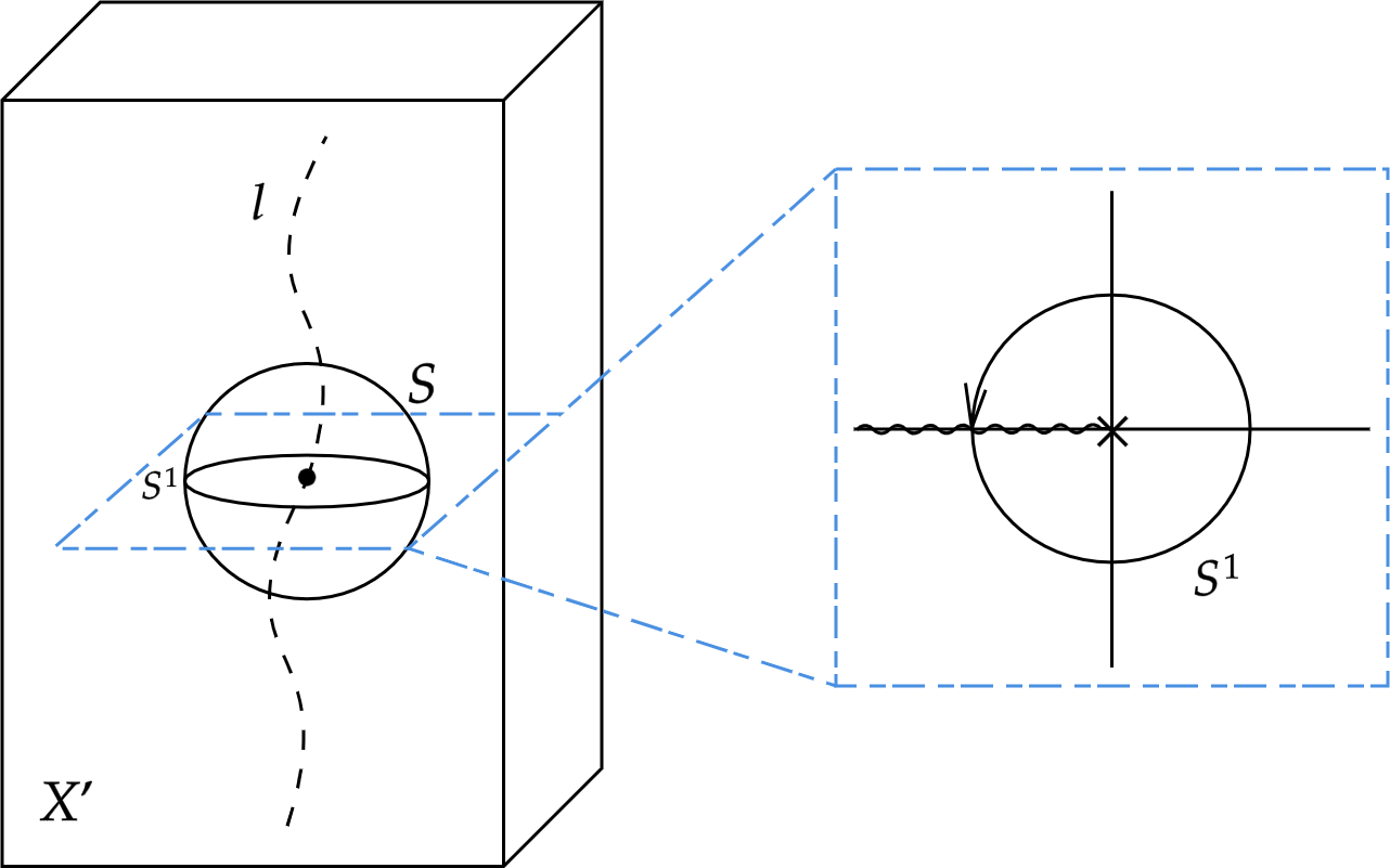
Figure 1: The clutching construction for the monopole. Left: The excised spacetime 4-manifold $X^{\prime}$ and its boundary $\partial X^{\prime}\cong S\times l$. Right: The singularity structure of $\lambda_{1}$ on the equatorial slice $S^{1}$ across $S\cong S^{2}$. If the monopole charge $q_{m}$ is non-trivial, then a branch cut appears.

Any given monopole current $j_{m}$ can thus be inserted by designing the singularity of $\lambda_{1}$; see Fig. 1 (Right). It computes the winding number

$$\int_{S^{1}}d\lambda_{1}=\lambda_{1}(1)-\lambda_{1}(0)\in 2\pi\mathbb{Z},$$

hence the quantized monopole charge $q_{m}\in\mathbb{Z}$ is fixed by topology. In fact, this winding number is precisely the first Chern number $\int_{S}c_{1}(F)$, where the first Chern class $c_{1}(F)=\frac{1}{2\pi}[F]\in H^{2}(X,\mathbb{Z})$ topologically classifies the $U(1)$-bundle on $X$ up to isomorphism. More details can be found in [2].

Remark 2.11.

Given two $U(1)$-bundles $P,P^{\prime}\rightarrow X$ with monopole charges $q_{m},q_{m}^{\prime}$, the tensor bundle $P\otimes P^{\prime}$ has the sum $q_{m}+q_{m}^{\prime}$ as its monopole charge; this is precisely the additive property of characteristic classes [58]

$$c_{1}(P\otimes P^{\prime})=c_{1}(P)+c_{1}(P^{\prime}),$$

and describes the process of monopole fusion. By the clutching construction, we can identify monopole defects with branch points of $L=d\lambda_{1}$ along the equator $S^{1}\subset S^{2}$. As multiple monopoles time-evolve and fuse, a graph is traced out on the cylinder $S^{1}\times l$. The fusion algebra of the Hilbert space of such graph states is known as the (2+1)D Ocneanu’s tube algebra [60, 61, 62].

If we write $d\lambda_{1}=L$ as a generic 1-form, then we see that the anomalous $U(1)$ gauge theory acquires a shift $A\rightarrow A+L$, generating a "$U(1)_{1}$ 1-form symmetry" [23, 24]. We can then follow our previous construction and introduce a 2-form $\Sigma$ as in 2.2.

Resolving the monopole anomaly; 2-gauge structure.

One may treat monopole Maxwell’s theory as a compact $U(1)$ gauge theory equipped with a quantized Gauss law

$$\frac{1}{2\pi}\int_{S}F=0\mod\mathbb{Z},$$

which forces $A\sim A+2\pi$ to be defined only modulo $2\pi\mathbb{Z}$ [56]. Alternatively, however, introducing a 2-gauge structure is in fact the most consistent way to treat the monopole [23, 24].

The idea is to insert a 2-form gauge field $\Sigma$ that absorbs the flux of the magnetic monopole. This is accomplished by the crucial monopole property

$$\int_{S}\Sigma=\int_{S}F,\qquad\forall\text{ closed 2-surfaces }S\subset X^{\prime},$$ (2.41)

which states that the quantized monopole charge ${q}_{m}\in\mathbb{Z}$ is matched by the 2-form gauge field $\Sigma$. However, the monopole condition (2.41) does not imply the fake-flatness $\Sigma=F$ on the nose, but only up to closed 2-forms. We shall abuse notation and write such closed 2-forms as $dL$, which can in general have a non-trivial integral over the surface $S$.

The curvature $F$ transforms as $F\rightarrow F+dL$ under this 2-gauge/1-form shift symmetry, which can in fact change the monopole charge if $L$ has non-trivial periods

$$\frac{1}{2\pi}\int_{S^{2}}dL$$

on the boundary 2-sphere $S^{2}\subset S^{2}\times l=\partial X^{\prime}$. In order to absorb this ambiguity, we must force the 2-form $\Sigma$ to transform as

$$\Sigma\rightarrow\Sigma+dL.$$ (2.42)

On the other hand, recall that the $U(1)$-connection $A$, as well as the gauge parameter $\lambda=\lambda_{0}$, are all regular on the excised 4-manifold $X^{\prime}$, and hence admit an extension into the whole of $X$. As such $F$ — and hence $\Sigma$ — is invariant under a 1-gauge transformation.

Thus the anomalous $U(1)$-gauge theory achieves a mixed 0-form/1-form $U(1)_{1}\times U(1)$ symmetry, governed by a trivial 2-group

$$\mathfrak{I}_{U(1)}=(t=\operatorname{id}:U(1)_{1}\rightarrow U(1),\rhd=1).$$ (2.43)

The action $\rhd=1$ at the group level implies $\rhd=0$ at the algebra level, which allows us to write the transformation law (2.42) as

$$\Sigma\rightarrow\Sigma+dL+\lambda\rhd\Sigma=\Sigma+dL;$$

we have the invariant 2-curvature and the higher Bianchi identity

$$K=d\Sigma\rightarrow d\Sigma+d^{2}L=K,\qquad dK=0.$$

The fake-flatness $F=t\Sigma=\Sigma$ then encodes the monopole condition (2.41), and the 2-curvature $K=\ast j_{m}\neq 0$ can be used to encode the monopole current $j_{m}$ without assuming a violation of Bianchi identity $dF\neq 0$.

Relation to Green-Schwarz anomaly cancellation.

What we have demonstrated is that, to resolve an anomalous 0-form symmetry, we must introduce a 2-group structure with mixed 0- and 1-form symmetry. This is precisely the idea leveraged in [23] in order to implement the Green-Schwarz mechanism of anomaly cancellation in QFT. We describe this procedure briefly in the following.

Consider a field theory with background $U(1)\times U(1)^{\prime}$-symmetry, in which the first copy of $U(1)$ is anomalous in the sense that its associated curvature $F$ has a monopole defect as described above. Here, we use a prime to indicate the other non-anomalous copy $U(1)^{\prime}$, with associated curvature $F^{\prime}$. The anomaly polynomial, which appears under a $U(1)$ transformation of the partition function, takes the form

$$-\int F\wedge F^{\prime}.$$ (2.44)

To cancel this anomaly, we introduce precisely the structure of the 2-group $\mathfrak{I}_{U(1)}$ as above to resolve the monopole anomaly.

By taking the monopole current $\ast j_{m}=dF$ as a source for the 2-curvature anomaly, such that $K=\kappa(A)=dF$, we can solve easily the descent equation (2.25) $\zeta(A,\lambda)=F$. Suppose we source the 2-form connection $\Sigma$ with a 2-form current $J$, and impose the dynamical EOM $F^{\prime}=\ast J$ in the non-anomalous sector, then, performing the modified gauge transformation $\Sigma\rightarrow\Sigma+\zeta(A,\lambda)=\Sigma+F$ on the sourcing term gives

$$\int_{X}\Sigma\wedge\ast J\rightarrow\int_{X}\Sigma\wedge\ast J+\int_{X}F\wedge\ast J\sim\int_{X}\Sigma\wedge\ast J+\int_{X}F\wedge F^{\prime},$$

which cancels exactly the mixed anomaly (2.44) in the partition function. This mechanism allows a consistent gauging of the 0-form symmetry $U(1)\times U(1)^{\prime}$; for more details, see [23, 24]. Note that the underlying 2-group structure is given by

$$t:U(1)_{1}\rightarrow U(1)\times U(1)^{\prime},\qquad t(z)=(z,0),$$

where the first factor $\operatorname{id}:U(1)_{1}\rightarrow U(1)$ is the trivial 2-group $\mathfrak{I}_{U(1)}$ (2.43).

2-Yang-Mills theory; 2-conservation law and mobility restriction.

We now utilize the above concept of monopole anomaly resolution in order to study an anomaly-free version of monopole electrodynamics. By anomaly-free, we mean that the $U(1)$-bundle $P\rightarrow X$ under consideration has trivial first Chern class.

Such a bundle hosts no monopole anomaly, and the Bianchi identity $dF=0$ is satisfied everywhere. In order to introduce a monopole charge, we intend to design a 2-form $\Sigma$ with a non-trivial quantized period,

$$0\neq q_{m}=\frac{1}{2\pi}\int_{S}\Sigma\in\mathbb{Z},\qquad\Sigma=dL,$$ (2.45)

(where the 1-form $L$ has a branch cut as shown in Fig. 1) from an action principle. Recall that, by the clutching construction, the value of the monopole charge is fixed by the singularity structure of $L$.

The goal is therefore to construct an action of a 2-gauge theory that describes the electrodynamics of regular anomaly-free Maxwell’s theory, as well as the monopole configuration of the 2-form connection $\Sigma=dL$. We begin by forming the manifestly invariant quantity $\mathcal{F}=F-\Sigma$ under (regular) 1-form shift symmetry $A\rightarrow A+L^{\prime}$, and write down the Abelian 2-Yang-Mills theory [63]

$$S_{\text{2YM}}[A,\Sigma]=\int_{X}\ast\mathcal{F}\wedge\mathcal{F}=\int_{X}\ast(F-\Sigma)\wedge(F-\Sigma),$$ (2.46)

which has also appeared in the study of topological orders protected by subsystem symmetry [25]. By varying the 2-connection $\Sigma$, we obtain the EOM $\ast(F-\Sigma)=0$, which is nothing but fake-flatness $\mathcal{F}=F-\Sigma=0$. However, in order to have non-trivial monopoles charges, we must consider the off-shell configurations $F\neq\Sigma$. This is because fake-flatness kills the monopole $K=d\Sigma=dF=0$ by the Bianchi identity. Note that we do not expect any issue despite a violation of the fake flatness condition since the theory is Abelian.

In order to have a non-trivial monopole configuration, we must therefore source the 2-connection $\Sigma$. We do something more general here and source both the 1- and 2-connections $A,\Sigma$ individually, with 1- and 2-form currents $j_{e},J$, respectively. This inserts the following terms

$$S_{\text{2cur}}=\int_{X}\ast j_{e}\wedge A+\int_{X}\ast J\wedge\Sigma$$ (2.47)

into $S_{\text{2YM}}$. Intuitively, the 2-form current $J$ should be related in some way to the monopole current $\ast j_{m}$; indeed, upon a variation of $\Sigma$, the sourced action (2.46) together with current contribution (2.47) leads to the EOM

$$\ast(F-\Sigma)=\ast J\implies d\Sigma=-dJ,$$

where we have used the Bianchi identity $dF=0$. By definition, the pure-gauge 2-connection $\Sigma=dL$ has quantized period given by the monopole charge

$$q_{m}=\frac{1}{2\pi}\int_{S}\Sigma=\frac{1}{2\pi}\int_{S\times l}d\Sigma=-\frac{1}{2\pi}\int_{S\times l}dJ,$$

and combined with the definition (2.40) leads to

$$dJ=-\ast j_{m}.$$

This identifies the flux $dJ$ of the 2-form current $J$ with precisely the monopole current. This makes sense, as $J$ sources the 2-connection $\Sigma$ that introduces the monopole.

Remark 2.12.

We emphasize here that the 2-Yang-Mills theory (2.46) is anomaly-free, meaning that it does not have any monopole currents $j_{m}$ as the Bianchi identity $dF=0$ is satisfied. Indeed, the main point of the construction is to source the monopole charge with a 2-form current $J$ without introducing anomalies.

Now to derive the conservation laws of the currents $j_{e},J$, we make gauge transformations on $S_{\text{2YM}}+S_{\text{2cur}}$. A (regular) 0-gauge transformation $A\rightarrow A+d\lambda$ leads to

$$S_{\text{2cur}}\rightarrow S_{\text{2cur}}+\int_{X}\ast j_{e}\wedge d\lambda=S_{\text{2cur}}-\int_{X}\lambda(d\ast j_{e}),$$

which accounts for the conservation $d\ast j_{e}=0$ of the electric current. Suppose now we make the 1-form shift transformation $A\rightarrow A+L^{\prime},\Sigma\rightarrow\Sigma+dL^{\prime}$. The action $S_{\text{2YM}}$ remains invariant, but the sourcing terms acquire

$$S_{\text{2cur}}\rightarrow S_{\text{2cur}}+\int_{X}\ast j_{e}\wedge L^{\prime}+\ast J\wedge dL^{\prime}=S_{\text{2cur}}+\int_{X}(\ast j_{e}-d\ast J)\wedge L^{\prime},$$

which implies the 2-conservation law

$$d\ast J=\ast j_{e}.$$ (2.48)

This implies that the conservation $d\ast J=0$ of the 2-form current $J$ occurs only if $j_{e}=0$ — the 2-form current $J$ is conserved only if isolated charges are immobile, precisely like a dipole. Indeed, (2.48) is also known as a dipole conservation law [25].

This mobility restriction is similar to that for fractons [64, 65]. There had been effort to describe (3+1)D fracton models in the continuum with foliated BF-type field theories [66].

2.5.4 4D topological orders: quasistring defects and surface linking

We have seen in the monopole case above that certain curvature anomalies can be used to represent topological invariants of $X$. There, the first Chern class $c_{1}\in H^{2}(X,\mathbb{Z})$ classifying complex line bundles on $X$ can be represented by the curvature 2-form $F$ through Chern-Weil theory [58, 67].

The topological invariants of $X$ of particular interest are the Stiefel-Whitney classes $w\in H^{\bullet}(X,\mathbb{Z}_{2})$ of the tangent bundle $TX\rightarrow X$, which classifies the framing of $X$ [58, 67]. Our goal in this section is to leverage the structures of a 2-group in order to insert higher-dimensional topological anomalies. Since we shall only be interested in the topological defects of the theory, we assume our structure 2-group $\mathfrak{G}=(V\xrightarrow{0}N,\rhd)$ is skeletal with $t=0$.

Inserting higher-form topological defects.

Let $X$ be a framed 5-manifold with boundary $Y=\partial X$. Given a skeletal 2-group $\mathfrak{G}=(0:V\rightarrow N,\rhd)$, its associated 2-gauge theory encodes the following fake-flatness and 2-flatness conditions,

$$\mathcal{F}=F=0,\qquad\mathcal{G}=K-\kappa(A)=0,$$

such that the 1- and 2-connections $(A,\Sigma)$ are in a sense "decoupled". Excitations of the theory can be inserted separately by modifying these EOMs [19]

$$\mathcal{F}=f_{2}\in C^{2}(X,\mathbb{R})\otimes\mathfrak{n},\qquad\mathcal{G}=g_{3}\in C^{3}(X,\mathbb{R})\otimes V,$$

where $C^{\bullet}(X,\mathbb{R})$ denote the complex of $\mathbb{R}$-valued differential cochains on $X$. The worldvolumes of the excitations in $Y$ are determined by the restrictions of the cochains $f_{2},g_{3}$ to $Y$ via Poincaré duality [58]

$$\operatorname{PD}:C^{n}(Y,\mathbb{R})\rightarrow C_{4-n}(Y,\mathbb{R}).$$

More explicitly, if $\iota:Y\hookrightarrow X$ is the inclusion of the 4d boundary, then $\operatorname{PD}(\iota^{*}g_{3})$ is a 1-cycle (a worldline) on $Y$ [25]. Similarly, the 2-cycle $\operatorname{PD}(\iota^{*}f_{2})$ can be interpreted as the worldsheet of a string-like excitation [19, 30].

One of the key points demonstrated in section 2.5.3 (and later in section 3.3.2) is that the characteristic classes contribute as "anomalous" topological excitations, or defects, of the theory. As such our goal is to construct a 2-gauge structure hosting the Stiefel-Whitney classes $w_{2},w_{3}$ as defects. Following [18, 19], we work directly with flat discrete 2-connections that exhibit the Stiefel-Whitney classes as topological defects.

The construction of gauge fields that capture topological defects gives rise to an invertible topological quantum field theory (TQFT), such as Yetter theory [40] or Dijkgraaf-Witten theory [18, 62]. These objects make an appearance in high-energy physics [68, 24] and condensed matter physics [69, 20], as it is common lore [6] that anomalies in QFTs are in a very general sense topological.

Remark 2.13.

One can expect that topological features are relevant in quantum gravity. Indeed, if we accept that quantum gravitational fluctuations allow for topology change, then one way to keep track of them is to use a 2-group structure, through a 2-connections with non-trivial topological configurations, such as those that we shall construct below. Another interesting direction would be to formulate the 2-group field theory [70] which generates topological amplitudes to non-trivial (ie. non-zero Postnikov class) crossed-modules. We shall leave this to a future work.

Discrete flat 2-connections.

Recall that flat $G$-connections on $Y$ can be uniquely assigned, up to homotopy, through the choice of a classifying map $f:X\rightarrow BG$, where $BG$ is the classifying space of $G$ [58]. A similar situation occurs for 2-groups; in the following, we shall focus on the discrete skeletal 2-group $\mathcal{D}(\mathbb{Z}_{2})\equiv(\mathbb{Z}_{2}\xrightarrow{0}\mathbb{Z}_{2},\rhd=0)$.

The classifying space $B\mathcal{D}(\mathbb{Z}_{2})$ can be constructed from a Postnikov tower [18, 19, 9], such that a discrete flat $\mathcal{D}(\mathbb{Z}_{2})$-connection can be assigned onto $X$ through the choice of a classifying map [18, 19, 71]

$$f:X\rightarrow B\mathcal{D}(\mathbb{Z}_{2}),$$

up to homotopy. Now a simple computation in group cohomology [72] yields a non-trivial generator $[\kappa]\in H^{3}(\mathbb{Z}_{2},\mathbb{Z}_{2})\cong\mathbb{Z}_{2}$, which allows us to define

$$w_{3}=f^{*}[\kappa]$$ (2.49)

as the pullback by $f$. This equation uniquely determines $f$ up to homotopy [18].

The discrete 2-gauge structure we aim for should then have as EOMs on the boundary $Y=\partial X$:

$$F=dA=0,\qquad K=f^{*}\kappa=\kappa(A)=w_{3},$$

where $(A,\Sigma)$ denotes a flat $\mathcal{D}(\mathbb{Z}_{2})$-connection defined by the classifying map $f$. We have thus defined a discrete 2-connection that realizes the third Stiefel-Whitney class $w_{3}$ as a 2-curvature anomaly.

These EOMs can be recovered from a 2-BF type action based on the 2-group $\mathcal{D}(\mathbb{Z}_{2})$. For this, we introduce the Lagrange multipliers $b\in C^{2}(Y,\mathbb{Z}_{2}),c\in C^{1}(Y,\mathbb{Z}_{2})$ on the boundary $Y=\partial X$, and we recover a 2-BF action similar to (2.26),

$$S_{\text{2BF}}=\frac{1}{2}\int_{Y}b\cup F+c\cup(K-f^{*}\kappa)=\frac{1}{2}\int_{Y}b\cup dA+c\cup(d\Sigma-w_{3}),$$

where $\cup$ is the cup product on $\mathbb{Z}_{2}$-valued cochains [58].

We would like to introduce the second Stiefel-Whitney class $w_{2}$ in a similar way, but this time associated to the 1-curvature $F$. One cannot do that directly since 2-group $\mathcal{D}$ is skeletal and so by construction we have $F=0$. We can, however, insert it as a dual 1-curvature anomaly, that is as a source from the 1-gauge theory inherited from the dual 2-group $\mathcal{D}^{*}$ gauge theory. By appending a term

$$\frac{1}{2}\int_{Y}w_{2}\cup\Sigma$$

to the 2-BF theory $S_{\text{2BF}}$, we achieve the EOM upon a variation of $\Sigma$:

$$\tilde{F}=dc=w_{2},$$

which can be interpreted as an anomaly in the dual curvature (2.27). After going on-shell of $F=0$, the boundary action then reads [30]

$$S_{\text{2BF}}\sim S_{\partial}=\frac{1}{2}\int_{Y}c\cup(d\Sigma-w_{3})+w_{2}\cup\Sigma.$$ (2.50)

Notice that we have not assumed integral lifts — ie. an integral cohomology class $c_{2}\in H^{2}(X,\mathbb{Z})$ such that $c_{2}\mod 2=w_{2}$ — exist for either $w_{2}$ or $w_{3}$. Indeed, an integral lift exists for $w_{2}$ only when $w_{3}=0$ [29]!

Due to the closure $dw_{n}=0$ of the Stiefel-Whitney classes, we have

$$\frac{1}{2}d\left(c\cup(d\Sigma-w_{3})+w_{2}\cup\Sigma\right)=\frac{1}{2}(dc\cup w_{3}+w_{2}\cup d\Sigma)\sim w_{2}\cup w_{3},$$

where we have used the EOMs for $c$ and $\Sigma$. This means that $S_{\partial}$ can be interpreted as the boundary action of a bulk 5d symmetry-protected topological (SPT) phase

$$\mathcal{C}_{\text{5d}}=\int_{X}w_{2}\cup w_{3},$$ (2.51)

protected by the global 2-group symmetry $\mathcal{D}(\mathbb{Z}_{2})$. Conversely, we may begin with the action (2.51), and interpret the cochains $c,\Sigma$ and their EOMs as trivializations for $w_{2},w_{3}$ on the boundary $Y=\partial X$ [29, 30].

Remark 2.14.

A topological order is symmetry-protected if it describes a gapped phase that is topologically trivial when the symmetry is ignored [73]. In general, an invertible topological order can be interpreted as being hosted on the boundary of a bulk symmetry protected topological (SPT) order, through the mechanism of anomaly inflow/resolution [31, 29].

The above general formalism of using a 2-group structure to capture higher-degree topological invariants has appeared in [18, 19]. The action (2.50) and topological order (2.51) specifically has also been studied in [30], and we shall follow this reference and provide a brief summary of its interesting properties in the remainder of this section., The new insight we provided here is the understanding that the EOM $dc=w_{2}$ appears as a dual EOM for the associated 2-$BF$ theory, which implies that the boundary action (2.50) is characterized by an underlying 2-Drinfel’d double associated to $\mathcal{D}(\mathbb{Z}_{2})$; see Remark 2.8. This shall be made explicit in an upcoming work by the authors.

Framed submanifolds; the fermionic quasistring order.

The order (2.51), $\mathcal{C}_{\text{5d}}$, hosts on $Y$ a (closed) "magnetic" quasistring described by $\Sigma$, and an "electric" dual quasiaprticle described by $c$; we denote by $l^{2},l$ their worldvolumes, respectively. To understand what this means geometrically, we recall that a framing is equivalent to a trivialization of the normal bundle [58], and that the Stiefel-Whitney classes $w_{n}$ keep track of the twists in the framing of $(n-1)$-dimensional embedded submanifolds [30]; see Fig 2.

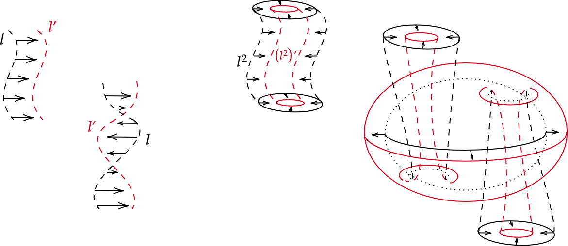
Figure 2: Twists in the framing structure: the "push-offs" [30] $l^{\prime},(l^{2})^{\prime}$ of the worldvolumes $l,l^{2}$ along their framings are shown in red. Left: The quasiparticle described by $c$, and a twist of its 1-dimensional worldline $l$. Right: The quasistring described by $\Sigma$, and a twist in its 2-dimensional worldsheet $l^{2}$.

$\Sigma,c$ are fields associated to $w_{3},w_{2}$, hence they "detect" respectively, via their values $\pm 1$ on $1,2$-dimensional submanifolds $l,l^{2}\subset X$, twists in the framings of $l,l^{2}$. Those that exhibit this twisting are interpreted as the worldvolumes of the quasi-particle/string.

Remark 2.15.

Many topological orders, such as the 5d quasistring order $\mathcal{C}_{\text{5d}}$ (2.51) here, are cobordism invariants [29, 31, 30, 6]. This means, in particular, that they all vanish $\mathcal{C}_{\text{5d}}=0$ on bounding 5-manifolds. Bordism invariants are elements of the (framed) bordism group $\Omega^{O}_{\ast}$ [74, 69]. They constitute the non-perturbative part of the anomalies that appear in QFTs [6, 31].

The $w_{2}w_{3}$ gravitational anomaly.

One of the most interesting properties of the order $\mathcal{C}_{\text{5d}}$ given in (2.51) is that it detects a gravitational anomaly [29, 30]: taking $Y=\mathbb{C}P^{2}$ and $X_{\varphi}=Y\times_{\varphi}S^{1}$ and the diffeomorphism $\varphi:(z_{1},z_{2})\mapsto(\bar{z}_{1},\bar{z}_{2})$, where the $z_{i}$ are coordinates on $\mathbb{C}P^{2}$, one has $\mathcal{C}_{\text{5d}}=1\mod 2$, which evaluates to a non-trivial anomaly

$$\mathcal{Z}(Y)=(-1)^{\mathcal{C}_{\text{5d}}}=\exp\left(i\pi\int_{X_{\varphi}}w_{2}\cup w_{3}\right)=-1$$ (2.52)

associated to the diffeomorphism $\varphi$.

In fact, this mapping torus $X_{\varphi}=\mathbb{C}P^{2}\times_{\varphi}S^{1}$ generates the framed bordism group $\Omega^{O}_{5}$; in other words, any other 5-dimensional cobordism $X$ that evaluates to $-1$ in (2.52) is cobordant to the mapping torus $X_{\varphi}$ of $Y=\mathbb{C}P^{2}$.

The partition function $\mathcal{Z}$ in (2.52) defines an invertible fermionic topological quantum field theory (TQFT) $\mathcal{Z}$ [6, 31, 69] given by the order $\mathcal{C}_{\text{5d}}$. In general, whether a TQFT is bosonic or fermionic is determined by the self-braiding statistics of its defects [73, 19].

In dimensions $\geq 3$, point-like defects can be braided such that their worldlines $l,l^{\prime}$ are linked, as shown in Fig. 2 (Left). This procedure is encoded by a linking number $\operatorname{lk}(l,l^{\prime})$, which changes by 1 upon a twist [74]. In dimensions $\geq 4$, one can braid worldsheets $l^{2},(l^{2})^{\prime}$ with each other, as shown in Fig. 2 (Right). We also have a corresponding surface-linking number $\operatorname{lk}(l^{2},(l^{2})^{\prime})$, which also changes by 1 upon a twist [30].

The spin-TQFT $\mathcal{Z}$ exhibiting the gravitational anomaly given in (2.52) defines a topological order with fermionic quasiparticle and quasistring excitations [29, 30]. What this means is that the Wilson loop and surface operators corresponding to these quasiparticles and quasistrings are accompanifed by the following phases,

$$(-1)^{\operatorname{lk}(l,l^{\prime})}\qquad(-1)^{\operatorname{lk}(l^{2},(l^{2})^{\prime})},$$ (2.53)

in the quantum theory; if these phases are present, then the exictations are bosonic.

3 Gauging the 2-gauge

Recall from section 2 that we noticed that the curvature $F$ was invariant under a shift $\alpha$, a closed form with value in the center of $\mathfrak{g}$. Generalizing this to an arbitrary shift led to the "gauging the 1-gauge". This approach extends to the 2-gauge case. Indeed, given we have a covariantly closed 2-form $\sigma$ such that $d_{A}\sigma=0$, we see that the 2-curvature $K=d_{A}\Sigma$ is (strongly) invariant under the shift $\Sigma\rightarrow\Sigma+\sigma$.

In the following, we shall gauge this global symmetry by taking this shift to be an arbitrary 2-form $\sigma\in\Omega^{2}(X)\otimes\mathfrak{h}$. In this sense, we will make the 2-curvature gauge datum.

3.1 From shifting the 2-connection to a Lie algebra 2-crossed module

3.1.1 Shifting the 2-connection

Consider a 2-connection shift $\Sigma\rightarrow\Sigma+\sigma$ by an arbitrary 2-form $\sigma$. The 2-curvature $K$ then transforms accordingly

$$K\rightarrow K^{\prime}=d_{A}\Sigma+d_{A}\sigma,$$

hence the 3-curvature $K\rightarrow K^{\prime}\neq K$ fails to be invariant, even on-shell of the fake-flatness condition. To remedy this, we introduce a 3-form gauge field by

$$\Gamma\equiv K^{\prime}-K=d_{A}\sigma.$$ (3.1)

Following the same reasoning as previously, the shift we are performing does not have to come from the same algebra $\Sigma$ is valued in. We consider a 2-form $\mathcal{L}\in\Omega^{2}(X)\otimes\mathfrak{i}$ valued in another Lie algebra $\mathfrak{i}=\operatorname{Lie}I$, and replace (3.1) by a "pure gauge" connection 3-form $\Gamma=d_{A}\mathcal{L}$.

Repeating the same steps as before, we may expect the existence of another crossed-module $\mathfrak{S}=(t^{\prime}:\mathfrak{i}\rightarrow\mathfrak{h},\bar{\rhd})$ such that the shift transformation on the 2-connection

$$\Sigma\rightarrow\Sigma+t^{\prime}\mathcal{L},\qquad t^{\prime}\mathcal{L}=\sigma$$

becomes a "3-gauge transformation" parameterized by $\mathcal{L}\in\Omega^{3}(X)\otimes\mathfrak{i}$. This yields yet another invariant fake curvature quantity, called the 2-fake curvature

$$\mathcal{G}\equiv K-t^{\prime}(\Gamma),$$

and the associated 2-fake-flatness condition $K=t^{\prime}\Gamma$. Notice once again that the 2-curvature anomaly $K=\kappa$ can now be absorbed as a part of the 3-connection $\Gamma$ — we shall make this statement precise in section 3.2.2.

Since $K$ is valued in $\operatorname{ker}t$ on-shell of the fake-flatness condition $\mathcal{F}=0$, enforcing also the 2-fake-flatness condition implies $\operatorname{ker}t=\operatorname{im}t^{\prime}$, i.e. $t\circ t^{\prime}=0$. We thus obtain an exact Lie algebra complex

$$\mathscr{G}:\mathfrak{i}\xrightarrow{t^{\prime}}\mathfrak{h}\xrightarrow{t}\mathfrak{g},$$ (3.2)

for which $t^{\prime}:\mathfrak{i}\rightarrow\mathfrak{h}$ is a crossed-module. Here, $\mathfrak{g}$ acts on both $\mathfrak{h}$ and $\mathfrak{i}$, denoted respectively by $\rhd$ and $\rhd^{\prime}$, under which the maps $t,t^{\prime}$ are both $\mathfrak{g}$-equivariant — meaning that the following diagram, which is a generalization of (2.4),

commutes, where $\operatorname{Der}\mathfrak{g}$ denotes the space of derivations of the Lie algebra $\mathfrak{g}$.

3.1.2 3-curvature and 3-Bianchi identity

3-curvature.

Let us define the 3-curvature $T=d_{A}\Gamma$ in the naïve way. With the exactness $\operatorname{im}t^{\prime}=\operatorname{ket}t$ of the complex (3.2) in mind, as well as on-shell of the 2-fake-flatness condition $t^{\prime}\Gamma=K$, we see that

$$t^{\prime}(T)=d_{A}(t^{\prime}(\Gamma))=d_{A}K=((t\Sigma)\wedge^{\rhd}\Sigma)|_{\operatorname{ker}t}.$$

If the Peiffer identity for the part $t:\mathfrak{h}\rightarrow\mathfrak{g}$ of (3.2) holds, then this term coincides with $[\Sigma\wedge\Sigma]|_{\operatorname{ker}t}$ as computed in (2.11), which vanishes. This is the 2-Bianchi identity.

However, we can also consider the case where the Peiffer identity does not hold, so that $t:\mathfrak{h}\rightarrow\mathfrak{g}$ is no longer necessarily a crossed-module, but merely a precrossed-module. This means that only the first Peiffer condition (equivariance) is satisfied, and $(ty)\rhd y^{\prime}$ does not coincide with the bracket $[y,y^{\prime}]$ on $\mathfrak{h}$ as $(t\cdot)\rhd\cdot$ is in general not skew-symmetric.

To treat the term $(t\Sigma)\wedge^{\rhd}\Sigma|_{\operatorname{ker}t}$, we invoke the exactness of the complex (3.2) to write it as the image of some quantity $\{\Sigma\wedge\Sigma\}_{\text{Pf}}$ under $t^{\prime}$. This quantity is defined by the Peiffer lifting map $\{\cdot,\cdot\}_{\text{Pf}}:\mathfrak{h}^{2\otimes}\rightarrow\mathfrak{i}$, which satisfies

$$t^{\prime}\{y,y^{\prime}\}_{\text{Pf}}=-((ty^{\prime})\rhd y)|_{\operatorname{ker}t},\qquad\forall y,y^{\prime}\in\mathfrak{h}.$$ (3.3)

In other words, $\{\cdot,\cdot\}_{\text{Pf}}$ lifts $((t\cdot)\rhd\cdot)|_{\operatorname{ker}t}$ along $t^{\prime}$ up to $\mathfrak{i}$. If we wish for the 3-curvature to be valued in $\operatorname{ker}t^{\prime}\subset\mathfrak{i}$, similar to how the 2-curvature $K$ is valued in $\operatorname{ker}t\subset\mathfrak{h}$, we must replace $T$ by the modified 3-curvature $\mathcal{H}$,

$$\mathcal{H}=d_{A}\Gamma+Q_{\Sigma},\qquad Q_{\Sigma}=\{\Sigma\wedge\Sigma\}_{\text{Pf}}.$$ (3.4)

This extra quadratic term $Q_{\Sigma}$ is an artifact of forgoing the Peiffer identity for $t:\mathfrak{h}\rightarrow\mathfrak{g}$ but, importantly, should not itself be considered an anomaly. We shall elaborate more on this in section 3.2.2.

3-Bianchi identity.

Given the modified 3-curvature (3.4), we can assess what properties we should consider to have if we want to have a 3-Bianchi identity to hold (on shell of the fake-flatness condition $t\Sigma=F$),

$$d_{A}\mathcal{H}=d_{A}(T+Q_{\Sigma})=0.$$ (3.5)

We compute, assuming that there would be no violation of 1-Bianchi identity,

$$d_{A}\mathcal{H} = F\wedge^{\rhd^{\prime}}\Gamma+\{K\wedge\Sigma\}_{\text{Pf}}+\{\Sigma\wedge K\}_{\text{Pf}}$$

$$= t\Sigma\wedge^{\rhd^{\prime}}\Gamma+\{K\wedge\Sigma\}_{\text{Pf}}+\{\Sigma\wedge K\}_{\text{Pf}}$$

Demanding that the last quantity is zero, on-shell of the 2-flatness condition, imposes a relation between $\{\cdot,\cdot\}_{\text{Pf}}$, $t$, $t^{\prime}$ and $\rhd^{\prime}$, which appears when we consider a Lie algebra 2-crossed-module. Such relation is one of the 2-Peiffer conditions, which we shall see below.

Remark 3.1.

It would be possible to investigate the notion of a "weak 2-crossed module" by violating the 1-Bianchi identity. This can be accomplished by relaxing the Jacobi identity on $\mathfrak{g}$ in the definition of a 2-crossed-module. We shall not delve on this here, however, as this requires much more elaboration.

3.1.3 Lie algebra 2-crossed-module

We are now ready to define what a 2-crossed-module is. Let $\mathfrak{g},\mathfrak{h},\mathfrak{i}$ be Lie algebras.

Definition 3.1.

[33] The 3-term algebra complex $\mathscr{G}$ in (3.2), equipped with the bilinear map $\{\cdot,\cdot\}_{\text{Pf}}:\mathfrak{h}^{\otimes 2}\rightarrow\mathfrak{i}$, is a 2-crossed module if and only if

• the action $\mathfrak{h}\bar{\rhd}\mathfrak{i}$ defined by $y\bar{\rhd}z\equiv-\{t^{\prime}z,y\}_{\text{Pf}}$ makes $\mathfrak{S}=(t^{\prime}:\mathfrak{i}\rightarrow\mathfrak{h},\bar{\rhd})$ into a crossed-module,

• the 2-Peiffer conditions are satisfied

  $$\{t^{\prime}z,y\}_{\text{Pf}}+\{y,t^{\prime}z\}_{\text{Pf}} = -ty\rhd^{\prime}z,$$

  $${[z,z^{\prime}]} = \{t^{\prime}z,t^{\prime}z^{\prime}\}_{\text{Pf}},$$

  for all $y\in\mathfrak{h}$ and $z,z^{\prime}\in\mathfrak{i}$,

• the 3-Jacobi identities is satisfied

  $$\{y,[y^{\prime},y^{\prime\prime}]\}_{\text{Pf}} = \{(y,y^{\prime})_{\text{Pf}},y^{\prime\prime}\}_{\text{Pf}}-\{(y,y^{\prime\prime})_{\text{Pf}},y^{\prime}\}_{\text{Pf}},$$

  $$\{[y,y^{\prime}],y^{\prime\prime}\}_{\text{Pf}} = \{ty\rhd y^{\prime},y^{\prime\prime}\}_{\text{Pf}}-\{ty^{\prime}\rhd y,y^{\prime\prime}\}_{\text{Pf}}$$

  $$+\{y^{\prime},(y,y^{\prime\prime})_{\text{Pf}}\}_{\text{Pf}}-\{y,(y^{\prime},y^{\prime\prime})_{\text{Pf}}\}_{\text{Pf}}$$

  for all $y,y^{\prime},y^{\prime\prime}\in\mathfrak{h}$, where $(\cdot,\cdot)_{\text{Pf}}\equiv t^{\prime}\{\cdot,\cdot\}_{\text{Pf}}$ is the $\operatorname{im}t^{\prime}=\operatorname{ker}t$-valued Peiffer pairing, and

• the lifting condition (3.3), is satisfied. Both $\{\cdot,\cdot\}_{\text{Pf}}$ and $(\cdot,\cdot)_{\text{Pf}}$ are $\mathfrak{g}$-equivariant.

Note $\{\cdot,\cdot\}_{\text{Pf}}$ is in general not skew-symmetric.

It was proposed [33] that this 2-crossed-module serves as the structure of a principal 3-gauge bundle $\mathscr{P}\rightarrow X$.

In this case, we have the 1-gauge connection $A$ with value in $\mathfrak{g}$, the 2-connection $\Sigma$ with value in $\mathfrak{h}$ and the 3-connection $\Gamma$ with value in $\mathfrak{i}$. The modified 3-curvature satisfies the 3-Bianchi identity thanks to the first of the 2-Peiffer conditions. We have indeed that

$$t\Sigma\wedge^{\rhd^{\prime}}\Gamma=-\{t^{\prime}\Gamma,\Sigma\}_{\text{Pf}}-\{\Sigma,t^{\prime}\Gamma\}_{\text{Pf}},$$

which together with the 2-fake flatness insures that the 3-Bianchi is satisfied. We now study the gauge transformation structure.

3.2 Gauge transformations and descent equation

We now turn to the 3-gauge transformations on the fields $(A,\Sigma,\Gamma)$ in question. Let us fix the notation

$$\lambda\in\Omega^{0}(X)\otimes\mathfrak{g},\qquad L\in\Omega^{1}(X)\otimes\mathfrak{h},\qquad\mathcal{L}\in\Omega^{2}(X)\otimes\mathfrak{i}$$

for the 0-, 1- and 2-form gauge parameters in the theory. We shall derive the 3-gauge transformation rules, under the principle that the curvature quantities

$$\mathcal{F}=F-t\Sigma,\qquad\mathcal{G}=K-t^{\prime}\Gamma,\qquad\mathcal{H}=d_{A}\Gamma+Q_{\Sigma}$$

transform covariantly. We shall recover the results given in [75].

3.2.1 Gauge transformations

We begin by assuming for simplicity that the 2-gauge sector, involving the fields $(A,\Sigma)$, should retain the same transformation laws under the 2-gauge parameters $(\lambda,L)$ as we have derived in section 2.4.

1-gauge transformations.

We utilize the action of $\mathfrak{g}$ on the two other Lie algebras $\mathfrak{h},\mathfrak{i}$. Since in the 2-gauge context, $K=d_{A}\Sigma\rightarrow K-\lambda\rhd K$ is covariant, the 3-form $\Gamma$ must also transform covariantly,

$$t^{\prime}\Gamma\rightarrow t^{\prime}\Gamma-\lambda\rhd t^{\prime}\Gamma=t^{\prime}\Gamma-t^{\prime}(\lambda\rhd^{\prime}\Gamma)\implies\Gamma\rightarrow\Gamma-\lambda\rhd^{\prime}\Gamma,$$

in order to achieve the covariance of the 2-fake-curvature

$$\mathcal{G}=K-t^{\prime}\Gamma\rightarrow\mathcal{G}^{\lambda}=\mathcal{G}-\lambda\rhd\mathcal{G}.$$

Moreover, due to the $\mathfrak{g}$-equivariance of the Peiffer lifting map $\{\cdot,\cdot\}_{\text{Pf}}$, the modified 3-curvature (3.4) also achieves the covariant transformation

$$\mathcal{H}=d_{A}\Gamma+Q_{\Sigma}\rightarrow\mathcal{H}^{\lambda}=\mathcal{H}-\lambda\rhd^{\prime}\mathcal{H},$$ (3.6)

as desired.

2-gauge transformations.

For this case, we utilize (2.18) for the 2-gauge transformation law of $K$, with the caveat that the Peiffer identity for $t:\mathfrak{h}\rightarrow\mathfrak{g}$ is no longer necessarily satisfied. As such, we write the $[L\wedge L]$ term in the 2-gauge transformation $\Sigma^{L}$ as $tL\wedge L$. This yields

$$K\rightarrow K^{L}=K+tL\wedge^{\rhd}\Sigma^{L}+F\wedge^{\rhd}L.$$

This indicates the transformation property

$$t^{\prime}\Gamma\rightarrow t^{\prime}\Gamma-tL\wedge^{\rhd}\Sigma^{L}-t\Sigma\wedge^{\rhd}L,$$

such that we achieve the desired covariance

$$\mathcal{G}=K-t^{\prime}\Gamma\rightarrow\mathcal{G}^{L}=\mathcal{G}-\mathcal{F}\wedge^{\rhd}L.$$ (3.7)

Using the lifting condition (3.3) for the Peiffer pairing $(\cdot,\cdot)_{\text{Pf}}=t^{\prime}\{\cdot,\cdot\}_{\text{Pf}}$, we have

$$-tL\wedge^{\rhd}\Sigma^{L}=(\Sigma^{L}\wedge L)_{\text{Pf}}=t^{\prime}\{\Sigma^{L}\wedge L\}_{\text{Pf}},\qquad-t\Sigma\wedge^{\rhd}L=(L\wedge\Sigma)_{\text{Pf}}=t^{\prime}\{L\wedge\Sigma\}_{\text{Pf}},$$

which allows us to deduce the 2-gauge transformation

$$\Gamma\rightarrow\Gamma^{L}=\Gamma+\{\Sigma^{L}\wedge L\}_{\text{Pf}}+\{L\wedge\Sigma\}_{\text{Pf}}$$

for $\Gamma$, provided the 1-Bianchi identity is satisfied (ie. $K$ is valued in $\operatorname{ker}t=\operatorname{im}t^{\prime}$).

A direct computation with this 2-gauge transformation law for $\Sigma$ and $\Gamma$ then produces [75]

$$\mathcal{H}\rightarrow\mathcal{H}^{L}=\mathcal{H}+\{\mathcal{G}^{L}\wedge L\}_{\text{Pf}}+\{L\wedge\mathcal{G}\}_{\text{Pf}}\sim\mathcal{H},$$

which is indeed invariant on-shell of the 1- and 2-fake-flatness conditions $\mathcal{F},\mathcal{G}=0$.

3-gauge transformations.

We expect that a 3-gauge transformation should be parameterized by a 2-form, $\mathcal{L}$, in $\mathfrak{i}$. Hence we naturally posit that $A$ is invariant, $A\rightarrow A^{\mathcal{L}}=A$, and hence so is the 1-curvature $F\rightarrow F^{\mathcal{L}}=F$.

For the remaining fields $\Sigma,\Gamma$, we follow the above gauging the gauge argument and induce a shift transformation

$$\Sigma\rightarrow\Sigma^{\mathcal{L}}=\Sigma+t^{\prime}\mathcal{L},\qquad\Gamma\rightarrow\Gamma^{\mathcal{L}}=\Gamma+d_{A}\mathcal{L}.$$

Recall that the product of a $\mathfrak{g}$-valued form with a $\mathfrak{i}$-valued form is performed through the action $\rhd^{\prime}$.

We now compute that the 2-curvature transforms as (note the $\mathfrak{g}$-equivariance of $t^{\prime}$)

$$K\rightarrow K^{\mathcal{L}}=K+d_{A}t^{\prime}\mathcal{L}=K+t^{\prime}d_{A}\mathcal{L},$$

which gives rise to the invariance of the 2-fake-curvature

$$\mathcal{G}\rightarrow\mathcal{G}^{\mathcal{L}}=\mathcal{G}.$$ (3.8)

Furthermore, as $tt^{\prime}=0$ and $F$ is unchanged, we see that the fake-curvature $\mathcal{F}=F-t\Sigma$ is in fact also invariant under the 3-gauge.

Now performing a 3-gauge transformation on the modified 3-curvature $\mathcal{H}$ gives

$$\mathcal{H}\rightarrow\mathcal{H}^{\mathcal{L}}=\mathcal{H}+F\wedge^{\rhd^{\prime}}\mathcal{L}+\{t^{\prime}\mathcal{L}\wedge\Sigma\}_{\text{Pf}}+\{\Sigma\wedge t^{\prime}\mathcal{L}\}_{\text{Pf}}+\{t^{\prime}\mathcal{L}\wedge t^{\prime}\mathcal{L}\}_{\text{Pf}},$$

for which we may employ the 2-Peiffer conditions (recall $\mathcal{L}$ is a 2-form)

$$\{t^{\prime}\mathcal{L}\wedge\Sigma\}_{\text{Pf}}+\{\Sigma\wedge t^{\prime}\mathcal{L}\}_{\text{Pf}}=-t\Sigma\wedge^{\rhd^{\prime}}\mathcal{L},\qquad\{t^{\prime}\mathcal{L}\wedge t^{\prime}\mathcal{L}\}_{\text{Pf}}=[\mathcal{L}\wedge\mathcal{L}]=0$$

to deduce the covariance

$$\mathcal{H}\rightarrow\mathcal{H}^{\mathcal{L}}=\mathcal{H}+\mathcal{F}\wedge^{\rhd^{\prime}}\mathcal{L}\sim\mathcal{H}.$$ (3.9)

The modified 3-curvature $\mathcal{H}$ is thus invariant on-shell of the fake-flatness condition $\mathcal{F}=0$ [75] (which we recall is preserved by the exactness $tt^{\prime}=0$ of the complex (3.2)).

In summary, we have the following 3-gauge transformations

$$\lambda : \begin{cases}A\rightarrow A^{\lambda}=A+d_{A}\lambda\\ \Sigma\rightarrow\Sigma^{\lambda}=\Sigma-\lambda\rhd\Sigma\\ \Gamma\rightarrow\Gamma^{\lambda}=\Gamma-\lambda\rhd^{\prime}\Gamma\end{cases},$$

$$L : \begin{cases}A\rightarrow A^{L}=A+tL\\ \Sigma\rightarrow\Sigma^{L}=\Sigma+d_{A}L+\frac{1}{2}tL\wedge L\\ \Gamma\rightarrow\Gamma^{L}=\Gamma+\{\Sigma^{L}\wedge L\}_{\text{Pf}}+\{L\wedge\Sigma\}_{\text{Pf}}\end{cases},$$

$$\mathcal{L} : \begin{cases}A\rightarrow A^{\mathcal{L}}=A\\ \Sigma\rightarrow\Sigma^{\mathcal{L}}=\Sigma+t^{\prime}\mathcal{L}\\ \Gamma\rightarrow\Gamma^{\mathcal{L}}=\Gamma+d_{A}\mathcal{L}\end{cases}$$ (3.10)

that generate the gauge symmetry $\operatorname{Gau}_{3}$ of our 3-gauge theory. This was also derived in [33, 75].

Compatibility between the 3-gauge transformations.

Importantly, it was noted in [33] that 2-gauge transformations $L$ do not generate a subalgebra when the Peiffer bracket is not zero. Indeed, they commute only up to a 3-gauge transformation,

$$[(0,L_{1},0),(0,L_{2},0)]=(0,0,\mathcal{L}_{12}),\qquad\mathcal{L}_{12}=2(\{L_{1}\wedge L_{2}\}_{\text{Pf}}-\{L_{2}\wedge L_{1}\}_{\text{Pf}}).$$ (3.11)

On the other hand, the computations

$$[(\lambda_{1},0,0),(\lambda_{2},0,0)]=([\lambda_{1},\lambda_{2}],0,0),\qquad[(0,0,\mathcal{L}_{1}),(0,0,\mathcal{L}_{2})]=0,$$

as well as the obvious results

$$[(\lambda,0,0),(0,L,0)]=(0,\lambda\rhd L,0),\qquad[(\lambda,0,0),(0,0,\mathcal{L})]=(0,0,\lambda\rhd^{\prime}\mathcal{L}),$$

allow us to completely characterize the 3-gauge group as

$$\operatorname{Gau}_{3}=\mathscr{E}\rtimes(\Omega^{0}(X)\otimes\mathfrak{g}),\qquad 0\rightarrow\Omega^{2}(X)\otimes\mathfrak{i}\rightarrow\mathscr{E}\rightarrow\Omega^{1}(X)\otimes\mathfrak{h}\rightarrow 0.$$

Here, $\mathscr{E}$ can be seen as a sort of central extension of the 2-gauge by the 3-gauge according to (3.11).

3.2.2 3-curvature anomaly and its first descendant

The goal in this section is to study the anomaly $\tau$ of the modified 3-curvature $\mathcal{H}$, as well as derive conditions on its descendant. In the absence of the 2-Bianchi anomaly, the modified 3-curvature $\mathcal{H}$ is valued in $\operatorname{ker}t^{\prime}$, and so must the anomaly $\tau$. We shall see that, analogous to section 2.4.2, given that the 3-curvature anomaly $\tau$ takes a particular form, then it is related to the classifying cohomology class of the underlying 2-crossed-module $\mathscr{G}$ under consideration.

We wish to insert $\tau$ which preserves the covariance of the anomaly EOM $\mathcal{H}=\tau$ under the 3-gauge transformations (3.10). This tells us that $\tau$ should transform convariantly under a 3-gauge transformation, identically to how $\mathcal{H}$ transforms (3.9). Therefore, on-shell of the fake-flatness condition $\mathcal{F}=0$, the 3-curvature anomaly $\tau$ should be invariant under a 3-gauge transformation, meaning that it must be 2-shift-invariant $\tau(A,\Sigma)=\tau(A,\Sigma+t^{\prime}\mathcal{L})$. As such, $\tau$ can only be a function on $\mathfrak{g}$ and $\operatorname{coker}t^{\prime}=\mathfrak{h}/\operatorname{im}t^{\prime}$. Notice that the quadratic term depends only on $\operatorname{coker}t^{\prime}$, as $Q_{t\mathcal{L}}=[\mathcal{L}\wedge\mathcal{L}]=0$ by the 2-Peiffer condition.

We now examine the conditions for which the 3-curvature anomaly EOM $\mathcal{H}=\tau$ is covariant under 2-gauge transformations. Once again, the covariance of $\mathcal{H}$ (3.2.1) implies that $\tau=\tau(A)$ cannot depend on the 2-connection $\Sigma$, and must be shift-invariant $\tau(A)=\tau(A+tL)$. This casts $\tau$ as a $\operatorname{ker}t^{\prime}$-valued, degree-4 function of $\operatorname{coker}t$, which is precisely the data of a 4-cocycle representative of the Lie algebra cohomology class $[\tau]\in H^{4}(\operatorname{coker}t,\operatorname{ker}t^{\prime})$ that classifies the 2-crossed-module $\mathscr{G}$ up to equivalence [36, 10, 9]; see also Remark A.1 in Appendix A.3.

Twisted 1-gauge transformations.

Going back to the anomaly EOM $\mathcal{H}=\tau(A)$ for the modified 3-curvature, we have shown that $\tau$ is a function of $\operatorname{coker}t=\mathfrak{g}/\operatorname{im}t$ valued in $\operatorname{ker}t$. This puts us in an identical situation as the 2-curvature anomaly $\kappa(A)$.

With the 1-gauge transformations remaining, we suppose the 1- and 2-form connections $(A,\Sigma)$ transform as usual, and define the first descendant $\xi(A,\lambda)$ of $\tau(A)$ as a twisted 1-gauge transformation in the 3-connection satisfying the descent equation,

$$\Gamma\rightarrow\Gamma+\lambda\rhd^{\prime}\Gamma+\xi(A,\lambda),\qquad d_{A^{\lambda}}\xi(A,\lambda)=\tau(A^{\lambda})-\lambda\rhd^{\prime}\tau(A),$$

such that the covariance of $\mathcal{H}$, (3.6), gives

$$\mathcal{H}^{\lambda}=\mathcal{H}+\lambda\rhd^{\prime}\mathcal{H}=\tau(A^{\lambda}).$$

Here, the first descendant of the 3-gauge $\xi(A,\lambda)\in\Omega^{3}(X)\otimes\operatorname{ker}t^{\prime}$ is a 3-form, in contrast to the 2-form $\zeta(A,\lambda)$ encountered in section 2.4.2.

With $\tau$ and $\xi$ valued in $\operatorname{ker}t^{\prime}$, this twisted gauge transformation does not conflict with the covariance of the modified 3-curvature $\mathcal{H}$ above. Moreover, due to the exactness $tt^{\prime}=0$ of the complex (3.2), the 3-gauge descendant $\xi$ is independent from any 2-curvature anomaly.

3.2.3 2-curvature anomaly and first descendant as 3-gauge data

It is more accurate to say that there is only the 3-gauge descendant here, as the 2-curvature anomaly $K=\kappa(A)$ can be understood as a particular 3-connection via the 2-fake-flatness condition $t^{\prime}\Gamma=K$. Indeed, as $K=d_{A}\Sigma$, we can consider $\Gamma=d_{A}\mathcal{L}(A)$ as a pure 3-gauge whose gauge parameter depends on the 1-connection $A$, with $t^{\prime}=\operatorname{id}$ the identity.

Note that $\kappa=\kappa(A)$ can only depend on the 1-connection $A$, which is unaffected by the 3-gauge transformation. Hence locally, we can perform a 3-gauge shift parametrized by $\mathcal{L}$ (which could depend on $A$) in order to remove the 2-curvature anomaly,

$$K-\kappa(A)\rightarrow K+d_{A}\mathcal{L}(A)-\kappa(A)=K,$$

which introduces a gauge-fixing of the 3-connection to a pure gauge $\Gamma=d_{A}\mathcal{L}(A)$. With this choice understood, we now make a 3-gauge transformation followed by a 1-gauge transformation on the 2-connection

$$\Sigma\xrightarrow{\mathcal{L}}\Sigma+\mathcal{L}\xrightarrow{\lambda}\Sigma+\lambda\rhd\Sigma+\mathcal{L}+\mathcal{L}^{\lambda},$$

where we have kept the transformation $\mathcal{L}\xrightarrow{\lambda}\mathcal{L}+\mathcal{L}^{\lambda}$ implicit, as $\mathcal{L}=\mathcal{L}(A)$ now depends on $A$.

In the opposite order, we have

$$\Sigma\xrightarrow{\lambda}\Sigma+\lambda\rhd\Sigma\xrightarrow{\mathcal{L}}\Sigma+\mathcal{L}+\lambda\rhd(\Sigma+\mathcal{L})=\Sigma+\lambda\rhd\Sigma+\mathcal{L}+\lambda\rhd\mathcal{L}.$$

The difference is the expression

$$\mathcal{L}^{\lambda}-\lambda\rhd\mathcal{L},$$

which upon taking the gauge-transformed covariant derivative $d_{A^{\lambda}}$ yields

$$d_{A^{\lambda}}\mathcal{L}^{\lambda}-d_{A^{\lambda}}(\lambda\rhd\mathcal{L})=(d_{A}\mathcal{L})^{\lambda}-\lambda\rhd d_{A}\mathcal{L}=\kappa(A^{\lambda})-\lambda\rhd\kappa(A).$$

This is nothing but the descent equation (2.25) satisfied by the first descendant $\zeta(A,\lambda)$ of the 2-curvature anomaly $\kappa(A)$, if we take

$$\zeta(A,\lambda)=\mathcal{L}^{\lambda}-\lambda\rhd\mathcal{L}.$$

This leads to the identification with the commutator

$$[(0,0,\mathcal{L}),(\lambda,0,0)]=(0,0,\zeta(A,\lambda)).$$ (3.12)

In other words, the 2-curvature anomaly $\kappa(A)$ arising from a Postnikov class can be absorbed by a pure 3-gauge, while its descendant can be absorbed by the commutator (3.12), thereby embedding a non-trivial 2-gauge theory into an anomaly-free 3-gauge theory. This is the spirit of anomaly resolution, and we shall see this in action in section 3.3.2.

3.3 Applications

In this section, we discuss concrete examples in which 3-gauge structures naturally arise.

3.3.1 3-BF theory

The simplest topological action to consider is once again an action implementing merely the constraints — namely, the 1-, 2-fake-flatness and the flat 3-curvature conditions — as equations of motion (EOM). Such a theory has been studied in detail in [33], and we follow their treatment here as well.

Action and EOMs.

As previously, we fix a 2-crossed-module $\mathscr{G}=\mathfrak{i}\xrightarrow{t^{\prime}}\mathfrak{h}\xrightarrow{t}\mathfrak{g}$, and we introduce the dual spaces $\mathfrak{i}^{*},\mathfrak{h}^{*},\mathfrak{g}^{*}$ of linear functionals on respectively the Lie algebras $\mathfrak{i},\mathfrak{h},\mathfrak{g}$. We denote their pairing forms collectively by $\langle\cdot,\cdot\rangle$. We begin by introducing Lagrange multipliers $B\in\Omega^{d-2}\otimes\mathfrak{g}^{*},C\in\Omega^{d-3}\otimes\mathfrak{h}^{*},D\in\Omega^{d-4}(X)\otimes\mathfrak{i}^{*}$ implementing the aforementioned conditions.

The 3-$BF$ action (also called the BFCGDH action, but we shall not use this name for obvious reasons) without any 3-curvature anomalies is then

$$S_{\text{3BF}}=\int_{X}\langle B\wedge\mathcal{F}(A,\Sigma)\rangle+\langle C\wedge\mathcal{G}(A,\Sigma,\Gamma)\rangle+\langle D\wedge\mathcal{H}(A,\Sigma,\Gamma)\rangle,$$ (3.13)

in which $\mathcal{F}=F-t\Sigma,\mathcal{G}=d_{A}\Sigma-t^{\prime}\Gamma$, and $\mathcal{H}=d_{A}\Gamma+Q_{\Sigma}$ is the modified 3-curvature. Recall these curvature quantities are covariant, (2.18), (3.6)-(3.9). For $d=3$, the 3-$BF$ theory reduces to a 2-$BF$ theory, since the dual field $D$ does not exist.

The first set of EOMs is

$$\delta B\Rightarrow\mathcal{F}=0,\qquad\delta C\Rightarrow\mathcal{G}=0,\qquad\delta D\Rightarrow\mathcal{H}=0,$$

which implement precisely the 1-, 2-fake-flatness and 3-flatness conditions, respectively. Since we also have to vary $A,\Sigma$ and the 3-connection $\Gamma$, in addition to the maps $\Delta,t^{*}$ given in section 2.5.1, we introduce

$$\Delta^{\prime}:\mathfrak{i}^{\otimes 2}\rightarrow\mathfrak{g} \,,\, \langle D\wedge A\wedge^{\rhd^{\prime}}\Gamma\rangle=-\langle\Delta^{\prime}(D\wedge\Gamma)\wedge A\rangle,$$

$$\Omega:\mathfrak{i}\rightarrow\mathfrak{h}, \,,\, \langle D\wedge Q_{\Sigma}\rangle=-\langle\Omega(D)\wedge\Sigma\rangle,$$

$$t^{\prime*}:\mathfrak{h}\rightarrow\mathfrak{i}, \,,\, \langle C\wedge t^{\prime}\Gamma\rangle=\langle t^{\prime*}C\wedge\Gamma\rangle,$$

and also the dual action

$$\langle z,x\rhd^{\prime}z^{\prime}\rangle=\langle x\rhd^{\prime*}z,z^{\prime}\rangle$$

for all $z,z^{\prime}\in\mathfrak{i},X\in\mathfrak{g}$. Notice that $\Omega(D)$ is a ($d-2$)-form.

These yield the dual EOMs

$$\delta A \Rightarrow dB+[A\wedge B]^{*}-\Delta(C\wedge\Sigma)-\Delta^{\prime}(D\wedge\Gamma)=0,$$

$$\delta\Sigma \Rightarrow dC+A\wedge^{\rhd^{*}}C-t^{*}B-\Omega(D)=0,$$

$$\delta\Gamma \Rightarrow dD+A\wedge^{\rhd^{\prime*}}D-t^{\prime*}C=0.$$

If we define, in addition to $\tilde{F}=dC+A\wedge^{\rhd^{*}}C$ and $\tilde{K}=dB+[A\wedge B]^{*}$ as in (2.27), the quantity

$$\tilde{T}=dD+A\wedge^{\rhd^{\prime*}}D,$$

we see that these dual EOMs read

$$(d-1) \tilde{K}=\Delta(C\wedge\Sigma)+\Delta^{\prime}(D\wedge\Gamma),$$-form:

$$(d-2) \tilde{F}=t^{*}B+\Omega(D),$$-form:

$$(d-3) \tilde{T}=t^{\prime*}C.$$-form: (3.14)

Symmetries of the action.

Similar to the 2-gauge case, we also acquire 3-gauge transformations in the dual fields $B,C,D$. These have been developed in [33], but to write them down, we must introduce yet more structures.

We define the following maps

$$\omega_{1,2}:\mathfrak{i}\times\mathfrak{h}\rightarrow\mathfrak{h} \Rightarrow \langle z,\{y,y^{\prime}\}_{\text{Pf}}\rangle=-\langle\omega_{1}(z,y),y^{\prime}\rangle=-\langle\omega_{2}(z,y^{\prime}),y\rangle,$$

$$\mathcal{Y}:\mathfrak{i}\times\mathfrak{h}^{\otimes 2}\rightarrow\mathfrak{g} \Rightarrow \langle z,\{x\rhd y,y^{\prime}\}_{\text{Pf}}\rangle=-\langle\mathcal{Y}(z,y,y^{\prime}),x\rangle,$$

for each $Z\in\mathfrak{i},Y,Y^{\prime}\in\mathfrak{h},X\in\mathfrak{g}$. Notice that since $\{y,y\}_{\text{Pf}}=Q_{y}$, we have

$$\langle\omega_{1,2}(z,y),y\rangle=\langle\Omega(z),y\rangle,$$

and that $\omega_{1}\neq\omega_{2}$ or $\omega_{1}\neq-\omega_{2}$ in general, as $\{\cdot,\cdot\}_{\text{Pf}}$ is not symmetric or skew-symmetric.

The dual 3-gauge transformations are given by [33]

$$\lambda : \begin{cases}B\rightarrow B^{\lambda}=B+[\lambda,B]\\ C\rightarrow C^{\lambda}=C+\lambda\rhd C\\ D\rightarrow D^{\lambda}=D+\lambda\rhd^{\prime}D\end{cases},$$

$$L : \begin{cases}B\rightarrow B^{L}=B+\Delta(C\wedge L)+\mathcal{Y}(D\wedge L\wedge L)\\ C\rightarrow C^{L}=C+\omega_{1}(C\wedge L)+\omega_{2}(C\wedge L)\\ D\rightarrow D^{L}=D\end{cases},$$

$$\mathcal{L} : \begin{cases}B\rightarrow B^{\mathcal{L}}=B+\Delta^{\prime}(D\wedge\mathcal{L})\\ C\rightarrow C^{\mathcal{L}}=C\\ D\rightarrow D^{\mathcal{L}}=D\end{cases},$$ (3.15)

which preserves the 3-$BF$ action (3.13) when performed alongside the 3-gauge transformations (3.10).

Analogous to the 2-gauge case in section 2.5.1, we see that the 3-gauge group $\operatorname{Gau}_{3}=\mathscr{E}\rtimes\Omega^{1}(X)\otimes\mathfrak{g}$ acts on the dual fields $B,C,D$. As such, one would expect the data $(\Delta,\Delta^{\prime},\omega^{1,2},\mathcal{Y})$ emergent from the dual EOMs (3.14) to define a strict coadjoint representation $\operatorname{ad}^{*}:\mathscr{G}\rightarrow\operatorname{End}\mathscr{G}^{*}[2]$ on the dual three-term algebra complex

$$\mathscr{G}^{*}[2]:\mathfrak{g}^{*}\xrightarrow{t^{*}}\mathfrak{h}^{*}\xrightarrow{t^{\prime*}}\mathfrak{i}^{*},\qquad t^{\prime*}t^{*}=(tt^{\prime})^{*}=0.$$

Unfortunately, the duality theory of Lie 3-algebras has not been studied in the literature, and the notion of a "3-Manin triple" has yet to be developed. We leave this task to the ambitious reader.

Remark 3.2.

Notice that, in order for the dual fields $B,C,D$ to have the right degree-count to serve as a "dual 3-connection" $(D,C,B)$, we must have $d=\operatorname{dim}X=5$ in contrast to the case in 2-BF theory (where $d=4$). As such, it seems that the "3-Manin triple" most naturally provides the symmetry structure of the 3-BF theory in 5D.

3.3.2 Anomaly resolution: 2-monopoles and the string 2-crossed-module

The key idea explained in section 2.5.3 is that a curvature anomaly (ie. the monopole) can be absorbed by introducing a higher-gauge structure. In this section, we demonstrate this also for a 2-curvature anomaly arising from a Postnikov class, by introducing a 3-gauge structure to resolve it. We shall take $G$ to be a connected, simply connected, compact simple Lie group of rank $\geq 3$, eg. the spin group $G=\operatorname{Spin}(n)$ for $n\geq 3$.

Loop and path algebras.

We define the based path group $PG$ of $G$ as the space of maps $\gamma:[0,1]\rightarrow G$ with basepoint $\gamma(0)=1\in G$ fixed. $PG$ is equipped with the compact-open topology, and group multiplication is defined point-wise

$$(\gamma\gamma^{\prime})(\tau)=\gamma(\tau)\gamma^{\prime}(\tau),\qquad\gamma,\gamma^{\prime}\in PG,$$

where $\tau\in[0,1]$. As a manifold, $PG$ fits in the principal path fibration

$$\Omega G\hookrightarrow PG\xrightarrow{\pi}G\rightarrow\ast,\qquad\pi(\gamma)=\gamma(1)$$

over $G$, where $\Omega G$ is the loop group over $G$ defined as the space of maps $\alpha:S^{1}\rightarrow G$ with a distinguished basepoint $\alpha(0)=\alpha(1)=1$.

By passing to the Lie algebra, we similarly define the path/loop algebras $P\mathfrak{g},\Omega\mathfrak{g}$ consisting of maps from $[0,1]$ or $S^{1}$ into $\mathfrak{g}$, respectively, with initial values based at $0\in\mathfrak{g}$. The Lie brackets are defined point-wise:

$$[p,p^{\prime}](t)=[p(t),p^{\prime}(t)],\qquad p,p^{\prime}\in P\mathfrak{g},$$

where $t\in[0,1]$, and similarly for the loop algebra $\Omega\mathfrak{g}$. We may without loss of generality rescale the loop $S^{1}$ to have unit geodesic length.

As $G$ is simple, all of its central extensions are trivial. This is not the case, however, for its loop group $\Omega G$. Due to a result of Garland [76, 35], the loop algebra has the Lie algebra cohomology

$$H^{2}(\Omega\mathfrak{g},\mathbb{R})\cong\mathbb{R},$$

whence there is a one-dimensional space of non-trivial central extensions

$$0\rightarrow\mathbb{R}\rightarrow\widehat{\Omega_{k}\mathfrak{g}}\rightarrow\Omega\mathfrak{g}$$ (3.16)

spanned by $k\in\mathbb{R}$, called the affine Lie algebra of $\mathfrak{g}$. Note we may write $\widehat{\Omega_{k}\mathfrak{g}}\cong\Omega\mathfrak{g}\oplus\mathbb{R}$ as vector space.

In order to integrate this algebra extension sequence (3.16) to the group level, it was shown [76] that it must satisfy a certain integrality condition. In particular, the level $k\in\mathbb{Z}$ must be quantized, whence we obtain the group extension sequence

$$1\rightarrow U(1)\rightarrow\widehat{\Omega_{k}G}\rightarrow\Omega G\rightarrow 1$$

called the Kac-Moody extension $\widehat{\Omega_{k}G}$ of level $k$; see [35, 76] for an explicit construction.

The loop model for the string 2-algebra.

As shown in [35] and mentioned in Remark 2.6, the string 2-algebra $\mathfrak{string}_{k}(\mathfrak{g})$ admits a description in terms of a non-trivial crossed-module $\mathfrak{l}_{k}$. We have $\mathfrak{l}_{k}=(t:\widehat{\Omega_{k}\mathfrak{g}}\cong\Omega\mathfrak{g}\oplus\mathbb{R}\rightarrow P\mathfrak{g},\rhd)$, and

1. the map $t$ is given by the affine projection $\widehat{\Omega_{k}\mathfrak{g}}\rightarrow\Omega\mathfrak{g}$ composed with the inclusion $\Omega\mathfrak{g}\hookrightarrow P\mathfrak{g}$,

2. $\operatorname{ker}t\cong\mathbb{R}=\{(0,c)\in\Omega\mathfrak{g}\oplus\mathbb{R}\}$, and $\operatorname{coker}t\cong P\mathfrak{g}/\Omega\mathfrak{g}\cong\mathfrak{g}$ is isomorphic to the constant paths,

3. the action is defined as

   $$p\rhd(\ell,c)=([p,\ell],2k\int_{S^{1}}\langle p,\dot{\ell}\rangle),\qquad p\in P\mathfrak{g},\quad(\ell,c)\in\widehat{\Omega_{k}\mathfrak{g}},$$ (3.17)

   whence the induced action $\rhd$ of $\operatorname{coker}t=\mathfrak{g}$ on $\operatorname{ker}t=\mathbb{R}$ is trivial,

4. the Postnikov class $[\kappa]\in H^{3}(\mathfrak{g},\mathbb{R})$ of $\mathfrak{l}_{k}$ is given by the Diximier-Douady class $k[\omega]\in H^{3}(G,\mathbb{Z})$ of $\operatorname{String}_{k}(G)$, where $\omega=\langle\cdot,[\cdot,\cdot]\rangle$ is the fundamental 3-cocycle on $\mathfrak{g}$ [76, 35].

Notice that, in the Chevalley baiss $\{T_{a}\}_{a}$ of $\mathfrak{g}$, the fundamental 3-cocycle $\omega$ gives just the structure constant $f_{ab}^{c}$. The Lie bracket on $\widehat{\Omega_{k}\mathfrak{g}}$ is given by the level-$k$ Kac-Moody extension

$$[(\ell,c),(\ell^{\prime},c^{\prime})]=t(\ell,c)\rhd(\ell^{\prime},c^{\prime})=([\ell,\ell^{\prime}],2k\int_{S^{1}}\langle\ell,\dot{\ell}^{\prime}\rangle),$$

which is also given by the Peiffer identity. We shall focus on the case of level $k=1$ in the following for brevity, but the case for arbitrary values of $k\in\mathbb{Z}$ can be treated identically.

2-gauge structure of the loop model.

With the loop model crossed-module structure $\mathfrak{l}_{1}$, let $(A,\Sigma)$ denote the associated 2-connection with $\Sigma=(\sigma,c)\in\Omega^{2}(X)\otimes(\widehat{\Omega\mathfrak{g}_{1}})\cong(\Omega^{2}(X)\otimes\Omega\mathfrak{g})\oplus\Omega^{2}(X)$, such that $t\Sigma=\sigma$. To derive the 2-curvature anomaly $\kappa(A)$, we compute the 2-curvature as

$$K=d_{A}\Sigma=(d_{A}\sigma,dc+2\int_{S^{1}}\langle A\wedge\dot{\sigma}\rangle),$$

where the prefactor of $2$ comes from the crossed-module action (3.17). On-shell of the fake-flatness condition $\mathcal{F}=F-t\Sigma=0$, we then have

$$K\sim(d_{A}F,dc+2\int_{S^{1}}\langle A\wedge\dot{F}\rangle)=(0,dc+2\int_{S^{1}}\langle A\wedge\dot{F}\rangle),$$

where we have used the 1-Bianchi identity $d_{A}F=0$. Thus we see $K$ is valued in $\operatorname{ker}t$, consistent with what we have discussed in section 2.3.

The 2-form connection is given in components by $\Sigma=(\sigma,c)$ with $\sigma$ valued in $\Omega\mathfrak{g}$, the loop algebra. Since the loops are by definition based at $0\in\mathfrak{g}$, we have in particular $\sigma(1)=\sigma(0)=0$. The fake-flatness condition $F=t\Sigma=\sigma$ then forces $F$ to be valued in the loop algebra $\Omega\mathfrak{g}$ as well:

$$t\Sigma(1)=\sigma(1)=F(1)=dA(1)+\frac{1}{2}[A(1)\wedge A(1)]=0.$$ (3.18)

Notice that this does not necessarily force $A$ to also be valued in $\Omega\mathfrak{g}$, meaning that $A(1)$ does not have to be zero. With this in mind, we compute that

$$\langle\dot{A}\wedge[A\wedge A]\rangle=\frac{1}{3}\frac{\partial}{\partial\tau}\langle A\wedge[A\wedge A]\rangle$$

is a total derivative in the path parameter $\tau\in[0,1]$, whence by a direct computation we have (recalling that $A(0)=0$)

$$\int_{S^{1}}\langle A\wedge\dot{F}\rangle = -\int_{0}^{1}\langle\dot{A}\wedge dA\rangle-\frac{1}{2}\int_{0}^{1}\langle\dot{A}\wedge[A\wedge A]\rangle$$

$$= -\langle A(1)\wedge dA(1)\rangle-\frac{1}{2\cdot 3}\langle A(1)\wedge[A(1)\wedge A(1)]\rangle+\int_{0}^{1}\langle A\wedge d\dot{A}\rangle$$

$$= \frac{1}{3}\langle A(1)\wedge[A(1)\wedge A(1)]\rangle+\int_{0}^{1}\langle A\wedge d\dot{A}\rangle,$$

where we have used (3.18) in the last equality. Using (3.18) once again, we can compute

$$d\int_{0}^{1}\langle A\wedge\dot{A}\rangle = \int_{0}^{1}\langle dA\wedge\dot{A}\rangle-\langle A\wedge d\dot{A}\rangle$$

$$= \langle dA(1)\wedge A(1)\rangle-2\int_{0}^{1}\langle A\wedge d\dot{A}\rangle$$

$$= -\frac{1}{2}\langle A(1)\wedge[A(1)\wedge A(1)]\rangle-2\int_{0}^{1}\langle A\wedge d\dot{A}\rangle,$$

which when recombined with the above expression yields the on-shell 2-curvature

$$K\sim(0,2(\frac{1}{3}-\frac{1}{4})\langle A(1)\wedge[A(1)\wedge A(1)]\rangle+d(c-c_{1}))=(0,\frac{1}{6}\langle A(1)\wedge[A(1)\wedge A(1)]\rangle+dc^{\prime}),$$

where $c_{1}=\int_{0}^{1}\langle A\wedge\dot{A}\rangle$ and $c^{\prime}=c-c_{1}$.

Such exact forms $dc^{\prime}$ can be absorbed into a 2-gauge transformation, hence we achieve the 2-curvature anomaly

$$\kappa(A)\equiv(0,\frac{1}{3!}\langle A(1)\wedge[A(1)\wedge A(1)]\rangle)\in\operatorname{ker}t=\mathbb{R}.$$ (3.19)

This $\kappa(A)=\frac{1}{3!}\omega(A(1),A(1),A(1))$ is given precisely in terms of the fundamental 3-cocycle $\omega=\langle\cdot,[\cdot,\cdot]\rangle$, which is consistent with the fact that the Postnikov class of $\mathfrak{l}_{1}$ coincides with $\omega$ in this case [35].

It is easy to see that $\kappa(A)$ is invariant under 2-gauge transformation $A\rightarrow A+tL$. The terms we acquire are cyclic permutations of

$$\langle A(1)\wedge[A(1)\wedge tL(1)]\rangle+\langle A(1)\wedge[tL(1)\wedge tL(1)]\rangle+\langle tL(1)\wedge[tL(1)\wedge tL(1)]\rangle,$$

which all vanish because $tL$ is valued in $\Omega\mathfrak{g}$, whence $tL(1)=0=tL(0)$.

Since we have a non-trivial $\kappa(A)$, we know from section 2.4.2 that the 1-gauge transformations of $\Sigma$ need to be modified by the first descendant $\zeta(A,\lambda)$. Let $\lambda\in P\mathfrak{g}$ denote a 1-gauge parameter. As $P\mathfrak{g}$ acts trivially on the kernel $\mathbb{R}$, we see that the descent equation (2.25) for $\kappa(A)$ reads

$$d\zeta(A,\lambda)=\kappa(A^{\lambda})-\kappa(A)=\langle d_{A}\lambda(1),[A(1)\wedge A(1)]\rangle$$

to first order in $\lambda$. To find $\zeta(A,\lambda)$ that solves this equation, we first notice that the total skew-symmetry of the pairing form $\langle\cdot,[\cdot,\cdot]\rangle$ implies that

$$\langle[A(1),\lambda(1)]\wedge[A(1)\wedge A(1)]\rangle=-\langle\lambda(1),[A(1)\wedge[A(1)\wedge A(1)]]\rangle=0,$$

which vanishes by the Jacobi identity in $\mathfrak{g}$, hence $\omega(d_{A}\lambda(1),A(1),A(1))=\omega(d\lambda(1),A(1),A(1))$. Now by Leibniz rule and (3.18),

$$d(\omega(\lambda(1),A(1),A(1))) = \omega(d\lambda(1),A(1),A(1))+\langle\lambda(1),[dA(1)\wedge A(1)]\rangle-\langle\lambda(1),[A(1)\wedge dA(1)]\rangle$$

$$= \omega(d\lambda(1),A(1),A(1))+2\langle\lambda(1),[dA(1)\wedge A(1)]\rangle$$

$$= \omega(d\lambda(1),A(1),A(1))-\langle\lambda(1),[[A(1)\wedge A(1)]\wedge A(1)]\rangle,$$

the last term of which vanishes once again by the Jacobi identity in $\mathfrak{g}$, so we can identify $\zeta$,

$$d\zeta(A,\lambda)=d(\omega(\lambda(1),A(1),A(1))),\qquad\zeta(A,\lambda)=\langle\lambda(1),[A(1)\wedge A(1)]\rangle.$$ (3.20)

With such $\zeta$, we do have a proper 2-gauge theory based on the loop model $\mathfrak{l}_{1}$ as discussed in section 2.4.2. We intend now to absorb this 2-curvature anomaly $\kappa(A)$ by describing a 3-gauge theory encoding the same information.

Remark 3.3.

It is interesting to note the striking resemblance between (3.20) and (2.15), the latter of which has appeared in [34]. It is important to note, however, that here we are using a different 2-gauge structure as [34]. In their language, we are in the "unadjusted" case where $K$ transforms covariantly under the adjoint representation of $P\mathfrak{g}$, and $\mathcal{F},\Sigma$ transform independently. In the adjusted case, $K$ is invariant, and $\mathcal{F},\Sigma$ form a $\mathfrak{g}$-multiplet.

2-monopoles and anomalous 2-gauge transformations.

We now cast $\kappa(A)$ as a 2-monopole defect. Let $X$ be a spin 5-manifold. We define the 2-monopole charge conventionally in terms of its current as

$$\tilde{q}_{m}=\frac{1}{8\pi}\int_{W}\ast\tilde{j}_{m},$$ (3.21)

where $\tilde{j}_{m}$ is the 1-form 2-monopole current. In analogy with the monopole case discussed in section 2.5.3, the 2-monopoe current violates the 2-Bianchi identity (2.9) of the loop model 2-gauge theory we have described above.

To see this, we assume $W=V\times l$ decomposes into a closed 3-cycle and the 2-monopole worldline $l$. We introduce an anomalous EOM $dK=\ast\tilde{j}_{m}$ valued in $\operatorname{ker}t=\mathbb{R}$, such that integrating across the 3-cycle $V\subset X$ yields

$$\int_{V}K=\int_{W}dK\neq 0$$

by Stokes’s theorem. This means that the 2-form connection $\Sigma$ acquires a non-trivial 2-holonomy [79, 38] about $V$, which coincides with the 2-monopole charge. On the other hand, the 2-curvature anomaly EOM $K=\kappa(A)$ implies that this 2-holonomy is precisely the period of $\kappa(A)$ in (3.19),

$$\tilde{q}_{m}=\frac{1}{8\pi}\int_{W}\ast\tilde{j}_{m}=\frac{1}{2(4\pi)}\int_{S^{3}}K=\frac{1}{8\pi}\int_{S^{3}}\kappa(A).$$ (3.22)

Such periods are classified by the Postnikov class $[\kappa]=[\omega]\in H^{3}(\mathfrak{g},\mathbb{R})$ (via pullback), therefore if $[\omega]\in H^{3}(\mathfrak{g},\mathbb{Z})\subset H^{3}(\mathfrak{g},\mathbb{R})$ is an integral class, then the 2-monopole charge $\tilde{q}\in\mathbb{Z}$ is quantized.

We recall that the monopole defect studied in section 2.5.3 can be constructed from clutching an anomalous 1-gauge transformation. We do the same for the 2-monopole defect here. By a similar excision trick as in section 2.5.3, we take a tubular neighborhood about the 2-monopole worldline $l$ and remove it from the 5-manifold $X$. This yields a new 5-manifold $X^{\prime}$ with boundary $\partial X^{\prime}\cong S^{3}\times l$, away from which $K$ is regular. We acquire two components $L_{0},L_{1}$ in a 2-gauge transformation

$$\Sigma\rightarrow\Sigma+d_{A}L_{0}+\frac{1}{2}L_{0}^{2}+d_{A}L_{1}+\frac{1}{2}L_{1}^{2},$$

for which $L_{0},L_{1}$ are regular on $X^{\prime}$, but $L_{0}$ can be smoothly extended into $X$ while $L_{1}$ cannot. We call $L_{1}$ singular, and it means, once again, that $d^{2}L_{1}\neq 0$ globally on $X$, hence

$$d^{2}_{A}L_{1}-F\wedge^{\rhd}L_{1}=d^{2}L_{1}\neq 0.$$

From the computations in (2.18), this leads to the anomalous 2-gauge transformation

$$K\rightarrow K+\mathcal{F}\wedge^{\rhd}(L_{0}+L_{1})+d^{2}L_{1}\sim K+d^{2}L_{1},$$

where $\sim$ means going on-shell of the fake-flatness condition $\mathcal{F}=F-t\Sigma=0$.

As $K$ is smooth and regular within $X^{\prime}$, it cannot yield a non-trivial 2-monopole charge. The sole contributor of $\tilde{q}_{m}$ must then come from the anomalous component $L_{1}$:

$$\tilde{q}_{m}=\frac{1}{8\pi}\int_{S^{3}}K\xrightarrow{\sim}\frac{1}{8\pi}\int_{S^{3}}d^{2}L_{1}=\frac{1}{4\pi}\int\limits_{S^{2}=H_{+}\cap H_{-}}dL_{1}\neq 0,$$

where we have used Stokes’s theorem on the two patches $D^{3}\cong H_{\pm}\subset S^{3}$ that cover the 3-sphere. The singular 2-gauge parameter $L_{1}$ has the structure of a "hedghog defect" [5, 2], and its 2-dimensional winding number is identified with $\tilde{q}_{m}$.

Remark 3.4.

The 2-monopole defect, being point-like in 5D, behaves similarly to the 1-monopole in 4d studied in section 2.5.3. In particular, two 2-monopole defects may fuse such that their charges add, corresponding to the additivity

$$\kappa(\mathcal{P}\otimes\mathcal{P}^{\prime})=\kappa(\mathcal{P})+\kappa(\mathcal{P}^{\prime})$$

of the Postnikov classes associated to the 2-gauge bundles $\mathcal{P},\mathcal{P}^{\prime}\rightarrow X$; see [18].

This clutching construction [58] for the 2-monopole allows us to match the 2-curvature anomaly with an anomalous 2-gauge transformation, $\kappa(A)=d^{2}L_{1}$, via (3.22) on the boundary 3-sphere $S^{3}$. Writing $dL_{1}=\mathcal{L}$, we once again see a "2-shift transformation"

$$\Sigma\rightarrow\Sigma+\mathcal{L},$$ (3.23)

manifesting before us, generating a "$U(1)_{2}$ 2-form symmetry". This suggests the 3-gauge structure we should define in order to resolve the anomaly $\kappa(A)$.

Resolving the 2-monopole anomaly; the 3-gauge structure.

We can now introduce a 3-form field $\Gamma$ to absorb the 2-curvature anomaly. This is encoded by the 2-monopole condition

$$\int_{V}\Gamma=\int_{V}K,\qquad\forall\leavevmode\nobreak\ \text{closed 3-surfaces }V\subset X^{\prime},$$ (3.24)

stating that the quantized 2-monopole charge $\tilde{q}_{m}\in\mathbb{Z}$ is matched by the flux of the 3-form $\Gamma$.

If we take $t^{\prime}=\operatorname{id}$ as the identity (strictly speaking an inclusion) as suggested by (3.23) and (3.24), to achieve the exactness $tt^{\prime}=0$ of the complex

$$\mathfrak{i}\xrightarrow{t^{\prime}=\operatorname{id}}\widehat{\Omega_{k=1}\mathfrak{g}}\xrightarrow{t}P\mathfrak{g}$$ (3.25)

we must have $\mathfrak{i}=\operatorname{im}t^{\prime}=\operatorname{ker}t=\mathbb{R}$. This means that $P\mathfrak{g}$ acts trivially $\rhd^{\prime}=0$ on $\mathfrak{i}=\mathbb{R}$, and hence on the $\mathfrak{i}$-valued 3-connection $\Gamma$. Moreover, $\operatorname{ker}t^{\prime}=0$ means that the degree-4 Postnikov class $[\tau]$ for (3.25) is trivial.

As $t^{\prime}:\mathfrak{i}=\mathbb{R}\hookrightarrow\mathfrak{h}=\widehat{\Omega_{1}\mathfrak{g}}$ is an inclusion, we have $t^{\prime}\{\cdot,\cdot\}_{\text{Pf}}=\{\cdot,\cdot\}_{\text{Pf}}$. The lifting condition (3.3) then gives

$$\{(\ell,c),(\ell^{\prime},c^{\prime})\}_{\text{Pf}}=[(\ell,c),(\ell^{\prime},c^{\prime})]|_{\operatorname{ker}t}=2\int_{S^{1}}\langle\ell,\dot{\ell}^{\prime}\rangle$$

for $(\ell,c),(\ell^{\prime},c^{\prime})\in\widehat{\Omega_{1}\mathfrak{g}}\cong\Omega\mathfrak{g}\oplus\mathbb{R}$. Here, $\{\cdot,\cdot\}_{\text{Pf}}$ is skew-symmetric, as can be seen by an integration by parts, but it is not trivial. Equipped with this Peiffer lifting map, the complex (3.25) forms a 2-crossed-module which we call the string 2-crossed-module.

The quadratic form $Q$, however, does vanish when evaluated on forms of even degrees, such as the 2-form connection $\Sigma=(\sigma,c)$,

$$Q_{\Sigma}=\int_{S^{1}}\langle\sigma\wedge\dot{\sigma}\rangle=-\int_{S^{1}}\langle\dot{\sigma}\wedge\sigma\rangle=-Q_{\Sigma},$$

thus the modified 3-curvature $\mathcal{H}=d\Gamma$ coincides with the unmodified 3-curvature. The anomalous EOM $d(K|_{\operatorname{ker}t})=\ast\tilde{j}_{m}$ and the 2-monopole condition (3.24) together identify the integral of $\frac{1}{8\pi}\mathcal{H}$ over the boundary 4-surface $\partial X^{\prime}=W=S^{3}\times l$ with the 2-monopole charge.

In the interior of the 5-manifold $X^{\prime}$, we interpret the 2-monopole condition (3.24) as a 2-fake-flatness condition

$$t^{\prime}\Gamma=K.$$

As $P\mathfrak{g}$ acts trivially on $\mathbb{R}=\operatorname{ker}t=\operatorname{im}t^{\prime}$, we can express the 3-curvature by taking the covariant derivative,

$$\mathcal{H}\sim d_{A}K=d_{A}^{2}\Sigma=F\wedge^{\rhd}\Sigma=([F\wedge\sigma],2\int_{S^{1}}\langle F\wedge\dot{\sigma}\rangle).$$

If we now go on-shell of the fake-flatness condition $\mathcal{F}=0$, we then have the 3-flatness condition

$$\mathcal{H}\sim([F\wedge F],2\int_{S^{1}}\langle F\wedge\dot{F}\rangle)=(0,\langle F(1)\wedge F(1)\rangle)=0,$$ (3.26)

where we recall that fake-flatness $F=\sigma$ implies $F$ is valued in $\Omega\mathfrak{g}$, which forces $F(1)=0$. The fake-flatness, 2-fake-flatness and 3-flatness conditions are therefore mutually consistent, and the fields $(A,\Sigma,\Gamma)$ define a flat 3-connection based on (3.25) in the interior of $X^{\prime}$.

Remark 3.5.

What about near the boundary $W=\partial X^{\prime}$? By construction, $W$ contains a tubular neighborhood of the 2-monopole worldline $l$, at which the field $\Sigma$ is singular. The 3-curvature $\mathcal{H}$ then receives a contribution from $d^{2}\Sigma=dK\neq 0$, which on-shell of the 2-fake-flatness and fake-flatness conditions is given precisely by the 2-monopole current $\ast\tilde{j}_{m}$, as we have mentioned previously.

We now demonstrate the gauge invariance of the 2-monopole/2-fake-flatness condition (3.24). First, as $\kappa$ and $K$ are both valued in $\mathbb{R}=\operatorname{ker}t$, the 2-monopole charge is invariant under a 1-gauge transformation $\lambda$. As such $\Gamma$ is also invariant. Next, under the 3-gauge transformation (3.23), the 2-monopole charge $\tilde{q}_{m}$ receives contributions from the possibly non-trivial periods

$$\frac{1}{8\pi}\int_{V}d\mathcal{L}\neq 0,\qquad\mathcal{L}\in\Omega^{3}(X)\otimes\mathfrak{i}.$$

As such, the 3-form connection must transform accordingly

$$\Gamma\rightarrow\Gamma+d\mathcal{L},$$

in order to preserve the 2-monopole condition (3.24).

Recall that the quadratic form $Q$ necessarily vanishes on 2-forms valued in the loop algebra $\Omega\mathfrak{g}$, so under a regular 2-gauge transformation $L_{0}=L$, the 3-curvature $\mathcal{H}$ must be invariant, according to (3.10). This means that the 3-connection $\Gamma$ then transforms by an exact 3-form $d\phi$, $\Gamma\rightarrow\Gamma+d\phi$. On-shell of the 2-fake-flatness condition, we can infer this 2-form $\phi$ from how the 2-curvature $K$ transforms. Indeed, recalling that the 2-curvature $K$ is valued in $\operatorname{ker}t=\mathbb{R}$ on-shell of the fake-flatness condition, we consider the sector $L|_{\operatorname{ker}t}$ and compute

$$K\rightarrow K^{L|_{\operatorname{ker}t}}=K+d^{2}L|_{\operatorname{ker}t}+\frac{1}{2}d[L\wedge L]|_{\operatorname{ker}t}=K+\frac{1}{2}d[L\wedge L]|_{\operatorname{ker}t}.$$

As such, in order to preserve (3.24), the exact 3-form $d\phi$ must be given by $\phi=\frac{1}{2}[L\wedge L]|_{\operatorname{ker}t}$, up to an exact 1-form. To show that this is consistent with (3.10), we compute the 2-gauge transformation

$$\{\Sigma^{L}\wedge L\}_{\text{Pf}}+\{L\wedge\Sigma\}_{\text{Pf}} = \{\Sigma\wedge L\}_{\text{Pf}}+\{L\wedge\Sigma\}_{\text{Pf}}$$

$$+\{d_{A}L\wedge L\}_{\text{Pf}}+\frac{1}{2}\{[L\wedge L]\wedge L\}_{\text{Pf}}\qquad\text{Skew-symmetry of $\{\cdot,\cdot\}_{\text{Pf}}$}$$

$$= \{d_{A}L\wedge L\}_{\text{Pf}}+\frac{1}{2}\{[L\wedge L]\wedge L\}_{\text{Pf}}\qquad\text{Equivariance of $\{\cdot,\cdot\}_{\text{Pf}}$}$$

$$= \frac{1}{2}d_{A}\{L\wedge L\}_{\text{Pf}}+\frac{1}{2}\{[L\wedge L]\wedge L\}_{\text{Pf}}\qquad\text{Jacobi identity}$$

$$= \frac{1}{2}d_{A}\{L\wedge L\}_{\text{Pf}}\qquad\text{Action $\rhd^{\prime}=0$ is trivial on $\mathfrak{i}=\operatorname{ker}t^{\prime}$}$$

$$= \frac{1}{2}d\{L\wedge L\}_{\text{Pf}},$$

which is indeed nothing else than $\phi=\frac{1}{2}\{L\wedge L\}_{\text{Pf}}=\frac{1}{2}[L\wedge L]|_{\operatorname{ker}t}$ by the lifting condition (3.3). This means that we have a fully-fledged 3-gauge theory based on the 2-crossed-module (3.25) in the interior of $X^{\prime}$, as introduced in section 3 and [33].

In summary, we have demonstrated a 3-group analogue of the observation made in [23, 24] and section 2.5.3: an anomalous 2-group (mixed 0- and 1-form) symmetry — in the sense that the 2-Bianchi identity $dK=\ast\tilde{j}_{m}$ is violated by the presence of a 2-monopole — gauges into a 3-group symmetry, which involves 0-, 1- and 2-form symmetries.

3-Yang-Mills theory.

With the 3-gauge structure based on the string 2-crossed-module in hand, we now construct a non-anomalous 3-Yang-Mills theory $S_{\text{3YM}}$ that captures the 2-monopole. (We still consider $k=1$ in the following.)

Analogous to what was done in section 2.5.3, we begin by considering a trivial 2-gauge theory $\mathcal{P}\rightarrow X$ (ie. vanishing Postnikov class $[\kappa]=0$) and $X$ a spin manifold of dimension 5, and insert a non-trivial 2-monopole charge through a 2-form $\mathcal{L}$ that has a non-trivial quantized period,

$$\tilde{q}_{m}=\frac{1}{8\pi}\int_{V}\Gamma\in\mathbb{Z},\qquad d\mathcal{L}=\Gamma.$$ (3.27)

The 2-monopole condition (3.24) allows us to treat $\Gamma$ as a pure-gauge 3-connection, which induces a 3-gauge shift symmetry

$$\Gamma\rightarrow\Gamma+d\mathcal{L}^{\prime}$$

parameterized by regular 2-forms $\mathcal{L}^{\prime}\in\Omega^{2}(X)$. Our fields $(A,\Sigma,\Gamma)$ then acquire the 3-gauge symmetry structure based on the Lie 3-algebra given by the string 2-crossed-module (3.25). The goal is now to construct an action which equations of motion have such shape (3.27) for solution.

We define the 3-Yang-Mills action [80]

$$S_{\text{3YM}}=\int_{X}\ast\mathcal{F}\wedge\mathcal{F}+\ast\mathcal{G}\wedge\mathcal{G},\quad\textrm{with }\mathcal{F}=F-t\Sigma,\quad\mathcal{G}=K-\Gamma.$$ (3.28)

As pairing, we use the non-degenerate pairing on the path and loop algebras

$$\langle p,p^{\prime}\rangle_{P\mathfrak{g}}=\int_{[0,1]}\langle p,p^{\prime}\rangle,\qquad\langle(\ell,c),(\ell^{\prime},c^{\prime})\rangle_{\widehat{\Omega_{1}\mathfrak{g}}}=\int_{S^{1}}\langle\ell,\ell^{\prime}\rangle+cc^{\prime}$$

composed with the Hodge pairing on $\Omega^{\bullet}(X)$. The action (3.28) is the 3-gauge generalization of the higher-Yang-Mills theory developed in [63].

By construction, $S_{\text{3YM}}$ is invariant under 3-gauge transformations (3.10). By varying the 3-gauge $\Gamma$, we obtain the 2-fake-flatness EOM $\mathcal{G}=K-\Gamma=0$. Once again, we see that no non-trivial 2-monopole charge can be introduced on-shell of this EOM, as the original 2-gauge bundle $\mathcal{P}$ was by hypothesis trivial.

To amend this, we source the 1-, 2- and 3-form connections $A,\Sigma,\Gamma$, respectively, with the 1-, 2- and 3-form currents $j,J,\mathcal{J}$. This introduces the following term

$$S_{\text{3cur}}=\int_{X}A\wedge\ast j+\Sigma\wedge\ast J+\Gamma\wedge\ast\mathcal{J}$$

to $S_{\text{3YM}}$ (3.28). The properties of the currents are listed below

Currents	Form degree	Valued in
$j$	1	$P\mathfrak{g}$
$J$	2	$\widehat{\Omega_{1}\mathfrak{g}}\cong\Omega\mathfrak{g}\oplus\mathbb{R}$
$\mathcal{J}$	3	$\mathbb{R}=\operatorname{ker}t$

Upon introducing these currents, a variation of the 3-gauge $\Gamma$ then yields the modified EOM

$$\ast\mathcal{H}=\ast\mathcal{J}\implies d\Gamma=-d\mathcal{J},$$

where we have used the 2-Bianchi identity $d_{A}K=0$ and the fact that $P\mathfrak{g}$ acts trivially on $\operatorname{ker}t$. This makes it possible to identify the flux $d\mathcal{J}$ of the 3-current $\mathcal{J}$ with the 2-monopole and obtain what we sought: as the quantized period of $\mathcal{L}$, we have

$$\tilde{q}_{m}=\frac{1}{8\pi}\int_{V}d\mathcal{L}=\frac{1}{8\pi}\int_{V\times l}d\Gamma=-\frac{1}{8\pi}\int_{V\times l}d\mathcal{J},$$

where $l$ is the worldline. This allows to relate the 2-monopole current $\tilde{j}_{m}$ (3.21) with ${\cal J}$,

$$d\mathcal{J}=-\ast\tilde{j}_{m}.$$

3-conservation laws and higher mobility constraints.

We now derive higher-conservation laws of $S_{\text{3YM}}+S_{\text{3cur}}$ by making 3-gauge transformations.

1. 3-gauge transformation $\mathcal{L}^{\prime}$: the 1-connection $A$ is unaffected, and the sourcing terms introduce

   $$S_{\text{3cur}}\rightarrow S_{\text{3cur}}+\int_{X}\mathcal{L}^{\prime}\wedge\ast J+d\mathcal{L}^{\prime}\wedge\ast\mathcal{J}.$$

   Note that $\mathcal{L}^{\prime}$ (the prime is to distinguish $\mathcal{L}^{\prime}$ from the $\mathcal{L}$ chosen in (3.27)) is valued in $\mathbb{R}=\operatorname{ker}t$; by writing $J=(J_{\ell},J_{c})$ in the $\widehat{\Omega_{1}\mathfrak{g}}\cong\Omega\mathfrak{g}\oplus\mathbb{R}$-components, we achieve

   $$\int_{X}\mathcal{L}^{\prime}\wedge\ast J_{c}+d\mathcal{L}^{\prime}\wedge\ast\mathcal{J}=\int_{X}\mathcal{L}^{\prime}\wedge(\ast J_{c}-d\ast\mathcal{J}),$$

   and hence the first-level conservation law

   $$d\ast\mathcal{J}=\ast J_{c},\qquad J=(J_{\ell},J_{c})\in\Omega\mathfrak{g}\oplus\mathbb{R},\quad{\cal J}\in\mathbb{R}.$$ (3.29)

2. 2-gauge transformation $L$: the sourcing terms introduce

   $$S_{\text{3cur}}\rightarrow S_{\text{3cur}}+\int_{X}tL\wedge\ast j+(d_{A}L+\frac{1}{2}[L\wedge L])\wedge\ast J+d\phi\wedge\ast\mathcal{J},$$

   where $\phi=\frac{1}{2}\{L\wedge L\}_{\text{Pf}}=-\frac{1}{2}L^{2}|_{\operatorname{ker}t}$. To extract conservation laws, we must introduce new operations.

   Using the dual map $t^{*}:P\mathfrak{g}\rightarrow\widehat{\Omega_{1}\mathfrak{g}}$ defined in section 2.5.1, we can rewrite the first term as

   $$-\int_{X}L\wedge t^{*}\ast j.$$

   For the second term, we use an integration by parts and split $L=(L_{\ell},L_{c})$ into $\Omega\mathfrak{g}\oplus\mathbb{R}$-components, such that we have

   $$-\int_{X}L_{\ell}\wedge d_{A}\ast J_{\ell}+\frac{1}{2}\int_{X}[L_{\ell}\wedge L_{\ell}]\wedge\ast J_{\ell}+\frac{1}{2}\int_{X}[L_{c}\wedge L_{c}]\wedge(\ast J_{c}-d\ast\mathcal{J}),$$

   where $[L_{c}\wedge L_{c}]=[L\wedge L]|_{\operatorname{ker}t}$ as in our previous computation. Note the final term vanishes on-shell of (3.29), and hence does not give us anything new.

   Combining these terms, we obtain

   $$-\int_{X}L_{\ell}\wedge(t^{*}\ast j+d_{A}\ast J_{\ell})+\frac{1}{2}\int_{X}[L_{\ell}\wedge L_{\ell}]\wedge\ast J_{\ell}.$$

   If we suppose, for simplicity, that both of these terms individually vanish, then we obtain the set of second-level conservation laws

   $$d_{A}\ast J_{\ell}=-t^{*}\ast j,\qquad\ast J_{\ell}=0.$$ (3.30)

   Of course, the second equation is not imposed if we have kept only the terms linear in $L$ in the 2-gauge transformations.

3. 1-gauge transform $\lambda$: the 3-connection $\Gamma$ is unaffected, and the sourcing terms introduce

   $$S_{\text{3cur}} \rightarrow S_{\text{3cur}}+\int_{X}d_{A}\lambda\wedge\ast j-\lambda\rhd\Sigma\wedge\ast J$$

   $$= S_{\text{3cur}}-\int_{X}\lambda(d_{A}\ast j)-\int_{X}[\lambda,\sigma]\wedge\ast J_{\ell}-2\int_{X}\left[\int_{S^{1}}\langle\lambda,\dot{\sigma}\rangle\right]\wedge\ast J_{c},$$

   where we have used the definition of the action $\rhd$, and written $\Sigma=(\sigma,c)$ in components. Recall we have kept the pairing form $\langle\cdot,\cdot\rangle_{P\mathfrak{g}}$ implicit, such that we have

   $$\int_{X}\lambda(d_{A}\ast j)=\int_{X}\langle\lambda,d_{A}\ast j\rangle_{P\mathfrak{g}}=\int_{X}\int_{[0,1]}\langle\lambda,d_{A}\ast j\rangle$$

   by definition, for instance.

   Due to the cyclic symmetry of the function $\langle\cdot,[\cdot,\cdot]\rangle$, we can write

   $$\langle[\lambda,\sigma]\wedge\ast J_{\ell}\rangle_{\Omega\mathfrak{g}}=\langle[\sigma\wedge\ast J_{\ell}],\lambda\rangle_{\Omega\mathfrak{g}},$$

   which brings the sourcing terms to the form

   $$-\int_{X}\lambda(d_{A}\ast j+[\sigma\wedge\ast J_{\ell}])-2\int_{X}\int_{S^{1}}\langle\dot{\lambda},\sigma\wedge\ast J_{c}\rangle.$$ (3.31)

   Now as $\sigma\in\Omega\mathfrak{g}$, we can perform an integration by parts on the second term of (3.31) without a boundary term,

   $$\int_{S^{1}}\langle\dot{\lambda},\sigma\wedge\ast J_{c}\rangle=-\int_{S^{1}}\langle\lambda,\dot{\sigma}\wedge\ast J_{c}\rangle.$$

   Therefore, (3.31) yields the third-level conservation law

   $$d_{A}\ast j+[\sigma\wedge\ast J_{\ell}]=\dot{\sigma}\wedge\ast J_{c}.$$ (3.32)

   It is clear that the 1-current $j$ is conserved provided the 2-current $J=(J_{\ell},J_{c})=0$ vanishes. This is guaranteed by the condition $J_{\ell}=0$ in (3.30), as well as the requirement that the 3-current $\mathcal{J}$ be conserved, which implies $J_{c}=0$ from (3.29). Therefore the conservation of the 1-current does not impose any new conditions.

A direct consequence of these 3-conservation laws (3.29)-(3.32) is the very interesting mobility constraint. The immobility of the 1-form Kac-Moody charges, $J_{\ell},J_{c}=0$, guarantees that both the 2-form $U(1)_{2}$ and the $PG$ 0-form symmetries are non-anomalous, in the sense that the corresponding 3-,1-currents $\mathcal{J},j$ are conserved,

$$d\ast\mathcal{J}=0,\qquad d_{A}\ast j=0,\qquad d_{A}\ast J_{\ell}=t^{*}(\ast j)=0.$$

The last conservation law states that the 1-current $j$ must be valued in $\operatorname{ker}t^{*}\subset P\mathfrak{g}$. By the rank-nullity theorem, we have

$$\operatorname{ker}t^{*}\cong\operatorname{coker}t=P\mathfrak{g}/\Omega\mathfrak{g}\cong\mathfrak{g},$$

so it appears that the $PG$-charges that descend to those of $G$ can still remain mobile. Therefore, the only charges that are allowed to be mobile are the ones labeled by the 0-form $G$ and the 2-form $U(1)_{2}$ symmetries. Interestingly, despite us starting with the loop model of string 2-algebra, this "mobility data" constitutes precisely the skeletal model [35, 34]; see Remark 2.4.

4 Conclusion

In this paper, we have motivated higher-gauge structures from the gauge theoretic perspective. This was done by the procedure of "gauging the gauge", or equivalently by shifting the $n$-connection in an $n$-gauge theory. We then introduce a $(n+1)$-form connection which is related to the $n$-curvature, so that $n$-curvature has really become gauge data. This allows us to absorb the $n$-curvature anomaly — which may include contributions from topological characteristic classes of degree $n$ — into a $(n+1)$-connection through anomaly resolution. In other words, an anomaly in the $n$-curvature, regardless if it is topological (eg. a monopole) or geometric (eg. a massive particle), can be considered as a choice of the $(n+1)$-gauge (possibly gauge fixed).

We have shown that this anomaly resolution procedure [23, 24] categorifies the $n$-gauge structure, and yields a higher $(n+1)$-gauge theory. Furthermore, the structure $(n+1)$-group in general has the identity as its "top-level" morphism, therefore it is always possible to pick a flat $(n+1)$-gauge theory (ie. hosts no curvature anomalies), at least up to elementary equivalence [36]. We have demonstrated explicitly these concepts in the cases of $n=1$ and $2$.

As such, one may be left with the impression that all $n$-gauge theories for $n<\infty$ can be embedded in an $\infty$-gauge theory [81, 82], which by construction does not have any curvature anomalies. This is true, but in general this categorification procedure cannot continue forever if the spacetime dimension $d=\operatorname{dim}X$ is fixed and finite. It must terminate at the $(d-1)$-form connection, as one does not have the notion of curvature on $X$ for connections of degrees higher than $d-1$.

Moreover, focusing specifically on the $n$-BF theory, one may notice from sections 2.5.1 and 3.3.1 that $n$-BF theory has a dual given by a $n$-gauge theory only when $d=\operatorname{dim}X=n+2$, in which case the symmetries of the $(d-2)$-BF theory is naturally described by an appropriate notion of a "$(d-2)$-Manin triple". Though a $(d-1)$-gauge theory may be well-defined on $X$, there is just no sufficient room for the $n$-Manin triple to fit on a $d$-manifold $X$ if $n>d-2$. This can be rephrased as saying essentially that the dynamics of $k$-dimensional excitations for $k\leq n$ is most naturally embedded in $(n+2)$-dimensions; indeed, one needs two additional ambient dimensions in order to braid excitations, and braiding is one of the central operations that is afforded by a Drinfel’d double [83].

As we have covered a very wide range of topics in physics and mathematics, our treatment may not be completely rigorous. However, we believe to have given sufficient references such that our readers can find further details in them. Nevertheless, our treatment exposes many open problems that may be tackled by future research. In the following, we organize a few of them.

Drinfel’d double and tube algebra.

It is known that the Drinfel’d double $D(SU(2))$ serves as the symmetries of Euclidean 3d $BF$ theory [84]. It is in fact equivalent to the Ocnenau’s tube algebra over $G=SU(2)$ in (2+1)d [61].

On the other hand, we have explained in section 2.5.2 how the structure of the trivial 2-group $\mathcal{I}_{SU(2)}$ arises from Euclidean 3d $BF$ theory when one sources a non-trivial curvature anomaly. The trivial 2-group $\mathcal{I}_{U(1)}$ also arises from resolving the monopole anomaly in section 2.5.3, and we have made the observation in Remark 2.11 that the fusion algebra of these monopoles gives rise to Ocneanu’s tube algebra over $U(1)$ (or over its group characters $\widehat{U(1)}=\mathbb{Z}$). As such, there seems to be an interesting interplay between the trivial 2-group $\mathcal{I}_{G}$ and the Drinfel’d double $D(G)$.

It is known that $D(G)$ in certain circumstances admits a description as an algebra of a certain groupoid [43], and hence one may model the tube algebra as a groupoid algebra. Upon categorification, the (3+1)d tube algebra has been constructed as a 2-groupoid algebra in [62]. It would then be interesting to construct a notion of a "2-Drinfel’d double" (see for example in [85, 86]) that fits with the (3+1)d tube algebra structure.

The classification of (3+1)d SPT phases and the Kitaev model.

The Drinfel’d double $D(G)$ also makes an appearance in condensed matter theory. Specifically for $G=\mathbb{Z}_{2}$, the 2d toric code is defined by the representation category $\operatorname{Rep}(\mathbb{Z}_{2})$ [87]. The effective (2+1)d bulk topological quantum field theory (TQFT) is described by the Kitaev model, whose spectrum of excitations is given by the Drinfel’d centre ${Z}(\operatorname{Rep}(\mathbb{Z}_{2}))$ [20, 88]. The Drinfel’d double $D(\mathbb{Z}_{2})$ is by construction such that

$$\operatorname{Rep}_{D(\mathbb{Z}_{2})}\simeq Z(\operatorname{Rep}_{\mathbb{Z}_{2}}),$$

which allows one to construct a 1-$BF$ $\mathbb{Z}_{2}$-gauge theory with the symmetry $D(\mathbb{Z}_{2})$ that describes the Kitaev model [89].

Similarly, we have seen in section 2.5.4 how to construct a (3+1)d topological order using a discrete 2-group $\mathcal{D}(\mathbb{Z}_{2})$. It hosts a magnetic string and an electric charge defect, both labeled by $\mathbb{Z}_{2}$ [30]. When the emergent electric charge is bosonic, it has been postulated [19] (and rigorously shown [90]) that the effective bulk TQFT is the (3+1)d toric code, described by the Drinfel’d centre $Z(\operatorname{2Rep}_{\mathbb{Z}_{2}})$ of the 2-representation 2-category $\operatorname{2Rep}_{\mathbb{Z}_{2}}$ [20]. Thus, it is reasonable to expect a 2-Drinfel’d double $D$ related to $\mathbb{Z}_{2}$ to manifest such that

$$\operatorname{2Rep}_{D}\simeq Z(\operatorname{2Rep}_{\mathbb{Z}_{2}}).$$ (4.1)

It would be valuable to explicitly construct this categorical equivalence, and study the resulting 2-BF $d$-gauge theory that describes the (3+1)d toric code. This is currently being undertaken by the authors.

In case when the electric charge is fermionic, however, there are two distinct classes of (3+1)d TQFTs [90]. One is the spin $\mathbb{Z}_{2}$-gauge theory described by $Z_{1}(\Sigma{\bf sVect})$, where $\Sigma{\bf sVect}$ is the condensation completion [91] 2-category of supervector spaces. The other is its anomalous version, which hosts the gravitational anomaly (2.52) briefly studied in section 2.5.4. To achieve an effective field theory in these cases would require to develop the notion of quantum 2-groups and their 2-representation theory.

String structures and the $S^{1}$-transgression map in holography.

In section 3.3.2, we gave an example of a 2-crossed-module (3.25) that had arisen through the anomaly resolution procedure for the string 2-algebra in the loop model [35]. We have shown that a consistent, flat 3-gauge theory can be identified in the interior of the excised 5-manifold $X^{\prime}$, thereby categorifying the statement made in [23, 24]: that an anomalous $(n-1)$-form symmetry can be gauged by introducing an $n$-form symmetry.

Near the boundary 4-manifold $W=\partial X^{\prime}$ (which we recall contains the 2-monopole worldline $l$), the 3-curvature $\mathcal{H}$ receives a contribution from the singularity in the 2-form connection $\Sigma$ (see Remark 3.5). On the other hand, if we instead relax the fake-flatness condition to a weaker, differentiated version $\dot{\mathcal{F}}=\dot{F}-t\dot{\Sigma}=0$, then we could obtain another contribution

$$\mathcal{H}\sim(0,\langle F(1)\wedge F(1)\rangle)=\operatorname{tr}(F(1)^{2})$$ (4.2)

aside from the 2-monopole current $\tilde{j}_{m}\neq 0$, as $F(1)$ is no longer required to vanish. This contribution $-4\pi p_{1}\in H^{4}(W,\mathbb{Z})$ is the first Pontrjagyn class of the boundary 4-manifold $\partial X^{\prime}=W$.

In light of (4.2), if we now insist upon the 3-flatness $\mathcal{H}\sim 0$ across the boundary of $X^{\prime}$, then we have

$$\mathcal{H}\sim d^{2}\Sigma+\operatorname{tr}(F(1)^{2})=0\implies\tilde{j}_{m}=4\pi p_{1},$$

which matches the 2-monopole current with the first Pontrjagyn class.

1. Due to the factor of $1/8\pi$ in the definition (3.21) of the 2-monopole charge, the above matching condition implies

   $$\tilde{q}_{m}=\frac{1}{8\pi}\int_{W}\ast\tilde{j}=\frac{1}{2}\int_{W}p_{1}.$$

   It is known that the fractional first Pontrjagyn class $\frac{1}{2}p_{1}\mod\mathbb{Z}$ is an obstruction class for string structures [22]. Therefore, the quantization of the 2-monopole charge $\tilde{q}_{m}\in\mathbb{Z}$ in fact implies the existence of a string structure on the boundary 4-manifold $\partial X^{\prime}=W$.

2. Given the first Chern class $\operatorname{tr}F(1)=0$ vanishes, $p_{1}$ coincides with (minus) the second Chern class $c_{2}$ [67, 76]. This means that the second Chern class controls the 2-monopole defect, analogous to how the first Chern class controls the monopole defect; see section 2.5.3. The procedure of anomaly resolution then allows us to associate the 2-curvature anomaly given by the fundamental 3-cocycle $\omega$ to the second Chern class $c_{2}$ — namely it constructs an inverse to the $S^{1}$-transgression map $H^{4}(G,\mathbb{Z})\rightarrow H^{3}(G,\mathbb{Z})$ [43] seen in the Chern-Simons/Wess-Zumino-Witten holography [21].

As such, it would be important to understand the tower of "higher order fake-flatness conditions" $\frac{d^{n}}{d\tau^{n}}\mathcal{F}=0$ in a more rigorous and complete manner.

Mobility constraints in 3-Yang-Mills theories.

In section 2.5.3, we constructed a 2-Yang-Mills theory based on the trivial 2-group $\mathcal{I}_{U(1)}$ that arises from the anomaly resolution of the magnetic monopole in classical electromagnetism. We derived the higher conservation law (2.48), which imposes a certain mobility constraint for the electric charges provided the dipole charge is conserved. This is consistent with what others have found in the literature [25].

In section 3.3.2, we have also derived a set of new mobility constraints from the higher-conservation laws (3.29)-(3.32) associated to the 3-Yang-Mills theory based on the string 2-crossed-module (3.25). In particular, the central 2-form current $J_{c}$ is rendered immobile, which seems to be consistent with the non-dynamical nature of the central charge in Wess-Zumino-Witten conformal field theory [92, 21]. It would be worthwhile to make this observation into a more concrete statement, and to see what these mobility constraints mean physically for the 3-group charges as a whole. As far as we know, these mobility constraints have never been previously derived, so it seems to be a novel direction to explore.

Appendix A Classification of Lie algebra crossed-modules

In this section we examine the classification of Lie algebra crossed-modules by Lie algebra cohomology, following [36]. Recall that a given two Lie algebras $\mathfrak{h},\mathfrak{g}$ over a fixed field $k$ of characteristic zero, a Lie algebra crossed-module is a map $t:\mathfrak{h}\rightarrow\mathfrak{g}$ and an action $\rhd$ of $\mathfrak{g}$ on $\mathfrak{h}$ such that the following Peiffer conditions

$$t(X\rhd Y)=[X,tY]_{\mathfrak{g}},\qquad tY\rhd Y^{\prime}=[Y,Y^{\prime}]_{\mathfrak{h}}$$ (A.1)

are satisfied for each $Y,Y^{\prime}\in\mathfrak{h},X\in\mathfrak{g}$. Mathematically, it is equivalent to a strict Lie 2-algebra, where the homotopy map $\mu=0$ introduced in the main text vanishes.

Consider the following four-term algebra complex built from the Lie algebra crossed module,

$$0\rightarrow V\hookrightarrow\mathfrak{h}\xrightarrow{t}\mathfrak{g}\rightarrow\mathfrak{n}\rightarrow 0,$$ (A.2)

where $V=\operatorname{ker}t$ and $\mathfrak{n}=\operatorname{coker}t$. Due to the Peiffer identity in (A.1), the Lie algebra $V\subset Z(\mathfrak{h})$ must lie in the centre of $\mathfrak{h}$, and hence is Abelian. It admits an action by $\mathfrak{n}$ induced by the crossed-module action $\rhd$.

Definition A.1.

We say that two crossed modules $t:\mathfrak{h}\rightarrow\mathfrak{g},t^{\prime}:\mathfrak{h}^{\prime}\rightarrow\mathfrak{g}^{\prime}$ with the respective actions $\rhd,\rhd^{\prime}$ are elementary equivalent if

1. $\operatorname{ker}t=\operatorname{ker}t^{\prime}=V$ and $\operatorname{coker}t=\operatorname{coker}t^{\prime}=\mathfrak{n}$,

2. there exists Lie algebra homomorphisms $\phi:\mathfrak{h}\rightarrow\mathfrak{h}^{\prime},\psi:\mathfrak{g}\rightarrow\mathfrak{g}^{\prime}$ compatible with the actions $\rhd,\rhd^{\prime}$ such that

   $$\phi(X\rhd Y)=\psi(X)\rhd^{\prime}\phi(Y)$$

   for all $X\in\mathfrak{g}$ and $Y\in\mathfrak{h}$. Moreover, the diagram

   commutes.

Let us denote the set of elementary equivalence classes of Lie algebra crossed-modules by ${\bf XMod}(\mathfrak{n},V)$.

A.1 Lie algebra cohomology

We first review some basic facts about Lie algebra cohomology, which is a very powerful and important tool for classification of $L_{\infty}$-algebras. We once again follow the treatment of [36].

Let $\mathfrak{n}$ be a Lie algebra over the field $k$ and let $V$ be an Abelian $\mathfrak{n}$-module. Define its differential graded Chevalley-Eilenberg complex

$$(C^{\bullet}(\mathfrak{n},V),d),\qquad C^{p}(\mathfrak{n},V)=\begin{cases}\Lambda(\mathfrak{n}^{p},V)&;p>0\\ V&;p=0\end{cases},$$

where $\Lambda(\mathfrak{n}^{p},V)$ denotes the exterior algebra of alternating forms on $p$-copies of $\mathfrak{n}$ over $V$. The differential $d:C^{p}(\mathfrak{n},V)\rightarrow C^{p+1}(\mathfrak{n},V)$ is given explicitly by

$$dc(x_{0},\dots,x_{p}) = \sum_{i<j}(-1)^{i+j}c([x_{i},x_{j}],x_{0},\dots,\hat{x}_{i},\dots,\hat{x}_{j},\dots,x_{p})$$

$$-\sum_{i=1}^{p}(-1)^{i}x_{i}\rhd c(x_{0},\dots,\hat{x}_{i},\dots,x_{p})$$

for each cochain $c\in C^{p}(\mathfrak{n},V)$, where $\hat{\cdot}$ denotes an omitted element.

Lemma A.1.

$d^{2}=0$.

Proof.

Recall the Cartan formula

$$L_{x}=d\iota_{x}+\iota_{x}d,\qquad x\in\mathfrak{n}$$

where $\iota_{x}:C^{p+1}(\mathfrak{n},V)\rightarrow C^{p}(\mathfrak{n},V)$ is the interior evaluation

$$\iota_{x}:c\mapsto((x_{1},\dots,x_{p})\mapsto c(x,x_{1},\dots,x_{p}))$$

and $L_{x}:C^{p}(\mathfrak{n},V)\rightarrow C^{p}(\mathfrak{n},V)$ is the Lie evaluation

$$L_{x}:c\mapsto((x_{1},\dots,x_{p})\mapsto x\rhd c(x_{1},\dots,x_{p})-\sum_{i}c(x_{1},\dots,[x,x_{i}],\dots,x_{p})),$$

which by construction commutes with $d$. Now let $v\in V=C^{0}(\mathfrak{n},V)$ be a 0-form, then

$$d^{2}v(x_{1},x_{2}) = -dv([x_{1},x_{2}])+x_{1}\rhd dv(x_{2})-x_{2}\rhd dv(x_{1})$$

$$= [x_{2},x_{1}]\rhd v+x_{1}\rhd(x_{2}\rhd v)-x_{2}\rhd(x_{1}\rhd v)=0,$$

which vanishes by the $\mathfrak{n}$-module structure on $V$.

Now let $p>0$ and assume the induction hypothesis: $d^{2}=0$ on $C^{p-1}(\mathfrak{n},V)$. Consider $c\in C^{p}(\mathfrak{n},V)$, then by the Cartan formula

$$d^{2}c(x_{-1},x_{0},x_{1},\dots,x_{p}) = \iota_{x_{-1}}(d^{2}c)(x_{0},x_{1},\dots,x_{p})$$

$$= (L_{x_{-1}}-d\iota_{x_{-1}})dc(x_{0},x_{1},\dots,x_{p})$$

$$= (L_{x_{-1}}d-d(L_{x_{-1}}-d\iota_{x_{-1}})c(x_{0},x_{1},\dots,x_{p})$$

$$= (L_{x_{-1}}d-dL_{x_{-1}}+d^{2}\iota_{x_{-1}})c(x_{0},x_{1},\dots,x_{p})=0,$$

where the first two terms cancel by the property $L_{x}d=dL_{x}$, and the last term vanishes due to the induction hypothesis (recall $\iota_{x_{-1}}c\in C^{p-1}(\mathfrak{n},V)$). ∎

This nilpotency allows us to define the Lie algebra cohomology

$$H^{\bullet}(\mathfrak{n},V)=\operatorname{ker}d/\operatorname{im}d.$$

These groups are extremely useful, as they are isomorphic to the de Rham cohomology of the topological group $G$ [76]. Moreover, they classify various algebraic structures; for instance,

1. Degree $p=0$: the group $H^{0}(\mathfrak{n},V)=V^{\mathfrak{n}}\subset V$ classifies the $\mathfrak{n}$-invariants: namely elements $v\in V$ annihilated by $\mathfrak{n}$ via the action $\rhd$. Indeed, the 0-cocycle condition merely states

   $$dv(x)=x\rhd v=0,\qquad v\in V=C^{0}(\mathfrak{n},V),$$

   which means that $v\in Z^{0}(\mathfrak{n},V)$ is $\mathfrak{n}$-invariant.

2. Degree $p=1$: the group $H^{1}(\mathfrak{n},V)$ classifies algebra representations of $\mathfrak{n}$ on $V$ (i.e. derivations $\operatorname{Der}_{\mathfrak{n}}(V)$) modulo inner representations. Indeed, the 1-cocycle condition reads

   $$dc(x_{1},x_{2})=c([x_{1},x_{2}])-x_{1}\rhd c(x_{2})+x_{2}\rhd c(x_{1})=0,$$

   which implies that $c\in Z^{1}(\mathfrak{n},V)$ is a linear representation of $\mathfrak{n}$ on $V$. The 1-coboundaries are inner derivations $c(x)=dv(x)=x\rhd v$ for some $v\in V=C^{0}(\mathfrak{n},V)$. If $\mathfrak{n}$ acts trivially on $V$, then $H^{1}(\mathfrak{n},V)$ is in fact isomorphic to the (dual of the) Abelianization $\mathfrak{n}/[\mathfrak{n},\mathfrak{n}]$.

3. Degree $p=2$: the group $H^{2}(\mathfrak{n},V)$ classifies central extensions $\widehat{\mathfrak{n}}$ of $\mathfrak{n}$ by $V$, which fits in the three-term exact sequence

   $$0\rightarrow V\rightarrow\widehat{\mathfrak{n}}\rightarrow\mathfrak{n}\rightarrow 0.$$

   To see this at a glance, a set-theoretic section $s:\mathfrak{n}\rightarrow\widehat{\mathfrak{n}}$ sees an obstruction to being a Lie algebra-theoretic section given by

   $$c(x_{1},x_{2})=s([x_{1},x_{2}])-[s(x_{1}),s(x_{2})].$$

   It can be shown, with the $\mathfrak{n}$-module structure of $V$ and the Jacobi identity, that $c\in Z^{2}(\mathfrak{n},V)$ is a 2-cocycle, and any two choices of such sections $s$ yields 2-cocycles $c,c^{\prime}$ that differ by a 2-coboundary $c-c^{\prime}=da$.

In general, the set $H^{p}(\mathfrak{n},V)$ classifies ($p+1$)-term extensions of $\mathfrak{n}$ by $V$. Moreover, equivalence classes of such extensions can be equipped with an Abelian group structure such that $H^{p}(\mathfrak{n},V)$ coincides with it not just as a set, but also as a group.

Remark A.1.

Recall a 2-crossed-module $\mathscr{G}$ as defined in section 3. The exactness $t^{\prime}t=0$ of the complex (3.2) states that $\mathscr{G}$ gives rise to a 5-term exact sequence

$$0\rightarrow V=\operatorname{ker}t^{\prime}\rightarrow\underbrace{\mathfrak{i}\xrightarrow{t^{\prime}}\mathfrak{h}\xrightarrow{t}\mathfrak{g}}_{=\mathscr{G}}\rightarrow\mathfrak{n}=\operatorname{coker}t\rightarrow 0$$

of Lie algebras, which by the above statement is classified by a degree-4 Lie algebra cohomology class $H^{4}(\mathfrak{n},V)$. This class has also appeared as part of the data that classifies crossed-squares [9]; indeed, each crossed-square has an associated 2-crossed-module [10].

We shall show in detail next that, at degree 3, $H^{3}(\mathfrak{n},V)$ classifies precisely the four-term complex (A.2) of a Lie algebra crossed-module.

A.2 Theorem of Gerstenhaber

Before constructing the 3-cocycle $c\in Z^{3}(\mathfrak{n},V)$, we introduce the notion of addition in the set of crossed-modules. Given two crossed-modules $t:\mathfrak{h}\rightarrow\mathfrak{g},t^{\prime}:\mathfrak{h}^{\prime}\rightarrow\mathfrak{g}^{\prime}$ with the same kernel $V$ and cokernel $\mathfrak{n}$, it can be shown that

$$(t\oplus t^{\prime}):\mathfrak{h}\oplus\mathfrak{h}^{\prime}/\,\overline{\Delta}\rightarrow\mathfrak{g}\oplus_{\mathfrak{n}}\mathfrak{g}^{\prime}$$

is another crossed-module, called the crossed-module sum of $t$ and $t^{\prime}$. Here, $\overline{\Delta}$ is the kernel of the addition map $+:V\oplus V\rightarrow V$, while $\mathfrak{g}\oplus_{\mathfrak{n}}\mathfrak{g}^{\prime}$ is the fibre pullback; explicitly,

$$\overline{\Delta}=\{(v,-v)\mid v\in V\},\qquad\mathfrak{g}\oplus_{\mathfrak{n}}\mathfrak{g}^{\prime}=\{(X,X^{\prime})\in\mathfrak{g}\oplus\mathfrak{g}^{\prime}\mid pX=p^{\prime}X^{\prime}\}.$$

Note that as direct sums are commutative, we have $(t\oplus t^{\prime})\cong(t^{\prime}\oplus t)$.

This notion descends to elementary equivalence classes of crossed-modules, and endows the set ${\bf XMod}(\mathfrak{n},V)$ the structure of an Abelian group. We shall show that this Abelian group is isomorphic precisely to $H^{3}(\mathfrak{n},V)$. To begin, we construct a bilinear skew-symmetric map

$$f(x_{1},x_{2})=s_{1}([x_{1},x_{2}])-[s_{1}(x_{1}),s_{1}(x_{2})],\qquad x_{1},x_{2}\in\mathfrak{n}$$

from a section $s_{1}:\mathfrak{n}\rightarrow\mathfrak{g}$ of the map $p:\mathfrak{g}\rightarrow\operatorname{coker}t=\mathfrak{n}$ in (A.2). Though $s_{1}$ may not be a Lie algebra map, the projection $p$ is, so $pf=0$ and $f$ is valued in $\operatorname{ker}p$. By the exactness $\operatorname{ker}p=\operatorname{im}t$ of (A.2), there exists a bilinear skew-symmetric map $e:\mathfrak{n}^{\wedge 2}\rightarrow\mathfrak{h}$ such that $f=te$.

We now pick another section $s_{2}:\operatorname{im}t\subset\mathfrak{g}\rightarrow\mathfrak{h}$ of the crossed-module map $t:\mathfrak{h}\rightarrow\mathfrak{g}$, whence $e=s_{2}f$. Let $\circlearrowright$ denote a summation over cyclic permutations of $x_{1},x_{2},x_{3}$, then by construction,

$$tde(x_{1},x_{2},x_{3}) = t\left[\circlearrowright e([x_{1},x_{2}],x_{3})-\circlearrowright s_{1}(x_{1})\rhd e(x_{2},x_{3})\right]$$

$$= \circlearrowright f([x_{1},x_{2}],x_{3})-\circlearrowright t(s(x_{1})\rhd e(x_{2},x_{3}))\qquad\text{Peiffer conditions (\ref{eq:pfeif})}$$

$$= \circlearrowright f([x_{1},x_{2}],x_{3})-\circlearrowright[s_{1}(x_{1}),\underbrace{te(x_{2},x_{3})}_{=f(x_{2},x_{3})}]\qquad\text{Definition of $f$}$$

$$= \circlearrowright\left([s_{1}([x_{1},x_{2}]),s_{1}(x_{3})]-s_{1}([[x_{1},x_{2}],x_{3}])\right)$$

$$-\circlearrowright\left([s_{1}(x_{1}),[s_{1}(x_{2}),s_{1}(x_{3})]]-[s_{1}(x_{1}),s_{1}([x_{2},x_{3}])]\right)\qquad\text{Jacobi identity}$$

$$= \circlearrowright\left([s_{1}([x_{1},x_{2}]),s_{1}(x_{3})]-[s_{1}([x_{2},x_{3}]),s(x_{1})]\right)\qquad\text{Cyclicity of summation}$$

$$= 0,$$

as such $de$ is in fact valued in $\operatorname{ker}t$. Again by the exactness of the sequence (A.2) we may find a skewsymmetric trilinear map $c:\mathfrak{n}^{\wedge 3}\rightarrow V$ such that $ic=de$, where $i:V\hookrightarrow\mathfrak{h}$ is the inclusion. Picking yet another section $s_{3}:\mathfrak{h}\rightarrow V$ yields $c=s_{3}De$.

Now we must show that $dc=0$. It may be tempting to say that, since $ic=de$, we have $idc=dic=d^{2}e=0$ by the nilpotency $d^{2}=0$. However, this does not immediately follow, as $s_{1}$ is not necessarily a section and hence $s_{1}(\cdot)\rhd$ is not necessarily a well-defined action. By explicit computation, terms involving the problematic operation $s_{1}(\cdot)\rhd$ in $idc$ read

$$\sum_{i<j}(-1)^{i+j}s_{1}([x_{i},x_{j}])\rhd e(x_{1},\dots,\hat{x}_{i},\dots,\hat{x}_{j},x_{4})$$

$$-\sum_{i=1}^{4}(-1)^{i}s_{1}(x_{i})\rhd\left[\sum_{j\neq i}(-1)^{j}s_{1}(x_{j})\rhd e(x_{1},\dots,\hat{x}_{j},\dots,x_{3})\right]\qquad\text{Rearrange terms}$$

$$= \sum_{i<j}(-1)^{i+j}\left(s_{1}([x_{i},x_{j}])-[s_{1}(x_{i}),s_{1}(x_{j})]\right)\rhd e(x_{1},\dots,\hat{x}_{i},\dots,\hat{x}_{j},x_{4})\qquad\text{Definition of $f$}$$

$$= \sum_{i<j}(-1)^{i+j}\underbrace{f(x_{i},x_{j})}_{=te(x_{i},x_{j})}\rhd e(x_{1},\dots,\hat{x}_{i},\dots,\hat{x}_{j},x_{4})\qquad\text{Peiffer conditions}$$

$$= \sum_{i<j}(-1)^{i+j}[e(x_{i},x_{j}),e(x_{1},\dots,\hat{x}_{i},\dots,\hat{x}_{j},x_{4})]\qquad\text{Cyclicity of summation}$$

$$= 0,$$

hence we nevertheless have $dc=0$. This allows us to conclude that $c\in Z^{3}(\mathfrak{n},V)$.

We now wish to show that changing the choices of the sections $s_{1,2,3}$ adds to $c$ a 3-coboundary. By linearity, we can write $s_{1}^{\prime}=s_{1}+\delta$ for some map $\delta:\mathfrak{n}\rightarrow\mathfrak{g}$. Defining a bilinear skew-symmetric map $f^{\prime}$ analogously, we see that

$$f^{\prime}(x_{1},x_{2})=f(x_{1},x_{2})+[s_{1}(x_{1}),\delta(x_{2})]+[\delta(x_{1}),s_{1}(x_{2})]+[\delta(x_{1}),\delta(x_{2})]-\delta([x_{1},x_{2}]).$$

Notice the terms $[s_{1}(x_{1}),\delta(x_{2})]+[\delta(x_{1}),s_{1}(x_{2})]-\delta([x_{1},x_{2}])$ constitute precisely the coboudnary $d\delta(x_{1},x_{2})$ of a cochain $\delta:\mathfrak{n}\rightarrow\mathfrak{g}$, with $x_{1},x_{2}\in\mathfrak{n}$ lifted up to $\mathfrak{g}$ by the map $s_{1}$.

Now as $f^{\prime},f$ are vlaued in $\operatorname{ker}p=\operatorname{im}t$, we can find $\mathfrak{h}$-valued bilinear maps $\epsilon,\varepsilon$ such that $t\epsilon(x_{1},x_{2})=d\delta(x_{1},x_{2})$ and $t\varepsilon(x_{1},x_{2})=[\delta(x_{1}),\delta(x_{2})]$. Further, we can also find a $\operatorname{ker}t=\operatorname{im}i$-valued bilinear map $\varphi$ such that

$$e^{\prime}(x_{1},x_{2})=e(x_{1},x_{2})+\epsilon(x_{1},x_{2})+\varepsilon(x_{1},x_{2})+i\varphi(x_{1},x_{2})$$

when lifted by $s_{2}$. Our goal now is to apply the differential $d$; however, the trouble here is that $d$ and $s_{2}$ need not commute, as $s_{2}$ is not in general a section. Now by computation

$$tds_{2}\delta(x_{1},x_{2}) = t(s_{1}(x_{1})\rhd s_{2}\delta(x_{2})+s_{1}(x_{2})\rhd s_{2}\delta(x_{1})-s_{2}\delta([x_{1},x_{2}])),\qquad\text{Peiffer conditions}$$

$$= ts_{2}([s_{1}(x_{1}),\delta(x_{2})]-[s_{1}(x_{2}),\delta(x_{1})]-\delta([x_{1},x_{2}]))$$

$$= ts_{2}d\delta(x_{1},x_{2}),$$

so $\Delta_{1}=ds_{2}\epsilon-s_{2}d\epsilon$ is valued in $\operatorname{ker}t$. Similarly, the difference $\Delta_{2}=ds_{2}\varepsilon-s_{2}d\varepsilon$ also lies in $\operatorname{ker}t$, which allows us to finally write

$$c^{\prime}(x_{1},x_{2},x_{3})=c(x_{1},x_{2},x_{3})+d\epsilon(x_{1},x_{2},x_{3})+d\varepsilon(x_{1},x_{2},x_{3})+i\left(\Delta_{1}+\Delta_{2}\right)(x_{1},x_{2},x_{3})+di\varphi(x_{1},x_{2},x_{3}).$$

Using the injectivity of $i$, we have $di\varphi=i(d|_{V}\varphi)$, hence defining $\sigma=\epsilon+\varepsilon$ and $\gamma=\Delta_{1}+\Delta_{2}+d|_{V}\varphi$ yields

$$c^{\prime}=c+d\sigma+i\gamma=c+d\sigma\mod\operatorname{ker}t,$$

whence lifting by $s_{3}$ up to $V$ yields $c^{\prime}=c+d\sigma$. This shows that the cohomology class of $c$ does not depend on the choice of the section $s_{1}$.

Now suppose we have distinct sections $s_{2},s_{2}^{\prime}$, defining $e=s_{2}f$ and $e^{\prime}=s_{2}^{\prime}f$. It is clear that $t(e-e^{\prime})=ts_{2}f-ts_{2}^{\prime}f=f-f=0$, hence $e-e^{\prime}$ is valued in $\operatorname{ker}t=\operatorname{im}i$. This means that $s_{3}$ lifts $d(e-e^{\prime})$ to a coboundary $d\omega$ such that $c^{\prime}=c+d\omega$, demonstrating that the cohomnology class of $c$ does not depend on the choice of the section $s_{2}$ as well. Lastly, any two sections $s_{3},s_{3}^{\prime}$ must coincide, at least on the image $\operatorname{im}i=\operatorname{ker}t$, hence the cocycle itself $c$ does not depend on the choice of $s_{3}$.

Lemma A.2.

Let $t,t^{\prime}$ denote two elementary equivalent crossed-modules, then the 3-cocycles $c,c^{\prime}$ they define coincide $[c]=[c^{\prime}]\in H^{3}(\mathfrak{n},V)$ in cohomology.

Proof.

First, pick sections $s_{1,2,3},s_{1,2,3}^{\prime}$ in the respective crossed-modules $t,t^{\prime}$ and construct the 3-cocycles $c,c^{\prime}\in C^{3}(\mathfrak{n},V)$. Suppose an elementary equivalence $(\phi,\psi)$ between the two crossed-modules exists, then $\psi s_{1}$ is a section of $p^{\prime}$. The above shows that the 3-cocycle $\tilde{c}^{\prime}$ constructed from the sections $(\psi s_{1},s_{2}^{\prime},s_{3}^{\prime})$ differ from that $c^{\prime}$ constructed from $(s_{1}^{\prime},s_{2}^{\prime},s_{3}^{\prime})$ only by a coboundary. Our task is thus to show that $\tilde{c}^{\prime}$ also coincides with $c$ up to coboundary.

Toward this, we define $s_{2}^{\prime}\psi f\equiv\tilde{e}^{\prime}$ and compare this to $\phi e=\phi s_{2}f$. First, we know that $t^{\prime}s_{2}^{\prime}=1$, hence $\tilde{e}^{\prime}-\phi e$ is valued in $\operatorname{ker}t^{\prime}=\operatorname{im}i^{\prime}$, so we can find a map $v:\mathfrak{n}^{\wedge 2}\rightarrow V$ such that $\tilde{e}^{\prime}-\phi e=i^{\prime}v$.

We now take the differential $d$ of this equation. By definition of the elementary equivalence, we can rewrite contributions $\psi(x_{i})\rhd\phi(e)=\phi(x_{i}\rhd e)$ in the differential, as such $d(\phi e)=\phi de$. Now $s_{3}\phi$ is a section of $i^{\prime}$, hence

$$\tilde{c}^{\prime}-c=s_{3}D\tilde{e}^{\prime}-(s_{3}\phi)de=dv$$

is a coboundary. This proves the lemma. ∎

The lemma allows us to put a well-defined map $b:{\bf XMod}(\mathfrak{n},V)\rightarrow H^{3}(\mathfrak{n},V)$.

Theorem A.1.

(Gerstenhaber, attr. by MacLane). $b$ is an isomorphism of Abelian groups.

The classifying data of a Lie algebra crossed-module $t:\mathfrak{h}\rightarrow\mathfrak{g}$ is exactly $(\mathfrak{n},V,c)$ with $c\in H^{3}(\mathfrak{n},V)$.

A.3 The Postnikov class

Let us now turn to the reason why we called an element in $H^{3}(\mathfrak{n},V)$ a "Postnikov class" in the main text. Formally, a Lie 2-algebra integrates to a Lie 2-group $t:H\rightarrow G$ [37, 35], for which a "Gerstenhaber theorem" also holds: $t:H\rightarrow G$ is classified by its Hoang data $(N,V,\kappa)$ [10, 9], where $N=\operatorname{coker}t,V=\operatorname{ker}t$ and $\kappa\in H^{3}(N,V)$ is a group cohomology class (as opposed to a Lie algebra cohomology class).

The name "Postnikov class" comes from topology. Given any "nice" space $X$ (a finite CW complex), its fundamental group $\pi_{1}(X)$ in general acts on higher homotopy groups $\pi_{\geq 2}(X)$ via monodromy. The homotopy 2-type $\Pi_{2}(X)=(\pi_{1}(X),\pi_{2}(X),\operatorname{Ptn}(X))$ is modeled by the group crossed-module [9]

$$1\rightarrow\operatorname{ker}\partial=\pi_{2}(X)\rightarrow\pi_{2}(X,Y)\xrightarrow{\partial}\pi_{1}(Y)\rightarrow\pi_{1}(X)=\operatorname{coker}\partial\rightarrow 1,$$

where $Y\subset X$ is a closed subspace and $\partial$ is the natural boundary map. Up to homotopy, it is classified by the Postnikov class $\operatorname{Ptn}(X)\in H^{3}(\pi_{1}(X),\pi_{2}(X))$, which determines how 2-cells are glued upon the 1-cells.

It is possible to construct the classifying space $B(N,V)$ satisfying the condition $\Pi_{2}B(N,V)=(N,V,\kappa)$ [18, 39]. Such a space sits in the Postnikov tower fibration sequence

$$B^{2}V\rightarrow B(N,V)\rightarrow BN,$$

where $BN=K(N,1)$ is the classifying Eilenberg-MacLane space of $N$ and $B^{2}V=K(V,2)$ is the second delooping of $V$, satisfying $\pi_{2}(B^{2}V)=V$ with other homotopy groups vanishing.

In other words, the Postnikov class determines how $B(N,V)$ is constructed from the base $BN$ by gluing the second delooping space $B^{2}V$. The homotopy classification theorem states that gauge-equivalent discrete flat 2-connections $H^{1}(X,(N,V))$ are isomorphic to homotopy classes of classifying maps $X\rightarrow B(N,V)$ [10, 39]; this is how 2-gauge topological field theories are constructed [18, 19].

Appendix B 2-bundle homomorphisms

In this appendix, we show that an elementary equivalence gives rise to a homomorphism between 2-gauge bundles. We also generalize this perspective to the weak case.

Let $\mathcal{P},\mathcal{P}^{\prime}\rightarrow X$ denote two 2-gauge bundles on $X$, equipped with connections $(A,\Sigma)$ and $(A^{\prime},\Sigma^{\prime})$, respectively. Intuitively, from the gauge theory perspective, a 2-bundle homomorphism $g:\mathcal{P}\rightarrow\mathcal{P}^{\prime}$ should satisfy two properties: (1) it is a bundle map over $X$; namely the triangle

commutes, and (2) preserves all gauge-invariant data.

From our computations in the main text, the gauge-invariant data consist precisely of the fake-flatness $\mathcal{F}$ (2.6) and the 2-curvature $\mathcal{G}=K$. As such homomorphisms $\psi$ must satisfy

$$\mathcal{F}=g^{*}\mathcal{F}^{\prime},\qquad\mathcal{G}=g^{*}\mathcal{G}^{\prime}.$$

Let us write, locally, $g^{*}=f^{*}\otimes\Psi$ in terms of components, where $f^{*}$ is the pullback of $f:X\rightarrow X$ on forms and $\Psi=(\phi,\psi)$ is a map on the Lie algebras

$$\phi:\mathfrak{h}^{\prime}\rightarrow\mathfrak{h},\qquad\psi:\mathfrak{g}^{\prime}\rightarrow\mathfrak{g}.$$

The fake-flatness condition $\mathcal{F}=\psi^{*}\mathcal{F}^{\prime}$ implies

$$F=(f^{*}\otimes\psi)F^{\prime},\qquad t\Sigma=(f^{*}\otimes\psi)t^{\prime}\Sigma^{\prime}=t(f^{*}\otimes\phi)\Sigma^{\prime};$$ (B.1)

by linearity and $F=d_{A}A,F^{\prime}=d_{A^{\prime}}A^{\prime}$, the first condition in (B.1) means that $f^{*}$ commutes with the de Rham differential $d$, and that $\psi$ is a Lie algebra homomorphism. The second condition means $t\phi=\psi t^{\prime}$ commutes with the crossed-module maps $t,t^{\prime}$.

Equivalence of 2-gauge bundles.

The 2-curvature condition reads

$$\mathcal{G}=d_{A}\Sigma=(f^{*}\otimes\phi)d_{A^{\prime}}\Sigma^{\prime}=(f^{*}\otimes\phi)(d\Sigma^{\prime}+A\wedge^{\rhd^{\prime}}\Sigma^{\prime}),$$

where $\rhd^{\prime}$ is the crossed-module action in $\mathcal{P}^{\prime}$. Using the second condition from (B.1), the first term reads

$$(f^{*}\otimes\phi)d\Sigma^{\prime}=d\Sigma=d(f^{*}\otimes\phi)\Sigma^{\prime},$$

while the second term reads

$$A\wedge^{\rhd}\Sigma=(f^{*}\otimes\phi)A^{\prime}\wedge^{\rhd^{\prime}}\Sigma^{\prime}.$$

However, the condition $A=(f^{*}\otimes\psi)A^{\prime}$ means that we must have

$$(f^{*}\otimes\phi)A^{\prime}\wedge^{\rhd^{\prime}}\Sigma^{\prime}=((f^{*}\otimes\psi)A^{\prime})\wedge^{\rhd}(f^{*}\otimes\phi)\Sigma^{\prime}.$$

This tells us that, not only does $g_{-1}$ also has to be a Lie algebra homomorphism, but also the condition

$$\phi(X\rhd^{\prime}Y)=(\psi X)\rhd(\phi Y),\qquad\forall\leavevmode\nobreak\ X\in\mathfrak{g}^{\prime},Y\in\mathfrak{h}^{\prime}.$$ (B.2)

This is precisely the definition of an elementary equivalence of Lie algebra crossed modules [36, 35].

As such, we may interpret elementary equivalence as an equivalence of the gauge-invariant data on the 2-gauge bundles $\mathcal{P},\mathcal{P}^{\prime}$. The Gerstenhaber Theorem A.1 then implies

Corollary B.1.

If the 2-gauge bundles $\mathcal{P},\mathcal{P}^{\prime}$ exhibit distinct Postnikov classes $\kappa\neq\kappa^{\prime}\in H^{3}(\mathfrak{n},V)$ as 2-curvature anomalies, then there does not exist a 2-bundle homomorphism between them.

Extension to weak Lie 2-algebras.

The above notions of elementary equivalence was formulated in the context of strict Lie 2-algebras. We can extend the notion of an elementary equivalence to the weak case, by appending an additional component $\varphi$ in the map $(\phi,\psi)$ between the 2-algebras.

This component $\varphi$ is used to control the failures of $(\phi,\psi)$ from being an elementary equivalence, as well as the Jacobiators $\mu,\mu^{\prime}$. The full definition is [35]

Definition B.1.

A 2-homomorphism between weak Lie 2-algebras $t:\mathfrak{h}\rightarrow\mathfrak{g},t^{\prime}:\mathfrak{h}^{\prime}\rightarrow\mathfrak{g}^{\prime}$ — with respective Jacobiators $\mu,\mu^{\prime}$ — are given by the set of chain maps

$$\varphi:\mathfrak{g}\times\mathfrak{g}\rightarrow\mathfrak{h}^{\prime},\qquad\phi:\mathfrak{h}\rightarrow\mathfrak{h}^{\prime},\qquad\psi:\mathfrak{g}\rightarrow\mathfrak{g}^{\prime},$$

such that $t^{\prime}\phi=\psi t$ and the following conditions are satisfied:

$$t^{\prime}\varphi(X,X^{\prime}) = \psi([X,X^{\prime}])-[\psi X,\psi X^{\prime}]^{\prime},$$

$$\varphi(X,tY) = \phi(X\rhd Y)-(\psi X)\rhd^{\prime}(\phi Y),$$

$$\mu^{\prime}(\psi(X),\psi(X^{\prime}),\psi(X^{\prime\prime}))-\phi(\mu(X,X^{\prime},X^{\prime\prime})) = \circlearrowright\varphi(X,[X^{\prime},X^{\prime\prime}])+\circlearrowright[(\psi X)\rhd^{\prime}\varphi(X^{\prime},X^{\prime\prime})]$$ (B.3)

for each $X,X^{\prime},X^{\prime\prime}\in\mathfrak{g},Y\in\mathfrak{h}$ and $\circlearrowright$ denotes a summation over cyclic permutations of the arguments.

In mathematically more sophisticated terms, $\Psi=(\varphi,\phi,\psi)$ is a chain homotopy between two-term $L_{\infty}$-algebras [35, 42]. In this way, it can be understood that $\varphi$ can only appear between weak 2-algebras, and not strict 2-algebras.

Definition B.1 gives us a weaker notion of elementary equivalence: that two weak Lie 2-algebras are weakly equivalent if there exist a 2-homomorphism $\Psi=(\varphi,\phi,\psi)$ between them whose kernel and cokernel are (strictly) elementary equivalent to the trivial Lie 2-algebras. This was the notion of equivalence that was used in [35], which we shall examine in detail next.

B.1 Loop model of the weak string 2-algebra

Let $\mathfrak{g}$ be a simple Lie algebra. Recall the loop model $\mathfrak{l}_{k}$ for the string 2-algebra $\mathfrak{string}_{k}(\mathfrak{g})$ of level $k\in\mathbb{Z}$ described in the main text. It is a strict 2-algebra [34], but non-trivial with the Postnikov class $[\kappa]\in H^{3}(\mathfrak{g},\mathbb{R})$ given by the generating fundamental 3-cocycle $\omega=\langle\cdot,[\cdot,\cdot]\rangle$ on $\mathfrak{g}$ [76]; see section 3.3.2.

The main result in [35] is that $\mathfrak{l}_{k}$ is equivalent to the skeletal model [34] at level $k$:

Theorem B.1.

(Baez-Crans-Stevenson-Schreiber). Let $\mathfrak{l}_{k}$ denote the non-trivial crossed-module constructed in section 3.3.2. Define the maps

$$\psi:P\mathfrak{g}\rightarrow\mathfrak{g}, p\mapsto p(1),$$

$$\phi:\widehat{\Omega_{k}\mathfrak{g}}\rightarrow\mathbb{R}, (\ell,c)\mapsto c,$$

$$\varphi:P\mathfrak{g}^{2\otimes}\rightarrow\mathbb{R}, (p,p^{\prime})\mapsto k\int_{[0,1]}(\langle p,\dot{p}^{\prime}\rangle-\langle p^{\prime},\dot{p}\rangle),$$

then $\Psi=(\varphi,\phi,\psi):\mathfrak{l}_{k}\rightarrow\mathfrak{string}_{k}(\mathfrak{g})$ is a weak equivalence.

More concretely, it was shown that $\Psi$ is a surjective 2-homomorphism inducing a split short exact sequence

$$0\rightarrow\mathfrak{I}_{\Omega\mathfrak{g}}\rightarrow\mathfrak{l}_{k}\xrightarrow{\Psi}\mathfrak{string}_{k}(\mathfrak{g})\rightarrow 0.$$ (B.4)

Combined with the fact that any 2-algebra $\mathfrak{I}_{\mathfrak{g}}\simeq 0$ with $t=\operatorname{id}$ are trivial for any $\mathfrak{g}$ up to elementary equivalence, the theorem follows.

Gauge-theoretic interpretation.

So what is happening in the 2-gauge theory picture? Since $\Psi$ is a (weak) elementary equivalence, it can be considered as part of a 2-bundle map $\mathcal{P}\rightarrow\mathcal{P}^{\prime}$. Moreover, the sequence (B.4) induces also a short exact sequence of bundles

$$\mathcal{P}_{0}\rightarrow\mathcal{P}\rightarrow\mathcal{P}^{\prime},$$

in which $\mathcal{P}_{0}$ is a trivial 2-gauge bundle based on $\mathfrak{I}_{\Omega\mathfrak{g}}$. Our goal is to understand the effect of the 2-homomorphism $\Psi$ on the 2-gauge kinematical data. We shall focus on the level $k=1$ case.

The 2-gauge data on $\mathcal{P}$ has already been done in section 3.3.2. We just copy down the gauge-covariant curvature quantities derived there,

$$\mathcal{F} = F-t\Sigma=F-\sigma,$$

$$\mathcal{G} = K-\kappa(A)=d_{A}\Sigma-\kappa(A),$$

where the 2-curvature anomaly $\kappa(A)$ is given by (3.19). We now describe the 2-gauge data on $\mathcal{P}^{\prime}$. The 1-connection $A^{\prime}$ is valued in $\mathfrak{g}$, while the 2-connection $\Sigma^{\prime}$ is valued in $\mathbb{R}$. The action is trivial

$$A^{\prime}\wedge^{\rhd}\Sigma^{\prime}=0,$$

whence the 1- and 2-curvatures read

$$F^{\prime}=d_{A^{\prime}}A^{\prime}=dA^{\prime}+\frac{1}{2}[A^{\prime}\wedge A^{\prime}],\qquad K^{\prime}=d_{A^{\prime}}\Sigma^{\prime}=d\Sigma^{\prime}.$$

The Jacobiator is given by the fundamental 3-cocycle $\mu(A,A,A)=\omega(A,A,A)=\frac{1}{3!}\langle A\wedge[A\wedge A]\rangle$, whence we have the gauge-invariant data

$$\mathcal{F}^{\prime}=F^{\prime},\qquad\mathcal{G}^{\prime}=K^{\prime}+\frac{1}{3!}\langle A\wedge[A\wedge A]\rangle.$$

The 2-homomorphism $\Psi=(\varphi,\phi,\psi)$ given in Theorem B.1 should then induce a 2-bundle homomorphim that sends the 2-gauge data $(\mathcal{F},\mathcal{G})$ to $(\mathcal{F}^{\prime},\mathcal{G}^{\prime})$. To see this, we first note that $2\int_{S^{1}}\langle A\wedge\dot{\sigma}\rangle=\phi(A\wedge^{\rhd}\Sigma)=\varphi(A,t\Sigma)$ by Eq, (B.3). Then, recalling from section 3.3.2 that $dc^{\prime}$ can be gauged away, this yields

$$F^{\prime}=\psi F=F(1),\qquad K^{\prime}=\phi K=-2\int_{S^{1}}\langle A\wedge\dot{\sigma}\rangle,$$ (B.5)

where we have made the pullback map $f^{*}:\Omega^{\bullet}(X)\rightarrow\Omega^{\bullet}(X)$ on forms that comes with a 2-bundle homomorphism implicit. With $A^{\prime}=\psi A=A(1)$ understood, the Jacobiator $\mu$ can be reconstructed from (B.3) as

$$\mu(A^{\prime},A^{\prime},A^{\prime})=\leavevmode\nobreak\ \circlearrowright\varphi(A,[A\wedge A])=3!\varphi(A,[A\wedge A]),$$

where we have used the total skew-symmetry of $\varphi$.

This implies that the right-hand side should factor through the $\kappa$. More precisely, we should have

$$\phi(\kappa(A))=\varphi(A,[A\wedge A]),$$

such that

$$\frac{1}{3!}\langle A^{\prime},[A^{\prime}\wedge A^{\prime}]\rangle=\frac{1}{3!}\mu(A^{\prime},A^{\prime},A^{\prime})=\varphi(A,[A\wedge A]).$$

This is nothing but the statement that the 2-curvature anomaly $\kappa(A)$ coincides with $\frac{1}{3!}\omega(A^{\prime},A^{\prime},A^{\prime})$, which is precisely (3.19). Indeed, one can show

$$\int_{0}^{1}\langle p_{1},\frac{d}{d\tau}[p_{2},p_{3}]\rangle=\frac{1}{3!}\langle p_{1}(1),[p_{2}(1),p_{3}(1)]\rangle$$

for any $p_{1},p_{2},p_{3}\in P\mathfrak{g}$ by performing an integration by parts then using the total skew-symmetry of the form $\langle\cdot,[\cdot,\cdot]\rangle$ [35]. The 2-homormophism $\Psi$ then implements

$$K^{\prime}-\frac{1}{3!}\mu(A^{\prime},A^{\prime},A^{\prime})=\mathcal{G}^{\prime}=\phi\mathcal{G}=\phi(K-k\omega(A,A,A)),$$

as desired.

References

- [1] J. Baez and J. P. Muniain, Gauge Fields, Knots and Gravity. WORLD SCIENTIFIC, 1994, 10.1142/2324.
- [2] X. G. Wen, Quantum field theory of many-body systems: from the origin of sound to an origin of light and electrons. Oxford University Press, Oxford, 2007, 10.1093/acprof:oso/9780199227259.001.0001.
- [3] B. I. Halperin and D. R. Nelson, Theory of two-dimensional melting, Phys. Rev. Lett. 41 (Jul, 1978) 121–124.
- [4] A. Bilal, Lectures on Anomalies, [0802.0634].
- [5] N. D. Mermin, The topological theory of defects in ordered media, Rev. Mod. Phys. 51 (Jul, 1979) 591–648.
- [6] D. S. Freed, Anomalies and Invertible Field Theories, Proc. Symp. Pure Math. 88 (2014) 25–46, [1404.7224].
- [7] S. L. Adler, Anomalies, 2004.
- [8] J. C. Baez and A. S. Crans, Higher-Dimensional Algebra VI: Lie 2-Algebras, Theor. Appl. Categor. 12 (2004) 492–528, [math/0307263].
- [9] R. Brown, Computing homotopy types using crossed -cubes of groups, London Mathematical Society Lecture Note Series 1 (1992) 187–210.
- [10] J. Ang and A. Prakash, Higher categorical groups and the classification of topological defects and textures, 2018.
- [11] L. Crane and D. Yetter, On algebraic structures implicit in topological quantum field theories, J. Knot Theor. Ramifications 8 (1999) 125–163, [hep-th/9412025].
- [12] M. Mackaay, Finite groups, spherical 2-categories, and 4-manifold invariants, Adv. Math. 153(2) (2000), 353-390 (2000) , [math/9903003].
- [13] V. V. Fock and A. A. Roslyi, Poisson structure on moduli of flat connections on Riemann surfaces and r matrix, .
- [14] V. V. Fock and A. A. Rosly, Poisson structure on moduli of flat connections on Riemann surfaces and r matrix, Am. Math. Soc. Transl. 191 (1999) 67–86, [math/9802054].
- [15] D. Álvarez, Poisson groupoids and moduli spaces of flat bundles over surfaces, .
- [16] S. X. Cui and Z. Wang, State sum invariants of three manifolds from spherical multi-fusion categories, Journal of Knot Theory and Its Ramifications 26 (dec, 2017) 1750104.
- [17] C. L. Douglas and D. J. Reutter, Fusion 2-categories and a state-sum invariant for 4-manifolds, 2018. 10.48550/ARXIV.1812.11933.
- [18] A. Kapustin and R. Thorngren, Higher symmetry and gapped phases of gauge theories, [1309.4721].
- [19] C. Zhu, T. Lan and X.-G. Wen, Topological nonlinear -model, higher gauge theory, and a systematic construction of (3+1)d topological orders for boson systems, Physical Review B 100 (Jul, 2019) .
- [20] L. Kong, T. Lan, X.-G. Wen, Z.-H. Zhang and H. Zheng, Algebraic higher symmetry and categorical symmetry: A holographic and entanglement view of symmetry, Phys. Rev. Research 2 (Oct, 2020) 043086.
- [21] A. L. Carey, S. Johnson, M. K. Murray, D. Stevenson and B.-L. Wang, Bundle gerbes for chern-simons and wess-zumino-witten theories, Communications in Mathematical Physics 259 (Jun, 2005) 577–613.
- [22] H. Sati, U. Schreiber and J. Stasheff, Differential twisted String and Fivebrane structures, Commun. Math. Phys. 315 (2012) 169–213, [0910.4001].
- [23] C. Córdova, T. T. Dumitrescu and K. Intriligator, Exploring 2-Group Global Symmetries, JHEP 02 (2019) 184, [1802.04790].
- [24] F. Benini, C. Córdova and P.-S. Hsin, On 2-group global symmetries and their anomalies, Journal of High Energy Physics 2019 (mar, 2019) .
- [25] O. Dubinkin, A. Rasmussen and T. L. Hughes, Higher-form Gauge Symmetries in Multipole Topological Phases, Annals Phys. 422 (2020) 168297, [2007.05539].
- [26] Z. Chen, M. Stiénon and P. Xu, Poisson 2-groups, J. Diff. Geom. 94 (2013) 209–240, [1202.0079].
- [27] F. Girelli, H. Pfeiffer and E. M. Popescu, Topological Higher Gauge Theory - from BF to BFCG theory, J. Math. Phys. 49 (2008) 032503, [0708.3051].
- [28] J. F. Martins and A. Mikovic, Lie crossed modules and gauge-invariant actions for 2-BF theories, Adv. Theor. Math. Phys. 15 (2011) 1059–1084, [1006.0903].
- [29] J. Wang, X.-G. Wen and E. Witten, A new su(2) anomaly, Journal of Mathematical Physics 60 (May, 2019) 052301.
- [30] R. Thorngren, Framed wilson operators, fermionic strings, and gravitational anomaly in 4d, Journal of High Energy Physics 2015 (2010) .
- [31] E. Witten and K. Yonekura, Anomaly Inflow and the -Invariant, in The Shoucheng Zhang Memorial Workshop, 9, 2019. 1909.08775.
- [32] R. Thorngren and C. von Keyserlingk, Higher SPT’s and a generalization of anomaly in-flow, [1511.02929].
- [33] T. Radenkovic and M. Vojinovic, Higher Gauge Theories Based on 3-groups, JHEP 10 (2019) 222, [1904.07566].
- [34] H. Kim and C. Saemann, Adjusted parallel transport for higher gauge theories, J. Phys. A 53 (2020) 445206, [1911.06390].
- [35] J. C. Baez, D. Stevenson, A. S. Crans and U. Schreiber, From loop groups to 2-groups, [math/0504123].
- [36] F. Wagemann, On lie algebra crossed modules, Communications in Algebra 34 (2006) 1699–1722, [https://doi.org/10.1080/00927870500542705].
- [37] C. Bai, Y. Sheng and C. Zhu, Lie 2-bialgebras, Communications in Mathematical Physics 320 (apr, 2013) 149–172.
- [38] A. Yekutieli, Nonabelian Multiplicative Integration on Surfaces. WORLD SCIENTIFIC, 2015, 10.1142/9537.
- [39] J. C. Baez and C. L. Rogers, Categorified symplectic geometry and the string Lie 2-algebra, Homology, Homotopy and Applications 12 (2010) 221 – 236.
- [40] A. Bullivant, M. Calcada, Z. Kadar, P. Martin and J. Martins, Topological phases from higher gauge symmetry in 3+1 dimensions, Phys. Rev. B95 (2017) 155118, [1606.06639].
- [41] A. Bochniak, L. Hadasz and B. Lażej Ruba, Dynamical generalization of Yetter’s model based on a crossed module of discrete groups, JHEP 03 (2021) 282, [2010.00888].
- [42] D. Roytenberg, P. Kielanowski, A. Odzijewicz, M. Schlichenmeier and T. Voronov, On weak lie 2-algebras, in AIP Conference Proceedings, AIP, 2007. DOI.
- [43] S. Willerton, The twisted Drinfeld double of a finite group via gerbes and finite groupoids, Algebr. Geom. Topol. 8 (2008) 1419–1457.
- [44] D. N. Yetter, Topological quantum field theories associated to finite groups and crossed G sets, J. Knot Theor. Ramifications 1 (1992) 1–20.
- [45] A. Bochniak, L. Hadasz, P. Korcyl and B. Ruba, Dynamics of a lattice 2-group gauge theory model, Journal of High Energy Physics 2021 (sep, 2021) .
- [46] J. Baez and U. Schreiber, Higher gauge theory: 2-connections on 2-bundles, [hep-th/0412325].
- [47] H. Chen and F. Girelli, (2-)drinfel’d double and (2-)bf theory, [2201.13366].
- [48] M. A. Semenov-Tyan-Shanskii, Poisson-Lie groups. The quantum duality principle and the twisted quantum double, Theoretical and Mathematical Physics 93 (Nov, 1992) 1292–1307.
- [49] J. Yepez, Einstein’s vierbein field theory of curved space, [1106.2037].
- [50] J. Zanelli, Lecture notes on chern-simons (super-)gravities. second edition (february 2008), 2005. 10.48550/ARXIV.HEP-TH/0502193.
- [51] P. de Sousa Gerbert, On spin and (quantum) gravity in (2+1)-dimensions, Nucl. Phys. B346 (1990) 440–472.
- [52] S. Li, The topological structure of nieh-yan form and the chiral anomaly in spaces with torsion, Journal of Physics A: Mathematical and General 32 (sep, 1999) 7153–7162.
- [53] L. Freidel, M. Geiller and D. Pranzetti, Edge modes of gravity. Part III. Corner simplicity constraints, JHEP 01 (2021) 100, [2007.12635].
- [54] L. Freidel, M. Geiller and D. Pranzetti, Edge modes of gravity. Part II. Corner metric and Lorentz charges, JHEP 11 (2020) 027, [2007.03563].
- [55] L. Freidel, M. Geiller and D. Pranzetti, Edge modes of gravity. Part I. Corner potentials and charges, JHEP 11 (2020) 026, [2006.12527].
- [56] I. I. Kogan and A. Kovner, Compact three-dimensional qed: A simple example of a variational calculation in a gauge theory, Phys. Rev. D 51 (Feb, 1995) 1948–1955.
- [57] B. Dai, C.-L. Terng and K. K. Uhlenbeck, On the space-time monopole equation, arXiv: Differential Geometry (2005) .
- [58] A. Hatcher, Algebraic Topology. Cambridge University Press, 2002.
- [59] D. S. Freed, Dirac charge quantization and generalized differential cohomology, 11, 2000. hep-th/0011220.
- [60] A. Ocneanu, Operator algebras, topology and subgroups of quantum symmetry, Adv. Studies in Pure Math (2001) 235–263.
- [61] C. Delcamp, B. Dittrich and A. Riello, Fusion basis for lattice gauge theory and loop quantum gravity, JHEP 02 (2017) 061, [1607.08881].
- [62] A. Bullivant and C. Delcamp, Gapped boundaries and string-like excitations in (3+1)d gauge models of topological phases, Journal of High Energy Physics 2021 (Jul, 2021) .
- [63] J. C. Baez, Higher yang-mills theory, 2002. 10.48550/ARXIV.HEP-TH/0206130.
- [64] M. Pretko, Emergent gravity of fractons: Mach’s principle revisited, Phys. Rev. D 96 (2017) 024051, [1702.07613].
- [65] K. Slagle and Y. B. Kim, Quantum field theory of x-cube fracton topological order and robust degeneracy from geometry, Phys. Rev. B 96 (Nov, 2017) 195139.
- [66] M. Pretko, X. Chen and Y. You, Fracton phases of matter, International Journal of Modern Physics A 35 (2020) 2030003, [https://doi.org/10.1142/S0217751X20300033].
- [67] J. Milnor and J. D. Stacheff, Characteristic Classes. Annals of Mathematics Studies. Princeton University Press, 1974.
- [68] R. Thorngren and Y. Wang, Anomalous symmetries end at the boundary, Journal of High Energy Physics 2021 (09, 2021) .
- [69] D. S. Freed and M. J. Hopkins, Reflection positivity and invertible topological phases, Geometry & Topology 25 (may, 2021) 1165–1330.
- [70] F. Girelli, M. Laudonio, A. Tanasa and P. Tsimiklis, Group field theory on 2-groups, [2205.05837].
- [71] M. Mackaay, Spherical 2-categories and 4-manifold invariants, Adv. Math. 143 (1999), 288-348 (1999) , [math/9805030].
- [72] K. S. Brown, Cohomology of groups, vol. 87 of Graduate Texts in Mathematics. Springer-Verlag, New York, 1982.
- [73] X. Chen, Z.-C. Gu, Z.-X. Liu and X.-G. Wen, Symmetry protected topological orders and the group cohomology of their symmetry group, Phys. Rev. B 87 (Apr, 2013) 155114.
- [74] M. Guo, K. Ohmori, P. Putrov, Z. Wan and J. Wang, Fermionic finite-group gauge theories and interacting symmetric/crystalline orders via cobordisms, Communications in Mathematical Physics 376 (jan, 2020) 1073–1154.
- [75] T. Radenkovic and M. Vojinovic, Gauge symmetry of the 3BF theory for a generic Lie 3-group, [2101.04049].
- [76] A. Pressley and G. Segal, LOOP GROUPS. Claredon Press, 1988.
- [77] A. W. Knapp, Lie Groups, Lie Algebras, and Cohomology. (MN-34), Volume 34. Princeton University Press, Princeton, 2022, doi:10.1515/9780691223803.
- [78] C. Angulo, A cohomology theory for lie 2-algebras and lie 2-groups, 2018. 10.48550/arxiv.1810.05740.
- [79] J. Fuchs, T. Nikolaus, C. Schweigert and K. Waldorf, Bundle Gerbes and Surface Holonomy, [0901.2085].
- [80] D. Song, K. Lou, K. Wu and J. Yang, Generalized higher connections and Yang-Mills, [2112.13370].
- [81] J. C. Baez and U. Schreiber, Higher gauge theory, [math/0511710].
- [82] T. Nikolaus, U. Schreiber and D. Stevenson, Principal -bundles: presentations, Journal of Homotopy and Related Structures 10 (mar, 2014) 565–622.
- [83] S. Majid, Foundations of quantum group theory. Cambridge University Press, 2011.
- [84] A. Y. Alekseev, H. Grosse and V. Schomerus, Combinatorial quantization of the Hamiltonian Chern-Simons theory, Commun. Math. Phys. 172 (1995) 317–358, [hep-th/9403066].
- [85] S. Majid, Strict quantum 2-groups, [1208.6265].
- [86] F. Wagemann, Crossed Modules. De Gruyter, 2021, doi:10.1515/9783110750959.
- [87] A. Yu. Kitaev, Fault tolerant quantum computation by anyons, Annals Phys. 303 (2003) 2–30, [quant-ph/9707021].
- [88] A. Kitaev and L. Kong, Models for gapped boundaries and domain walls, Communications in Mathematical Physics 313 (jun, 2012) 351–373.
- [89] C. Delcamp, Gauge Models of Topological Phases and Applications to Quantum Gravity. PhD thesis, Waterloo U., 2018.
- [90] T. Johnson-Freyd, (3+1)D topological orders with only a -charged particle, [2011.11165].
- [91] D. Gaiotto and T. Johnson-Freyd, Condensations in higher categories, [1905.09566].
- [92] P. Di Francesco, P. Mathieu and D. Sénéchal, Conformal field theory. Graduate texts in contemporary physics. Springer, New York, NY, 1997, 10.1007/978-1-4612-2256-9.