A Point in the Right Direction: Vector Prediction for Spatially-aware Self-supervised Volumetric Representation Learning

Abstract

High annotation costs and limited labels for dense 3D medical imaging tasks have recently motivated an assortment of 3D self-supervised pretraining methods that improve transfer learning performance. However, these methods commonly lack spatial awareness despite its centrality in enabling effective 3D image analysis. More specifically, position, scale, and orientation are not only informative but also automatically available when generating image crops for training. Yet, to date, no work has proposed a pretext task that distills all key spatial features. To fulfill this need, we develop a new self-supervised method, VectorPOSE, which promotes better spatial understanding with two novel pretext tasks: Vector Prediction (VP) and Boundary-Focused Reconstruction (BFR). VP focuses on global spatial concepts (i.e., properties of 3D patches) while BFR addresses weaknesses of recent reconstruction methods to learn more effective local representations. We evaluate VectorPOSE on three 3D medical image segmentation tasks, showing that it often outperforms state-of-the-art methods, especially in limited annotation settings.

Index Terms—  3D Self-Supervised Learning, Representation Learning, Volumetric Medical Image Segmentation.

1 Introduction

Modern 3D medical image analysis techniques have made great performance strides by extracting appearance-based features from local image patches. However, they fail to explicitly attend to a key capability that facilitates volumetric analysis: spatial awareness. Given an arbitrary image crop (e.g., see Fig. 1), we can often leverage anatomical priors and infer a large amount of information from its position, scale, and orientation. Crop position such as its axial window (e.g., the dashed red and blue lines in Fig. 1 that span the CT volume depth) reveals which anatomical structures to expect. Image zoom is commonly adjusted by practitioners, and the knowledge of a crop’s scale is essential for accurate assessments of the structure size, shape, and extent. Finally, crop orientation informs object poses and valid adjacent structures. From these insights, we hypothesize that networks which better predict 3D crop position, scale, and orientation can more accurately segment images with superior anatomical knowledge.

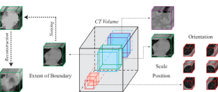
Fig. 1: Spatial properties for effective 3D crop analysis. On the right, one may see the insights brought by crop position, scale, and orientation using spatial anatomical priors. On the left, one may see the importance of boundary delineation.

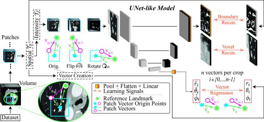
Fig. 2: An overview of our proposed VectorPOSE approach.

To distill relevant spatial information without additional annotation burden, we leverage self-supervised learning (SSL). Recent 3D SSL methods have improved downstream task performances. They generally fall into three types. 1) Contrastive learning [1, 2, 3, 4, 5, 6] stems from metric learning where representations of similar images (e.g., two augmented versions of an image) are encouraged to be close while features of distinct images are contrasted. However, many 3D medical tasks have prohibitively small datasets while requiring cubically more memory, which is incongruous with contrastive methods’ reliance on large datasets, batch sizes, and models [7]. 2) Reconstruction [8, 9, 10, 2, 11] has been shown to outperform supervised transfer learning on 3D data by restoring an original image from a noised or masked version. Still, when analyzing reconstruction results in [9] (see the left side of Fig. 1), one can see significant losses of boundary acuity as well as tissue details. This may suggest an over-focus on local intensity statistics over more robust semantic or spatial understandings of the whole structures. 3) Prediction-based pretext tasks entail solving spatial “puzzles” such as relative position prediction [1], jigsaw unscrambling [1, 12, 13], or scale classification [10]. However, these methods are prone to short-cut learning and over-emphasize discriminative elements (e.g., patch boundaries). Moreover, some approaches propose to learn spatial properties incompletely [10] or indirectly through disparate pretext tasks [9, 14], but implicit learning is suboptimal and uncontrolled. To our best knowledge, no approach adequately covers all key spatial properties important to 3D medical image analysis in practice.

To remedy this gap, we propose a new 3D self-supervised pretraining approach, VectorPOSE (POSE for Position, Orientation, Scale, and Extent), with two novel pretext tasks for learning improved spatial and appearance features. Our first pretext task, Vector Prediction (VP), infers vectors that originate from predefined points within a sampled input crop (e.g., crop center, corners) and terminate at the center of the volume. Vectors encapsulate both magnitude and direction, so predicting multiple vectors with consistent origin points effectively encodes position (with respect to the terminal point), orientation (via vector angles to the terminal point), and scale (where differentials between predicted vector origins represent crop extent). To learn effective local features and address boundary degredations in reconstruction, our second pretext task, Boundary-Focused Reconstruction (BFR), conducts: 1) boundary reconstruction where extracted edges of the patch are explicitly predicted, and 2) voxel reconstruction where original intensity values are predicted with a loss that better preserves boundaries. To demonstrate efficacy, we pretrain and evaluate on three 3D semantic medical image segmentation tasks (i.e., CT cardiac, CT abdominal, MR prostate). VectorPOSE generally outperforms state-of-the-art single- and multi-task methods while exhibiting superior data efficiency compared to known contrastive learning methods.

Our contributions are summarized below.

1. We propose a self-supervised approach, VectorPOSE, that places a holistic emphasis on three key spatial properties (position, orientation, scale) while synergizing learned global information with local, boundary-aware cues.

2. As a cornerstone to spatial understanding, we introduce a novel Vector Prediction (VP) pretext task that succinctly encapsulates key spatial properties and is both effective and extensible. Further, we propose the Boundary-Focused Reconstruction (BFR) pretext task to address pitfalls of recent works and learn improved local features.

3. VectorPOSE is comprehensively evaluated on two 3D CT segmentation datasets (MMWHS [15, 16] & BCV [17]) and one 3D MR prostate dataset [18]. Not only does it outperform recent self-supervised methods in the majority of settings, it also exhibits improved data efficiency without additional training time.

2 Methodology

Before detailing the proposed pretext tasks, we first overview our general pipeline and its major components. Following established self-supervised methods, we pretrain a randomly initialized neural network consisting of an encoder $E$, a decoder $D$, the prediction head $D_{\textit{vp}}$ for Vector Prediction (VP), and the prediction head $D_{\textit{bfr}}$ for Boundary-Focused Reconstruction (BFR). Note that $D_{\textit{vp}}$ employs global information and processes pooled & flattened output features from $E$, while $D_{\textit{bfr}}$ utilizes $D$’s output that has the same resolution as $E$’s input. To pretrain $\{E,D,D_{\textit{vp}},D_{\textit{bfr}}\}$ with VectorPOSE (see Fig. 2), we input patches $x^{i(j)},x^{i(k)},\ldots$ from the $i$th image $X^{i}$ of an unlabeled dataset $\mathcal{D}_{u}$. Stochastic spatial augmentations $\mathcal{T}_{S}$ (e.g., flipping or rotating along each axis) and intensity noising $\mathcal{T}_{I}$ (e.g., local pixel shuffle, masking, intensity shifting) are applied to all input patches independently and in order. The targets for VP & BFR are computed after $\mathcal{T}_{S}$ is applied. After pretraining, $D_{\textit{vp}},D_{\textit{bfr}}$ are discarded while $E,D$ are transferred and fine-tuned on a downstream target task.

2.1 Vector Prediction (VP)

The objective of VP is to distill position, scale, and orientation information from crops by predicting multiple vectors which all point to one standardized location in all dataset volumes (e.g., volume center or center of a chosen object). We refer to this point as the reference landmark, $(x^{i(j)}_{\dashv},y^{i(j)}_{\dashv},z^{i(j)}_{\dashv})$, which denotes the landmark point for crop $x^{i(j)}$ from image $X^{i}$. Reference landmarks across images have anatomical correspondences from which we learn useful priors and structural consistencies. In many 3D tasks, reference landmarks can simply be taken as the center of volumes given rough image alignments. In others, positions of landmarks can be extracted in an unsupervised manner (e.g., center of the left lung as a landmark after lung masks are automatically extracted [19]). To regularize the reference landmark, we randomly jitter coordinates by $\eta$% of each image dimension’s total length.

After image landmarks are obtained, a vector’s origin point concretely defines distance (via its magnitude) and position (via angles) to the reference. For a sampled crop $x^{i(j)}$, we define $n$ vector origin points as $(x^{i(j)}_{0\vdash},y^{i(j)}_{0\vdash},z^{i(j)}_{0\vdash})$, $\ldots$, $(x^{i(j)}_{n-1\vdash},y^{i(j)}_{n-1\vdash},z^{i(j)}_{n-1\vdash})$. In practice, we set these origin points in consistent positions for all crops (e.g., $m$=$0$ at patch center, $m$=$1$ at patch top-right corner, etc.). Mathematically, predicting a single vector is sufficient to describe position and orientation, while two are enough to also cover scale. However, we empirically find that $n$=$9$ vectors (vectors originating from the patch center and 8 corners) improve feature learning (see Section § 3, Tab. 2).

Thus, all vectors belonging to crop $x^{i(j)}$ are defined as $v_{m}^{i(j)}$ ($m=0,\ldots,n-1$) with origin point $(x^{i(j)}_{m\vdash},y^{i(j)}_{m\vdash},z^{i(j)}_{m\vdash})$ and terminal point $(x^{i(j)}_{\dashv},y^{i(j)}_{\dashv},z^{i(j)}_{\dashv})$. The terminal points are identical for all crops from the same image. Below we omit “$i(j)$” for readability. For prediction, we reparameterize vectors into spherical coordinates: let $(x_{m},y_{m},z_{m})=(x_{\dashv}-x_{m\vdash},y_{\dashv}-y_{m\vdash},z_{\dashv}-z_{m\vdash})$; so, $v_{m}=$ ($r_{m}$, $\theta_{m}$, $\rho_{m}$), where $r_{m}=$ $\sqrt{x_{m}^{2}+y_{m}^{2}+z_{m}^{2}}$, $\theta_{m}=\arccos(z_{m}/r_{m})$, and $\phi_{m}=\arctan(y_{m}/x_{m})$ with constraints $r\in[0,\inf)$, $\theta\in[0,\pi]$, and $\phi\in[-\pi,\pi]$. The model regresses the $n$ normalized spherical coordinates of a crop via the VP loss:

$$\mathcal{L}_{\textit{vp}}= \frac{1}{n}\sum_{m=0}^{n-1}\left(||\frac{r_{m}}{R}-\sigma(\hat{r}_{m})||_{1}+||\frac{\theta_{m}}{\pi}-\sigma(\hat{\theta}_{m})||_{1}+\right.$$ (1)

$$\min( ||\frac{\phi_{m}}{\pi}-\tanh(\hat{\phi}_{m})||_{1},||\frac{\phi_{m}+2\pi}{\pi}-\tanh(\hat{\phi}_{m})||_{1},$$

$$||\left.\frac{\phi_{m}-2\pi}{\pi}-\tanh(\hat{\phi}_{m})||_{1})\right)$$

where $\sigma$ is the sigmoid function, $R$ is the radius of a sphere circumscribing the image volume, and $\hat{r}_{m}$, $\hat{\theta}_{m}$, $\hat{\phi}_{m}$ are logits from $E\circ D\circ D_{\textit{vp}}$ (see the bottom right of Fig. 2). To address the $\phi$ angles that are physically close but distant in the parameter space (e.g., $-179\degree$ & +179$\degree$), we take the minimum among targets $\phi_{m},\phi_{m}-2\pi,\phi_{m}+2\pi$ (see Eq. (1)). Also, note that when crops undergo spatial augmentations (e.g., flipping, rotations), the index of each vector’s post-transform origin corresponds with the origin before transforming.

By encapsulating the three key spatial properties into an interdependent task, we prevent training instability and feature interference from independent predictions like when classifications were used [10]. Additionally, vectors represent spatial properties in a continuous space which is a generalized extension of discrete rotation or scale prediction [13].

2.2 Boundary-Focused Reconstruction (BFR)

Complementing the global features from VP, two appearance-focused losses are employed in BFR. To address previous issues of boundary degradation and reduced texture acuity, we first switch the reconstruction criterion from $L_{2}$ loss (as used in [9]) to $L_{1}$ loss, which has been shown to improve both reconstuction quality and boundary accuracy [11]. To further emphasize anatomical delineation, we add an additional boundary reconstruction task where boundaries are extracted via a 3D Scharr edge detector. We select the Scharr transform since it exhibits superior rotational invariance compared to other filters like Sobel. In conjunction with strong augmentations such as texture noising (e.g., local pixel shuffle) and masking (e.g., in-painting or out-painting), explicit edge reconstruction facilitates the learning of general anatomical shapes and boundary extents. The overall BFR loss on a crop is defined as:

$$\mathcal{L}_{\textit{bfr}}=\frac{1}{n}\sum_{m=0}^{n-1}(||{y}_{m}^{v}-\sigma(\hat{y}^{v}_{m})||_{1}+\alpha||y_{m}^{b}-\sigma(\hat{y}^{b}_{m})||_{1}),\vspace{-2.2mm}$$ (2)

where ${y}_{m}^{v}$ and $y_{m}^{b}$ are the targets of the voxel and boundary reconstruction tasks, $\hat{y}^{v}_{m}$ and $\hat{y}^{b}_{m}$ (from $E\circ D\circ D_{\textit{bfr}}$) are the voxel and boundary logits, respectively. $\alpha$ is a scaling term to address the small proportion of boundaries in crops.

2.3 Overall Loss and Implementation

The overall VectorPOSE loss for an image crop is:

$$\mathcal{L}=\lambda\mathcal{L}_{\textit{bfr}}+(1-\lambda)\mathcal{L}_{\textit{vp}}.\vspace{-2mm}$$ (3)

For our UNet-like model, we employ a 3D version of ResNet-50 [20] as the encoder and attach it to a light decoder with bilinear upsampling layers & additions for feature fusion. For $D_{\textit{vp}}$, the lowest encoder output is pooled, flattened, and processed through a 2-layer MLP with 256 hidden dimensions, while $D_{\textit{bfr}}$ uses a single 1x1 convolution. We use $m$=$9$ vectors per patch with a jitter $\eta$=$5$%, and train with $\alpha$=$5$ & $\lambda$=$0.5$.

Method	CT MMWHS					CT BCV					MRI MSD-Prostate
	10%	25%	50%	100%		10%	25%	50%	100%		10%	25%	50%	100%
Random Init.	79.31	87.29	89.15	90.70		30.06	58.48	66.23	75.81		40.05	58.78	69.25	74.24
Models Genesis [9]	80.05	88.14	90.54	91.05		32.03	58.80	66.87	75.79		44.00	60.89	69.55	75.86
SAR [10]	81.48	88.57	90.81	91.14		35.63	60.29	67.52	76.77		42.53	61.02	70.16	74.62
Rubik++ [11]	81.08	88.40	90.94	91.23		33.28	59.83	67.72	76.65		43.70	61.97	71.35	75.81
PGL [21]	79.76	87.50	89.48	90.57		30.99	58.56	66.39	75.98		41.36	59.08	69.97	74.08
MoCo [4]	80.22	87.94	89.60	91.05		31.89	58.95	66.91	76.01		42.07	60.69	70.17	74.31
VectorPOSE (Ours)	83.30	89.43	91.27	91.60		37.88	61.61	68.01	76.53		46.35	63.14	71.22	75.97
p-value	.0335	.0286	.0437	.0564		.0179	.0156	.0388	.0593		.0082	.0098	.0571	.0681

Table 1: Class-averaged Dice score (%) comparisons vs. recent self-supervised 3D medical image segmentation methods. Entries that are bolded & underlined are the best & second-best scores, respectively. p-values are obtained from independent t-tests of the best and second-best scores.

Voxel Rec.	$\mathcal{L}_{1}$	$\mathcal{L}_{1}$	$\mathcal{L}_{1}$	$\mathcal{L}_{1}$	$\mathcal{L}_{1}$	$\mathcal{L}_{1}$
Bound. Rec.		$\mathcal{L}_{1}$	$\mathcal{L}_{1}$	$\mathcal{L}_{1}$	$\mathcal{L}_{1}$	$\mathcal{L}_{1}$
Center Vector			✓	✓	✓	✓
Corner Vector(s)				1	4	8
Dice (%)	80.16	80.80	81.37	82.29	82.75	83.30

Table 2: Ablations on the proposed components on 10% MMWHS. The top two rows contain appearance-based components while the middle two rows have VP settings.

3 Experiments & Results

We implemented all experiments in PyTorch and trained on NVIDIA Tesla P100s (16GB VRAM). For pretraining, volume intensities were normalized between 0 and 1, uninformative regions were excluded, (96, 96, 96) crops were sampled, and augmentations in [9] were applied. We trained using AdamW with a $0.0002$ learning rate & $0.0001$ weight decay for 300 epochs ($\sim$21 hours) with a batch size of 12. For fine-tuning, we normalized volume intensities between 0 and 1, sampled (64, 128, 128) crops, and applied random flipping, brightness, gamma, and blurring. We optimized using AdamW with a learning rate $0.001$ and a weight decay $0.001$ for 200 epochs ($\sim$14 hours) with a batch size of 4 over 8 runs. For evaluation, we used the average Dice-Sørensen Coefficient across foreground classes.

3.1 Datasets

All the datasets are split using a 6:2:2 training:validation:test ratio. Models are pretrained using the full training sets and fine-tuned using 10%, 25%, 50%, or 100% of the training data (if the number of training samples is not divisible, the floor function is applied).

CT MMWHS [16, 15] provides 20 annotated CT volumes segmenting seven cardiac structures (left ventricle, left atrium, right ventricle, right atrium, myocardium, ascending aorta, and pulmonary artery). CT BCV [17] is an abdominal organ segmentation challenge with 30 annotated CT volumes and 13 classes. MRI MSD-Prostate [18] contains 32 labeled MRI (T2, ADC) volumes with two foreground classes.

3.2 Results and Discussion

For fair comparisons, all the methods were pretrained and fine-tuned on the same data splits with the same number of iterations, and allowed an equal budget for hyperparameter tuning. The performances on the three downstream datasets are summarized in Table 1.

From our experimental results, we make the following observations. 1) Our approach generally outperforms recent state-of-the-art multi-task methods and handily beats training from scratch, which supports our hypothesis that more spatially aware models yield more effective representations of 3D crops. More details on the effects of spatially-aware components are discussed in Section § 3.3. 2) The fewer the annotations, the bigger the performance improvements. This is a desirable property for tasks with many biomedical objects with extremely limited labels. Our outperformance over other methods that also use reconstruction [9, 10, 11] shows both the efficacy of our spatial pretext task and superior data efficiency. 3) Both our encoder and decoder are initialized with multi-scale and semantically diverse tasks. Many methods only learn encoder features while suboptimally neglecting decoder parameters (e.g., [21]). Additionally, the decoder receives heterogeneous learning signals from both local-focused BFR and global, spatially-aware VP. This allows for each segment of the model to learn relevant and transferable features and serves as a natural regularizer that prevents overfitting to any single task. In fact, we notice that joint training leads to synergistic improvements. 4) Lesser performance from PGL & MoCo may indicate innate disadvantages in using metric learning techniques with 3D radiology tasks. We hypothesize that this is in part due to the fact that PGL only uses positive samples which inhibits feature learning. The small amount of pretraining images also limits effectiveness. Given that many 3D medical images are highly structured and prior-dependent, we can more effectively learn these priors through spatial prediction tasks that holistically cover multiple key properties.

3.3 Ablations

Here, we explore the contributions of each individual component in our method. Notably, we intend to test our hypothesis about the importance of explicitly learning spatial parameters and compare its efficacy against other proposed methods (e.g., reconstruction). In Table 2, one can see $\sim$0.6% improvement after adding the boundary awareness task, which supports the benefit of explicitly predicting boundaries over voxel reconstruction alone. Next, we see that with increasing $m$ (the number of vectors per crop), performance notably rises. This supports our hypothesis of using spatial awareness as an effective feature-learning principle.

4 Conclusions

We proposed VectorPOSE, a new self-supervised approach for 3D medical image segmentation with two novel pretext tasks: 1) Vector Prediction (VP) to address the lack of spatial understanding (i.e., position, scale, orientation) in existing works; 2) Boundary-Focused Reconstruction (BFR) for improving the understanding of anatomical structure extents through boundary regression. After evaluation on three 3D semantic segmentation datasets, VectorPOSE’s general outperformance over state-of-the-art methods shows that spatial understanding is pertinent for feature learning and may be a promising avenue for future research progress.

5 Compliance with ethical standards

This research was conducted retrospectively using open access human subject data by three publicly available datasets [16, 17, 18]. Ethical approval was not required as confirmed by the licenses attached with the open access datasets.

References

- [1] A. Taleb, W. Loetzsch, N. Danz, J. Severin, T. Gaertner, B. Bergner, and C. Lippert, “3D self-supervised methods for medical imaging,” NIPS, vol. 33, pp. 18158–18172, 2020.
- [2] H. Zheng, J. Han, H. Wang, L. Yang, Z. Zhao, C. Wang, and D. Chen, “Hierarchical self-supervised learning for medical image segmentation based on multi-domain data aggregation,” in MICCAI, 2021.
- [3] D. Zeng, Y. Wu, X. Hu, X. Xu, H. Yuan, M. Huang, J. Zhuang, J. Hu, and Y. Shi, “Positional contrastive learning for volumetric medical image segmentation,” in MICCAI, 2021.
- [4] X. Chen, L. Yao, T. Zhou, J. Dong, and Y. Zhang, “Momentum contrastive learning for few-shot COVID-19 diagnosis from chest CT images,” Pattern Recognition, vol. 113, pp. 107826, 2021.
- [5] K. Chaitanya, E. Erdil, N. Karani, and E. Konukoglu, “Contrastive learning of global and local features for medical image segmentation with limited annotations,” NIPS, vol. 33, 2020.
- [6] H. Zhou, C. Lu, S. Yang, X. Han, and Y. Yu, “Preservational learning improves self-supervised medical image models by reconstructing diverse contexts,” ICCV, pp. 3479–3489, 2021.
- [7] T. Chen, S. Kornblith, M. Norouzi, and G. Hinton, “A simple framework for contrastive learning of visual representations,” in ICML. PMLR, 2020, pp. 1597–1607.
- [8] F. Matzkin, V. F. J. Newcombe, S. Stevenson, A. Khetani, T. Newman, R. Digby, A. Stevens, B. Glocker, and E. Ferrante, “Self-supervised skull reconstruction in brain CT images with decompressive craniectomy,” ArXiv, vol. abs/2007.03817, 2020.
- [9] Z. Zhou, V. Sodha, M. Siddiquee, R. Feng, N. Tajbakhsh, M. Gotway, and J. Liang, “Models genesis: Generic autodidactic models for 3D medical image analysis,” MICCAI, vol. 11767, pp. 384–393, 2019.
- [10] X. Zhang, S. Feng, Y. Zhou, Y. Zhang, and Y. Wang, “SAR: Scale-aware restoration learning for 3D tumor segmentation,” in MICCAI, 2021.
- [11] X. Tao, Y. Li, W. Zhou, K. Ma, and Y. Zheng, “Revisiting Rubik’s cube: Self-supervised learning with volume-wise transformation for 3D medical image segmentation,” in MICCAI. Springer, 2020, pp. 238–248.
- [12] X. Zhuang, Y. Li, Y. Hu, K. Ma, Y. Yang, and Y. Zheng, “Self-supervised feature learning for 3D medical images by playing a Rubik’s cube,” in MICCAI. Springer, 2019, pp. 420–428.
- [13] J. Zhu, Y. Li, Y. Hu, K. Ma, S. Zhou, and Y. Zheng, “Rubik’s Cube+: A self-supervised feature learning framework for 3D medical image analysis,” Medical Image Analysis, vol. 64, pp. 101746, 2020.
- [14] F. Haghighi, M. Taher, Z. Zhou, M. Gotway, and J. Liang, “Transferable visual words: Exploiting the semantics of anatomical patterns for self-supervised learning,” IEEE TMI, vol. 40, pp. 2857–2868, 2021.
- [15] X. Zhuang and J. Shen, “Multi-scale patch and multi-modality atlases for whole heart segmentation of MRI,” Medical Image Analysis, vol. 31, pp. 77–87, 2016.
- [16] X. Zhuang, “Challenges and methodologies of fully automatic whole heart segmentation: A review,” Journal of Healthcare Engineering, vol. 4, pp. 371–407, 2013.
- [17] “Multi-atlas labeling beyond the cranial vault - workshop and challenge,” 2015, Accessed January 2021 at https://www.synapse.org/#!Synapse:syn3193805/wiki/89480.
- [18] A. L. Simpson, M. Antonelli, S. Bakas, M. Bilello, K. Farahani, B. Ginneken, A. Kopp-Schneider, B. A. Landman, G. J. S. Litjens, B. H. Menze, O. Ronneberger, R. M. Summers, P. Bilic, P. F. Christ, R. K. G. Do, M. J. Gollub, J. Golia-Pernicka, S. Heckers, W. R. Jarnagin, M. McHugo, S. Napel, E. Vorontsov, L. Maier-Hein, and M. J. Cardoso, “A large annotated medical image dataset for the development and evaluation of segmentation algorithms,” ArXiv, vol. abs/1902.09063, 2019.
- [19] B. Zhao, G. Gamsu, M. S. Ginsberg, L. Jiang, and L. H. Schwartz, “Automatic detection of small lung nodules on CT utilizing a local density maximum algorithm,” Journal of Applied Clinical Medical Physics, vol. 4, no. 3, pp. 248–260, 2003.
- [20] K. He, X. Zhang, S. Ren, and J. Sun, “Deep residual learning for image recognition,” CVPR, pp. 770–778, 2016.
- [21] Y. Xie, J. Zhang, Z. Liao, Y. Xia, and C. Shen, “PGL: Prior-guided local self-supervised learning for 3D medical image segmentation,” ArXiv abs/2011.12640, 2020.