Topological transitions of the generalized Pancharatnam-Berry phase

Abstract

Distinct from the dynamical phase, in a cyclic evolution, a system’s state may acquire an additional component, a.k.a. geometric phase. The latter is a manifestation of a closed path in state space. Geometric phases underlie various physical phenomena, notably the emergence of topological invariants of many-body states. Recently it has been demonstrated that geometric phases can be induced by a sequence of generalized measurements implemented on a single qubit. Furthermore, it has been predicted that such geometric phases may exhibit a topological transition as function of the measurement strength. Here, we demonstrate and study this transition experimentally employing an optical platform. We show the robustness to certain generalizations of the original protocol, as well as to certain types of imperfections. Our protocol can be interpreted in terms of environment-induced geometric phases.

I Introduction

When a quantum state undergoes a cyclic evolution, the phase acquired is given by the well-known dynamical component plus an additional contribution, associated with the geometrical features of the path followed by the state. This additional contribution is known as the geometric phase. The general framework for the emergence of a geometric phase has been pointed out first by Berry [1] in the context of adiabatic quantum evolution. A specific realization of this phase had been earlier considered by Pancharatnam [2] in his study of generalized interference theory. Pancharantnam’s theory shows how geometric phases can be acquired in a non-adiabatic cyclic evolution, noting that these are given by the area enclosed by the respective trajectory of the system in the state space. The Pancharantnam phase can be observed following a sequence of running projective measurements, each of a different observable, where the last measurement projects on the initial state [3, 4]. Geometric phases have found applications in several fields of physics [5], in particular, in optics [6, 7, 8, 9] and condensed matter physics [10, 11, 12, 13, 14]. Importantly, the Berry phase is a key theme for understanding topological phases of matter [14]. For instance, the Berry phase plays the role of a topological invariant in one-dimensional chiral symmetric systems [15, 16] and serve as the fundamental building block in the definition of other topological invariants, such as Chern numbers [17]. Going beyond Hamiltonian dynamics, the emergence of geometric phases has been predicted and observed in the context of non-Hermitian evolution [18, 19, 20]; such phases were further shown to emerge following a sequence of weak measurements [21, 22]. Further pursuing the latter theme, a major theoretical development has revealed that dynamics comprising multiple measurements may assign topological features to geometric phases. In particular, the limits of weak and strong measurement are topologically distinct [22, 23, 24]. This prediction has recently been confirmed employing a superconducting qubit platform [25]. That study has implemented postselection on each individual measurement. This aligns with the original theoretical proposal [22, 23, 24], yet it leaves the question open: to what extent is the predicted topological transition a feature of the specific laid-down protocol?

The experiment reported here not only employs a platform different from that of Ref. [25] (namely, an optical platform), but also introduces a protocol which is conceptually different: rather than exercising postselection on each individual detector’s readout, here we implement postselection on a joint readout of all measurements of the run. We find that a topological phase transition takes place also under such generalized conditions, with distinct values of the topological number characterizing the respective limits of projective and infinitely weak measurements. Our experimental procedure consists of a sequence of measurements, each implemented by a set of optical elements. The key optical element is a polarization-sensitive beam displacer, which is used to execute a weak measurement on the polarization state of a laser beam. Employing additional elements (quarter wave plates, compensating wave plates) serves to tune the measurement to a specific observable. The strength of the measurement is determined by the ratio of the beam width and the difference of transverse displacements of orthogonal polarizations. Importantly, the detector’s readout is, in fact, the polarisation degree of freedom of the photon, which, in turn, could be viewed as the system, while the transverse position can be viewed as the environment. Our protocol could then be interpreted as an environment inducing a geometric phase, highlighting the dual nature of detector/environment. Finally, we investigate the robustness of the observed topological properties with respect to setup imperfections.

II Results

Theoretical overview. We consider a class of processes where $N$ measurements are performed on a quantum system, as shown in Fig. 1a. Each step is a post-selected measurement associated with the polarization state $\left|\theta,\phi\right\rangle$, where $\theta$ and $\phi$ stand for the polar and azimuthal coordinates on the Bloch sphere, respectively. We can define a sequence of measurements $(\theta,\phi_{n})$ for a fixed value of $\theta\in[0,\pi]$ while the azimuth is spanned in discrete steps $\phi_{n}=2\pi n/(N+1)$. Let us denote the acquired geometric phase $\chi_{\eta}(\theta)$, where $\eta\in[0,\infty)$ is introduced to indicate the strength of the measurement. It can be shown that $\Delta\chi_{\eta}=\chi_{\eta}(\pi)-\chi_{\eta}(0)=2\pi m$, where $m$ is an integer – see Supplementary Information (SI),  Section 1.3, for more details.

As illustrated in Fig. 1b, for infinitely weak measurements, $\eta\rightarrow 0$, the effect of each measurement is vanishingly small. Therefore, $\chi(\theta)=0$ for any value of $\theta$, implying that $\Delta\chi_{\eta\rightarrow 0}=0$. However, in the limit of projective measurements, strong measurement, one observes that $\Delta\chi_{\eta\rightarrow\infty}=2\pi$, as shown in Pancharatnam’s geometric-phase theory [2]. An example of the latter case, strong measurement limit, is illustrated in Fig. 1c: When $\theta=0$, the measurement sequence does not change the projected state. Thus, the trajectory on the Bloch sphere shrinks to a single point independently of the measurement strength. In consequence, the enclosed area – and the geometrical phase – is zero. For $\theta\rightarrow 0$ , the state follows a loop close to the initial projected state, acquiring a small geometric phase. As $\theta\rightarrow\pi$, the state follows a similar loop close to the south pole of the Bloch sphere, thus the enclosed geometric phase is close to $2\pi$. This gives $\Delta\chi_{\eta\rightarrow\infty}=2\pi$, as stated above. The distinction between $\Delta\chi_{\eta\rightarrow 0}=0$ and $\Delta\chi_{\eta\rightarrow\infty}=2\pi$ suggests the existence of a transition in the behavior of the geometric phase, as the measurement strength $\eta$ is varied. Since $\Delta\chi=2\pi m$, the nature of the transition is topological.

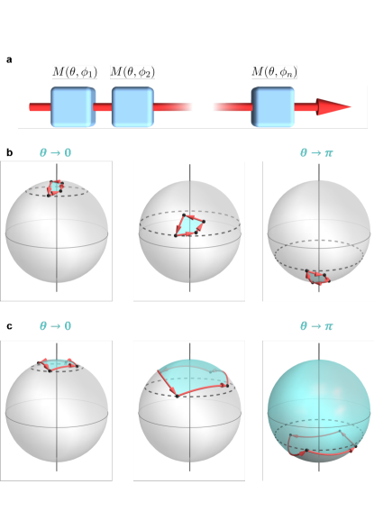
Figure 1: Measurement-induced phase and its topological transition. a. The state trajectory of a system is determined by a series of $N$ measurements along different directions $(\theta,\phi)$. b and c. The state trajectory on the Bloch sphere for a sequence of three measurements with strength $\eta=0.2$ (b) and $\eta=0.7$ (c) for different values of $\theta$. The black dashed line corresponds to $\theta$, at which the measurements are performed. The black points connected by red arrows denote the system state trajectory, as induced by the measurements. The colored portion of the Bloch sphere is the solid angle subtended by the respective trajectory.

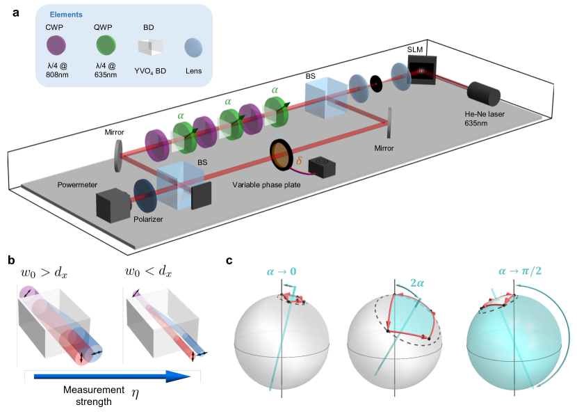
Figure 2: Optical implementation of a sequence of weak polarization measurements. a. Experimental setup used to detect the geometrical phase acquired due to a sequence of polarization measurements. A 632.9 nm laser emits a vertically polarized Gaussian beam which impinges on a spatial light modulator (SLM) to obtain a beam with a certain width $w_{0}$. The beam is split into two paths: in one is subjected to a sequence of transformations, while a spatially uniform phase $\delta$ is applied to the other path. Each stage is composed of a quarter-wave plate (QWP), whose fast axis is oriented at angle $\alpha$ with respect to the vertical, a beam displacer (BD), and a QWP for 808 nm acting as the compensation wave plate (CWP). Finally, the output power of the interference is recorded after the recombined beam passes through a vertical polarizer. b. The measurement strength $\eta=d_{x}/w_{0}$ is controlled by varying the waist parameter $w_{0}$ of the input beam. When $w_{0}$ is much larger than the beam displacement $d_{x}$, the displacement is ineffectual, corresponding to a weak measurement. For $w_{0}<d_{x}$, the two polarizations become two well-separated beams, leading to a projective measurement in the limit $w_{0}\rightarrow 0$. c. In contrast to the examples exhibited in Fig. 1b-c, the sequence of measurements produced by this setup corresponds to a circle of $\theta=2\alpha$, which is additionally rotated by $2\alpha$ around the x axis of the Bloch sphere. This does not affect the subtended area and, consequently, the accumulated geometric phase.

Experimental setup. We demonstrate the existence of this topological transition in an optical experiment where the qubit state is associated with the polarization of a coherent beam. As illustrated in Fig. 2a, the beam goes through a series of $N=3$ identical optical stages which emulate the measurement steps. Each stage is composed of a quarter-wave plate (QWP), whose fast axis is oriented at angle $\alpha=\theta/2$ with respect to the vertical, followed by a YVO₄ beam displacer (BD) and an additional compensating wave plate (CWP). The BD’s ordinary and extraordinary axes are aligned along $\mathbf{\hat{y}}$ and $\mathbf{\hat{x}}$, respectively. Therefore, the BD shifts the centroid of the horizontally polarized component by a distance $d_{x}$, keeping the vertically polarized contribution unchanged. The BD essentially performs a measurement in the vertical/horizontal polarization basis, as the horizontally polarized component of the beam is spatially displaced. If the beam waist $w_{0}$ is larger than $d_{x}$, the measurement is weak, since there is no sharp separation between the two polarizations components (see Fig. 2b). If the waist is much smaller than the displacement, $w_{0}\ll d_{x}$, this implements a projective measurement, as the two polarization components are completely separated. Therefore, we can control the measurement strength by modifying $w_{0}$. The CWP with a vertically aligned fast axis is used to compensate for the phase difference between the two polarization components accumulated while propagating inside the BD.

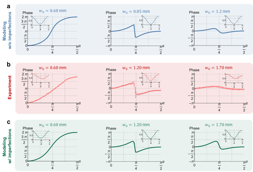
Figure 3: Experimentally measured and theoretically simulated geometric phase. Topological transition in the measurement-induced geometric phase $\chi(\alpha=\theta/2)$: a. theoretical modeling, b. experimental results, c. modeling incorporating the imperfection of the birefringent crystals. The left column corresponds to a narrow beam (small $w_{0}$, strong measurement) and features $\Delta\chi=2\pi$. The right column corresponds to a large beam width (weak measurement) and exhibits $\Delta\chi=0$. The middle column represents a point close to the transition: the phase $\chi(\alpha)$ exhibits a sharp change near $\alpha=\pi/4$, and the interference contrast vanishes near $\alpha=\pi/4$, enabling the change of the phase’s topological behavior.

The role of the QWPs is to implement the desired sequence of measurement directions $(\theta,\phi_{n})$ on the Bloch sphere. The rotation by angle $\alpha$ enables controlling the polar angle $\theta$ of the measurement axis. The sequence of measurements induced by the setup in Fig. 2a corresponds to the directions $(\theta,\phi_{n})$ rotated by an angle $\theta=2\alpha$ around the y axis of the Bloch sphere, cf. Fig. 2c. The details of this correspondence are explained in the Section 2.1. Given the geometric nature of the induced phase, the expected topological transition remains unaffected by this rotation, both qualitatively and quantitatively. Finally, to complete the cyclic evolution, the polarization state is projected onto the initial state using a polarizer.

Our aim is to investigate the geometrical phase acquired by the non-deflected beam (corresponding to the measurement postselected to yield a null outcome). This is done by interfering the final state with the reference beam, which only experiences a controllable phase shift $\delta$ introduced by a variable phase plate. The output power at the interferometer exit is recorded as a function of $\delta$. The shift of this curve corresponds to the acquired geometric phase. The input beam is generated by means of a spatial light modulator (SLM) that displays a hologram allowing to tailor the beam waist through the technique introduced in Ref. [26]. We set the input beam’s polarization state to be vertical ($\mathbf{\hat{y}}$), corresponding to the initial state in the direction $(\theta,\phi_{0})$ in the theoretical protocol. Based on this setup, the measurement protocol to unveil the hidden topological transition is given as follows. The strength of our intermediate $N=3$ measurements is regulated by varying the waist parameter of the input beam: the value of $w_{0}$ is inversely proportional to the measurement strength $\eta=d_{x}/w_{0}$ (see Fig. 2c). For a fixed waist parameter, we proceed to get power readouts as a function of the reference arm phase shift $\delta\in[0,2\pi]$, while $\alpha=\theta/2$ is kept constant. From here, it is possible to retrieve the accumulated geometrical phase $\chi_{\eta}(\theta=2\alpha)$ for a given orientation of QWPs, $\alpha$, by proper curve fitting. By varying the QWPs orientation, it is possible to reconstruct the behavior of $\chi_{\eta}(\theta=2\alpha)$ for all $\alpha$ for a given measurement strength.

Experimental results. Here, we discuss the experimental results and their relation to the theoretical predictions. Since the postselection in our experiment goes beyond the original theoretical proposal, we have modeled the experiment to confirm the presence of a topological transition theoretically (see Section 2 of SI). Figure 3a shows that when $w_{0}$ is sufficiently small, i.e. strong measurement regime, the simulation predicts $\Delta\chi=\chi(\alpha=\pi/2)-\chi(\alpha=0)=2\pi$, while for the case of weak measurements ($w_{0}<d_{x}$), $\Delta\chi=0$. A sharp transition is occurs at $w_{0}=0.85$ mm, where the interference contrast vanishes for $\alpha\approx\pi/4$, enabling the abrupt change of the phase behavior. The experiment was carried on by performing measurements for $w_{0}$ between 0.6 mm and 2.5 mm. The experimental results, shown in Fig. 3b, clearly exhibit a similar transition between $\Delta\chi=2\pi$ for small $w_{0}$ and $\Delta\chi=0$ for large $w_{0}$, as well as the vanishing contrast at the transition.

The difference $\Delta\chi=\chi(\pi/2)-\chi(0)$ in the observations is not strictly equal to $0$ or $2\pi$, but can slightly deviate from these values. This is seen most prominently for $w_{0}=0.6$ mm. We attribute this to the stability of the Mach-Zehnder interferometer, in particular to a small drift in the phase between the two arms during the measurement process (which was performed in 45 minutes). We emphasize that this does not violate the topological quantization of $\Delta\chi$, but introduces an error in its extraction. In all the cases, the extracted $\Delta\chi$ is close to either $0$ or $2\pi$, making the determination of the topological index $m$ straightforward. The vanishing contrast at the transition also confirms the expected phenomenology of the topological transition.

We note that the waist $w_{0}^{*}$ at which the transition happens clearly deviates from the theory predictions: $w_{0}^{*}=0.85$ mm in the simulation, while $w_{0}^{*}=1.2$ mm in the experiment. We attribute this deviation to the fact that the surfaces of the BDs are parallel within a few tens of arcseconds, as stated by the manufacturer and verified by us independently. This tiny angle between the two surfaces induces a small transverse wavevector difference between the two components. We have incorporated this effect into our theoretical modeling, the results of which are presented in Fig. 3c. With this, we are able to reproduce the change in the transition location. A detailed analysis of these imperfections and the enhanced modeling can be found in Section 2.2 of the SI.

Theoretical studies have predicted [23, 24] that the topological transition only exists if the dynamical phases are compensated accurately enough. In our work, this condition is satisfied. In Fig. 4 we explored theoretically the topological phase diagram considering the additional parameter $\gamma$ corresponding to the optical retardation of the CWP. The results show that there is a range of values of $\gamma$ where the topological transition can be observed, both in the ideal scenario and in the case of imperfect optical elements.

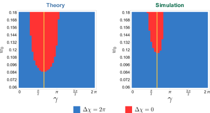
Figure 4: Topological phase dependence on compensating waveplates. The phase diagram (theoretical) depicting the topological properties of the measurement-induced phase as a function of beam waist $w_{0}$ and the compensation phase $\gamma$. We present the results of a theory simulation without (left) and including (right) the experimental imperfections of the birefringent crystals. Note that the trivial phase with ($\Delta\chi=0$) exists only in a narrow interval of the phase compensation parameter The vertical line indicates the parameters used in our experiment. The imperfections of birefringent crystals clearly make the trivial region shrink, yet do not eliminate the topological transition.

III Discussion

We have demonstrated that measurement-induced geometric phases in optical systems exhibit a topological transition. In particular, we consider a family of processes parameterized by a variable $\alpha$ and a measurement strength $\eta$. We demonstrated that the geometrical phase, with respect to $\eta$ and $\alpha$, exhibits a nontrivial topology. More precisely, the variation $\Delta\chi$ in geometrical phase as a function of $\alpha$ undergoes a sharp transition of $2\pi$ as $\eta$ is varied. The parameter $\eta$ can be viewed as the coupling strength with an environment, here represented by the light’s spatial degree of freedom. In this framework, our observations can be interpreted as topological transitions induced by the coupling to an external environment. The topological transition is robust to amending the protocol and the imperfections in the measurement process. The location of the topological transition depends on specific details of the system (quality of beam displacers, retardation of the compensating waveplates, etc.). This sensitivity of the transition location may be useful for characterizing optical elements or for sensing. We leave this, however, to future investigations.

Supplementary Information accompanies this manuscript.

Acknowledgments This work was supported by Canada Research Chairs (CRC), Canada First Research Excellence Fund (CFREF) Program, NRC-uOttawa Joint Centre for Extreme Quantum Photonics (JCEP) via High Throughput and Secure Networks Challenge Program at the National Research Council of Canada, Deutsche Forschungsgemeinschaft (German Research Foundation) through Project No. 277101999, TRR 183 (Project C01), and Projects No. EG 96/13-1, GO 1405/6-1, and MI 658/10-2, Helmholtz International Fellow Award, the Israeli Science Foundation (ISF), NSF Grant No. DMR-2037654, and the U.S.–Israel Binational Science Foundation (BSF).

Author Contributions K.S., A.R., Y.G., and E.K. conceived the idea; M.F., A.D., K.S., and E.K. designed the experiment; M.F. and K.S. performed the theoretical simulations; M.F. and A.D. performed the experiment and collected the data; M.F., A.D., and K.S. analysed the data; M.F., K.S., A.D., and A.R. prepared the first version of the manuscript. All authors discussed the results and contributed to the text of the manuscript.

Author Information The authors declare no competing financial interests. Correspondence and requests for materials should be addressed to aderrico@uottawa.ca.

Supplementary Information for:
Topological transitions of the generalized Pancharatnam-Berry phase

Section 1 Theoretical protocol and its relation to the experimental setup

Here we provide a brief theoretical background on quantum measurement theory, on measurement induced geometric phases, and the topological transition in them, as well as connect the quantum measurement formalism to the optical setup employed in the paper.

Section 1.1 Null-weak measurements of different observables in the polarization space

The formalism applies to the transition reported in the main text when regarding the polarization of the laser beam as a quantum polarization state $\left|\theta,\phi\right\rangle=\cos(\theta/2)\left|\uparrow\right\rangle+e^{i\phi}\sin(\theta/2)\left|\downarrow\right\rangle$ of a photon, where $\left|\uparrow\right\rangle$ and $\left|\downarrow\right\rangle$ label the linearly independent vertical and horizontal polarizations respectively with $\theta\in[0,\pi]$ and $\phi\in[0,2\pi)$.

In the most general setting, a measurement of a quantum system in a state $\left|\psi\right\rangle$ returns an outcome $r$ with probability $P(r)=\langle\psi|M_{r}^{\dagger}M_{r}|\psi\rangle$, while the state is updated as $\left|\psi\right\rangle\to\left|\psi^{\prime}\right\rangle=M_{r}\left|\psi\right\rangle/\sqrt{P(r)}$. The process is controlled by the Kraus operators $M_{r}$, which depend on the specific detection process and fulfil $\sum_{r}M_{r}^{\dagger}M_{r}=1$ due to overall probability conservation [27]. For what we are concerned here, we specialize in a measurement process, known as null weak measurement, with two possible outcomes, $r=+,\,-$, and corresponding Kraus operators

$$M_{+}=\sqrt{\zeta}\left|\downarrow\right\rangle\left\langle\downarrow\right|,\quad M_{-}=\left|\uparrow\right\rangle\left\langle\uparrow\right|+\sqrt{1-\zeta}\left|\downarrow\right\rangle\left\langle\downarrow\right|,$$ (S1)

where $0\leq\zeta\leq 1$ corresponds to the measurement strength $\eta=\sqrt{-\ln\left(1-\zeta\right)}$. For $\zeta=1$ ($\eta\rightarrow\infty$), the measurement is projective: the operation projects the state on $\left|\downarrow\right\rangle$ if $r=+$ and $\left|\uparrow\right\rangle$ if $r=-$. For $\zeta<1$, however, we either have a collapse to $\left|\downarrow\right\rangle$ (“click”, described by $M_{+}$) or no collapse (“no-click” or “null measurement”, described by $M_{-}$). In the latter case, the system’s state is updated to a the post-measurement state, which depends on the pre-measurement one.

The measurement procedure in Eq. (S1) corresponds to an imperfect, or weak, measurement of $\sigma_{z}$. This can be generalized to measure arbitrary observables, i.e. to distinguish two arbitrary basis states. A direction $\mathbf{n}=(\sin\theta\cos\phi,\sin\theta\sin\phi,\cos\theta)$ is identified by the polar and azimuthal angles $\theta$ and $\phi$ on the Bloch sphere. The corresponding orthogonal basis states, $\left|\uparrow_{\mathbf{n}}\right\rangle$ and $\left|\downarrow_{\mathbf{n}}\right\rangle$, are defined as eigenstates of $\mathbf{n}\cdot\bm{\sigma}$ associated with the respective eigenvalue $\pm 1$. For $\phi=0$ and $\pi$ these states correspond to two mutually orthogonal linear polarizations, whereas for all other values of $\phi$ they correspond to general elliptic polarizations. The analog of Eq. (S1) is then given by $M_{+}\left(\mathbf{n}\right)=\sqrt{\zeta}\left|\downarrow_{\mathbf{n}}\right\rangle\left\langle\downarrow_{\mathbf{n}}\right|$, $M_{-}\left(\mathbf{n}\right)=\left|\uparrow_{\mathbf{n}}\right\rangle\left\langle\uparrow_{\mathbf{n}}\right|+\sqrt{1-\zeta}\left|\downarrow_{\mathbf{n}}\right\rangle\left\langle\downarrow_{\mathbf{n}}\right|$.

Section 1.2 Measurement-induced geometric phases

In order to induce a geometric phase, one needs to use multiple measurements. We label them by $j=1,...,N$. Each measurement is determined by the observable it measures, i.e., by the direction $\mathbf{n}_{j}$. The respective Kraus operators are $M_{r_{j}}^{(j)}=M_{r_{j}}\left(\mathbf{n}_{j}\right)$, where $r_{j}=\pm$ is the readout of measurement $j$.

For each such measurement with a given outcome, the phase of the post-measurement state is gauge-dependent, hence non-physical. However, if a sequence of measurements leads to a post-measurement final state $\left|\psi_{f}\right\rangle$ which is proportional to the initial one, $\left|\psi_{0}\right\rangle$, the phase difference between $\left|\psi_{f}\right\rangle$ and $\left|\psi_{0}\right\rangle$ is a legit observable given by

$$\chi_{\{r_{j}\}}={\rm arg}\langle\psi_{0}|\psi_{f}\rangle={\rm arg}\left\langle\psi_{0}\right|M_{r_{N}}^{(N)}\dots M_{r_{2}}^{(2)}M_{r_{1}}^{(1)}\left|\psi_{0}\right\rangle,$$ (S2)

where $r_{j}$ is the outcome (readout) of the $j$-th measurement, whose effect is encoded in the Kraus operator $M_{r_{j}}^{(j)}$.

Note that even if the final state, $\left|\psi_{f}\right\rangle$, differs from the initial one, the phase defined in Eq. (S2) is still well-defined: this can be understood introducing a fake projective measurement onto the initial state, $\left|\psi_{0}\right\rangle\left\langle\psi_{0}\right|$, after the application of all $M_{r_{j}}^{(j)}$, in order to force $\left|\psi_{f}\right\rangle\propto\left|\psi_{0}\right\rangle$. Therefore, Eq. (S2) defines a legitimate observable for a general sequence of measurements. The sequence of (normalized) post-measurement intermediate states, $\left|\psi_{0}\right\rangle$, $M_{r_{1}}^{(1)}\left|\psi_{0}\right\rangle$, $\dots$, $M_{r_{N}}^{(N)}...M_{r_{1}}^{(1)}\left|\psi_{0}\right\rangle$, defines a trajectory on the Bloch sphere. This trajectory is given by the set of geodesics connecting the states. For Hermitian Kraus operators, $M_{r_{j}}^{(j)\dagger}=M_{r_{j}}^{(j)}$ (which is the case in Eq. (S1)), the measurement-induced phase, (S2), has a geometric interpretation as $\chi_{\{r_{j}\}}=\Omega/2$, where $\Omega$ is the solid angle subtended by the trajectory on the Bloch sphere [21, 22, 23, 24].

Section 1.3 Protocol for topological transition in measurement-induced phases

Consider a family of measurement sequences, defined in the main text. Each sequence consists of $N$ measurements corresponding to $\left(\theta,\phi_{j}=2\pi j/(N+1)\right)$, where $j=1,...,N$ is the measurement number. The family is obtained when considering such sequences at all $\theta\in[0,\pi]$. We perform postselection, which restricts measurement readouts to be $r_{j}=-$ for all $j$. According to Eq. (S2), this defines a phase $\chi_{\left\{-\right\}}(\theta)$ for each measurement sequence in the family. For briefness, we denote this phase $\chi(\theta)$.

The function $\chi(\theta)$ possesses a topological invariant. This follows from the fact that at $\theta=0$ and $\theta=\pi$, $M_{r_{j}}^{(j)}\left|\psi_{0}\right\rangle=\left|\psi_{0}\right\rangle$ for all $j$, implying that $\left|\psi_{f}\right\rangle=\left|\psi_{0}\right\rangle$. That is, the measurements do not change the system state, so that the resulting phase is trivial: $e^{i\chi(0)}=e^{i\chi(\pi)}=1$. As any phase, the measurement-induced phase is defined up to an integer multiple of $2\pi$. Without loss of generality, we can set $\chi(0)=0$. This, however, eliminates the freedom of adding multiples of $2\pi$ at all other $\theta$ due to the natural demand of continuity of $\chi(\theta)$. In particular, $\chi(\pi)$ may be non-zero; yet $e^{i\chi(\pi)}=1$ implies that $\chi(\pi)=2\pi m$ with integer $m$. In other words, the difference $\Delta\chi=\chi(\pi)-\chi(0)$, must be quantized in units of $2\pi$, as stated in the main text. Further, the quantization of $\Delta\chi$ implies that its value cannot be changed by continuous deformations of the function $\chi(\theta)$. Therefore, $\Delta\chi$ constitutes a topological invariant.

As discussed in the main text, for infinitely weak ($\zeta\to 0$) and projective ($\zeta\to 1$) measurements $\Delta\chi_{\zeta\rightarrow 0}=0$ and $\Delta\chi_{\zeta\rightarrow 1}=2\pi$ respectively. This necessitates a jump in the topological invariant, i.e., a topological transition, at some critical measurement strength, $\zeta_{c}\in[0,1]$.

Section 1.4 Detection of measurement-induced geometric phases

In order to detect a measurement-induced phase, one needs to interfere the state that underwent measurements with the initial unmeasured state, as in Fig. 2a. Here we provide a theoretical description of this in the quantum measurement formalism.

The incoming photon in polarization state $\left|\psi_{0}\right\rangle$ becomes, after the beam splitter, the state $\left|\psi\right\rangle=\frac{1}{\sqrt{2}}\left|\psi_{0}\right\rangle\otimes\left(\left|0\right\rangle+\left|1\right\rangle\right)$ where $\left|0\right\rangle$ and $\left|1\right\rangle$ refer to the two arms of the interferometer. A sequence of measurements with Kraus operators $M_{r_{j}}\left(\mathbf{n}_{j}\right)$ is performed in the interferometer arm denoted as $\left|0\right\rangle$. The arm denoted as $\left|1\right\rangle$ features only a phase shifter, $\delta$. Therefore, after passing through the respective interferometer arms the photon state is

$$\left|\psi\right\rangle_{int}=\frac{1}{\sqrt{2}}\left[\sum_{\{r_{j}\}}\left|\Psi_{0}\left(\{r_{j}\}\right)\right\rangle\otimes\left|0\right\rangle+\left|\Psi_{1}\right\rangle\otimes\left|1\right\rangle\right],$$ (S3)

where

$$\left|\Psi_{0}\left(\{r_{j}\}\right)\right\rangle =M_{r_{N}}^{(N)}...M_{r_{1}}^{(1)}\left|\psi_{0}\right\rangle\otimes\left|\left\{r_{j}\right\}\right\rangle,$$ (S4)

$$\left|\Psi_{1}\right\rangle =e^{i\delta}\left|\psi_{0}\right\rangle\otimes\left|\left\{r_{j}=-\right\}\right\rangle.$$ (S5)

Here we introduced the collective state of all the detectors, $\left|\left\{r_{j}\right\}\right\rangle$. In the arm denoted by $\left|1\right\rangle$ the detectors do not interact with the photon and thus stay in the no-click position.

The second beam splitter converts $\left|0\right\rangle\rightarrow\frac{1}{\sqrt{2}}\left(\left|0\right\rangle+\left|1\right\rangle\right)$, $\left|1\right\rangle\rightarrow\frac{1}{\sqrt{2}}\left(\left|0\right\rangle-\left|1\right\rangle\right)$, so that the output state is

$$\left|\psi\right\rangle_{out}=\frac{1}{2}\biggl{[}\left(\left|\Psi_{1}\right\rangle+\sum_{\{r_{j}\}}\left|\Psi_{0}\left(\{r_{j}\}\right)\right\rangle\right)\otimes\left|0\right\rangle+\left(-\left|\Psi_{1}\right\rangle+\sum_{\{r_{j}\}}\left|\Psi_{0}\left(\{r_{j}\}\right)\right\rangle\right)\otimes\left|1\right\rangle\biggr{]}.$$ (S6)

Therefore, the probability of the photon appearing at output ports $\left|0\right\rangle$ or $\left|1\right\rangle$ is given by

$$P_{0/1} =\frac{1}{2}\left[1\pm\sum_{\{r_{j}\}}\mathrm{Re}\thinspace e^{-i\delta}\langle\Psi_{1}|\Psi_{0}\left(\{r_{j}\}\right)\rangle\right]$$

$$=\frac{1}{2}\left[1\pm\mathrm{Re}\thinspace e^{-i\delta}\left\langle\psi_{0}\right|M_{-}^{(N)}...M_{-}^{(1)}\left|\psi_{0}\right\rangle\right].$$ (S7)

Note that only the term with no-click readouts, $\{r_{j}=-\}$, in the measured interferometer arm contributes to the interference, which thus enables the observation of the measurement-induced phase, cf. Eq. (S2) and Section 1.2. In other words, the interference implicitly performs the postselection to $\{r_{j}=-\}$ required by the definition of $\chi(\theta)$, cf. Section 1.3.

Section 2 Optical implementation of the null-weak measurement

In our optical implementation of the measurements, the detectors are not two-state systems with possible readouts $r=\pm$. We use the photon spatial degree of freedom, i.e., its location in the $xy$ plane (transverse to the propagation direction). The formal description of this is as follows. The incident photon’s electric field can be described as

$$\mathbf{E}_{0}(x,y)=\left(\begin{array}[]{c}E_{0y}(x,y)\\ E_{0x}(x,y)\end{array}\right)=\left(\begin{array}[]{c}E_{0y}\\ E_{0x}\end{array}\right)\sqrt{\frac{2}{\pi w_{0}^{2}}}e^{-(x^{2}+y^{2})/w_{0}^{2}}e^{ikz}.$$ (S12)

The measurement is implemented via a beam displacer (see Figure S1a) that shifts the $x$-polarized component in space:

$$\mathbf{E}(x,y)=\mathrm{BD}\>\mathbf{E}_{0}(x,y)=\sqrt{\frac{2}{\pi w_{0}^{2}}}\left(\begin{array}[]{c}e^{ikn_{y}L_{y}}E_{0y}e^{-(x^{2}+y^{2})/w_{0}^{2}}\\ e^{ikn_{x}L_{x}}E_{0x}e^{-(\left[x-d_{x}\right]^{2}+y^{2})/w_{0}^{2}}\end{array}\right)e^{ikz}.$$ (S15)

Apart from the displacement, the phases associated with propagation in the beam displacer, $kn_{x}L_{x}$ and $kn_{y}L_{y}$, are imprinted onto the polarization components. The overall phase is not important, whereas the difference $\gamma=kn_{x}L_{x}-kn_{y}L_{y}$ may lead to observable consequences, cf. Fig. 4. In our protocol we compensate this phase difference, see below. Therefore, here we put, for simplicity, $kn_{x}L_{x}=kn_{y}L_{y}=0$.

If, after experiencing the BD, the beam were to interfere with the original beam, the interference term would be

$$\int dx\,dy\>\mathbf{E}_{0}^{*}(x,y)\mathbf{E}(x,y)=\left|E_{0y}\right|^{2}+\left|E_{0x}\right|^{2}e^{-d^{2}/(2w_{0}^{2})}=\left(\begin{array}[]{c}E_{0y}\\ E_{0x}\end{array}\right)^{\dagger}M_{-}\left(\begin{array}[]{c}E_{0y}\\ E_{0x}\end{array}\right),$$ (S20)

where $M_{-}$ is the matrix defined in Eq. (S1) if $\left|\uparrow\right\rangle$ is interpreted as the $y$ polarization and $\left|\downarrow\right\rangle$ as the $x$ polarization, while $\sqrt{1-\zeta}=e^{-d_{x}^{2}/(2w_{0}^{2})}$. Therefore, a beam displacer implements a postselected null weak measurement in the photon’s polarization space. The measurement strength $\eta=\sqrt{-\ln\left(1-\zeta\right)}=d_{x}/w_{0}$, as defined in the main text. The limit of projective measurement corresponds to $\eta\rightarrow\infty$, while the infinitely weak measurement corresponds to $\eta\rightarrow 0$.

Note that in our actual setup, cf. Fig. 2a, the interference happens after three beam displacements have been performed. Therefore, the postselection is implemented not on the readout of each individual measurement, but on the combined “readout” of all measurements. This consitutes an important conceptual difference compared to the original definition of the measurement-induced phase and its topological transition, cf. Section 1.2 and Section 1.3. Observation of the topological transition in our work, thus, underlines that the transition is not a feature of a specific narrow protocol, but a more general phenomenon.

Phase difference compensation. In order to compensate the unwanted phase difference $\gamma=kn_{x}L_{x}-kn_{y}L_{y}$, one can employ a phase plate,

$$\text{P}(\varphi)=\begin{pmatrix}e^{i\varphi/2}&0\\[6.45831pt] 0&e^{-i\varphi/2}\end{pmatrix}.$$ (S21)

Choosing $\varphi=\gamma$ and placing the phase plate after the beam displacer leads to

$$\text{P}(\gamma)\mathrm{\mathrm{\>BD\>}}\mathbf{E}_{0}(x,y)=\sqrt{\frac{2}{\pi w_{0}^{2}}}e^{ik(n_{x}L_{x}+n_{y}L_{y})/2}\times\left(\begin{array}[]{c}E_{0y}e^{-(x^{2}+y^{2})/w_{0}^{2}}\\ E_{0x}e^{-(\left[x-d_{x}\right]^{2}+y^{2})/w_{0}^{2}}\end{array}\right)e^{ikz},$$ (S24)

leaving one only with an unimportant overall phase. The overall phase is unimporant because it does not depend on the incoming polarization, and thus can be calibrated away.

In our setup, cf. Fig. 2a, the required phase compensation is implemented with a quarter wave plate for a wave length distinct from that of the laser we employ. We denote it as CWP.

Measuring different observables. The measurement procedure described above leads to the back action matrix $M_{-}$ as defined in Eq. (S1), i.e., to measuring $\sigma_{z}$. In order to implement measurements of different observables $\mathbf{n}\cdot\bm{\sigma}$, corresponding to $\mathbf{n}=(\sin\theta\cos\phi,\sin\theta\sin\phi,\cos\theta)$, one needs to be able to (i) discriminate different linear polarizations (not only horizontal and veritcal) with a beam displacer and (ii) convert elliptical polarizations to linear and back, so that they can be discriminated by the beam displacer.

(i) can be implemented by rotating the beam displacer in the $xy$ plane:

$$\mathrm{BD}(\theta/2)=R(\theta/2)\mathrm{\>BD\>}R(-\theta/2),$$ (S25)

with the rotation matrix

$$R(\theta/2)=\begin{pmatrix}\cos\theta/2&-\sin\theta/2\\ \sin\theta/2&\cos\theta/2\end{pmatrix}.$$ (S26)

(ii) can be implemented by placing phase plates $P(\pm\phi)$ before and after the beam displacer.

Therefore, a measurement of $\mathbf{n}\cdot\bm{\sigma}$ as described in Section 1.1 can be implemented via a sequence of elements that involves a rotated BD and CWP, as well as two phase plates:

$$\mathcal{M}(\theta,\phi)=\mathrm{P}(-\phi)R(\theta/2)\text{P}(\gamma)\mathrm{\>BD\>}R(-\theta/2)\mathrm{P}(\phi).$$ (S27)

Note that in order to rotate the measurement axis by $\theta$, one needs to perform real space rotations by $\alpha=\theta/2$.

This sequence uses four elements per measurement, whereas our setup in Fig. 2 features only three optical elements per measurement. We describe how this is achieved in the next section.

Section 2.1 Simplifying the experimental setup

The protocol for observing the topological transition requires sending in a laser beam with polarization

$$\mathbf{E}_{in}=\left(\begin{array}[]{c}E_{0y}\\ E_{0x}\end{array}\right)=\left(\begin{array}[]{c}\cos\theta/2\\ \sin\theta/2\end{array}\right)=R(\theta/2)\left(\begin{array}[]{c}1\\ 0\end{array}\right).$$ (S28)

and using $N$ measurements $\mathcal{M}(\theta,\phi_{j})$, where the measurement stages are defined in Eq. (S27) and $\phi_{j}=2\pi j/(N+1)$. The number of required optical elements can be reduced. In order to do this, one needs two observations.

First, consider the incoming polarization and the first measurement:

$$\mathcal{M}(\theta,\phi_{1})\left(\begin{array}[]{c}\cos\theta/2\\ \sin\theta/2\end{array}\right)=\mathrm{P}(-\phi_{1})R(\theta/2)\mathrm{\text{P}(\gamma)}\mathrm{\>BD\>}\underbrace{R(-\theta/2)\mathrm{P}(\phi_{1})R(\theta/2)}\left(\begin{array}[]{c}1\\ 0\end{array}\right).$$ (S33)

The block $R(-\theta/2)\mathrm{P}(\phi_{1})R(\theta/2)$ can be interpreted as a phase plate rotated by the angle $\alpha=\theta/2$, $\mathrm{P(\phi_{1},\alpha)}$.

Second, consider two sequential measurements

$$\mathcal{M}(\theta,\phi_{j+1})\mathcal{M}(\theta,\phi_{j})=\mathrm{P}(-\phi_{j+1})R(\theta/2)\mathrm{\text{P}(\gamma)}\mathrm{\>BD\>}\underbrace{R(-\theta/2)\mathrm{P}(\phi_{j+1})\mathrm{P}(-\phi_{j})R(\theta/2)}\mathrm{\text{P}(\gamma)}\mathrm{\>BD\>}R(-\theta/2)\mathrm{P}(\phi_{j}).$$ (S34)

The block $R(-\theta/2)\mathrm{P}(\phi_{j+1})\mathrm{P}(-\phi_{j})R(\theta/2)$ can be replaced with a single rotated phase plate $\mathrm{P}(\phi_{j+1}-\phi_{j},\alpha)=\mathrm{P}(2\pi/(N+1),\alpha)=\mathrm{P}(\phi_{1},\alpha)$.

Therefore, instead of having a rotated incoming polarization and rotated beam displacers, one can have vertical incoming polarization and rotated phase plated $\mathrm{P}(\phi_{1},\alpha)$ before the beam displacers. Note that this setup simplification involves replacing all phase plates $\mathrm{P}(\phi_{j})$ with their rotated versions $R(-\theta/2)\mathrm{P}(\phi_{j})R(\theta/2)$ and the input polarization $R(\theta/2)\begin{pmatrix}1&0\end{pmatrix}^{\mathrm{T}}$ with $\begin{pmatrix}1&0\end{pmatrix}^{\mathrm{T}}$. The simplified setup is related to the orignial protocol by rotating all the measurement axes $\mathbf{n}_{j}$ by angle $\theta$ around the $y$ axis of the Bloch sphere.

For our choice of $N=3$, we have $\phi_{1}=\pi/2$, making the required phase plates $\mathrm{P}(\phi_{1},\alpha)$ quarter wave plates and leading to the setup in Fig. 2a.

Section 2.2 Effect of imperfect birefringent crystals

In our previous description, we have assumed that both the extraordinary and ordinary components of the field exit from the birefringent crystal along parallel directions. Nevertheless, while extremely small, the beam displacer (THORLABS BDY12) manufacturer mentions that both components are parallel to each other within 30 arcseconds. Figure S1-b shows the intensity profile from a YBO₄ crystal when illuminated with diagonally polarized light, and a polarizer is placed on the output. The presence of an interference pattern corroborates the existence of a small deviation in the propagation direction of one of the output beams.

Following these results, we modified the model for our beam displacer to account for our crystals’ imperfections. First, we assumed that only the extraordinary component experiences a deflection from the optical axis by an angle $\beta$. Due to variability from one crystal to another, we allow the deviation to occur along any direction in the transverse plane, characterized by an angle $\nu$. Therefore, it is possible to write the effect of an imperfect beam displacer on an impinging electric field as

$$\mathbf{E}(x,y)=\mathrm{BD}_{\nu,\beta}\>\mathbf{E}_{0}(x,y)=\sqrt{\frac{2}{\pi w_{0}^{2}}}\left(\begin{array}[]{c}e^{ikn_{y}L_{y}}E_{0y}e^{-(x^{2}+y^{2})/w_{0}^{2}}\\ e^{ikn_{x}\Delta L_{x}}E_{0x}e^{-(\left[x-d_{x}\right]^{2}+y^{2})/w_{0}^{2}}\end{array}\right)e^{ikz}.$$ (S37)

where $\Delta=\sin\beta(\cos\nu x+\sin\nu y)$ implements the deflection on the extraordinary component. Therefore, it is possible to describe the evolution of the input beam $\mathbf{E}_{0}(x,y)$ due to a sequence of $N$ stages with distinct imperfections as

$$\mathbf{E_{u}}(x,y)=\prod_{j=1}^{N}\mathcal{M}_{\nu_{j},\beta_{j}}(\theta,\phi_{j})\mathbf{E}_{0}(x,y),$$ (S38)

where $\mathcal{M}_{\nu,\beta}(\theta,\phi)$ is obtaining by substituting Eq. (S37) into Eq. S27. At first glance at the effect of these imperfections on the location of the transition, let us consider the case when the $N=3$ measurement stages possess identical crystals. As shown in Figure S1c, the location of the topological transition shifts towards higher values of $w_{0}$ when the deflection angle increases.

Nevertheless, this assumption is not valid in our experiment, since each individual crystal is different. As a consequence, the behavior of the geometrical phase curve depends directly on three pairs $(\nu,\beta)$ which quantify the nonparallelism between the faces of each BD. A genetic algorithm (GA)[28] was implemented to perform the search for the set of optimal parameters $P$ that match the experimental results.

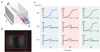
Figure S1: Modeling an imperfect beam displacer. a. Schematic of a beam displacer (BD). b. Interference pattern obtained from the output beams after projecting on circular polarization (and with a circularly polarized input beam). c. Geometrical phase curves for different values of the deviation angle $\beta$.

References

- Berry [1984] M. V. Berry, Quantal Phase Factors Accompanying Adiabatic Changes, Proceedings of the Royal Society A: Mathematical, Physical and Engineering Sciences 392, 45 (1984).
- Pancharatnam [1956] S. Pancharatnam, Generalized theory of interference, and its applications - part I, Proceedings of the Indian Academy of Sciences - Section A 44, 247 (1956).
- Berry and Klein [1996] M. V. Berry and S. Klein, Geometric phases from stacks of crystal plates, J.Mod.Opt 43, 165 (1996).
- Chruscinski and Jamiolkowski [2004] D. Chruscinski and A. Jamiolkowski, Geometric phases in classical and quantum mechanics (Birkhäuser Basel, 2004).
- Cohen et al. [2019] E. Cohen, H. Larocque, F. Bouchard, F. Nejadsattari, Y. Gefen, and E. Karimi, Geometric phase from Aharonov–Bohm to Pancharatnam–Berry and beyond, Nature Reviews Physics 1, 437 (2019).
- Bomzon et al. [2002] Z. Bomzon, G. Biener, V. Kleiner, and E. Hasman, Space-variant pancharatnam–berry phase optical elements with computer-generated subwavelength gratings, Optics letters 27, 1141 (2002).
- Bliokh et al. [2019] K. Y. Bliokh, M. A. Alonso, and M. R. Dennis, Geometric phases in 2d and 3d polarized fields: geometrical, dynamical, and topological aspects, Reports on Progress in Physics 82, 122401 (2019).
- Rubano et al. [2019] A. Rubano, F. Cardano, B. Piccirillo, and L. Marrucci, Q-plate technology: a progress review, JOSA B 36, D70 (2019).
- Jisha et al. [2021] C. P. Jisha, S. Nolte, and A. Alberucci, Geometric phase in optics: from wavefront manipulation to waveguiding, Laser & Photonics Reviews 15, 2100003 (2021).
- Longuet-Higgins et al. [1958] H. C. Longuet-Higgins, U. Öpik, M. H. L. Pryce, and R. A. Sack, Studies of the jahn-teller effect .ii. the dynamical problem, Proceedings of the Royal Society of London. Series A. Mathematical and Physical Sciences 244, 1 (1958).
- Zak [1989] J. Zak, Berry’s phase for energy bands in solids, Physical review letters 62, 2747 (1989).
- Resta [2000] R. Resta, Manifestations of berry’s phase in molecules and condensed matter, Journal of Physics: Condensed Matter 12, R107 (2000).
- Nayak et al. [2008] C. Nayak, S. H. Simon, A. Stern, M. Freedman, and S. D. Sarma, Non-abelian anyons and topological quantum computation, Reviews of Modern Physics 80, 1083 (2008).
- Fradkin [2013] E. Fradkin, Field theories of condensed matter physics (Cambridge University Press, 2013).
- Resta [1994] R. Resta, Macroscopic polarization in crystalline dielectrics: the geometric phase approach, Reviews of modern physics 66, 899 (1994).
- Asbóth et al. [2016] J. K. Asbóth, L. Oroszlány, and A. Pályi, A short course on topological insulators, Lecture notes in physics 919, 166 (2016).
- Hasan and Kane [2010] M. Z. Hasan and C. L. Kane, Colloquium: topological insulators, Reviews of modern physics 82, 3045 (2010).
- Garrison and Wright [1988] J. Garrison and E. Wright, Complex geometrical phases for dissipative systems, Physics Letters A 128, 177 (1988).
- Dattoli et al. [1990] G. Dattoli, R. Mignani, and A. Torre, Geometrical phase in the cyclic evolution of non-hermitian systems, Journal of Physics A: Mathematical and General 23, 5795 (1990).
- El-Ganainy et al. [2018] R. El-Ganainy, K. G. Makris, M. Khajavikhan, Z. H. Musslimani, S. Rotter, and D. N. Christodoulides, Non-hermitian physics and pt symmetry, Nature Physics 14, 11 (2018).
- Cho et al. [2019] Y.-W. Cho, Y. Kim, Y.-H. Choi, Y.-S. Kim, S.-W. Han, S.-Y. Lee, S. Moon, and Y.-H. Kim, Emergence of the geometric phase from quantum measurement back-action, Nature Physics , 1 (2019).
- Gebhart et al. [2020] V. Gebhart, K. Snizhko, T. Wellens, A. Buchleitner, A. Romito, and Y. Gefen, Topological transition in measurement-induced geometric phases, Proceedings of the National Academy of Sciences 117, 5706 (2020), 1905.01147 .
- Snizhko et al. [2021a] K. Snizhko, P. Kumar, N. Rao, and Y. Gefen, Weak-Measurement-Induced Asymmetric Dephasing: Manifestation of Intrinsic Measurement Chirality, Physical Review Letters 127, 170401 (2021a), 2006.13244 .
- Snizhko et al. [2021b] K. Snizhko, N. Rao, P. Kumar, and Y. Gefen, Weak-measurement-induced phases and dephasing: Broken symmetry of the geometric phase, Physical Review Research 3, 043045 (2021b), arXiv:2006.14641 .
- Wang et al. [2022] Y. Wang, K. Snizhko, A. Romito, Y. Gefen, and K. Murch, Observing a topological transition in weak-measurement-induced geometric phases, Physical Review Research 4, 023179 (2022), 2102.05660 .
- Bolduc et al. [2013] E. Bolduc, N. Bent, E. Santamato, E. Karimi, and R. W. Boyd, Exact solution to simultaneous intensity and phase encryption with a single phase-only hologram, Opt. Lett. 38, 3546 (2013).
- Jacobs [2014] K. Jacobs, Quantum Measurement Theory and its Applications (Cambridge University Press, Cambridge, 2014).
- Coley [1999] D. A. Coley, An introduction to genetic algorithms for scientists and engineers (World Scientific Publishing Company, 1999).