Black holes and nilmanifolds: quasinormal modes as the fingerprints of extra dimensions?

Abstract

We investigate whether quasinormal modes (QNMs) can be used in the search for signatures of extra dimensions. To address a gap in the Beyond the Standard Model (BSM) literature, we focus here on higher dimensions characterised by negative Ricci curvature. As a first step, we consider a product space comprised of a four-dimensional Schwarzschild black hole space-time and a three-dimensional nilmanifold (twisted torus); we model the black hole perturbations as a scalar test field. We suggest that the extra-dimensional geometry can be stylised in the QNM effective potential as a squared mass-like term representing the Kaluza-Klein (KK) spectrum. We then compute the corresponding QNM spectrum using three different numerical methods, and determine a possible “detectability bound” beyond which KK masses cannot be detected using QNMs.

1 Introduction

Quasinormal modes (QNMs), the damped and discrete oscillations in space-time that emanate from a perturbed body as it returns to an equilibrium state Vishveshwara1970 ; Press1971 , have served for several decades as a theoretical means of studying $d$-dimensional black hole space-times as well as a testing ground for the development of numerical simulations and techniques. Quantum gravity conjectures, modified theories of gravity, stability analyses of naked singularities and novel space-times, the development of numerical relativity simulations, and the explorations of the gauge-gravity duality are but a few of the avenues of research made accessible by black hole QNMs (see Refs. refNollert1999 ; refKokkotasRev ; refFerrari2008 ; refBertiCardoso ; refKonoplyaZhidenkoReview for reviews).

From the astrophysical perspective, quasinormal frequencies (QNFs) $\omega$ lead directly to insights about the nature of their black hole source. Specifically, the oscillation frequency $\mathbb{R}e\{\omega\}$ and damping $\tau=-1/\mathbb{I}m\{\omega\}$ of the QNFs are uniquely determined by the characteristic black hole properties of mass $M$, spin $a$, and charge $Q$ Echeverria1989_BHpropertiesestimate , in accordance with the no-hair conjecture applicable to final-state black holes Gravitation1973 . This has earned QNMs the epithet “black hole fingerprints” refKonoplyaZhidenkoReview . As such, furthering our understanding of black holes in turn allows us to explore gravity in the relatively untested strong regime, complementing extant results obtained from experiments in low-velocity linear regimes Stairs2003_GRpulsarTests ; Will2009_GRstellarTests ; refWillReview2014 ; Berti2015_TestingGRastro .

Mathematically, QNMs can be structured as an eigenvalue problem subjected to physically-motivated boundary conditions and dependent strictly on the features of the black hole space-time and the effective potential of the perturbing field. If we consider a static black hole (in an asymptotically-flat space-time) through the classical lens, radiation is purely in-going at the event horizon and purely out-going at spatial infinity; the black hole geometry is characterised solely by its mass NoHair_Schwarzschild while the effective potential depends on the spin of the oscillating field and the multipolar (angular momentum) number $\ell$. For each $\ell$ there are infinitely many overtones $n$ labelling the QNF in increasing multiples of $\mathbb{I}m\{\omega\},$ with the $n=0$ fundamental mode representing the least-damped and thus longest-lived QNM.

On the basis of spherical symmetry and time independence, the QNM behaviour in static black hole space-times can be shown to reduce to a simple radial wave equation, as first demonstrated in Refs. refRW ; refZerilli for the Schwarzschild case. A wide range of methods have been developed to determine QNM solutions from such wave equations, including methods that are “exact” (e.g. direct integration methods DavisPrice1971 ; Price1994 , the continued fraction method refLeaver1985 , pseudospectral methods Dias2009_Paraspectral1 ; Dias2009_Paraspectral2 , etc.) and numerical (e.g. the asymptotic iteration method refAIM_OG ; refAIM , the Horowitz-Hubeny approach HorowitzHubeny , etc.). Of these, we highlight (i) inverse-potential methods that approximate the effective potential with an inverse Pöschl-Teller potential PoschlTellerPotential for which bound-state solutions are known to determine the QNF spectrum PoschlTellerMethod ; (ii) WKB-based methods that adapt the semi-class- ical technique to the QNM problem to compute QNFs in the $\ell\geq n$ regime refBHWKB0 ; refBHWKB0.5 ; refBHWKB1 at sixth-order Konoplya2003 and beyond (see Ref. Konoplya2019 ); (iii) photon-orbit methods such as the inverse multipolar expansion method refDolanOttewill2009 that harnesses the known link between QNMs and unstable null geodesics refGoebel1972 to construct an iterative technique to solve the wave-like radial equation with increasing accuracy for large values of $\ell$ refOurLargeL . This is by no means an exhaustive list; for further insights, we refer the reader to Refs. refBertiCardoso ; refKonoplyaZhidenkoReview ; Grandclement2007_Spectral ; Dias2015_Num .

Today, we find ourselves in the unprecedented position wherein which we can observe this gravitational radiation. To date, the LIGO-Virgo-KAGRA (LVK) collaboration has confirmed 90 gravitational-wave (GW) events with a probability of astrophysical origin
$p_{astro}\leavevmode\nobreak\ >\leavevmode\nobreak\ 0.5$ refLIGO2018Run1 ; refLIGO2020Run2 ; refLIGO2021Run3a ; refLIGOrecentRun3b , providing us with the novel opportunity to scrutinise general relativity (GR) in the relativistic strong-field regime and placing us firmly in the era of GW astronomy. While this has immediate astrophysical Berti2015_TestingGRastro and cosmological LVK2021_Cosmic relevance, there is a significant interest in the theoretical implications of GWs Yunes2016_GW15implications and the fundamental physics insights they might provide Barack2018_GWfunphys .

This is in part due to their weakly-interacting nature: GWs propagate unimpeded through the universe, piercing both the cosmic microwave and cosmic neutrino backgrounds, possibly providing unique insights into the inflationary epoch and beyond Weir2017_GWsFOPTreview ; Cai2017_GWphysics ; Nature_GWreview . These high and ultra high frequency stochastic GWs correspond to energies of the TeV range and higher, towards the Planck scale; in this way, GWs serve as a complementary laboratory to collider physics experiments Aggarwal2020_HighFGWs ; Alves_GWLHCComplement ; Caldwell2022_GWLHCSnowMass . Searches for new physics focused on early-universe dynamics are well-underway, with examples such as Ref. Huang2020_PatiSalamDynamics demonstrating that models based at scales of Grand Unified Theories can be good candidates for detection via next-generation GW detectors refGWsensitivity . This has encouraged new lines of inquiry into cosmic strings Chigusa2020_GWGUT ; King2021_GWGUT , leptogenesis White2019_GWGUT , dark matter Buchmuller2019_GWGUT , and other beyond the Standard Model (BSM) challenges.

GWs are also being applied to searches for extra dimensions (see Refs. Yu2019 ; Cardoso2019_GWsEDsKK ; Kwon2019_GWsCompactifiedEDs ). Compact extra dimensions feature a variety of different geometries (Ricci-flat AndriotGomez2017_EDsignGWs ; Du2021_GWsCompactifiedEDs ; Ferko2022_GWsCompactifiedEDs , toroidal AndriotTsimpis2019_WarpGWs , warped toroidal AndriotTsimpisMarconnet2021_WarpGWs extra dimensions, etc.). These, on the other hand, have so far predicted GWs whose frequencies are of the order of $10^{12}-10^{14}$ Hz, far exceeding the $10^{3}-10^{4}$ Hz upper limit of present and planned detectors Nature_GWreview ; Aggarwal2020_HighFGWs .

Here, however, we are guided by the capabilities of modern detectors, and investigate whether we can exploit present-day GW observations to infer constraints on new physics. In particular, we shall focus on binary black hole collisions, where the post-merger ringdown phase is dominated by quasinormal ringing Berti2007 . For this reason, we can apply known theoretical and numerical QNM techniques to experimental observations. Logistically, we concentrate on black holes because the dynamics of binary black hole collisions have been studied extensively Berti2007 ; refFerrari2008 ; refBroeck2013 ; the success of the LVK collaboration is a testament to the gravitational waveform modelling expertise, Bayesian statistical analysis techniques, and experimental prowess carefully honed over several decades (see Ref. refLIGOguide for the LVK collaboration’s guide on data acquisition and processing).

Furthermore, since the signal-to-noise ratio of the post-merger signal is usually fairly low and therefore not always characterisable LIGO2019_GWTC1-GRtest ; LIGO2020_GWTC2-GRtest_pyRing3 ; LIGO2021_GWTC3-GRtest , the higher-mass and louder black hole merger events are more likely to produce good candidates for ringdown analyses. The first detected GW event GW150914 refLIGO ; GW150914properties was sufficiently loud to accommodate a QNM study, so we shall restrict our discussion to this event within this work, unless otherwise stated.

Current searches for evidence of new physics from available GW observations are dominated by model-agnostic null tests for deviations from GR predictions. These include: consistency checks between data and GR-based models for the evolution of a merger event; tests of the generation and propagation of GWs, where the latter involves searching for modifications to the dispersion relation and in turn constraining the Compton wavelength associated with the graviton mass; tests for additional polarisation modes beyond the tensor plus and cross modes predicted by GR; analyses of the post-merger properties for parametric deviations from GR LIGO2016_TestingGRGW150914 ; LIGO2019_GWTC1-GRtest ; LIGO2020_GWTC2-GRtest_pyRing3 ; LIGO2021_GWTC3-GRtest , etc. At present, there have been no statistically significant deviation from GR reported.

However, this latter category of testing has been a subject of growing fascination, and motivates investment in more precise measurements of QNFs Berti2020_LISAringdownMultipolar ; OtaChirenti2021_BHspectroscopyPresentFuture ; Bhagwat2021_BHspectroscopyPresentFuture . Furthermore, hopes for the establishment of black hole spectroscopy Berti2005_BHspectroscopy are beginning to be realised: although the $n=0$, $\ell=2$ mode is known to dominate the QNM spectrum, higher harmonics Carullo2019_pyRing1 ; Capano2021_MultipolarQNMsObserved and overtones Cotesta2022_OvertonesRingdown are being investigated. Tests of the no-hair conjecture are of particular interest Carullo2018_NoHairTests ; refNoHair_pyRing ; refNoHair_pyRing2 ; Isi2022_GW150914again ; Ghosh:2021_QNMconstraints , as a violation thereof may be evidence of an exotic object or new physics.

As such, we shall focus here on this use of parametric deviations from GR in the QNF spectrum in an attempt to outline a search for extra dimensions. In fact, there have already been considerations for extra dimensions using black hole QNMs, concentrated for example on the five-dimensional (5D) Randall-Sundrum II RSmodel2 model: through the formalism of Shiromizu et al. Shiromizu1999_Einstein3Brane and Dadhich et al., a 4D effective framework can be established from a 5D general relativity construction, leading to a (neutral) black hole solution that resembles the (charged) Reissner-Nordström metric. The so-called tidal charge $\beta=Q^{2}/(4M^{2})$ is a manifestation of the influence of the extra dimension. In Ref. Mishra2021_QNMsEDs , this is the observable utilised to constrain extra dimensions, but is found to disfavour extra dimensions.

It is not clear how to extend the Shiromizu et al. formalism to a broader category of extra-dimensional models with $d>5$, nor is it obvious whether this tidal charge observable can be probed for general cases. Moreover, it may be that alternate geometries could lead to successful GW detection. Bearing these points in mind, we shall consider as an example a particularly simple partially-compactified setup: a direct product space featuring a four-dimensional Minkowski space-time and a three-dimensional negative compact space $\mathcal{M}_{4}\times\mathcal{N}_{3}$. Within this space-time, we shall embed a four-dimensional Schwarzschild black hole. The higher-dimensional component will then be comprised of a twisted torus $-$ known as a nilmanifold $-$ constructed from the non-trivial fibrations of layered tori. The nilmanifold is one of the few geometries that allows for analytic calculations of mass spectra and Kaluza-Klein (KK) reductions Andriot2016_TowardsKK , and boasts a number of phenomen- ologically-interesting properties that we shall discuss in section 2.1.

While the higher-dimensional manifold is highly specific, we shall show that the variable-separable nature of our extra-dimensional space-time in the absence of coupling between components of $\mathcal{M}_{4}$ and $\mathcal{N}_{3}$ and the QNM problem we consider, allows for a KK reduction that expresses the extra-dimensional behaviour as a mass-like term that can be incorporated into the QNM effective potential. We shall demonstrate how this enables the application of QNM literature on massive oscillating fields, as well as studies on parametric deviations from GR employed by the LVK collaboration. In so doing, we lay the groundwork for an additional avenue through which we may probe GW observations for model-agnostic extra-dimensional signatures.

The structure of this paper is as follows. In section 2, we define the “Schwarzschild-nilmanifold” setup we investigate: we outline the interesting features and the construction of the nilmanifold, as well as the construction of the partially-compactified seven-dimensional (7D) metric and the scalar field we use to explore it. There, we shall derive a 4D effective potential in which the higher-dimensional character is encoded in an effective mass term. In so doing, we recreate the problem of massive scalar QNMs: a scenario that has been used as a case study for numerical development in the QNM literature.

In section 3, we compute the QNF spectrum using the three numerical methods highlighted, viz. the inverse Pöschl-Teller potential method, the WKB method, and the inverse-$\ell$ method. We include also a discussion on how the QNF spectrum is affected by the mass-like term. In this way, we shall determine an upper bound under which detectable black hole QNMs may serve as an appropriate probe for extra dimensions in this construction. To constrain this mass-like parameter further, we introduce bounds from studies on the parametric deviation of GW data from GR predictions, using the most stringent results published by the LVK collaboration LIGO2021_GWTC3-GRtest . This step shall be carried out in section 4. By comparing the magnitude of the deviation from GR in the ringdown phase with the deviations in a the QNF spectrum caused by our introduction of the effective mass term, we are able to place naïve constraints on detectable QNFs harbouring extra-dimensional signatures. In other words, we demonstrate a plausible detectability bound on the observation of KK masses using QNFs. While our interest lies specifically in the case of negative extra-dimensional components, this result is agnostic to the extra-dimensional scalar curvature and therefore applies to a wide variety of extra-dimensional setups featuring compact spaces. We note, however, that our objective here is not to supply a definitive constraint on extra dimensions. Rather, we suggest a pragmatic method by which QNFs can be repurposed for BSM searches through combining known techniques and available GW data.

2 A Schwarzschild-nilmanifold extra-dimensional setup

Compact negative-curvature spaces (i.e. spaces with negative Ricci scalar curvature) have been interrogated extensively within the mathematical literature Needham2012_VisualCA ; Berger2013_PanoramicRiemannian . Among members of the string theory community, a burgeoning interest in such spaces is developing in the wake of a recent observation that negatively-curved manifolds are a requirement for classical de Sitter solutions with orientifold planes Haque2008_NegCurve1 ; Andriot2016_NegCurve2 ; AndriotMarconnet2022_10dAdS . In the context of particle physics, extra-dimensional models characterised by partial or total negative scalar curvature remain comparatively under-explored.

Phenomenologically, studies on compact hyperbolic spaces are promising for their capacity to include cosmological observations such as homogeneity and flatness Starkman2001_CosmoED ; Chen2003_CosmoHypED ; Neupane2003_CosmoExpPot . Moreover, these models could be used to address the hierarchy problem between the Planck and the electroweak scale by virtue of their geometrical properties. Compact negative-curvature spaces possess two characteristic length scales: $\ell_{\rm c}$, associated with local properties like the curvature and fixed by the equations of motion, and $\ell_{\rm G}$, associated with global properties like the volume and independent of the equations of motion. Their volume grows exponentially with $\ell_{\rm c}/\ell_{\rm G}$, leading to an exponential reduction of the Planck length, which in turn yields a natural explanation for the perceived discrepancy in energy scales OrlandoPark2010_HyperbolicEDatLHC . Furthermore, the KK mass spectra associated with such spaces are usually similar to those of Randall-Sundrum models RSmodel1 in that they accommodate the electroweak-Planck scale hierarchy without introducing light KK modes OrlandoPark2010_HyperbolicEDatLHC .

Motivated by these implications, a series of investigations Andriot2016_TowardsKK ; AndriotTsimpis2018_Laplacian ; IP2I2020_Nilmanifolds ; Deandrea2022_GHnilmanifolds ; Deandrea2022_Diracnilmanifolds have focused model-building efforts on a compact, negatively-curved manifold whose tangent vectors form a Lie algebra that is nilpotent viz. a nilmanifold $\mathcal{N}_{3}$ (see Refs. Andriot2015_Solvmanifolds ; Bock2009_Solvmanifolds ). In the sections that follow, we shall outline how the nilmanifold is constructed from the Heisenberg algebra and demonstrate the KK expansion of a scalar field in this context, as established in Ref. Andriot2016_TowardsKK . With these elements in place, we may proceed to the construction of our Schwarzschild-nilmanifold setup, and the KK reduction that allows us to treat the oscillations travelling through the 7D product space-time as a massive 4D scalar field.

2.1 Algebra, geometry, and a 3D scalar field

Any Lie group of dimension $d$ can be understood as a $d$-dimensional differentiable manifold. Under certain conditions (see Ref. Grana2006_TwistedToriReview for a review), a solvable Lie group $G$ can be divided by a lattice $\Gamma$, a discrete subgroup of $G$, to construct a compact solvmanifold (i.e. a twisted torus) by means of discrete identifications Andriot2010_Thesis . Nilpotent groups are a special subclass of solvable groups. For them, the compactness criterion requires the structure constants to be rational in some basis Malcev1951 . We refer to their corresponding compact manifolds as nilmanifolds.

Consider the $d$-dimensional Lie algebra $\mathfrak{g}$ generated by the vectors $\{Z_{a},a=1,...,d\}$ satisfying

$$[Z_{b},Z_{c}]=f\indices{{}^{a}_{bc}}Z_{a}\;.$$ (2.1)

Here, the structure constants satisfy $f\indices{{}^{a}_{bc}}=-f\indices{{}^{a}_{cb}}$. The corresponding $d$-dimensional manifold admits a globally-defined orthonormal frame $\{e^{a},a=1,...,d\}$ (where this basis defines the dual space of one-forms $\mathfrak{g}^{\star}$). This frame obeys the Maurer-Cartan equation

$$\text{d}e^{a}=-\frac{1}{2}f\indices{{}^{a}_{bc}}e^{b}\wedge e^{c}=-\sum_{b<c}f\indices{{}^{a}_{bc}}e^{b}\wedge e^{c}\;,$$ (2.2)

with the exterior derivative d. Since the dual space $\mathfrak{g}^{\star}\approx T_{e}G^{\star}$, $\{e^{a},a=1,...,d\}$ provides $-$ by left invariance $-$ a basis for the cotangent space $T_{x}G^{\star}$ at every point $x\in G$, the one-forms are globally defined on the manifold. These one-forms will have their non-trivial identification through the “lattice action” when $G$ is divided by $\Gamma$. Note that $f\indices{{}^{a}_{bc}}$ is related to the spin connection.

In flat indices and for a unimodular Lie algebra, the Ricci tensor is given by

$$\mathcal{R}_{cd} = \frac{1}{2}\Big{(}-f\indices{{}^{b}_{ac}}f\indices{{}^{a}_{bd}}-\delta^{bg}\delta_{ah}f\indices{{}^{h}_{gc}}f\indices{{}^{a}_{bd}}$$ (2.3)

$$+\frac{1}{2}\delta^{ah}\delta^{bj}\delta_{ci}\delta_{dg}f\indices{{}^{i}_{aj}}f\indices{{}^{g}_{hb}}\Big{)}\;,$$

with $\delta_{ab}$ serving as a Euclidean metric. For the nilpotent algebra, and thus for the nilmanifold case, the first term vanishes. The Ricci tensor is thus nowhere-vanishing and the corresponding Ricci scalar emerges as

$$\mathcal{R}=-\frac{1}{4}\delta_{ad}\delta^{be}\delta^{cg}f\indices{{}^{a}_{bc}}f\indices{{}^{d}_{eg}}\;.$$ (2.4)

The Ricci scalar is strictly negative.

From Eq. (2.2), we can see that $d=3$ is the lowest dimensionality for which this expression is non-trivially satisfied. For $d=3$, there is the trivial Abelian algebra that leads to a three-torus, as well as three different solvable algebras. Of these, one is nilpotent: the Heisenberg algebra

$$[Z_{1},Z_{2}]=-\mathtt{f}Z_{3}\;,\hskip 8.5359pt[Z_{1},Z_{3}]=[Z_{2},Z_{3}]=0\;,$$ (2.5)

with $\mathtt{f}=-f^{3}_{12}\neq 0$ such that the Maurer-Cartan equation becomes

$$\text{d}e^{3}=\mathtt{f}e^{1}\wedge e^{2}\;,\hskip 8.5359pt\text{d}e^{1}=0\;,\hskip 8.5359pt\text{d}e^{2}=0\;.$$ (2.6)

The only nonzero structure constant $\mathtt{f}=-f^{3}_{\;\;\;12}\in\mathbb{R}$ is the geometric flux serving as the nilmanifold’s twist parameter. The corresponding geometric properties of the nilmanifold can be relayed through the Maurer-Cartan equation Eq. (2.6), from which we define

$$e^{1}=r^{1}\mathrm{d}y^{1}\;,\;\;e^{2}=r^{2}\mathrm{d}y^{2}\;,\;\;e^{3}=r^{3}(\mathrm{d}y^{3}+Ny^{1}\mathrm{d}y^{2})$$ (2.7)

for the constant radii $r^{1,2,3}>0$, angular coordinates $y^{m}\in[0,1]$, and the integer $N=r^{1}r^{2}\mathtt{f}/r^{3}$ Andriot2016_TowardsKK .

The discrete identifications that make the compactification possible are

$$y^{1}\sim y^{1}+n^{1}\;,\;\;y^{2}\sim y^{2}+n^{2}\;,\;\;y^{3}\sim y^{3}+n^{3}-n^{1}Ny^{2}\;,$$ (2.8)

for $n^{m=1,2,3}\in[0,1].$ In other words, these identifications correspond to the lattice action responsible for establishing $\mathcal{N}_{3}$ as a nilmanifold. Eq. (2.8) leaves Eq. (2.7) invariant.

In this way, the compact manifold is fully characterised as a twisted $S^{1}$ fibration over layered tori $T^{2}$. The twist is along the fibre coordinate $y^{3}$, while the base is parameterised by the coordinates $(y^{1},y^{2})$. Physically, $y^{m=1,2,3}$ are angles defined on $[0,1]$. The constant radii $r^{m}$ have units of length, the coordinates $y^{m}$ are dimensionless, and $\mathtt{f}$ has units of inverse length (i.e. energy).

The most general left-invariant metric for the nilmanifold is given by

$$\text{d}s^{2}=\delta_{ab}E^{a}E^{b}\;,\;\;\;E^{a}=\left(L^{-1}\right)\indices{{}^{a}_{b}}e^{b},$$ (2.9)

where we use $E^{a}$ to denote the one-forms related to the orthonormal basis $e^{a}$ through the constant $GL(3,\mathbb{R})$ transformation $L$.

To demonstrate the construction of the scalar mass spectrum, we shall consider the simplified special case in which $r^{m}=1$ and $\mathtt{f}=1$. The nilmanifold metric then becomes

$$\mathrm{d}s^{2}_{\rm nil}=\delta_{ab}e^{a}e^{b}=(\mathrm{d}y^{1})^{2}+(\mathrm{d}y^{2})^{2}+(\mathrm{d}y^{3}+y^{1}\mathrm{d}y^{2})^{2}\;.$$ (2.10)

To understand the behaviour of a scalar field on this space, we consider the massive Klein-Gordon equation. Let us begin with the Laplacian

$$\nabla^{2}\Phi=\frac{1}{\sqrt{g}}\delta_{m}\left(\sqrt{g}g^{mn}\delta_{n}\Phi\right)\;,$$ (2.11)

where the determinant $\sqrt{g}=r^{1}r^{2}r^{2}$ reduces to 1 in our simplified metric. We may write

$$\nabla^{2}u=\left(\partial_{1}^{2}+\left(\partial_{2}-y^{1}\partial_{3}\right)^{2}+\partial_{3}^{2}\right)u\;,$$ (2.12)

as we shall consider the expansion of $u$ on the space of functions invariant under Eq. (2.8), beginning with the functions depending only on the base coordinates $(y^{1},y^{2})$. In this case, the Laplacian is easily diagonalised:

$$\left(\nabla^{2}+\upmu^{2}_{\beta,\gamma}\right){\tilde{v}}_{\beta,\gamma}=0\;,$$ (2.13)

where we define

$$\tilde{v}_{\beta,\gamma}(y^{1},y^{2})=e^{2\pi i\beta y^{1}}e^{2\pi i\gamma y^{2}}\;,$$ (2.14)

for $\beta,\gamma\in\mathbb{Z}$, as invariant under Eq. (2.8), and the Klein-Gordon masses as

$$\upmu^{2}_{\beta,\gamma}=4\pi^{2}\left(\beta^{2}+\gamma^{2}\right)\;.$$ (2.15)

We can present a more generalised expression using the Weil-Brezin-Zak transforms Thangavelu_HA for a basis of invariant functions $u_{\kappa,\lambda}$,

$$u_{\kappa,\lambda}(y^{1},y^{2},y^{3}) = e^{2\pi\kappa i(y^{3}+y^{1}y^{2})}e^{2\pi\lambda iy^{1}}$$

$$\times\sum_{\sigma}e^{2\pi\kappa\sigma iy^{1}}f(y^{2}+\sigma)\;,$$

for $\kappa,\lambda,\sigma\in\mathbb{Z}$. Since $u_{\kappa,\lambda}$ is invariant under Eq. (2.8) for all values of $f(x)$, the functions remain well-defined across our nilmanifold $\mathcal{N}_{3}$. Upon substituting Eq. (2.1) into Eq. (2.12), we obtain

$$\nabla^{2}u_{\kappa,\lambda} = e^{2\pi\kappa i(y^{3}+y^{1}y^{2})}e^{2\pi\lambda iy^{1}}\sum_{\sigma}e^{2\pi\kappa\sigma iy^{1}}$$

$$\times \left[\partial_{2}^{2}-4\pi^{2}\left(\kappa^{2}+(\kappa(y^{2}+\sigma)+\lambda)^{2}\right)\right]f(y^{2}+\sigma)\;,$$

where we require that $\kappa\neq 0$ to retain the $y^{3}$-dependent terms.

If we introduce $z_{\sigma}=y^{2}+\sigma+\lambda/\kappa$ and $g(z_{\sigma})=f(y^{2}+\sigma)$, we can rewrite the above Laplacian as

$$\nabla^{2}u_{\kappa,\lambda} = e^{2\pi\kappa i(y^{3}+y^{1}y^{2})}e^{2\pi\lambda iy^{1}}\sum_{\sigma}e^{2\pi\kappa\sigma iy^{1}}$$

$$\times \left[\partial_{z_{\sigma}}^{2}-(2\pi\kappa)^{2}\left(z_{\sigma}^{2}+1)\right]g(z_{\sigma})\right]\;.$$

From the normalised Hermite functions

$$X_{\nu}(z)=e^{-z^{2}/2}H_{\nu}(z)\;,\;\;\nu\in\mathbb{N}\;,$$ (2.19)

where $H_{\nu}$ represents the Hermite polynomials, we may define

$$X_{\nu}^{\rho}(z)=|\rho|^{1/4}X_{\nu}(|\rho|^{1/2}z)$$ (2.20)

for $\rho\in\mathbb{R}^{*}$ Thangavelu_HA . By the properties of Hermite polynomials, Eq. (2.20) satisfies the differential equation

$$(\partial^{2}_{z}-\rho^{2}z^{2})X^{\rho}_{\nu}(z)=-(2\nu+1)|\rho|X^{\rho}_{\nu}(z)\;.$$ (2.21)

With the insertion of $g(z_{\sigma})=X^{2\pi\kappa}_{\nu}(z_{\sigma})$ into Eq. (2.1), we obtain the 3D Klein-Gordon equation

$$\left(\nabla^{2}+M^{2}_{\kappa,\lambda,\nu}\right)\tilde{u}_{\kappa,\lambda,\nu}=0\;,$$ (2.22)

where the masses and wavefunctions are, respectively,

$$M^{2}_{\kappa,\lambda,\nu}=(2\pi\kappa)^{2}\left(1+\frac{2\nu+1}{2\pi|\kappa|}\right)\;,$$ (2.23)

$$\tilde{u}_{\kappa,\lambda,\nu}(y^{1},y^{2},y^{3}) = e^{2\pi\kappa i(y^{3}+y^{1}y^{2})}e^{2\pi\lambda iy^{1}}\sum_{\sigma}e^{2\pi\kappa\sigma iy^{1}}$$ (2.24)

$$\times X^{2\pi\kappa}_{\nu}\left(y^{2}+\sigma+\frac{\lambda}{\kappa}\right)$$

for $\sigma\in\mathbb{Z}$, $\nu\in\mathbb{N}$, $\kappa\in\mathbb{Z}^{*}$, and $\lambda=0,...,|\kappa|-1$. The range of $\lambda$ is derived from the fact that $\lambda$ itself is defined modulo $\kappa$, which in turn is a consequence of the identity

$$\tilde{u}_{\kappa,\lambda+\kappa\tau,\nu}(y^{1},y^{2},y^{3})=\tilde{u}_{\kappa,\lambda,\nu}(y^{1},y^{2},y^{3})\;\;\forall\;\tau\in\mathbb{Z}\;.$$ (2.25)

By virtue of Eq. (2.23)’s independence of $\lambda$, there exists a mass degeneracy. The wavefunctions are parameterised by a finite number of inequivalent values of $\lambda$ such that the level of the degeneracy is $|\kappa|.$ Note that only one zero-mode (i.e. with vanishing mass) exists for this Klein-Gordon equation, $\tilde{v}_{0,0}$, corresponding to the modes of the torus base.

We conclude this discussion on the nilmanifold space with the physical spectrum associated with a scalar field propagating on $\mathcal{N}_{3}$. This is achieved by reintroducing dimensional parameters $r^{m}$ and $\mathtt{f}$ Andriot2016_TowardsKK . We may distinguish between torus modes,

$$v_{\beta,\gamma}(y^{1},y^{2}) = \frac{1}{\sqrt{V}}e^{2\pi i\beta y^{1}}e^{2\pi i\gamma y^{2}}\;,$$ (2.26)

$$\upmu^{2}_{\beta,\gamma} = \beta^{2}\left(\frac{2\pi}{r^{1}}\right)^{2}+\gamma^{2}\left(\frac{2\pi}{r^{2}}\right)\;,$$ (2.27)

and fibre modes,

$$u_{\kappa,\lambda,\nu}(y^{1},y^{2},y^{3}) = \sqrt{\frac{r^{2}}{|N|V}}\frac{1}{\sqrt{2^{\nu}\nu!\sqrt{\pi}}}e^{2\pi\kappa i(y^{3}+Ny^{1}y^{2})}$$ (2.28)

$$\times e^{2\pi\lambda iy^{1}}\sum_{\sigma}e^{2\pi\kappa\sigma iy^{1}}X^{\rho}_{\nu}(w_{\sigma})\;,$$

$$M^{2}_{\kappa,\lambda,\nu} = \kappa^{2}\left(\frac{2\pi}{r^{3}}\right)^{2}+(2\nu+1)|\kappa|\frac{2\pi\mathtt{f}}{r^{3}}\;,$$ (2.29)

for which we define

$$\rho=\frac{2\pi\mathtt{f}}{r^{3}}\kappa\;,\hskip 8.5359ptw_{\sigma}=r^{2}\left(y^{2}+\frac{\sigma}{N}+\frac{\lambda}{N\kappa}\right)\;,$$

and the volume

$$V=\int d^{3}y\,\sqrt{g}=r^{1}r^{2}r^{3}\;.$$ (2.30)

The scalar spectrum on the nilmanifold contains a complete tower of modes on the torus that is independent of the fibre coordinate and radius. The fibre modes, whose mass spectrum is a function of the radial components and the curvature-related energy scale $\mathtt{f}$, have been shown to be tunable in Ref. Andriot2016_TowardsKK by varying parameters in the generalised case; the fibre modes can be made lighter than their toroidal counterparts and the energy gaps in the spectrum may be enhanced. From the structure of Eq. (2.29) itself, we understand that the fibre modes present with a unique mass spectrum: added to the typical $1/R$ Kaluza-Klein term is the novel $\mathtt{f}$-dependent term that enforces more finely-spaced modes, which follow a linear Regge trajectory. From the characteristic fibre-mode spectrum, we would expect a unique experimental signature.

To see clearly the distinctive spectrum of the nilmanifold, let us compare the fibre-mode masses of Eq. (2.29) to the KK masses of a standard compactification $M_{st;\kappa,\lambda,\nu}$ on a three-dimensional torus $\mathbb{T}^{3}$,

$$M^{2}_{st;\kappa,\lambda,\nu}=\kappa^{2}\left(\frac{2\pi}{r^{1}}\right)^{2}+\lambda^{2}\left(\frac{2\pi}{r^{2}}\right)^{2}+\nu^{2}\left(\frac{2\pi}{r^{3}}\right)^{2}\leavevmode\nobreak\ ,$$ (2.31)

where $\kappa$, $\lambda$, $\nu\in\mathbb{Z}$. For simplicity we shall take all internal radii to be equal, $r^{1}=r^{2}=r^{3}$. Moreover we shall consider a nilmanifold $\mathcal{N}_{3}$ with minimal twist, $N=1$. The ratio $R$ of excited KK masses to the lowest-lying one is then independent of the size of the radii of the internal manifold. For $\mathcal{N}_{3}$, $R^{2}_{nil}$ is given by

$$R^{2}_{nil}=\frac{M^{2}_{\kappa,\lambda,\nu}}{M^{2}_{1,0,0}}=\frac{2\pi\kappa^{2}+(2\nu+1)|\kappa|}{1+2\pi}\leavevmode\nobreak\ .$$ (2.32)

In contrast, for the standard $\mathbb{T}^{3}$, $R^{2}_{st}$ is given by

$$R^{2}_{st}=\frac{M^{2}_{st;\kappa,\lambda,\nu}}{M^{2}_{st;1,0,0}}=\kappa^{2}+\lambda^{2}+\nu^{2}\leavevmode\nobreak\ .$$ (2.33)

Table 1: The first few mass ratios $R_{nil}$ for the 3D nilmanifold $\mathcal{N}^{3}$, corresponding to Eq. (2.32) for $\kappa=1$.

$\nu$	$0$	$1$	$2$	$3$	$4$	$5$	$6$	$7$	$8$	$9$	$10$
$R^{2}_{nil}$	$1.0$	$1.3$	$1.6$	$1.8$	$2.1$	$2.4$	$2.6$	$2.9$	$3.2$	$3.5$	$3.7$

Table 2: The first few mass ratios $R^{2}_{nil}$ for the 3D nilmanifold $\mathcal{N}^{3}$, corresponding to Eq. (2.32) for $\kappa=2$.

$\nu$	$0$	$1$	$2$	$3$	$4$	$5$	$6$	$7$	$8$	$9$	$10$
$R^{2}_{nil}$	$3.7$	$4.3$	$4.8$	$5.4$	$5.9$	$6.5$	$7.0$	$7.6$	$8.1$	$8.7$	$9.2$

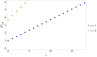
Figure 1: Plot of the mass ratios $R^{2}_{nil}\leq 6$ corresponding to Eq. (2.32) for $\mathcal{N}_{3}$ for $\kappa=1$ (blue) and $\kappa=2$ (orange).

Table 3: The first few mass ratios $R^{2}_{st}$ for the standard 3D torus $\mathbb{T}^{3}$, corresponding to Eq. (2.33).

$(\kappa\lambda\nu)$	$(100)$	$(110)$	$(111)$	$(200)$	$(210)$	$(211)$
$R^{2}_{st}$	$1$	$2$	$3$	$4$	$5$	$6$

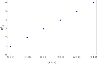
Figure 2: Plot of the ratios $R^{2}_{st}\leq 6$ corresponding to Eq. (2.33) and Table 3 for $\mathbb{T}^{3}$.

Since nilmanifolds allow for the possibility of analytically calculating the spectrum of propagating fields, they can be promising tools in the construction of effective BSM frameworks. Such models may be embeddable in string theory compactifications Andriot2016_TowardsKK . As mentioned in the introduction, recent investigations into GW signatures of compact extra dimensions predict observables at frequencies of the order of $10^{12}-10^{14}$ Hz and higher AndriotGomez2017_EDsignGWs ; AndriotTsimpis2019_WarpGWs ; AndriotTsimpisMarconnet2021_WarpGWs ; Yu2019 ; Cardoso2019_GWsEDsKK ; Kwon2019_GWsCompactifiedEDs $-$ several orders of magnitude beyond the $10^{4}$ Hz upper bound on modern detectors. However, these investigations suggest also that the KK GW spectrum is sensitive to changes in geometry. For example, introducing a non-trivial warp factor, as shown in Ref. AndriotTsimpisMarconnet2021_WarpGWs , can lower the first KK mass by at least 69% as compared against the standard KK spectrum on a torus $\mathbb{T}^{d}$. This is promising for the high-frequency GWs in extra-dimensional frameworks, as the relationship between frequency and KK mass implies that lower KK mass corresponds to GW frequencies closer to the sensitivity of modern instruments.

In Figs. 1 and 2, we see a similarly encouraging behaviour when we compare the fibre-mode spectrum with that of the standard torus modes. While we centre this work on the feasibility of detection with present-day data from the LVK collaboration, this effect motivates further investigation into the GWs propagating in nilmanifold spaces.

2.2 A Schwarzschild black hole and its scalar QNM

GR remains our most complete theory of gravity to date. Its underlying principle is the relationship it defines between the geometry and matter content of a space-time, expressed concisely through the Einstein field equations,

$$G_{MN}+\Lambda g_{MN}=\kappa_{D}\,T_{MN}\;.$$ (2.34)

Here, the Einstein tensor $G_{MN}$ expresses the local space-time curvature, $\kappa_{D}$ is the Einstein gravitational constant in $D$ dimensions, and $T_{MN}$ is the stress-energy tensor that defines the energy, momentum, and stress for the matter and field content within the local space-time Gravitation1973 . We set $G=c=1$, unless otherwise stated. In asymptotically-flat space-times, the cosmological constant $\Lambda$ vanishes. To describe the evolution of the metric and the fields, we utilise the $D$-dimensional Einstein-Hilbert gravitational action

$$\mathcal{S}=\frac{1}{2\kappa_{D}}\int\mathrm{d}^{D}x\,\sqrt{-g}\,\left(R+\mathcal{L}_{m}\right)\;,$$ (2.35)

where we use $\mathcal{L}_{m}$ to refer to all matter fields $\Psi$ within the space-time, and whose stress, energy, and momentum are encompassed by $T_{{MN}}$.

Within the context of GR, Birkhoff’s theorem stipulates that the most general spherically-symmetric vacuum solution of Eq. (2.34) is the Schwarzschild metric

$$\mathrm{d}s^{2}_{\rm BH} = g_{\mu\nu}^{\rm BH}\mathrm{d}x^{\mu}\mathrm{d}x^{\nu}=-f(r)\,dt^{2}+f(r)^{-1}\,dr^{2}$$ (2.36)

$$+r^{2}(d\theta^{2}+\sin^{2}d\phi^{2})\;,$$

where $f(r)=1-r_{H}/r$ and $r_{H}=2M$ is the Schwarzschild event horizon. For such a black hole, the length scale is defined by $M=mGc^{-2}$ for black hole mass $m^{\rm BH}$ Bekenstein2003_BHinfo , and is set to unity. The Schwarzschild coordinates $(t,r,\theta,\phi)$ are defined on the regions $t\in(-\infty,+\infty)$, $r\in(r_{H},+\infty)$, $\theta\in(0,\pi),$ and $\phi\in(0,2\pi)$; the tortoise coordinate $dr_{*}=dr/f(r)$ can be introduced to map the semi-infinite region of $(r_{H},+\infty)$ to $(-\infty,+\infty)$.

Eq. (2.36) describes an isolated, static, and neutral 4D black hole Gravitation1973 ; Chandrasekhar1983 that is fully characterised by its mass $M$ NoHair_Schwarzschild . Mathematically, black holes are therefore simple objects: they are pure geometry and do not require an equation of state to describe their evolution. Astrophysical black holes, however, are perpetually in a perturbed state: even if somehow isolated from the fields and matter in their immediate vicinity, they interact with the surrounding vacuum through Hawking radiation Hawking1975_HawkRad .

Black hole perturbation theory therefore considers a linearised approximation in which the black hole is described using

$$g^{\prime}_{\mu\nu}=g^{\rm BH}_{\mu\nu}+\delta_{\mu\nu}\;,$$ (2.37)

where the unperturbed black hole metric $g^{\rm BH}_{\mu\nu}$ is referred to as the “background” and the “perturbations” $\delta_{\mu\nu}$ are considered to be very small ($\delta_{\mu\nu}\ll g^{\rm BH}_{\mu\nu}$). Similarly, we may consider a perturbed background field $\Psi^{\prime}\leavevmode\nobreak\ =\leavevmode\nobreak\ \Psi^{\rm BG}+\psi$. We may then substitute $g^{\prime}_{\mu\nu}$ and $\Psi^{\prime}$ into Eq. (2.34), linearise the system of equations with respect to $\delta_{\mu\nu}$ and $\psi$, and thereby deduce the lineaised set of differential equations satisfied by the perturbations.

As detailed in Chandrasekhar’s book Chandrasekhar1983 , black hole QNM behaviour within a classical GR context can be inferred by substituting the perturbed metric, Eq. (2.37) and an ansatz into the Einstein field equations, and then solving for the vacuum solution under the physically-motivated QNM boundary conditions. The QNM ansatz and the number of ordinary differential equations required to describe the QNM propagation are derived from the symmetries of the background space-time: in the Schwarzschild case (static, non-rotating, and spherically-symmetric), the wave-function is written in variable-separable form,

$$\Phi^{s}_{n\ell m}(\mathbf{x})=\sum_{n}^{\infty}\sum_{\ell,m}^{\infty}\;\frac{\psi_{sn\ell}(r)}{r}\;Y^{s}_{m\ell}(\theta,\phi)\;,$$ (2.38)

and the angular behaviour is relayed through spherical harmonics

$$\nabla^{2}Y^{s}_{m\ell}(\theta,\phi)=-\frac{\ell(\ell+1)}{r^{2}}Y^{s}_{m\ell}(\theta,\phi)\;.$$ (2.39)

Since the black hole is static, the corresponding ordinary differential equations are time independent. Consequently, the defining QNM behaviour is then fully encapsulated by the radial component.

As a simple example that retains the physical implications, we can consider Eq. (2.38) to be a scalar test field evolving on a fixed background in vacuum that contributes negligibly to the energy-density of the system. Explicitly, we may focus on the second term of Eq. (2.35), which becomes

$$\mathcal{L}_{m}=-\left(\partial_{\mu}\Psi\right)^{\dagger}\partial^{\mu}\Psi$$ (2.40)

for a minimally-coupled massless scalar field. The equations of motion satisfied by the fields $g_{\mu\nu}$ and $\Psi$ are then the massless Klein-Gordon equation for a curved space-time,

$$\nabla_{\mu}\nabla^{\mu}\Psi=\frac{1}{\sqrt{-g}}\partial_{\mu}\left(\sqrt{-g}g^{\mu\nu}\partial_{\nu}\Psi\right)=0$$ (2.41)

and Eq. (2.34), with $T_{\mu\nu}$ quadratic in $\Psi$. In this context, the linearised equations of motion for $\psi$ and $\delta_{\mu\nu}$ decouple when $\Psi^{\rm BG}=0$, allowing for the metric fluctuations $\delta_{\mu\nu}$ to be set to zero. With the substitution of Eq. (2.38) into the above equation and the application of the tortoise coordinate, we obtain the radial wave-like equation sufficient to convey the QNM behaviour

$$\frac{d^{2}\psi}{dr^{2}_{*}}+\left(\omega^{2}-V(r)\right)\psi=0\;,$$ (2.42)

where

$$V(r)=f(r)\left(\frac{\ell(\ell+1)}{r^{2}}+\frac{f^{\prime}(r)}{r}\right)\;.$$ (2.43)

2.3 The effective 4D QNM problem

In combining Eqs. (2.36) and (2.10), we can construct our extra-dimensional manifold $ds_{7D}^{2}=ds^{2}_{\rm BH}+ds^{2}_{\rm nil}$. In the absence of mixing terms, we consider a 7D scalar field propagating on this direct product space to be expressible as

$$\Psi^{s}_{n\ell m}(\mathbf{z})=\sum_{n=0}^{\infty}\sum_{\ell,m}^{\infty}\;\frac{\psi_{sn\ell}(r)}{r}\;Y^{s}_{m\ell}(\theta,\phi)\;Z(y^{1},y^{2},y^{3})\;e^{-i\omega t}\;.$$ (2.44)

To determine the QNM behaviour, we have shown that we may use the Klein-Gordon equation. Recall that the Laplacian of a product space is the sum of its parts, such that

$$\nabla^{2}\Psi(\mathbf{z})=\left(\nabla^{2}_{\rm BH}+\nabla^{2}_{\rm nil}\right)\Phi^{s}_{n\ell m}(\mathbf{x})Z(\mathbf{y})\;.$$ (2.45)

However, if we choose to impose a KK reduction, we may encode the higher-dimensional behaviour through an effective mass term representing a KK tower of states. This allows us to formulate the 7D scalar field evolution as a 4D “massive” Klein-Gordon equation,

$$\frac{1}{\sqrt{-g}}\partial_{\mu}\left(\sqrt{-g}g^{\mu\nu}\partial_{\nu}\Psi\right)-\mu^{2}\Psi=0\;,$$ (2.46)

where

$$\nabla^{2}_{\rm nil}Z(\mathbf{y})=-\mu^{2}Z(y^{1},y^{2},y^{3})\;.$$ (2.47)

Using the derivative of the tortoise coordinate $dr_{*}=dr/f(r),$ we extract the radial component of the QNM to produce a characteristic wave-like equation containing the QNF and the effective scalar potential,

$$\frac{d^{2}\psi}{dr^{2}_{*}}+\left(\omega^{2}-V(r)\right)\psi=0\;,$$ (2.48)

where

$$V(r)=\left(1-\frac{2M}{r}\right)\left(\frac{\ell(\ell+1)}{r^{2}}+\frac{2M}{r^{3}}+\mu^{2}\right)\;.$$ (2.49)

Within the QNM literature, a Klein-Gordon equation with a non-vanishing mass has been used to describe the behaviour of massive 4D scalar QNMs in a black hole space-time SimoneWill1991_MassiveScalar ; Ohashi2004_MassiveScalarQ ; Konoplya2004_MassiveScalar ; Dolan2007_MassiveScalarKerr ; Dolan2011_MassiveVectorSchwarz ; Konoplya2019 ; Seymour2020_MassiveScalar . The reduction of our Schwarzschild-nilmanifold QNM equation to Eq. (2.48) allows us to draw upon known computational techniques and behaviours to constrain $\mu$. In the next section, we shall discuss the methods we employ here to compute the QNF spectrum from Eq. (2.48), after which we shall comment on the effect of $\mu$ on the QNFs and the implication thereof.

3 The QNF spectrum for the Schwarzschild-nilmanifold setup

3.1 Computing the QNFs

There are several techniques established within the QNM literature that generate exact solutions for QNFs. These must contend with the technical challenges introduced by the inherently dissipative nature of the QNM problem. Since radiation is irrevocably lost at spatial infinity and at the event horizon, the system is not time-symmetric; the eigenvalue problem is consequentially non-Hermitian and the eigenvalues are complex. In general, the corresponding eigenfunctions are then not normalisable and do not form a complete set (see reviews refNollert1999 ; refBertiCardoso ; refKonoplyaZhidenkoReview for further discussion). To circumvent this problem, a method was developed in Refs. PoschlTellerMethod ; refFerrMashh1 ; refFerrMashh2 that exploits the relationship between the QNMs of a potential barrier and the bound states of the inverted potential PoschlTellerMethod , as explained in the introduction. The procedure involves fitting the effective QNM potential featured in Eq. (2.48) to a well-understood substitute (characterised by exponential decay and other key common features) for which analytic solutions are known. In the case of several black hole space-times, the Pöschl-Teller potential PoschlTellerPotential can serve as the inverted effective potential and the QNF spectrum is extracted from the bound-state solutions.

However, physically-motivated numerical methods remain a popular alternative. For a spherically-symmetric black hole, QNMs can be treated as waves trapped on the photon sphere, albeit gradually “leaking out” refGoebel1972 . In Refs. refBHWKB0 ; refBHWKB0.5 ; refBHWKB1 , this scenario was interpreted as a scattering problem, where the effective QNM potential serves as a potential barrier that tends to constant values in the opposing asymptotic limits. From this framing, a modified WKB method was developed that exploited the Bohr-Sommerfeld quantisation condition of quantum mechanics to establish a semi-analytical technique to compute black hole QNFs.

The WKB formula involves the matching of asymptotic solutions across two turning points that are the roots of the effective QNM potential. With the aid of a Taylor expansion about the peak of the potential barrier $x=r_{0}$, it becomes possible to relate the ingoing and outgoing solutions of the wave-like Eq. (2.48) and thereby obtain an expression for the QNFs and their wave-function. At lowest order refBHWKB0 , this WKB method yields

$$\omega^{2}(\ell,n)\approx V(r_{0})-i(n+1/2)\sqrt{-2V^{\prime\prime}(r_{0})}\;,$$ (3.50)

where derivatives with respect to $r$ are denoted by primes and $r_{0}$ represents the peak of the potential. From this simple expression alone, the dominant QNMs for a $s=2$ perturbing field may be computed with an accuracy of 6% refBHWKB0.5 ; at third-order refBHWKB1 , the accuracy improves to fractions of a percent Konoplya2019 . While the WKB method is far more successful than we would expect refFromen , it is understood that this method produces more accurate results for QNFs when $\ell\gtrsim 2$ at lower orders Dolan2020_MassKerr . However, even at higher orders (i.e. see the 12th-order WKB method established in Refs. Matyjasek2017 ; Matyjasek2019 ), the method still works best for $\ell>n$, with further accuracy found at higher multipolar values. For low values of $n$, Eq. (3.50) demonstrates that the QNF can be closely determined by the height of its associated potential barrier, as well as its second derivative.

There are, however, known limitations to the use of this modified WKB method: as reviewed in Ref. Konoplya2019 , care must be taken when applying the technique to instability analyses and contexts with large overtones, effective potentials with non-constant asymptotics, space-times with higher dimensions, QNMs of massive perturbing fields, etc. Specifically, in the case of massive scalar fields $-$ the QNM context which aligns most closely with our setup here $-$ the $\mu^{2}$ term in the effective potential produces an additional turning point beyond the two over which the WKB matching is traditionally applied. This becomes significant for large values of $\mu$, as the local minimum is lost Ohashi2004_MassiveScalarQ . Physically, at a sufficiently large mass, the fields approach the quasiresonance regime, at which point the the amplitudes in the asymptotic regions approach zero and the application of the WKB method is no longer feasible; damping becomes minimal, such that the modes become purely real and arbitrarily long-lived.

To compute highly massive QNMs most accurately, one would have to take into account the minimum emergent on the right side of the peak and the consequent backscattering from that barrier. However, this is not strictly necessary provided the peak lies above the value to which the effective potential asymptotes i.e. $\mu^{2}\leq V(r_{0})$ (see section VI B of Ref. Konoplya2019 for explicit comparisons).

Table 4: Spin-0 QNFs for $n=0$ and $\ell=2$ for $0.0\leq\mu\leq 0.7$ using the WKB at $\mathcal{O}(V^{6})$, the Pöschl-Teller (PT) method, and the Dolan-Ottewill (DO) expansion at $\mathcal{O}(L^{-6})$.

$\mu$	$\omega\;(DO)$	$\omega\;(WKB)$	$\omega\;(PT)$
$0.0$	$0.4836-0.0968i$	$0.4836-0.0968i$	$0.4874-0.0979i$
$0.1$	$0.4868-0.0957i$	$0.4868-0.0957i$	$0.4909-0.0968i$
$0.2$	$0.4963-0.0924i$	$0.4963-0.0924i$	$0.5015-0.0936i$
$0.3$	$0.5124-0.0868i$	$0.5123-0.0868i$	$0.5192-0.0881i$
$0.4$	$0.5352-0.0787i$	$0.5351-0.0787i$	$0.5443-0.0800i$
$0.5$	$0.5653-0.0676i$	$0.5649-0.0676i$	$0.5770-0.0690i$
$0.6$	$0.6032-0.0532i$	$0.6022-0.0528i$	$0.6181-0.0541i$
$0.7$	$0.6500-0.0343i$	$0.1396+0.2763i$	$0.6695-0.0312i$

Recently, a numerical method was put forth in Ref. refDolanOttewill2009 that returns to the intuitive picture proposed by Goebel refGoebel1972 . Using a novel ansatz for Eq. (2.48) derived from the equations of motion for a test particle following the null geodesic of a spherically-symmetric black hole, Dolan and Ottewill iteratively construct a series expansion in inverse powers of $L=\ell+1/2$ for the QNF,

$$\omega=\sum^{\infty}_{k=-1}\omega_{k}L^{-k}\;.$$ (3.51)

We have studied this technique extensively within the eikonal limit in Ref. refOurLargeL ; here, we find that the QNF emerges as a function of both $L$ and $\mu$ when the method of Ref. refDolanOttewill2009 is directly applied to Eq. (2.48):

$$\begin{aligned} &\omega(L,\mu)=+\frac{1}{3}L-\frac{i}{6}L^{0}+\Bigg{[}\frac{3\mu^{2}}{2}+\frac{7}{648}\Bigg{]}L^{-1}\\ &+\Bigg{[}\frac{5i\mu^{2}}{4}-\frac{137i}{23328}\Bigg{]}L^{-2}+\Bigg{[}\frac{9\mu^{4}}{8}-\frac{379\mu^{2}}{432}+\frac{2615}{3779136}\Bigg{]}L^{-3}\\ &+\Bigg{[}\frac{27i\mu^{4}}{16}-\frac{2677i\mu^{2}}{5184}+\frac{590983i}{1088391168}\Bigg{]}L^{-4}\end{aligned}$$

$$\begin{aligned} &+\Bigg{[}\frac{63\mu^{6}}{16}-\frac{427\mu^{4}}{576}+\frac{362587\mu^{2}}{1259712}-\frac{42573661}{117546246144}\Bigg{]}L^{-5}\\ &+\Bigg{[}\frac{333i\mu^{6}}{32}+\frac{6563i\mu^{4}}{6912}+\frac{100404965i\mu^{2}}{725594112}\\ &+\frac{11084613257i}{25389989167104}\Bigg{]}L^{-6}\;.\end{aligned}$$

Our results are summarised in Table 4, for which we set $\ell=2$ and $n=0$ to correspond to the least-damped/longest-lived “fundamental mode” that dominates the QNM signal refBertiCardoso ; refKonoplyaZhidenkoReview ; Carullo2019_pyRing1 . We consider backscattering to be negligible. We find that the sixth-order WKB and the Dolan-Ottewill methods are in close agreement. We can ascribe the deviations in the Pöschl-Teller results to the method’s stronger reliance on the potential shape, where the Pöschl-Teller potential is known to match closest to the inverted potential corresponding to a Schwarzschild black hole space-time with a positive cosmological constant refZhidenko2004 .

3.2 The effect of a mass-like term on the QNF spectrum

From the radial wave equation Eq. (2.48), the characteristic nature of the field is enclosed in the potential; from Eq. (3.50), we observe that the QNF value is strongly influenced by the potential. As such, it is useful to study the QNF spectrum in conjunction with Fig. 3 to understand the effect of the mass-like term. We observe that $\mu$ elevates the potential: as $r_{*}$ increases, the potential no longer asymptotes to zero but instead approaches $\mu^{2}$. Beyond $\mu\approx 0.6$, the peak is smoothed out, suppressing the potential barrier and removing the local maximum.

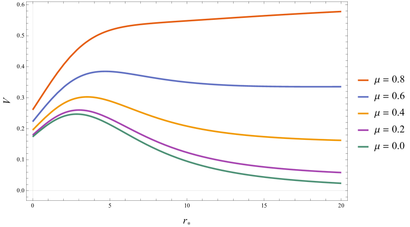
Figure 3: The ($n,\ell)=(0,2)$ mode of the scalar potential of Eq. (2.48) for increasing values of the parameter $\mu$. Note that for $\mu=0$, $V\rightarrow 0$ as $r_{*}\rightarrow\infty$ and the effective potential has a distinct peak. For $\mu\neq 0$, $V\rightarrow\mu^{2}$ as $r_{*}\rightarrow+\infty$. When $\mu^{2}\gtrsim V(r_{0})$, the peak is smoothed and the potential barrier is transformed into a potential step.

From Table 4 demonstrating the fundamental QNM mode, we observe that $\mathbb{R}e\{\omega\}$ increases steadily with $\mu$ whereas $\mathbb{I}m\{\omega\}$ decreases. As $\mu$ approaches $0.7$, there is a discernible change in the QNF behaviour: a large jump in both the real and imaginary parts is observed for all three methods, with a pronounced difference in the WKB result for $\mu=0.7$: a sudden drop in $\mathbb{R}e\{\omega\}$ and shift from negative to positive in $\mathbb{I}m\{\omega\}$. This represents a breakdown in the method: while there is a known increase in the relative error for $\mu=0.7$ Konoplya2019 , we observe explicitly from Fig. 3 that $\mu^{2}>V(r_{0})$ when $\mu=0.8$, which means the use of the WKB method is no longer appropriate.

However, there is also the physical interpretation to consider. In the geodesic picture, we understand that the flattening of the potential forbids the quantum tunnelling that allows the waves to “leak out” from the system. In Ref. Dolan2020_MassKerr , massive QNMs for which $\mathbb{R}e\{\omega^{2}\}>\mu^{2}$ are defined as “propagative” and behave similarly to their massless counterparts, whereas $\mathbb{R}e\{\omega^{2}\}<\mu^{2}$ are “evanescent” and contribute negligibly to the QNM spectrum for a perturbed black hole. This shift from propagative to evanescent is characterised by a change in sign in the imaginary part, as observed in Fig. 4. As $\mu$ increases, the QNMs transition from propagative to evanescent; as the imaginary part goes to zero, the QNMs enter the quasiresonance regime Ohashi2004_MassiveScalarQ , where the QNMs are arbitrarily long-lived. In this regime, the ingoing wave amplitude at the event horizon of the black hole is considered much smaller than the amplitude far from the black hole; since energy no longer “leaks” from the system at spatial infinity, the QNMs behave as standing waves Konoplya2004_MassiveScalar .

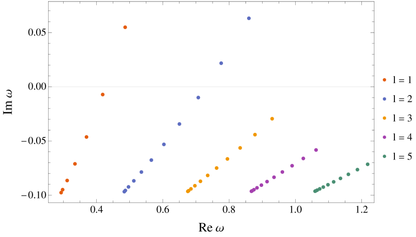
Figure 4: The QNF spectrum of the extra-dimensional scalar field whose higher-dimensional contribution emerges as a mass-like term. We use the Dolan-Ottewill method to plot the imaginary components against the real for $\mu\in\{0,1\}$. Note that even for these small multipolar numbers, the range of the QNF decreases for increasing $\ell$.

While we focus on the $\ell=2$ mode that dominates the observed QNF spectrum Berti2005_BHspectroscopy ; Carullo2019_pyRing1 , we can see in Fig. 4 that the oscillation timescale increases with the angular momentum number. This corresponds well to classical and quantum systems with which we are familiar, where the frequency of an oscillating wave increases with energy. Note, however, that as $\ell$ increases, the influence of $\mu$ wanes: the range of the QNF values converge to their massless counterpart for larger multipolar numbers.

In our extra-dimensional setup, the $\mu$ parameter serves as a manifestation of the extra dimensions, representing the KK tower of states. The analysis of the QNM potential and corresponding QNF spectrum conducted here demonstrates that only the “propagative” QNMs can be used as a probe in extra-dimensional searches. This places an upper bound on $\mu$, such that $\mathbb{R}e\{\omega^{2}\}>\mu^{2}$. For a scalar test field in the Schwarzschild black hole space-time, we therefore consider the bound from the numerical analysis to be $\mu\lesssim 0.6.$

3.3 An interpretation of $\mu$ in the QNM context

Within the QNM literature, potentials of the form provided in Eq. (2.48) have been approached primarily as a numerical problem (see e.g. Refs. SimoneWill1991_MassiveScalar ; Ohashi2004_MassiveScalarQ ; Konoplya2004_MassiveScalar ). However, a study of the $\mu$ parameter can also offer insights into the QNM problem at hand. To illustrate the role played by $\mu$ in QNM studies, and for a sense of the scales probed by QNFs influenced by this term, we discuss some examples from the literature.

Physically, we understand $\mu$ to be of dimensions of inverse length, such that $m=\mu\hbar$ (under units of $G=c=1$). The corresponding Compton wavelength $\lambda_{C}=h/(mc)$ can then be related to the mass in eV using

$$\lambda_{C}\times m=1.24\times 10^{-9}\;.$$ (3.52)

For Compton wavelengths corresponding to astrophysical black holes $m_{\mathrm{BH}}\sim 10M_{\odot}$, $\mu$ will correspond to very light particles of mass $m\sim 10^{-10}$ eV/c² Berti2014_BHprimer ; Lagos2020_Anomalous .

Motivated by the long-lived nature of massive scalar QNFs, an investigation into the gravitational perturbations coupled to the massive Klein-Gordon equation within a Schwarzschild space-time found similar masses, $m\sim 10^{-11}-10^{-12}$ eV/c² Herdeiro2014_MassiveFieldsBHs .

Of particular importance is the role played by the dimensionless parameter $M\mu$, where $M$ is the black hole Arnowitt-Deser-Misner (ADM) mass and $m=\mu\hbar$ as before is the bosonic field mass. In the case of spinning black holes, this dimensionless parameter acts as a scaling for the suppression of the instability timescale: when the Compton wavelength of the perturbing field is of the order of the black hole’s radius, the dimensionless parameter scales as $M\mu\sim 1$, leading to the strongest super-radiant instabilities for the Kerr black hole refBertiCardoso ; refKonoplyaZhidenkoReview . This scenario is applicable also to light primordial black holes Sasaki2018_PBHreview .

In a study of Proca field QNMs in the Kerr space-time Dolan2020_MassKerr , Dolan and Percival found $M\mu$ to be exceedingly large in the case of SM vector bosons, and extremely small for the photon with $\mu\lesssim 10^{-27}$ eV/c². Furthermore, they found that in the SM case, only evanescent modes for QNFs with $\ell+1/2\lesssim\mathcal{O}(M\mu)$ were predicted. For these extremely light photons, the QNF spectrum was anticipated to replicate that of the electromagnetic field, albeit with one extra longitudinal polarisation matching the QNF spectrum of a scalar field with mass $\mu>0$.

Since a number of BSM conjectures depend on the existence of light or even ultralight particles (e.g. light scalars of mass $10^{-32}\leq m\leq 10^{-10}$ eV as in the “string axiverse” scenarios Arvanitaki2009_StringAxiverse , dark or hidden photons, and other candidates PDG2022 ), massive QNMs may be useful in complementary searches for a variety of exotic signatures.

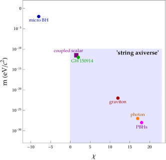
Figure 5: For a sense of the scales probed by QNFs for $M\mu\sim 1$, we illustrate the magnitudes of $m$ and $\chi$ of Eqs. (3.54) and (3.55) discussed in the text. We include the upper bounds for the photon mass Dolan2020_MassKerr and the graviton LIGO2021_GWTC3-GRtest , as well as the lower mass bound for massive primordial black holes Sasaki2018_PBHreview . We note that particles of these magnitudes correspond to those of the “string axiverse” scenarios Arvanitaki2009_StringAxiverse .

In our framework, we have positioned the $\mu$ parameter as an artefact of the extra-dimensional submanifold, representing the KK tower of states on the compact space. To obtain a sense of scale, we revert back to SI units such that the mass of the black hole and the $\mu$ parameter become

$$M=\frac{Gm^{\rm BH}}{c^{2}}\;\;\;\text{and}\;\;\;\mu=\frac{mc}{\hbar}\;.$$ (3.53)

From dimensional analysis, we can show that $M$ and $\mu$ have dimensions of length and inverse-length, respectively, such that $M\mu$ is indeed dimensionless. It is straightforward then that

$$M\mu = \frac{Gm^{\rm BH}m}{\hbar c}$$ (3.54)

$$\Rightarrow m=\frac{1}{m^{\rm BH}}\frac{\hbar c}{G}M\mu\;.$$

With the values $\hbar c/G\sim 10^{-16}$ kg², $1M_{\odot}\sim 10^{30}$ kg, and $M\mu\sim\mathcal{O}(1)$, we can scale the black hole mass as $m^{\rm BH}=10^{\chi}M_{\odot}$ and thereby express the extra-dimensional contribution through

$$m\sim 10^{-\chi}10^{-46}\text{kg}\sim 10^{-(\chi+10)}{\text{eV/c}}^{2}\;.$$ (3.55)

We may use this expression to explore possible mass limits. From the well-known mass limit for non-
evaporating primordial black holes $m_{\mathrm{PBH}}\gtrsim 10^{15}$ g Sasaki2018_PBHreview , $m\lesssim 10^{-28}\mathrm{eV/c^{2}}$ such that $\chi\gtrsim 18$. On the other hand, $\chi\sim-8$ corresponds to a micro black hole of the same mass as the moon. For the 62 $\pm\;4\;M_{\odot}$ black hole remnant corresponding to the GW150914 event refLIGO , $\chi\sim 2$.

We can also contrast this against the dynamical lower bound on the graviton Compton wavelength $\lambda_{g}\geq 10^{13}$ km, as determined by the LVK collaboration at a 90$\%$ confidence (using null tests against the modified dispersion relation of massive-graviton theory introduced in Ref. YunesWill2012_LorenzViolations ). This in turn corresponds to the upper bound on the graviton mass $m_{g}\lesssim 10^{-22}$ eV/c² LIGO2016_TestingGRGW150914 , which leads to the bound $\chi\gtrsim 12$.

4 Constraints from GWs using QNMs

In analogy to the electromagnetic waves produced by accelerating charges, GWs are generated by any massive body undergoing acceleration. This is a direct consequence of the relationship between mass and space-time curvature predicted by GR, where changes in the geometry occur corresponding to the movements of the massive body. Since gravity is weakly-interacting, the resultant ripples in space-time propagate throughout the universe unscreened. This property unlocks unique opportunities for studies into early-universe cosmology, since GWs decouple almost immediately after being produced and then propagate undisturbed throughout the universe; they may be the only way we can probe the time directly after the big bang Aggarwal2020_HighFGWs . However, a consequence of this feeble nature of gravity is a severely limited collection of astrophysical events whose corresponding GW signatures lie within the sensitivity range of detectors. These can be classified into four possible GW sources: coalescing compact bodies, pulsars, supernovae (all of which are sources of deterministic GWs), and a cosmic GW background comprised of the stochastic GWs emergent in the wake of the big bang Caldwell2022_GWLHCSnowMass ; Nature_GWreview .

The 90 GW events detected by the LVK collaboration refLIGO2018Run1 ; refLIGO2020Run2 ; refLIGO2021Run3a ; refLIGOrecentRun3b originate from the mergers of compact coalescing binaries, with binary black hole collisions remaining the most common. This is in part due to the energy output during a black hole collision (considered in Ref. refFerrari2008 as second only to the big bang), as well as the comprehensive understanding of the modelling of these two-body systems Jaranowski2005_GWanalysis . Three distinct phases make up the gravitational waveform (where parentheses indicate the technique through which each phase is modelled),

• inspiral: long, adiabatic stage as orbit shrinks and GW emission increases (post-Newtonian expansion);

• merger: violent merger into a single black hole and GW emission peaks (numerical relativity simulations);

• ringdown: final black hole emits damped GWs as it relaxes into a stationary state (black hole perturbation theory).

Due to the weakly-interacting nature of GWs and the noise in which the signal is saturated, inferring the physical parameters of a GW source is a delicate process dependent on prior knowledge of the expected signal shape and the implementation of several a priori assumptions (this is a highly non-trivial exercise, and we refer the interested reader to Ref. refLIGOguide for details). However, the observations of GWs from these merger events allow for unique tests of GR within regimes previously beyond reach.

In light of these regular GW detections and the promise of future GW observatories LIGO-India ; LISA ; CosmicExplorer , interest in using GW data to constrain BSM models is building (see Ref. Caldwell2022_GWLHCSnowMass ; Aggarwal2020_HighFGWs ). However, it is known that GW phenomenology is still in its infancy, unlike collider searches, where we have yet to obtain precise final state signatures for which we can search Yu2019 . This makes it difficult to constrain particle physics models with precision. Methods of searching for new physics predominantly rely on calculating the frequencies associated with symmetry breaking mechanisms to determine whether such signals lie within the sensitivity range of present or future GW detectors $-$ a strategy that long predates the detection of GWs Will1997_BoundGravitonCBC ; Hogan2000_GWsEDs1 ; Hogan2000_GWsEDs2 . Attempts to place bounds on the size and number of extra dimensions focus on the yet-undetected stochastic GW background rather than those emitted by compact coalescing bodies (see Ref. Yu2019 ).

Within the GW community, searches for modified theories of gravity consider how GW signals may differ from those of GR in terms of their generation, propagation, and polarisation LIGO2019_GWTC1-GRtest ; LIGO2020_GWTC2-GRtest_pyRing3 ; LIGO2021_GWTC3-GRtest . In the case of massive gravity theories, for example, it is well understood that additional polarisation states must be considered to describe the extra degrees of freedom. While GR has only two tensor modes (i.e. plus and cross modes), a generalised metric theory of gravity can accommodate up to six polarisation modes: two tensor, two vector, and two scalar modes Eardley1973_GWsExtraPolarisations ; deRham2017_GravitonMassBounds . Similar effects can be seen in extra-dimensional setups e.g. Ref. AndriotGomez2017_EDsignGWs ; in such cases, however, these can often lie far beyond detectable range Cardoso2019_GWsEDsKK ; Yu2019 . The situation is complicated further by the known difficulty in relating these null tests to one another Ghosh2022_RelatingGWtests .

For these reasons, we suggest a new avenue of pursuit by which to probe extra dimensions within extant GW data, that exploits the connection between QNM and GW studies. Inspired by tests for deviations from GR within the post-merger phase LIGO2020_GWTC2-GRtest_pyRing3 ; LIGO2021_GWTC3-GRtest , we make use of one of the few tools dedicated to QNM analyses of GW data: the Python package PyRing Carullo2019_pyRing1 ; refNoHair_pyRing2 . The package was recently developed to perform Bayesian parameter estimation, tests of GR, and other QNM analyses through a combination of observed GW data with simulation and numerically-generated waveform templates, following the Bayesian framework detailed in Ref. refLIGOguide . Treating GR as the null hypothesis, PyRing tests for deviations from the QNF oscillation frequency ($\mathbb{R}e\{\omega\}=\upomega$) and decay timescale ($1/\mathbb{I}m\{\omega\}=\tau$):

$$\delta\upomega = \upomega^{\rm GR}(1+\delta\upomega)\;,$$

$$\delta\tau = \tau^{\rm GR}(1+\delta\tau)\;.$$ (4.56)

Table 5: To correspond to the search for parametric deviations in GR, we structure our results for $\upomega=\mathbb{R}e\{\omega\}$ and the damping time $\tau=1/\mathbb{I}m\{\omega\}$ as $\upomega=\upomega^{\mu=0}\left(1+\delta\upomega\right)$ and $\tau=\tau^{\mu=0}\left(1+\delta\tau\right)$, respectively. We use QNF results provided in column 2 of Table 4.

$\mu$	$\omega(\ell,\mu)$	$\delta\upomega$	$\delta\tau$
$0.0$	$0.4836-0.0968i$	$0.0000$	$0.0000$
$0.1$	$0.4868-0.0968i$	$0.0065$	$0.0113$
$0.2$	$0.4963-0.0924i$	$0.0262$	$0.0473$
$0.3$	$0.5124-0.0868i$	$0.0594$	$0.1149$
$0.4$	$0.5352-0.0787i$	$0.1066$	$0.2302$
$0.5$	$0.5653-0.0676i$	$0.1687$	$0.4306$
$0.6$	$0.6032-0.0532i$	$0.2472$	$0.8206$
$\;0.7$	$\;\;0.6500-0.0343i$	$\;\;0.3440$	$1.8181$

As a first exploratory step, we run this agnostic test of GR deviation in GW data from the GW150914 black hole merger event refLIGO using the provided Kerr₂₂₀ waveform template corresponding to the $\ell=m=2$, $n=0$ mode (see Fig. 6). The analysis through PyRing is conducted in the time domain using publicly available data from the LVK collaboration LVK_OpenData . To reduce computational cost, we employ medium-resolution data, simplified noise estimation, and simplified sampler settings, as well as tight priors. Specifically, we follow Ref. Carullo2019_pyRing1 in sampling 4096s of data from the Hanford and the Livingston LIGO detectors, sampled at 4096 Hz with the raw strain band-passed over $f\in[20,2028]$ Hz before being split into 2-second noise chunks. We set the trigtime in H1 to $t=126259462.423227$ s. We run the analysis over prior bounds for final mass $M_{f}\leavevmode\nobreak\ \in\leavevmode\nobreak\ [50.0,90.0]\leavevmode\nobreak\ M_{\odot}$, spin $a_{f}\in[0.6,0.9]$, amplitude $A_{220}\in[0.0,5.0\times 10^{-20}]$, and phase $\phi_{220}\in[0,2\pi]$. In testing for deviations from GR, we sample over $\delta\upomega,\delta\tau\in[-1,1]$.

To carry out its Bayesian inference, PyRing exploits the nested sampling algorithm of cpnest Veitch_NestedSampling ; cpnest . The package’s implementation is based on an ensemble Markov chain Monte Carlo (MCMC) sampler, for which we only need to input the specifics of the analysis. We use 2048 live points and set the maximum MCMC steps to 2048, with the default 1234 seeds; at the end of the analysis, we are left with $\sim 8000$ independent samples. We visualise these results in Fig. 6.

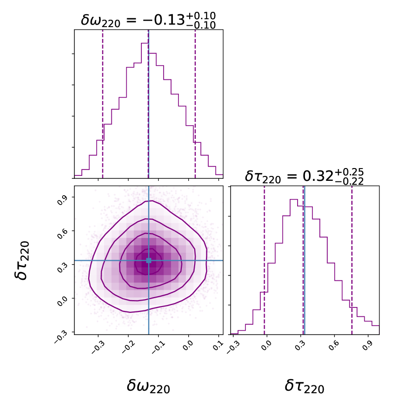
Figure 6: As a proof-of-concept, we perform a rudimentary parameter estimation of the GR deviations using PyRing for event GW150914 (GW data sampled at 4096 Hz). We narrow priors to reduce computation cost. With Corner, we plot the 2D posteriors and 1D histograms on ($\delta\omega$, $\delta\tau$), where $(0,0)$ is the GR-predicted value. Dashed lines and contours demarcate the 90% credible region; the blue line indicates the mean.

Higher resolution data diminishes the impact of the time discretisation Cotesta2022_OvertonesRingdown , while increased sampler settings lead to more precise results Veitch_NestedSampling ; cpnest . For improved accuracy, we therefore make use of the hierarchical combination of LVK’s strongest bounds on GR deviations to date LIGO2021_GWTC3-GRtest :

$$\delta\upomega_{220} = 0.02^{+0.07}_{-0.07}\;,$$

$$\delta\tau_{220} = 0.13^{+0.21}_{-0.22}\;.$$ (4.57)

To compare QNF computation with GW data, we consider our $\mu=0$ results to be equivalent to the GR prediction $(\delta\upomega,\delta\tau)=(0,0)$ i.e. $\upomega^{\mathrm{GR}}=\upomega^{\mu=0}$. From the Dolan-Ottewill results of Table 4, we extract the parametric deviations to Table 5. We observe that the parametric deviations match the bounds predicted in Eq. (4.57) for $\mu\sim 0.2$. If we exploit the QNF series expansion provided in Eq. (3.1), we can solve for $\mu$ explicitly. In doing so (for the real part and using the dominant $\ell=2,$ $n=0$ mode), we find that we can impose the upper bound

$$\mu\lesssim 0.3681\;.$$ (4.58)

This serves as an upper bound on the sensitivity of QNFs to extra-dimensional KK resonances, as construct- ed in this framework. Using Eq. (3.54), we can explore the physical insights that can be extracted from this limit.

Since we have set $M=1$, we can interpret this as a bound on the dimensionless parameter $M\mu$. As such, $M\mu\sim\mathcal{O}(0.1)$. Then for the final $M\sim 62M_{\odot}$ black hole remnant of GW150914, $\chi\sim 3$. This leads to the upper bound on the QNF probe,

$$m\lesssim 10^{-13}\mathrm{eV/c}^{2}\;.$$ (4.59)

In other words, we observe that applying static black hole QNFs as a direct probe into an agnostic extra-dimensional model demonstrates that QNFs cannot detect KK masses beyond roughly $m\sim 10^{-13}\mathrm{eV/c}^{2}$. We note that particles of this mass correspond to light scalar hypotheses rather than the TeV-scale KK masses of typical extra-dimensional conjectures PDG2022 .

5 Conclusions

In this work, we have considered a novel extra-dimen- sional setup comprised of a Schwarzschild black hole embedded in a 7D product space-time whose extra dimensions form a negative compact space $-$ specifically, a nilmanifold built from Heisenberg algebra. We have pursued a strategy for an extra-dimensional search using QNFs. By positioning the extra-dimensional contribution as an effective mass-like $\mu^{2}$ term in the QNM potential, we have demonstrated through a numerical study a possible upper bound on this $\mu$. For the scalar test-field and Schwarzschild space-time background considered here, $\mu\lesssim 0.6$.

Then, by using searches for parametric deviations from GR, we further constrain this probe to $\mu\lesssim 0.3681$. Via Eq. (3.54), we demonstrate that this corresponds to $m_{KK}\lesssim 10^{-13}\mathrm{eV/c}^{2}$. The limit provided in Eq. (4.58) can therefore be interpreted as a detectability bound on the QNM probe into extra dimensions. In other words, with currently available signals, we find that KK masses higher than roughly $m_{KK}\sim 10^{-13}\mathrm{eV/c^{2}}$ cannot be detected with QNMs.

However, there are a number of improvements that could be made to this preliminary study that may lead to more stringent bounds, particularly in the application to other BSM scenarios. For example, we would expect minor corrections from the use of the more astro- physically-relevant Kerr black hole space-time and gravitational QNFs; this would be necessary for greater precision than the order-of-magnitude study conducted in this work. More significantly, we recognise that this investigation was limited by the need to adopt an agnostic approach to our pursuit of evidence of extra dimensions. As the LVK collaboration develops more sophisticated and model-specific ringdown templates to test for parametric deviations in GR, it would be interesting to observe how theoretical frameworks can be adapted to the question of searches for extra-dimensional signatures in GWs.

A further open question is to what extent can we apply such constraints to place bounds on the size and number of extra dimensions. For example, a next step for this study could be to subject the mass spectrum of the toy dark matter model studied in Ref. Andriot2016_TowardsKK to this result in order to extract tangible bounds on the radius of the nilmanifold extra dimensions herein constructed. Moreover, a detailed investigation of the propagation of GWs in nilmanifold spaces is reserved for a future work.

As acknowledged in Ref. LIGO2021_GWTC3-GRtest , there has been substantial progress in GW research from the analytical, numerical, and experimental fronts. GW phenomenology and our ability to perform precision-level testing of GR, however, are still in their infancy. It is our hope that the simple setup we have provided here may be refined as our understanding of the applicability of GW detection in fundamental physics grows, bringing these tests to a new level of accuracy.

- (1) C.V. Vishveshwara, Nature 227, 936 (1970). DOI 10.1038/227936a0
- (2) W.H. Press, Astrophys. J. Lett. 170, L105 (1971). DOI 10.1086/180849
- (3) H.P. Nollert, Class. Quant. Grav. 16, R159 (1999). DOI 10.1088/0264-9381/16/12/201
- (4) K.D. Kokkotas, B.G. Schmidt, Living Rev. Rel. 2, 2 (1999). DOI 10.12942/lrr-1999-2
- (5) V. Ferrari, L. Gualtieri, Gen. Rel. Grav. 40, 945 (2008). DOI 10.1007/s10714-007-0585-1
- (6) E. Berti, V. Cardoso, A.O. Starinets, Class. Quant. Grav. 26, 163001 (2009). DOI 10.1088/0264-9381/26/16/163001
- (7) R.A. Konoplya, A. Zhidenko, Rev. Mod. Phys. 83, 793 (2011). DOI 10.1103/RevModPhys.83.793
- (8) F. Echeverria, Phys. Rev. D 40, 3194 (1989). DOI 10.1103/PhysRevD.40.3194. URL https://link.aps.org/doi/10.1103/PhysRevD.40.3194
- (9) C.W. Misner, K.S. Thorne, J.A. Wheeler, Gravitation (W. H. Freeman, San Francisco, 1973)
- (10) I.H. Stairs, Living Rev. Rel. 6, 5 (2003). DOI 10.12942/lrr-2003-5
- (11) D. Merritt, T. Alexander, S. Mikkola, C.M. Will, Phys. Rev. D 81, 062002 (2010). DOI 10.1103/PhysRevD.81.062002
- (12) C.M. Will, Living Rev. Rel. 17(1), 4 (2014). DOI 10.12942/lrr-2014-4. URL https://doi.org/10.12942/lrr-2014-4
- (13) E. Berti, et al., Class. Quant. Grav. 32, 243001 (2015). DOI 10.1088/0264-9381/32/24/243001
- (14) W. Israel, Phys. Rev. 164, 1776 (1967). DOI 10.1103/PhysRev.164.1776. URL https://link.aps.org/doi/10.1103/PhysRev.164.1776
- (15) T. Regge, J.A. Wheeler, Phys. Rev. 108, 1063 (1957). DOI 10.1103/PhysRev.108.1063
- (16) F.J. Zerilli, Phys. Rev. D 2, 2141 (1970). DOI 10.1103/PhysRevD.2.2141
- (17) M. Davis, R. Ruffini, W.H. Press, R.H. Price, Phys. Rev. Lett. 27, 1466 (1971). DOI 10.1103/PhysRevLett.27.1466
- (18) C. Gundlach, R.H. Price, J. Pullin, Phys. Rev. D 49, 883 (1994). DOI 10.1103/PhysRevD.49.883
- (19) E.W. Leaver, Proc. Roy. Soc. Lond. A 402, 285 (1985). DOI 10.1098/rspa.1985.0119
- (20) O.J.C. Dias, P. Figueras, R. Monteiro, J.E. Santos, R. Emparan, Phys. Rev. D 80, 111701 (2009). DOI 10.1103/PhysRevD.80.111701
- (21) O.J.C. Dias, P. Figueras, R. Monteiro, H.S. Reall, J.E. Santos, JHEP 05, 076 (2010). DOI 10.1007/JHEP05(2010)076
- (22) H. Ciftci, R.L. Hall, N. Saad, J. Phys. A. Math. Gen. 36(47), 11807 (2003). DOI 10.1088/0305-4470/36/47/008
- (23) H.T. Cho, A.S. Cornell, J. Doukas, W. Naylor, Class. Quant. Grav. 27, 155004 (2010). DOI 10.1088/0264-9381/27/15/155004
- (24) G.T. Horowitz, V.E. Hubeny, Phys. Rev. D 62, 024027 (2000). DOI 10.1103/PhysRevD.62.024027
- (25) G. Pöschl, E. Teller, Z. Phys. 83, 143 (1933). DOI 10.1007/BF01331132
- (26) H.J. Blome, B. Mashhoon, Physics Letters A 100(5), 231 (1984). DOI https://doi.org/10.1016/0375-9601(84)90769-2. URL https://www.sciencedirect.com/science/article/pii/0375960184907692
- (27) B.F. Schutz, C.M. Will, Astrophys. J. 291, L33 (1985). DOI 10.1086/184453
- (28) C.M. Will, Can. J. Phys. 64(2), 140 (1986). DOI 10.1139/p86-023
- (29) S. Iyer, C.M. Will, Phys. Rev. D 35(12), 3621 (1987). DOI 10.1103/PhysRevD.35.3621
- (30) R.A. Konoplya, Phys. Rev. D 68, 024018 (2003). DOI 10.1103/PhysRevD.68.024018
- (31) R.A. Konoplya, A. Zhidenko, A.F. Zinhailo, Class. Quant. Grav. 36, 155002 (2019). DOI 10.1088/1361-6382/ab2e25
- (32) S.R. Dolan, A.C. Ottewill, Class. Quant. Grav. 26, 225003 (2009). DOI 10.1088/0264-9381/26/22/225003
- (33) C.J. Goebel, Astrophys. J. 172(L95) (1972)
- (34) C.H. Chen, H.T. Cho, A. Chrysostomou, A.S. Cornell, Phys. Rev. D 104(2), 024009 (2021). DOI 10.1103/PhysRevD.104.024009
- (35) P. Grandclement, J. Novak, Living Rev. Rel. 12, 1 (2009). DOI 10.12942/lrr-2009-1
- (36) O.J.C. Dias, J.E. Santos, B. Way, Class. Quant. Grav. 33(13), 133001 (2016). DOI 10.1088/0264-9381/33/13/133001
- (37) B.P. Abbott, et al., Phys. Rev. X 9(3), 031040 (2019). DOI 10.1103/PhysRevX.9.031040
- (38) R. Abbott, et al., Phys. Rev. X 11, 021053 (2021). DOI 10.1103/PhysRevX.11.021053
- (39) R. Abbott, et al., (2021)
- (40) R. Abbott, et al., (2021)
- (41) R. Abbott, et al., (2021)
- (42) N. Yunes, K. Yagi, F. Pretorius, Phys. Rev. D 94(8), 084002 (2016). DOI 10.1103/PhysRevD.94.084002
- (43) L. Barack, et al., Class. Quant. Grav. 36(14), 143001 (2019). DOI 10.1088/1361-6382/ab0587
- (44) D.J. Weir, Phil. Trans. Roy. Soc. Lond. A 376(2114), 20170126 (2018). DOI 10.1098/rsta.2017.0126
- (45) R.G. Cai, Z. Cao, Z.K. Guo, S.J. Wang, T. Yang, National Science Review 4(5), 687 (2017). DOI 10.1093/nsr/nwx029. URL https://doi.org/10.1093/nsr/nwx029
- (46) M. Bailes, et al., Nature Rev. Phys. 3(5), 344 (2021). DOI 10.1038/s42254-021-00303-8
- (47) N. Aggarwal, et al., Living Rev. Rel. 24(1), 4 (2021). DOI 10.1007/s41114-021-00032-5
- (48) A. Alves, T. Ghosh, H.K. Guo, K. Sinha, D. Vagie, JHEP 04, 052 (2019). DOI 10.1007/JHEP04(2019)052
- (49) R. Caldwell, et al., Gen. Rel. Grav. 54(12), 156 (2022). DOI 10.1007/s10714-022-03027-x
- (50) W.C. Huang, F. Sannino, Z.W. Wang, Phys. Rev. D 102(9), 095025 (2020). DOI 10.1103/PhysRevD.102.095025
- (51) C.J. Moore, R.H. Cole, C.P.L. Berry, Class. Quant. Gravity 32(1), 015014 (2014). DOI 10.1088/0264-9381/32/1/015014. URL http://dx.doi.org/10.1088/0264-9381/32/1/015014
- (52) S. Chigusa, Y. Nakai, J. Zheng, Phys. Rev. D 104(3), 035031 (2021). DOI 10.1103/PhysRevD.104.035031
- (53) S.F. King, S. Pascoli, J. Turner, Y.L. Zhou, JHEP 10, 225 (2021). DOI 10.1007/JHEP10(2021)225
- (54) J.A. Dror, T. Hiramatsu, K. Kohri, H. Murayama, G. White, Phys. Rev. Lett. 124(4), 041804 (2020). DOI 10.1103/PhysRevLett.124.041804
- (55) W. Buchmuller, V. Domcke, H. Murayama, K. Schmitz, Phys. Lett. B 809, 135764 (2020). DOI 10.1016/j.physletb.2020.135764
- (56) H. Yu, Z.C. Lin, Y.X. Liu, Commun. Theor. Phys. 71(8), 991 (2019). DOI 10.1088/0253-6102/71/8/991
- (57) V. Cardoso, L. Gualtieri, C.J. Moore, Phys. Rev. D 100(12), 124037 (2019). DOI 10.1103/PhysRevD.100.124037
- (58) O.K. Kwon, S. Lee, D.D. Tolla, Phys. Rev. D 100, 084050 (2019). DOI 10.1103/PhysRevD.100.084050
- (59) D. Andriot, G. Lucena Gómez, JCAP 06, 048 (2017). DOI 10.1088/1475-7516/2017/06/048. [Erratum: JCAP 05, E01 (2019)]
- (60) Y. Du, S. Tahura, D. Vaman, K. Yagi, Phys. Rev. D 103, 044031 (2021). DOI 10.1103/PhysRevD.103.044031. URL https://link.aps.org/doi/10.1103/PhysRevD.103.044031
- (61) C. Ferko, G. Satishchandran, S. Sethi, Phys. Rev. D 105, 024072 (2022). DOI 10.1103/PhysRevD.105.024072
- (62) D. Andriot, D. Tsimpis, JHEP 06, 100 (2020). DOI 10.1007/JHEP06(2020)100
- (63) D. Andriot, P. Marconnet, D. Tsimpis, JCAP 07, 040 (2021). DOI 10.1088/1475-7516/2021/07/040
- (64) E. Berti, V. Cardoso, J.A. Gonzalez, U. Sperhake, M. Hannam, S. Husa, B. Bruegmann, Phys. Rev. D 76, 064034 (2007). DOI 10.1103/PhysRevD.76.064034
- (65) C. Van Den Broeck, A. Ashtekar, V. Petkov, Probing dynamical spacetimes with gravitational waves (Springer, 2014), pp. 589–613. DOI 10.1007/978-3-642-41992-8˙27
- (66) B.P. Abbott, et al., Class. Quant. Grav. 37(5), 055002 (2020). DOI 10.1088/1361-6382/ab685e
- (67) B.P. Abbott, et al., Phys. Rev. D 100(10), 104036 (2019). DOI 10.1103/PhysRevD.100.104036
- (68) R. Abbott, et al., Phys. Rev. D 103(12), 122002 (2021). DOI 10.1103/PhysRevD.103.122002
- (69) R. Abbott, et al., (2021)
- (70) B.P. Abbott, et al., Phys. Rev. Lett. 116(6), 061102 (2016). DOI 10.1103/PhysRevLett.116.061102
- (71) B.P. Abbott, et al., Phys. Rev. Lett. 116(24), 241102 (2016). DOI 10.1103/PhysRevLett.116.241102
- (72) B.P. Abbott, et al., Phys. Rev. Lett. 116(22), 221101 (2016). DOI 10.1103/PhysRevLett.116.221101. [Erratum: Phys.Rev.Lett. 121, 129902 (2018)]
- (73) V. Baibhav, E. Berti, V. Cardoso, Phys. Rev. D 101(8), 084053 (2020). DOI 10.1103/PhysRevD.101.084053
- (74) I. Ota, C. Chirenti, Phys. Rev. D 105(4), 044015 (2022). DOI 10.1103/PhysRevD.105.044015
- (75) S. Bhagwat, C. Pacilio, E. Barausse, P. Pani, (2021)
- (76) E. Berti, V. Cardoso, C.M. Will, Phys. Rev. D 73, 064030 (2006). DOI 10.1103/PhysRevD.73.064030
- (77) G. Carullo, W. Del Pozzo, J. Veitch, Phys. Rev. D 99(12), 123029 (2019). DOI 10.1103/PhysRevD.99.123029. [Erratum: Phys.Rev.D 100, 089903 (2019)]
- (78) C.D. Capano, M. Cabero, J. Westerweck, J. Abedi, S. Kastha, A.H. Nitz, A.B. Nielsen, B. Krishnan, (2021)
- (79) R. Cotesta, G. Carullo, E. Berti, V. Cardoso, Phys. Rev. Lett. 129(11), 111102 (2022). DOI 10.1103/PhysRevLett.129.111102
- (80) G. Carullo, et al., Phys. Rev. D 98(10), 104020 (2018). DOI 10.1103/PhysRevD.98.104020
- (81) R. Cotesta, G. Carullo, E. Berti, V. Cardoso, Phys. Rev. Lett. 129(11), 111102 (2022). DOI 10.1103/PhysRevLett.129.111102
- (82) M. Isi, M. Giesler, W.M. Farr, M.A. Scheel, S.A. Teukolsky, Phys. Rev. Lett. 123(11), 111102 (2019). DOI 10.1103/PhysRevLett.123.111102
- (83) M. Isi, W.M. Farr, (2022)
- (84) A. Ghosh, R. Brito, A. Buonanno, Phys. Rev. D 103(12), 124041 (2021). DOI 10.1103/PhysRevD.103.124041
- (85) L. Randall, R. Sundrum, Phys. Rev. Lett. 83, 4690 (1999). DOI 10.1103/PhysRevLett.83.4690
- (86) T. Shiromizu, K.i. Maeda, M. Sasaki, Phys. Rev. D 62, 024012 (2000). DOI 10.1103/PhysRevD.62.024012
- (87) A.K. Mishra, A. Ghosh, S. Chakraborty, Eur. Phys. J. C 82(9), 820 (2022). DOI 10.1140/epjc/s10052-022-10788-x
- (88) D. Andriot, G. Cacciapaglia, A. Deandrea, N. Deutschmann, D. Tsimpis, JHEP 06, 169 (2016). DOI 10.1007/JHEP06(2016)169
- (89) T. Needham, Visual complex analysis (Clarendon Press, 2012)
- (90) M. Berger, A Panoramic View of Riemannian Geometry (Springer Berlin, 2013)
- (91) S.S. Haque, G. Shiu, B. Underwood, T. Van Riet, Phys. Rev. D 79, 086005 (2009). DOI 10.1103/PhysRevD.79.086005
- (92) D. Andriot, J. Blåbäck, JHEP 03, 102 (2017). DOI 10.1007/JHEP03(2017)102. [Erratum: JHEP 03, 083 (2018)]
- (93) D. Andriot, L. Horer, P. Marconnet, JHEP 06, 131 (2022). DOI 10.1007/JHEP06(2022)131
- (94) G.D. Starkman, D. Stojkovic, M. Trodden, Phys. Rev. Lett. 87, 231303 (2001). DOI 10.1103/PhysRevLett.87.231303
- (95) C.M. Chen, P.M. Ho, I.P. Neupane, N. Ohta, J.E. Wang, JHEP 10, 058 (2003). DOI 10.1088/1126-6708/2003/10/058
- (96) I.P. Neupane, Class. Quant. Grav. 21, 4383 (2004). DOI 10.1088/0264-9381/21/18/007
- (97) D. Orlando, S.C. Park, JHEP 08, 006 (2010). DOI 10.1007/JHEP08(2010)006
- (98) L. Randall, R. Sundrum, Phys. Rev. Lett. 83, 3370 (1999). DOI 10.1103/PhysRevLett.83.3370
- (99) D. Andriot, D. Tsimpis, JHEP 09, 096 (2018). DOI 10.1007/JHEP09(2018)096
- (100) D. Andriot, A. Cornell, A. Deandrea, F. Dogliotti, D. Tsimpis, JHEP 05, 122 (2020). DOI 10.1007/JHEP05(2020)122
- (101) A. Deandrea, F. Dogliotti, D. Tsimpis, Phys. Lett. B 829, 137097 (2022). DOI 10.1016/j.physletb.2022.137097
- (102) A. Deandrea, F. Dogliotti, D. Tsimpis, Nucl. Phys. B 982, 115895 (2022). DOI 10.1016/j.nuclphysb.2022.115895
- (103) D. Andriot, JHEP 02, 112 (2016). DOI 10.1007/JHEP02(2016)112
- (104) C. Bock, Asian Journal of Mathematics 20(2), 199 (2016)
- (105) M. Grana, R. Minasian, M. Petrini, A. Tomasiello, JHEP 05, 031 (2007). DOI 10.1088/1126-6708/2007/05/031
- (106) D. Andriot, String theory flux vacua on twisted tori and Generalized Complex Geometry. Ph.D. thesis, Paris U., VI-VII (2010)
- (107) A.I. Malcev, Amer. Math. Soc. Translation 39 (1951)
- (108) S. Thangavelu, Revista de la Union Matematica Argentina 50, 71 (2009)
- (109) J.D. Bekenstein, Contemp. Phys. 45, 31 (2003). DOI 10.1080/00107510310001632523
- (110) S. Chandrasekhar, The Mathematical Theory of Black Holes (Oxford Univerity Press, New York, 1983)
- (111) S.W. Hawking, Commun. Math. Phys. 43, 199 (1975). DOI 10.1007/BF02345020. [Erratum: Commun.Math.Phys. 46, 206 (1976)]
- (112) W. Barreto, A. Da Silva, R. Gomez, L. Lehner, L. Rosales, J. Winicour, Phys. Rev. D 71, 064028 (2005). DOI 10.1103/PhysRevD.71.064028
- (113) H. Yoshino, T. Shiromizu, M. Shibata, Phys. Rev. D 74, 124022 (2006). DOI 10.1103/PhysRevD.74.124022
- (114) L.E. Simone, C.M. Will, Class. Quant. Grav. 9, 963 (1992). DOI 10.1088/0264-9381/9/4/012
- (115) A. Ohashi, M.a. Sakagami, Class. Quant. Grav. 21, 3973 (2004). DOI 10.1088/0264-9381/21/16/010
- (116) R.A. Konoplya, A.V. Zhidenko, Phys. Lett. B 609, 377 (2005). DOI 10.1016/j.physletb.2005.01.078
- (117) S.R. Dolan, Phys. Rev. D 76, 084001 (2007). DOI 10.1103/PhysRevD.76.084001
- (118) J.G. Rosa, S.R. Dolan, Phys. Rev. D 85, 044043 (2012). DOI 10.1103/PhysRevD.85.044043
- (119) B.C. Seymour, K. Yagi, Classical and Quantum Gravity 37(14), 145008 (2020). DOI 10.1088/1361-6382/ab9933. URL https://doi.org/10.1088/1361-6382/ab9933
- (120) V. Ferrari, B. Mashhoon, Phys. Rev. D 30, 295 (1984). DOI 10.1103/PhysRevD.30.295
- (121) V. Ferrari, B. Mashhoon, Phys. Rev. Lett. 52(16), 1361 (1984). DOI 10.1103/PhysRevLett.52.1361
- (122) N. Fröman, P.O. Fröman, JWKB Approximation: Contributions to the Theory, 1st edn. (North-Holland, Amsterdam, 1965)
- (123) J. Percival, S.R. Dolan, Phys. Rev. D 102(10), 104055 (2020). DOI 10.1103/PhysRevD.102.104055
- (124) J. Matyjasek, M. Opala, Phys. Rev. D 96(2), 024011 (2017). DOI 10.1103/PhysRevD.96.024011
- (125) J. Matyjasek, M. Telecka, Phys. Rev. D 100(12), 124006 (2019). DOI 10.1103/PhysRevD.100.124006
- (126) A. Zhidenko, Class. Quantum Gravity 21(1), 273 (2004). DOI 10.1088/0264-9381/21/1/019
- (127) E. Berti, in DPG Physics School ”General Relativity @ 99” (2014)
- (128) M. Lagos, P.G. Ferreira, O.J. Tattersall, Phys. Rev. D 101(8), 084018 (2020). DOI 10.1103/PhysRevD.101.084018
- (129) J.C. Degollado, C.A.R. Herdeiro, Phys. Rev. D 90(6), 065019 (2014). DOI 10.1103/PhysRevD.90.065019
- (130) M. Sasaki, T. Suyama, T. Tanaka, S. Yokoyama, Class. Quant. Grav. 35(6), 063001 (2018). DOI 10.1088/1361-6382/aaa7b4
- (131) A. Arvanitaki, S. Dimopoulos, S. Dubovsky, N. Kaloper, J. March-Russell, Phys. Rev. D 81, 123530 (2010). DOI 10.1103/PhysRevD.81.123530
- (132) R.L. Workman, Others, PTEP 2022, 083C01 (2022). DOI 10.1093/ptep/ptac097
- (133) S. Mirshekari, N. Yunes, C.M. Will, Phys. Rev. D 85, 024041 (2012). DOI 10.1103/PhysRevD.85.024041
- (134) P. Jaranowski, A. Krolak, Living Rev. Rel. 8, 3 (2005)
- (135) C.S. Unnikrishnan, Int. J. Mod. Phys. D 22, 1341010 (2013). DOI 10.1142/S0218271813410101
- (136) P. Amaro-Seoane, et al., Class. Quant. Grav. 29, 124016 (2012). DOI 10.1088/0264-9381/29/12/124016
- (137) D. Reitze, et al., Bull. Am. Astron. Soc. 51(7), 035 (2019)
- (138) C.M. Will, Phys. Rev. D 57, 2061 (1998). DOI 10.1103/PhysRevD.57.2061
- (139) C.J. Hogan, Phys. Rev. Lett. 85, 2044 (2000). DOI 10.1103/PhysRevLett.85.2044. URL https://link.aps.org/doi/10.1103/PhysRevLett.85.2044
- (140) C.J. Hogan, Phys. Rev. D 62, 121302 (2000). DOI 10.1103/PhysRevD.62.121302
- (141) D.M. Eardley, D.L. Lee, A.P. Lightman, R.V. Wagoner, C.M. Will, Phys. Rev. Lett. 30, 884 (1973). DOI 10.1103/PhysRevLett.30.884. URL https://link.aps.org/doi/10.1103/PhysRevLett.30.884
- (142) C. de Rham, J.T. Deskins, A.J. Tolley, S.Y. Zhou, Rev. Mod. Phys. 89(2), 025004 (2017). DOI 10.1103/RevModPhys.89.025004
- (143) N.K. Johnson-McDaniel, A. Ghosh, S. Ghonge, M. Saleem, N.V. Krishnendu, J.A. Clark, Phys. Rev. D 105(4), 044020 (2022). DOI 10.1103/PhysRevD.105.044020
- (144) R. Abbott, et al., SoftwareX 13, 100658 (2021). DOI 10.1016/j.softx.2021.100658
- (145) J. Veitch, A. Vecchio, Phys. Rev. D 81, 062003 (2010). DOI 10.1103/PhysRevD.81.062003
- (146) J. Veitch, W.D. Pozzo, A. Lyttle, M.J. Williams, C. Talbot, M. Pitkin, G. Ashton, Cody, M. Hübner, A. Nitz, D. Mihaylov, D. Macleod, G. Carullo, G. Davies, ttw. johnveitch/cpnest: v0.11.4 (2022). DOI 10.5281/zenodo.6460935. URL https://doi.org/10.5281/zenodo.6460935
- (147) D. Foreman-Mackey, The Journal of Open Source Software 1(2), 24 (2016). DOI 10.21105/joss.00024. URL https://doi.org/10.21105/joss.00024
- (148) S. Behnel, R. Bradshaw, C. Citro, L. Dalcin, D.S. Seljebotn, K. Smith, Computing in Science & Engineering 13(2), 31 (2011)
- (149) A. Collette, Python and HDF5 (O’Reilly, 2013)
- (150) J.D. Hunter, Computing in Science & Engineering 9(3), 90 (2007). DOI 10.1109/MCSE.2007.55
- (151) C.R. Harris, K.J. Millman, S.J. van der Walt, R. Gommers, P. Virtanen, D. Cournapeau, E. Wieser, J. Taylor, S. Berg, N.J. Smith, R. Kern, M. Picus, S. Hoyer, M.H. van Kerkwijk, M. Brett, A. Haldane, J.F. del Río, M. Wiebe, P. Peterson, P. Gérard-Marchant, K. Sheppard, T. Reddy, W. Weckesser, H. Abbasi, C. Gohlke, T.E. Oliphant, Nature 585(7825), 357 (2020). DOI 10.1038/s41586-020-2649-2. URL https://doi.org/10.1038/s41586-020-2649-2
- (152) P. Virtanen, R. Gommers, T.E. Oliphant, M. Haberland, T. Reddy, D. Cournapeau, E. Burovski, P. Peterson, W. Weckesser, J. Bright, S.J. van der Walt, M. Brett, J. Wilson, K.J. Millman, N. Mayorov, A.R.J. Nelson, E. Jones, R. Kern, E. Larson, C.J. Carey, İ. Polat, Y. Feng, E.W. Moore, J. VanderPlas, D. Laxalde, J. Perktold, R. Cimrman, I. Henriksen, E.A. Quintero, C.R. Harris, A.M. Archibald, A.H. Ribeiro, F. Pedregosa, P. van Mulbregt, SciPy 1.0 Contributors, Nature Methods 17, 261 (2020). DOI 10.1038/s41592-019-0686-2
- (153) M.L. Waskom, Journal of Open Source Software 6(60), 3021 (2021). DOI 10.21105/joss.03021. URL https://doi.org/10.21105/joss.03021