Microscopic dynamics at the Running of the Bulls (San Fermín Festival) in the context of the Social Force Model

Abstract

This research explores the dynamics of the emergency evacuation during the “Running of the Bulls” festival (Spain, 2013). As people run to escape from danger, many pedestrians stumble and fall down, while others will try to pass over them. We carefully examined three specific recordings of the running, that show this kind of behavior. We developed a microscopic model mimicking the stumbling mechanism in the context of the Social Force Model (SFM). In our model, “moving” individuals can suddenly switch to a “fallen” state when they are in the vicinity of a fallen individual. We arrived to the conclusion that the presence of a fallen pedestrian increases dramatically the falling probability of the pedestrians nearby. Also, the product between the local density gradient and the velocity of each pedestrian appears as a relevant indicator for an imminent fall. We call this the pedestrian “falling susceptibility ($f_{s}$)”.

1 Introduction

The matter of emergency evacuation is of obvious importance in common life. In the last decades, a growing interest appeared in the research of the pedestrian dynamics during an emergency evacuation. The proper understanding of the evacuation dynamics will allow safer facilities when designing common spaces.

The evacuation through narrow pathways or doorways appears as one of the most studied scenarios in the literature. Many experiments and numerical simulations have been carried out for a better understanding of the crowd behavior in a variety of situations. These investigations focus on the door width as the main cause of the overcrowding during the evacuation process [1, 2, 3, 4, 5, 6, 7, 8, 9]. Therefore, it is pointed as the key magnitude affecting the evacuation performance.

The dynamic of emergency evacuations through narrow doors is dominated by “blockings”. Research has shown that a small group of pedestrians close to the door can be responsible for blocking the way to the rest of the crowd by forming an arch-like metastable structure, or blocking cluster, yielding long lasting delays [10, 11, 12, 13]. Also, the pressure inside the bulk is considered to be of decisive importance in the breaking process of the blocking clusters [14, 10, 12, 13, 15, 16, 17, 18, 19, 20].

The pedestrian’s anxiety [13], the presence of obstacles [21] and the possibility of fallings [22] are all relevant issues that affect the formation of blocking clusters in the context of narrow doors (bottlenecks). However, blocking clusters are expected to become irrelevant out of this context [10], and therefore, the connection between the aforementioned issues and the evacuation performance appears somehow obscure.

The emergency evacuations in the absence of blocking clusters are, from our point of view, an unattended matter throughout the literature. Thus, we decided to place the attention on those situations where the blocking clusters are quite improbable (i.e. wide openings), but fallings are still a relevant issue. Specifically, our investigation focuses on three real-life situations (empirical approach) of the “Running of the Bulls” event (2013). The videos capture the instances where participants stumble and fall during the rush in different wide door scenarios [23, 24, 25].

Our first objective is to acquire reliable data from real stumbling events, and use this data to build a formalism to recognize situations in which tripping becomes highly probable within the context of the SFM. We assume that pedestrians behave as either “moving” or “fallen” individuals. The transition probabilities from the “moving” behavior to the “fallen” one corresponds to those from the video recordings. No transition from “fallen” to “moving” is permitted under this approach.

We emphasize the critical attitude that we sustained along the investigation. Our SFM model was tested before proceeding to other hypothetical scenarios. Results showed fairly good agreement with the analyzed videos.

The investigation is organized as follows. A brief review of the basic “Social Force Model” can be found in Section 2. In Section 3 we present the real-life situations considered in our investigation, while in Section 4 we provide details on the numerical simulations. Section 5 present the results from both the empirical and numerical analyses. The corresponding conclusions are summarized in Section 6.

2 Background

2.1 The social force model

This investigation handles the pedestrians dynamics in the context of the “Social Force Model” (SFM) [14]. The SFM exploits the idea that human motion depends on the people’s own desire to reach a certain destination at a given velocity, as well as other environmental factors [26]. The former is modeled by a force called the “desire force”, while the latter is represented by “social forces” and “granular forces”. These forces enter the equation of motion as follows

$$m_{i}\,\displaystyle\frac{d\mathbf{v}^{(i)}}{dt}=\mathbf{f}_{d}^{(i)}+\displaystyle\sum_{j=1}^{N}\displaystyle\mathbf{f}_{s}^{(ij)}+\displaystyle\sum_{j=1}^{N}\mathbf{f}_{g}^{(ij)}$$ (1)

where the $i,j$ subscripts correspond to any two pedestrians in the crowd. $\mathbf{v}^{(i)}(t)$ means the current velocity of the pedestrian $(i)$, while $\mathbf{f}_{d}$ and $\mathbf{f}_{s}$ correspond to the “desired force” and the “social force”, respectively. $\mathbf{f}_{g}$ is the friction or granular force.

The $\mathbf{f}_{d}$ describes the pedestrians own desire to reach a specific target position at the desired velocity $v_{d}$. But, due to environmental factors (i.e. obstacles, visibility), he (she) actually moves at the current velocity $\mathbf{v}^{(i)}(t)$. Thus, he (she) will accelerate (or decelerate) to reach any desired velocity $v_{d}$ that will make him (her) feel more comfortable. Thus, in the Social Force Model, the desired force reads [14]

$$\mathbf{f}_{d}^{(i)}(t)=m_{i}\,\displaystyle\frac{v_{d}^{(i)}\,\mathbf{e}_{d}^{(i)}(t)-\mathbf{v}^{(i)}(t)}{\tau}$$ (2)

where $m_{i}$ is the mass of the pedestrian $i$ and $\tau$ represents the relaxation time needed to reach the desired velocity. $\mathbf{e}_{d}$ is the unit vector pointing to the target position. Detailed values for $m_{i}$ and $\tau$ can be found in Refs. [14, 21, 27, 28].

The “social force” $\mathbf{f}_{s}(t)$ represents the socio-psychological tendency of the pedestrians to preserve their private sphere. The spatial preservation means that a repulsive feeling exists between two neighboring pedestrians, or, between the pedestrian and the walls [14, 26]. This repulsive feeling becomes stronger as people get closer to each other (or to the walls). Thus, in the context of the Social Force Model, this tendency is expressed as

$$\mathbf{f}_{s}^{(ij)}=A_{i}\,e^{(r_{ij}-d_{ij})/B_{i}}\mathbf{n}_{ij}$$ (3)

where $(ij)$ corresponds to any two pedestrians, or to the pedestrian-wall interaction. $A_{i}$ and $B_{i}$ are two fixed parameters (see Ref. [10]). The distance $r_{ij}=r_{i}+r_{j}$ is the sum of the pedestrians radius, while $d_{ij}$ is the distance between the center of mass of the pedestrians $i$ and $j$. $\mathbf{n}_{ij}$ means the unit vector in the $\vec{ji}$ direction. For the case of repulsive feelings with the walls, $d_{ij}$ corresponds to the shortest distance between the pedestrian and the wall, while $r_{ij}=r_{i}$ (see Refs. [14, 26]).

It is worth mentioning that the Eq. (3) is also valid if two pedestrians are in contact (i.e. $r_{ij}>d_{ij}$), but its meaning is somehow different. In this case, $\mathbf{f}_{s}$ represents a body repulsion, as explained in Ref. [22].

The granular force $\mathbf{f}_{g}$ included in Eq. (1) corresponds to the sliding friction between pedestrians in contact, or, between pedestrians in contact with the walls. The expression for this force is

$$\mathbf{f}_{g}^{(ij)}=\kappa\,(r_{ij}-d_{ij})\,\Theta(r_{ij}-d_{ij})\,\Delta\mathbf{v}^{(ij)}\cdot\mathbf{t}_{ij}$$ (4)

where $\kappa$ is a fixed parameter. The function $\Theta(r_{ij}-d_{ij})$ is zero when its argument is negative (that is, $r_{ij}<d_{ij}$) and equals unity for any other case (Heaviside function). $\Delta\mathbf{v}^{(ij)}\cdot\mathbf{t}_{ij}$ represents the difference between the tangential velocities of the sliding bodies (or between the individual and the walls). Detailed values for all the parameters ($m_{i}$, $\tau$, $A_{i}$, $B_{i}$, $\kappa$) can be found in Refs. [14, 27, 28].

2.2 Clusters

Many previous works showed that clusters of pedestrians play a fundamental role during the evacuation process [10, 11, 13]. In this sense, researchers demonstrated that there exist a relation between them and the clogging up of people. Clusters of pedestrians can be defined as the set of individuals that for any member of the group (say, $i$) there exists at least another member belonging to the same group ($j$) in contact with the former. Thus, we define a human cluster ($C_{g}$) following the mathematical formula given in Ref. [29].

$$C_{g}:p_{i}~{}\epsilon~{}C_{g}\Leftrightarrow\exists~{}p_{j}~{}\epsilon~{}C_{g}/r_{ij}<(R_{i}+R_{j})$$ (5)

where ($p_{i}$) indicate the ith pedestrian and $R_{i}$ is his (her) radius (shoulder width). This means that $C_{g}$ is a set of pedestrians that interact not only with the social force, but also with physical forces (i.e. friction force).

3 Experimental data

This investigation focuses on real life videos of human rush incidents. We fully analyzed three specific episodes of the “Running of the Bulls” festival in San Fermín (Spain), as occurred in 2013. The videos are freely available in YouTube [23, 24, 25] and show a crowd of pedestrians running away from bulls.

The bull-run takes place along the streets of the city of Pamplona (Spain). Participants escape from the bulls and some of them stumble and fall during the rush. Fig. 1 captures three instances of the running when, at least, one pedestrian stumbles and falls. Each row in Fig. 1 corresponds to a falling episode. The snapshots on each row capture the time sequence of the falling event (see captions for details).

For convenience, we will refer to each episode in Fig. 1 as the “pre-corridor event” [23], the “corridor event” [24] and the “post-corridor event” [25]. The latter occurs at the entrance of the bull-ring, but still in the corridor limits.

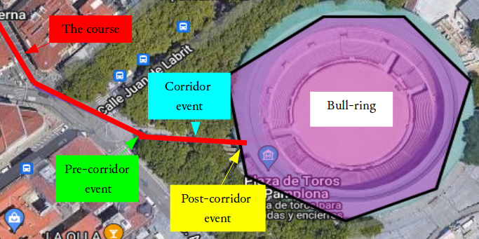
Pre-corridor scenario
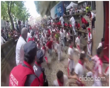
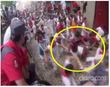
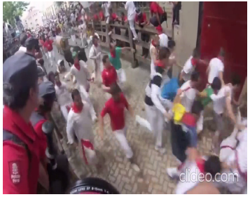
a (t=0 s)	b (t=1.5 s)	c (t=2.5 s)
Corridor scenario
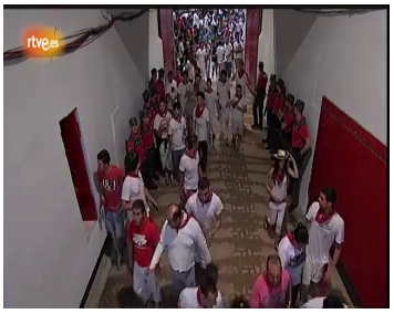
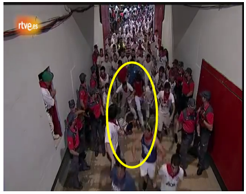
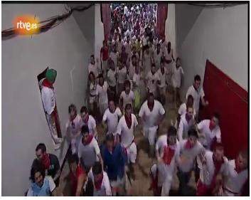
d (t=5 s)	e (t=20 s)	f (t=30 s)
Post-Corridor scenario
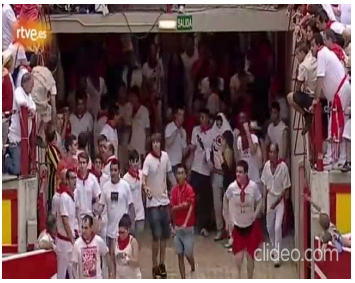
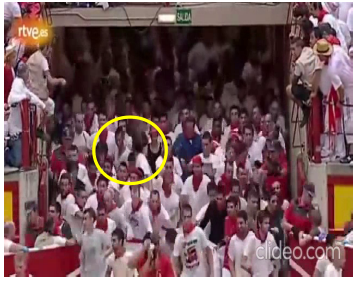
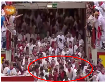
g (t=10 s)	h (t=25 s)	i (t=30 s)

Figure 1: (Color on-line only) (Upper) Layout of the street and locations where the incidents took place. Pre-corridor event (first row), corridor event (second row) and post-corridor event (third row). The snapshots address the time line of the event. The corresponding time-stamp is indicated below the snapshots. The yellow and red circles indicate the region where the first pedestrian stumbles and where the stumbling pedestrians block the exit, respectively. In the last picture (lower right) many pedestrians pile-up (out of the scene).

The following are the feature actions taking place in the events:

• Pre-corridor: One pedestrian stumbles and falls during the rush. Few seconds after, he (she) manages to get up and continues his (her) way out. Neighboring pedestrians run without major incidents.

• Corridor: Three pedestrians stumble and fall during the event. Notice that, unlike the pre-corridor event, they stumble in a higher density scenario. Fortunately, they get up quickly and continue their escaping route.

• Post-corridor: A cluster of more than forty pedestrians stumble and fall during the rush. The video shows that the majority of falls are correlated in both space and time. Unlike the other two events, the first fallen pedestrian is unable to stand up quickly, triggering a massive stumble. Consequently, the crowd evolved towards a completely block scenario (see red circle in Fig. 1).

The very first inspection of the events brings out the fact that the local density around the first falling pedestrian is a crucial feature to the forthgoing events. That is, the higher the local density, the greater tendency towards a massive stumble. We will leave the above matter to Section 5.1.1 and for now we will focus on the data acquisition procedure (see Section 3.1). We will further introduce some definitions in Section 3.2.

3.1 Data acquisition

In order to quantify the three incidents exhibited in Fig. 1, we sampled the movies at a rate of 8 frames per second (attaining a time interval between successive images of 0.125 seconds). The criteria for choosing this sampling period was: 1) The period should be large enough to include (at least) one fallen individual and to achieve a reasonable amount of measurements, 2) during this period, the camera must be fixed to perform the right perspective correction.

The total number of acquired images for the pre-corridor event was 32, while the other two events attained 240 images each. This allowed a semi-manual tracking of the pedestrians by means of the ImageJ software [30]. We made sure that any pedestrian trajectory included at least 10 data points.

3.2 Definitions of relevant magnitudes

The following are the most meaningful magnitudes in the context of our investigation.

• The local density at any position $\vec{r}=(x,y)$ and time $t$ was computed as follows

  $$\rho_{i}(\vec{r},t)=\frac{N_{i}(\vec{r},t)}{\pi R^{2}}$$ (6)

  where $N_{i}(\vec{r},t)$ represents the number of neighbors of pedestrian $i$ within a fix radius $R=1\,$m (see Fig. 2).

• The instantaneous speed (modulus) for each runner was computed as the symmetric incremental ratio

  $$v_{i}(t)=\frac{|\vec{r_{i}}(t+\Delta t)-\vec{r_{i}}(t-\Delta t)|}{2\Delta t}$$ (7)

  for $\Delta t=0.125\,$s,

• The local density gradient around a pedestrian $i$ (modulus) was defined as follows

  $$\nabla\rho_{i}(t)=|N_{f}(t)-N_{b}(t)|$$ (8)

  where $N_{f}$ and $N_{b}$ represent the number of moving pedestrians located in the forward and backward directions, respectively (see Fig. 2 for details). We only considered moving pedestrians for the gradient computation. That is, fallen individuals were excluded from the computation. The $N_{f}$ and $N_{b}$ counts only considered pedestrians within the distance $R=1\,$m to pedestrian $i$ (see Fig. 2).

• We defined the product

  $$f_{s,i}=v_{i}\nabla\rho_{i}$$ (9)

  as a “susceptibility” to the fall. This “susceptibility” accounts for the compound nature of the falling: the pedestrian’s own speed ($v_{i}$) and the pushing environment ($\nabla\rho_{i}$).
  

The sampling area was located in the middle of the pathway, as depicted in Fig. 4a. As already mentioned, each magnitude was recorded every $0.125\,$s.

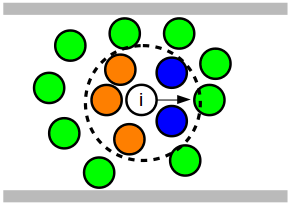
(a)

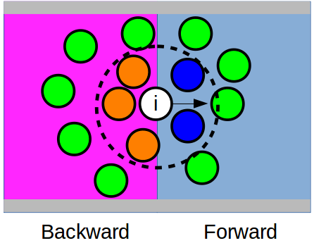
(b)

Figure 2: (Color on-line only) Schematic diagram for the individuals in the corridor. The circles represent pedestrians moving from left to right. The upper and lower lines represent the walls of the corridor. The dashed circle corresponds to the measurement area around pedestrian $i$. In this case, he (she) is surrounded by five individuals ($N_{i}=5$). Therefore, the local density is $\rho=5/\pi$ (p/m${}^{2})$ (see Eq. 6). Also, notice that three of these neighbors are located backward with respect to pedestrian $i$ (orange circles), while the other two are placed forward (blue circles). Therefore, the local gradient density around pedestrian $i$ is $\nabla\rho_{i}=1$ (see Eq. 8).

4 Numerical simulations

4.1 Boundary and initial conditions

In order to study this process, we recreated the “Running of the bulls” event (see Section 3) by placing from 100 up to 700 pedestrians inside a straight corridor of width $w=5\,$m (similar to the width at the entrance of the bull-ring) and length $L=50\,$m. The global density ranged from $\rho=0.5$ to 3 p/m². This is similar to the local density values measured in the analyzed scenes of the San Fermín festival (see Fig. 4).

The individuals were initially distributed at random positions along the simulation box, with random initial velocities according to a Gaussian distribution with null mean value. If certain conditions were met (see Section 4.2), any moving pedestrian could switch his (her) behavior to the “fallen” pedestrian behavior. Fallen pedestrians were those that remained at a fix position until the end of the simulation process.

The desired velocity $v_{d}$ was the same for all the individuals, meaning that all of them had the same anxiety level. The desired direction $\mathbf{\hat{e}_{d}}$ was updated at each time step in order to point to the exit (say, the entrance of the bull-ring) as depicted in Fig. 3.

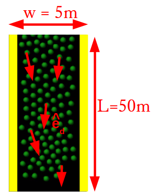
Figure 3: (Color on-line only) Snapshot of simulated evacuation process through a $5\,$m $\times\,50\,$m straight corridor. $\mathbf{\hat{e}_{d}}$ points directly to the exit (say, the entrance of the bull-ring at the bottom of this scheme). All the individuals correspond to “moving pedestrians”. The left and right yellow lines represent the walls of the corridor.

4.2 Moving and fallen pedestrians

We assumed two behavioral patterns, as already mentioned: “moving” individuals and “fallen” individuals. The former are those that move according to Eq. (1). The latter are those that are not able to move at all until the end of the evacuation process. Moving pedestrians, however, are able to switch to the fallen behavior, but fallen pedestrians always remain in the same condition.

The falling transition was implemented as follows. First, we computed the “fallen susceptibility” (say, $f_{s}^{(i)}=v^{(i)}\nabla\rho^{(i)}$) for each moving pedestrian, at instance $i$ (see Eq. 9). Secondly, we switched the state of each “moving” individual to the “fallen” category with the following probabilities

$$p(f_{s}^{(i)})=\left\{\begin{matrix}p_{F}(f_{s}^{(i)})&\mathrm{if~{}there~{}is~{}a~{}fallen~{}individual~{}nearby}\\ p_{NF}(f_{s}^{(i)})&\mathrm{if~{}there~{}is~{}not~{}a~{}fallen~{}individual~{}nearby}\end{matrix}\right.$$ (10)

where fallen neighbors are considered to be within a radius of 1 m. That is, we considered those fallen neighbors located backward and forward the pedestrian $i$. Notice that $p_{F}$ and $p_{NF}$ depend on the susceptibility $f_{s}^{(i)}$, and are obtained from the fitting of experimental data (see Section. 5.1.2 for details on the computation of these probabilities). The time-step between instances was 0.5 s.

The moving pedestrians were allowed to pass through the fallen ones. In order to make this possible, we assumed that no social repulsion was present between the moving and fallen individuals. See Ref. [22] for details.

4.3 Simulation software

The simulations were implemented on the Lammps molecular dynamics simulator [31]. Lammps was set to run on multiple processors. The chosen time integration scheme was the velocity Verlet algorithm with a time step of $10^{-4}\,$s. Any other parameter was the same as in previous works (see Refs. [21, 32]).

We performed between 30 and 100 simulations for each scenario in order to get enough data for statistical analyses (see figures caption for details). Data was sampled at time intervals of 0.05 s along 100 s. The recorded magnitudes were the pedestrian’s positions and velocities for each evacuation process.

5 Results

We present in this section the main results of our investigation. The section is divided into two parts. In the first part (Section 5.1), we present the empirical results extracted from each incident. In the second part (Section 5.2), we compare the empirical results with numerical simulations.

5.1 Empirical results

The analysis of the videos is divided into two separate Sections. The first one examines the crowd behavior previous to the first fallen pedestrian (within the sight of the film), while the second one focuses on the dynamics following the fall. These are two naturally different stages, since the former corresponds to an homogeneous crowds, while the latter deals with two behavioral patterns (i.e. with “moving” and “fallen” pedestrians).

5.1.1 Before the first fall

The analysis started by slicing the scenes shown in Fig. 1. We made the corresponding perspective corrections and computed the magnitudes defined previously in Section 3.2. Fig. 4a schemes the procedure for the computation of each observable.

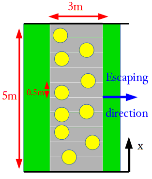
(a) Measuring diagram

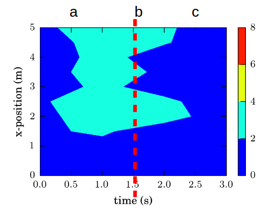
(b) Pre-corridor

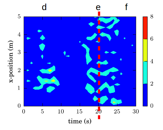
(c) Corridor

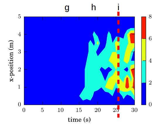
(d) Post-Corridor

Figure 4: (Color on-line only) (a) Schematic diagram for individuals during the running. In order to minimize boundary effects, the measurements were taken from the middle of each scenario (gray box). This box was binned in cells of size $3\,\mathrm{m}\times 0.5\,\mathrm{m}$. (b-c-d) Density contour lines along time for each scenario. The maps were splined to get smoother curves. Each cell of size $0.5\,\mathrm{s}\times 0.5\,\mathrm{m}$ corresponds to the occupancy density at time $t$ in position $x$ (see the measuring diagram). The scale bar on the right is expressed in pedestrians/m². The vertical red dashed line represents the time of the first fall. The letters above each plot mean the corresponding snapshots in Fig. 1. The horizontal and vertical axis represent the time and the pedestrian’s $x-$location in each corridors, respectively. The walls are located at $x=0$ and $x=5$ (bottom and top of each figure).

Figs. 4b-4d show the local density ($\rho$) pattern along time for each scenario (see caption for details). We can notice a common behavior from the contour maps in Fig. 4: the first fall occurs after an increase in the local density. Or, in other words, an increase in the density somehow anticipates a forthcoming fall. This does not mean that any increment in the density naturally yields a falling incident, but sets an environmental condition for expecting it (in the context of the San Fermín festival).

A closer inspection of the scenes before the falls shows that the natural tendency of the pedestrians is to preserve some distance between them while running, presumably because of trying to dodge other runners. However, the upcoming bulls disturb this tendency towards a more chaotic scenario. Consequently, there is no time left for trying to dodge others, and the density increases.

In order to quantify the above observation, we measured the pedestrians’ velocity ($v_{i}$) and the local density gradient ($\nabla\rho$), as defined in Section 3.2. Both magnitudes and some comments on its time evolution can be found in A. However, we actually prefer to focus on the susceptibility $f_{s}$ as defined in Section 3.2. This is, from our point of view, a more meaningful magnitude to express the disturbed scenario.

Fig. 5 shows the susceptibility histograms as a function of time for each scenario (see caption for details). Likewise the local density patterns, we can notice a common behavior from the histograms: the first fall occurs after an increase of the number of pedestrians exposed to high susceptibility values (see white circles in Fig. 5).

Notice that the white circles in Fig. 5 do not enclose a large amount of events (i.e. many counts) but those that are significant to the falling process. This means that only a few pedestrians attain the susceptibility level to (probably) produce a falling incident.

The susceptibility appears as a better indicator for an imminent fall with respect to the local density. Fig. 5 provides a rough threshold (say, $f_{s}\approx 4$) pointing to an imminent fall. The increase in the local density stands for a likely falling condition, although we can not set any clear threshold for the San Fermín context.

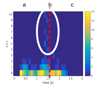
(a) Pre-corridor

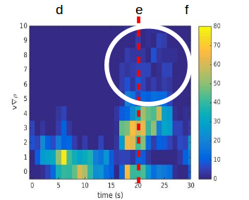
(b) Corridor

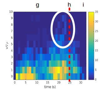
(c) Post-Corridor

Figure 5: (Color on-line only) 2-D histograms for the falling susceptibility ($v\nabla\rho$) along time for each scenario. The scale bar on the right corresponds to the number of pedestrians exposed to $v\nabla\rho$ ($y$-axis) at time $t$ ($x$-axis). The bin size was $0.125\,\mathrm{s}\times 1\,\mathrm{people~{}m/s}$. The vertical red dashed line represents the time-stamp of the first fall. The horizontal and vertical axis represent the time and the falling susceptibility, respectively. For clarity reasons, the upper limit of each color bar is different. The letters above each plot mean the corresponding snapshots in Fig. 1.

5.1.2 After the first fall

We will now focus on the “fallen” pedestrians. We first computed the number of stumbles in presence (or not) of fallen neighbors as a function of time. This is shown in Fig. 6 for the post-corridor scenario only. The pre-corridor and corridor scenes are not shown because the scarcity of data did not allow a reliable analysis.

As can be seen in Fig. 6, near 40 pedestrians stumble and fall in the vicinity of, at least, one fallen neighbor at the end of the process. But this number barely reaches 10 individuals in the absence of a neighboring fallen pedestrian. Thus, it becomes clear that the presence of at least one fallen neighbor increases dramatically the ratio of casualties along time.

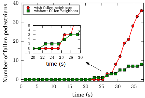
Figure 6: (Color on-line only) Empirical number of fallen pedestrians with (red circles) and without (green squares) fallen neighbors as a function of time in the post-corridor scene.

We further examined the number of fallen neighbors around any new falling pedestrian. The sample probabilities are exhibited in Fig. 7. We estimate a sampling error of $\sigma\approx 0.2$ for each bin (see caption for details). This means that the case of only one fallen neighbor is actually the significant one. More than one fallen neighbors may occur, but its relevancy is still in question according to our data.

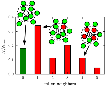
Figure 7: (Color on-line only) Normalized cumulative number of fallen pedestrians as a function of the number of fallen neighbors in the post-corridor scenario. The count of fallen neighbors was done within a fix radius $R=1\,$m. The diagrams above the bins are schematic representations for each case. The dashed circle corresponds to the measurement area around pedestrian $i$. The plot is normalized with respect to the total number of fallen pedestrians. The mean number of fallen individuals in this sample distribution is $\mu=1.83$. The bin error is expected to be $\sigma=\sqrt{p\,(1-p)/6}$ for $p\approx\mu/6$.

The fact that fallen neighbors increase dramatically the possibility of new fallings turned our investigation to the following working hypothesis: the presence of “fallen neighbors” increases the chance of falling, in addition to the expectation for susceptible (moving) individuals alone. This means that those environment attaining “fallen individuals” should be studied separately from the “non-fallen” ones.

We first computed separately the falling probabilities for individuals that belong to an environment with, at least, one fallen neighbor, and with no fallen neighbors at all. We studied both situations as a function of the susceptibility $f_{s}$. The following is the expression used for computing both falling probabilities ($p_{F}$ and $p_{NF}$, see Eq. 10):

$$p(f_{s})=\frac{\displaystyle\sum_{t=0}^{T}N_{F}(f_{s})}{\displaystyle\sum_{t=0}^{T}N_{T}(f_{s})}\\$$ (11)

where $N_{F}$ and $N_{T}$ represent the number of falling pedestrians and the total number of pedestrians (either fallen and moving ones) attaining a falling susceptibility $f_{s}$, respectively. Both sums run over all the discrete time samples (see Section 3.1 for details). Notice that the value of $f_{s}=v\nabla\rho$ was always sampled just before the fall occurs.

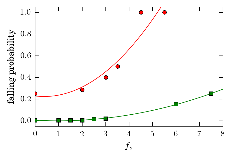
Figure 8: (Color on-line only) Falling probability as a function of the pedestrian’s susceptibility ($f_{s}=v\nabla\rho$) with (red circles) and without (green squares) neighboring fallen pedestrians (see Eq. 11). Solid lines correspond to the quadratic fitting of each data set: $p_{F}(s)=0.33\,f_{s}^{2}-0.025\,f_{s}+0.229$ (red curve) and $p_{NF}(s)=0.006\,f_{s}^{2}-0.011\,f_{s}+0.001$ (green curve).

Fig. 8 shows the falling probability as a function of the susceptibility ($f_{s}$) in the post-corridor scene (see caption for details). It can be seen that the falling probability fits accurately a quadratic function with respect to $f_{s}$ in both environmental conditions (say, with and without fallen neighbors). Moreover, Fig. 8 is in agreement with the rough threshold ($f_{s}\approx 4$) observed in Fig. 5 for an imminent falling. We can now confirm that the probability of falling increases rapidly beyond this value.

Interestingly, both curves exhibit a similar qualitative shape regardless of the environmental condition. The presence of fallen neighbors, however, introduces, at least, an additional $20\%$ of chances for the new fall to occur. This additional probability due to a fallen neighbor increases as $f_{s}$ becomes larger, as can be noticed from the comparison of the slopes in Fig. 8.

Concluding remarks from the empirical results

Our major conclusions from this Section are as follows. First, two different causes of stumbles can be noticed during the rush: a few individuals fall as a consequence of their interaction between other moving pedestrians only. However, the majority stumble in presence of, at least, another fallen pedestrian.

As a second conclusion, we noticed that the falling probability increases as the susceptibility $f_{s}=v\nabla\rho$ (say, the product between the local density gradient and the velocity of each pedestrian) increases. Thus, fallings are more likely to occur whenever people rush away from danger (i.e the bulls) or embody a striking situation (i.e high density gradient). These are the commonly observed situations in the San Fermín festival.

5.2 Numerical results

In this Section we widen the empirical picture of the San Fermín festival by means of numerical simulations. Our first aim is to mimic this situation within the context of the SFM (see Section 2 for details). We introduce falling probabilities to the basic SFM, according to estimates from Section 5.1. We then investigate possible scenarios according to the SFM.

5.2.1 The morphology in the bulk of the crowd

Fig. 9 exhibits a few snapshots of the corridor simulations for different crowd densities. The moving direction is from from top to bottom. The corridor width is similar to the one in San Fermín (see caption for details). The overlapping individuals are actually the ones passing through fallen pedestrians.

$v_{d}=3\,$m/s
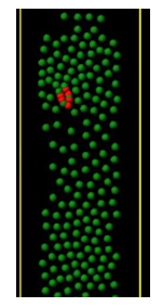
$\rho~{}=~{}1\,$p/m2	$\rho~{}=~{}2\,$p/m2

$v_{d}=5\,$m/s
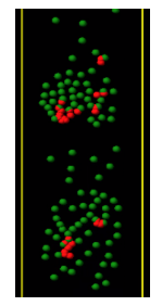
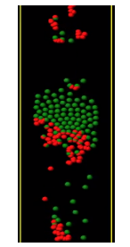
$\rho~{}=~{}1\,$p/m2	$\rho~{}=~{}2\,$p/m2

Figure 9: (Color on-line only) Snapshots of different evacuation processes for two desired velocities and two densities at the time-stamp of 15 s. Moving and fallen pedestrians are represented in green and red circles, respectively. The moving direction is from top to bottom. The yellow lines represent the walls of the pathway. The corridor width is $5\,$m.

The first two columns in Fig. 9 correspond to the lowest value of the explored anxiety levels ($v_{d}=3\,$m/s). We can see that no fallings occur for $\rho=~{}1~{}\,$p/m², but a unique cluster of fallen pedestrians appears for $\rho~{}=~{}2\,$p/m². An inspection of the animations shows that the first fallen runner triggers the falling of neighboring runners. This is in agreement with the falling events reported in the videos, and confirms once more, the relevancy of the first falling.

Interesting, there is an increase in the number of isolated (i.e not in contact) human clusters of fallen pedestrians for the more stressing scenario (last two columns of Fig. 9). This is also in agreement with the empirical patterns exhibited in Fig. 1. Furthermore, the complete video recordings show that stressed pedestrians tend to rush chaotically, and thus, the probability of fallings increases (see Fig. 8).

The fallings shown in Fig. 9 appear somehow related to the overall density of the crowd and the degree of clusterization during the run. Both issues will be studied separately in the next sections.

5.2.2 Number of fallen pedestrians versus the density

Fig 10 shows the number of stumbles occurring during the first 35 s of the escaping process as a function of the global density (see caption for details). We analyzed two desired velocities ($v_{d}=3\,$m/s and $v_{d}=5\,$m/s) since these appear as quite reasonable values according to data in A.

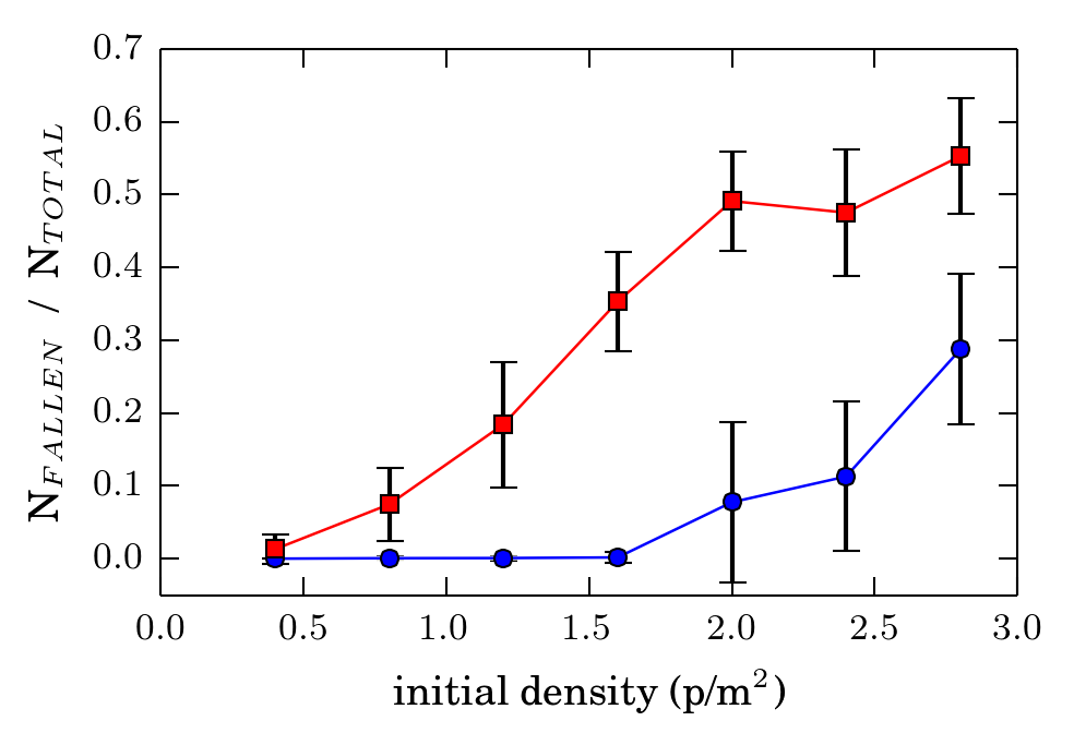
Figure 10: (Color on-line only) Normalized number of fallen pedestrians as a function of the initial density for $v_{d}=3\,$m/s (blue circles) and $v_{d}=5\,$m/s (red squares) during the first 35 s (same corridor as in Fig. 9). Initially, pedestrians were randomly distributed along the simulated corridor. Mean values were computed along 50 realizations. The plot is normalized with respect to the total number of simulated pedestrians. The error bars corresponds to $\pm\sigma$ (one standard deviation).

We can see in Fig. 10 that the number of fallen pedestrians increases monotonically with density. This is an expected result since the more crowded environment, the more strikes between runners, and consequently, the more chances to fall down. These chances also increase with the desired velocity, that is, with the anxiety level of the individuals. Notice that these results are in agreement with in situ videos (see Section 3). Specifically, the snapshots in Fig. 1 show that the stumbles commonly occur in the high density scenario (i.e. in the post-corridor scenario).

We should call the attention on the fact that Fig. 10 computes the fallings regardless of the clusterization context. This opens the question on whether the clusters formation tend to increase the number of fallings or not. We turn to this point in the following Section.

5.2.3 Clusters

We now turn to study the clustering structures, as defined in Section 2.2. We classified the human clusters (of fallen pedestrians) into three categories (according to their size $n$) as follows: small ($1\leq n\leq 5$), medium ($5<n<25$) and big ($n\geq 25$). Fig. 11 shows the mean multiplicity of human clusters for each category (see caption for details).

A very first inspection of Fig. 11 shows that small human clusters have a major role along the whole process (for $v_{d}=5$), while its role at the early stage of the processes appears as essential.

A closer inspection of Fig. 11 shows the following:

• Small human clusters ($1\leq n\leq 5$): The occurrence of small human clusters is greater in the higher stress scenario ($v_{d}=5\,$m/s) than in the lower one ($v_{d}=3\,$m/s), as depicted previously in Fig. 9. This means that, the higher the anxiety level, the most likely that (non contacting) pedestrians can initiate a falling process. This is a very dangerous environmental condition since any pedestrian becomes a potential instance of falling (for himself/herself and others).
  

• Medium human clusters ($5<n<25$): The higher the anxiety level, the more likely to occur. This is somehow engaged to the existence of small clusters since the latter may increase its size (due to new fallings) as the process evolves. In other words, an examination of the process animations shows that small clusters can merge into a medium cluster.
  

• Big human clusters ($n\geq 25$): A single big cluster can be observed in the low stress scenario, while six of them occur in the high stress one. As in the medium human clusters, an inspection of the animations shows that many medium clusters can merge into bigger one.
  

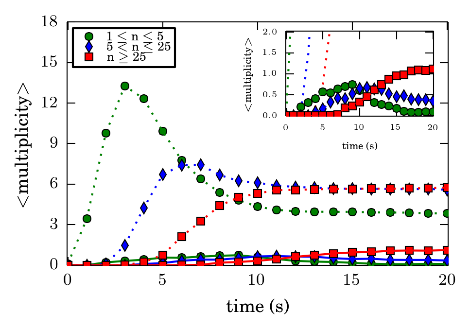
Figure 11: (Color on-line only) Mean multiplicity of human clusters of fallen pedestrians ($n$) for three different size categories (see legend for details) as a function of time. The size of each human cluster was obtained every $1\,$s. Data was acquired from 100 simulation processes. Solid and dashed curves correspond to $v_{d}=3\,$m/s and $v_{d}=5\,$m/s, respectively. The density was $\rho~{}=~{}2\,$p/m².

We resume the highly stressing scenario as the one where fallings occur in many places and fallen clusters of any size are likely to occur. The low stressing scenario is substantially different since people fall around a single cluster.

As a concluding remark, the massive stumble in the post-corridor event shown in Fig. 1 is similar to the above low stressing scenario, attaining a big fallen cluster. We presume that the runners at this instance were quite tired, resembling a low anxiety behavior (in the context of the SFM).

5.2.4 Size of the largest avalanche

Besides the size of the human clusters, we further examined the size of the largest avalanche of fallen pedestrians. That is, the maximum number of new fallen pedestrians (regardless of the falling location). This is, from our point of view, a meaningful magnitude to express the cluster formation rate. Fig. 12 shows the histograms of the largest avalanche distribution for two density levels (see caption for details). We omitted the case $\rho~{}=~{}1\,$p/m² because it does not provide enough falling samples for a proper statistic. We considered in Fig. 12 the densities $\rho~{}=~{}2\,$p/m² and $\rho~{}=~{}3\,$p/m².

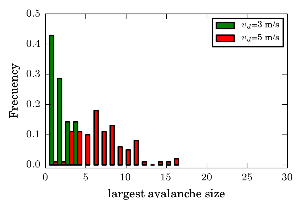
(a) $\rho~{}=~{}2\,$p/m²

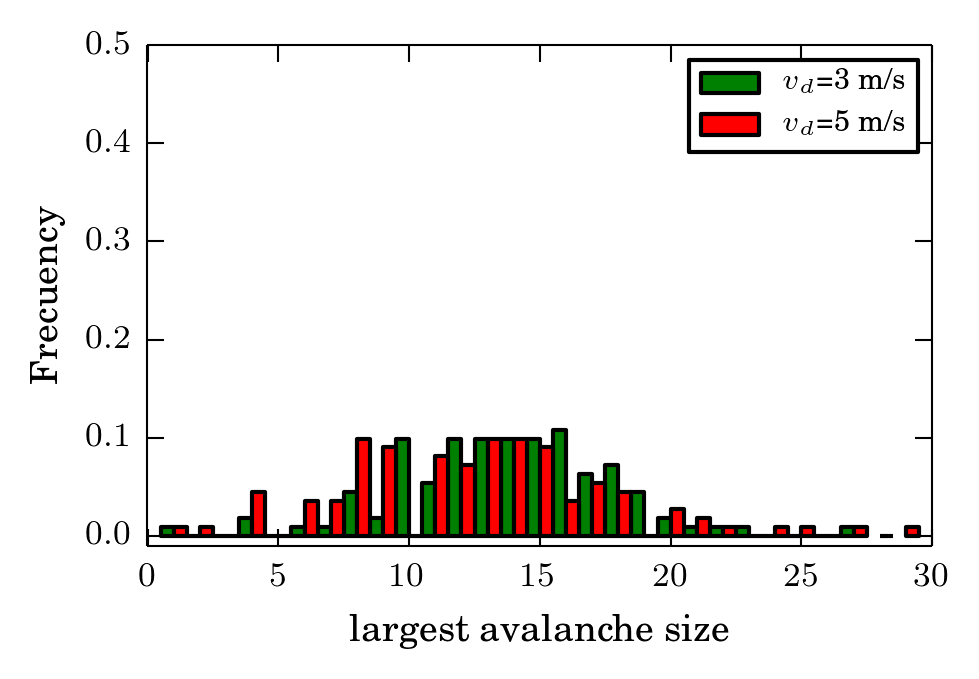
(b) $\rho~{}=~{}3\,$p/m²

Figure 12: (Color on-line only) Normalized distribution of the largest avalanche size for two stress levels and two densities (see legend for details). The bin size is 5 pedestrians. The plot is normalized with respect to the total number of events. Data was recorded from 100 escaping processes.

We first notice that the mean value of the distribution depends on the pedestrian’s anxiety level in the low-density situation ($\rho~{}=~{}2\,$p/m²). As can be seen in Fig. 12a, the (maximum) avalanche events do not involve more than 5 pedestrians for $v_{d}=3\,$m/s, yielding a narrow distribution. But, in the highly anxious situation of $v_{d}=5\,$m/s, the corresponding distribution widens to allow up to 15 or 17 new fallings. This phenomenon appears reasonable since anxious pedestrians rush up to $v\approx v_{d}$, and thus, they become more susceptible to fallings ($f_{s}\approx v_{d}\,\nabla\rho$).

Besides, Fig. 12b shows that the avalanche events, mainly, involve 10 to 15 pedestrians for $\rho=3\,$p/m², regardless of the anxiety level. These are massive events that occur in a quite crowded environment, somewhat similar to the one shown in Fig. 1 for the post-corridor scene. As already observed in Section 5.1, these fallings occur because pedestrians embody striking situations (i.e. high density gradients), regardless of the rushing level. Recall that high density gradients yield highly susceptible conditions for the falling.

We stress the fact that varying the anxiety level does not significantly change the behavior of the largest avalanche distribution. Or, in other words, the avalanches are mainly controlled by density regardless the anxiety level in high-density situation.

Concluding remarks from the numerical results

The results from the numerical simulations show that highly dense environments tend to increase the number of fallings. The final number of fallings, however, is a complex interplay between the crowd density and the pedestrians anxiety level:

• For a moderate environmental density and low anxiety levels ($\rho~{}=~{}2\,$p/m² and $v_{d}=3\,$m/s, respectively), the fallings are expected to occur in small avalanches at a single location. Thus, the picture is of a single cluster of fallen pedestrians.

• For a moderate environmental density but high anxiety levels ($\rho~{}=~{}2\,$p/m² and $v_{d}=5\,$m/s, respectively), the fallings occur at many locations and can involve a varying number of falling people each.

• For more crowded environments (say, $\rho~{}=~{}3\,$p/m²), the anxiety level looses significance since the pedestrians strike among others, no matter their escaping desire.

6 Conclusions

Our research focused on the microscopic analysis of the stumbling phenomena during an emergency situation (the Running of th Bulls’ Festival at San Fermín). We first analyzed three real life videos of the rush and proposed a stumbling mechanism in the context of the SFM. We then performed ex post simulations for evaluating the accuracy of the model improvements.

In order to properly understand the stumbling mechanism, we examined the crowd behavior before and after the first falling event. This allowed us to distinguish between an homogeneous scenario (with “moving” pedestrians) and an heterogeneous one (with “moving” and “fallen” pedestrians).

We identified the product between the local density gradient and the velocity of each pedestrian (named here as susceptibility $f_{s}$) as a good indicator for an imminent fall. We noticed that $f_{s}$ is monotonically related to the falling probability. This relation can be found in Section 5.1.

We further noticed through the experimental data that the presence of fallen pedestrians dramatically increases the falling probability of neighboring pedestrians. Our computations show that the latter have, at least, an additional $20\%$ of chances for falling down. Thus, the presence or not of a fallen neighbor is a crucial feature of pedestrians (local) environment. This is actually the main achievement of our investigation.

The pedestrian’s own susceptibility and the presence (or not) of fallen neighbors are the only features allowing a stumble within the context of the Social Force Model. Although the simplicity of this model, we attained fairly good agreement with empirical data from the San Fermín Festival.

We performed ex-post simulations of the “Running of the Bulls”. We used different sets of densities ($\rho$) and anxiety levels ($v_{d}$) for mimicking three instances of the race (see Section 5.2). Our results reproduced satisfactorily the corresponding video recordings for adequate values of $\rho$ and $v_{d}$. We further focused on $v_{d}=3\,$m/s and $v_{d}=5\,$m/s for a detailed analysis of the stumbling process (see Section 5.2). The conclusions are as follows:

• The moderately dense scenarios ($\rho~{}=~{}2\,$p/m²) may evolve quite differently, according to the anxiety level. If $v_{d}=3\,$m/s (low anxiety level) a small stumbling process can takes place at a single location. In this case, we will observe single cluster of fallen pedestrians. However, if $v_{d}=5\,$m/s (high anxiety level) the stumbling process may take place in multiple places within the crowd. Indeed, we observe a varying number of people at falling and clusters of fallen pedestrians among the crowd.

• The highly dense scenario ($\rho~{}=~{}3\,$p/m²) may evolve in the same way, no matter the anxiety level (within our explored range). This way will show up as a massive avalanche within the crowd.

Appendix A Velocity and local density gradient histograms

Fig. 13 shows the velocity histograms as a function of time for each scenario (see caption for details). We observe that, likewise the local density pattern (see Figs. 4b-4d), the three scenarios present a common behavior: the first fall occurs after an increase in the number of pedestrians attaining high velocity (say, $v>2\,$m/s).

A careful inspection of the scenes before the falls shows that some pedestrians moving with high velocity trigger the run of many other relaxed individuals. Consequently, this “fear spreading” among the crowd makes the maximum of the velocity distribution to move towards higher values.

The local density gradient histograms along time for each scenario can be found in Fig. 13 (see caption for details). Notice that this magnitude carries information on the local density profile around each pedestrian (see Eq. 8). That is, the higher the local density gradient, the greater the local density asymmetry in the front–back direction. And therefore, the higher the force unbalance on the corresponding pedestrian.

It can be noticed that there is an increment in the occurrence of high local density gradients (say, $\nabla\rho>1$) few seconds before the first falling. In this sense, in the pre-corridor and post-corridor scenarios, a sizable portion of the pedestrians experienced a significant amount of unbalance in the front-back forces (say, $\nabla\rho\geq 3$). Notice that this is not significant in the corridor scenario.

Velocity
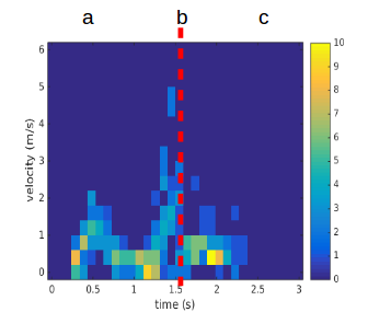
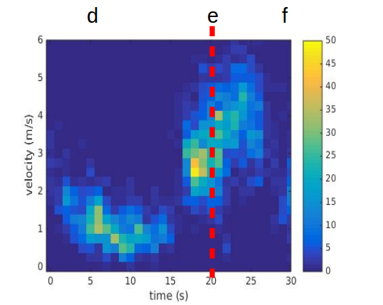
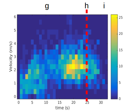
Pre-corridor	Corridor	Post Corridor
Local density gradient
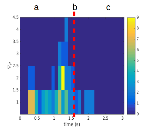
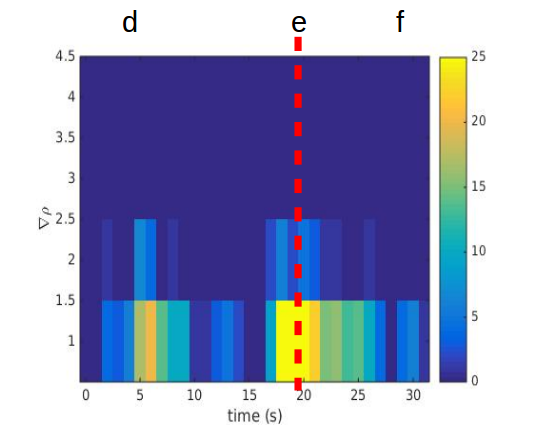
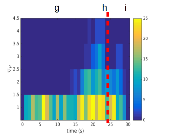
Pre-corridor	Corridor	Post Corridor

Figure 13: (Color on-line only) 2-D histograms for the velocity (upper) and local density gradient (lower) for each scenario. The horizontal and vertical axis represent the time and the measured value of each magnitude, respectively. The bin size was $0.125\,\mathrm{s}\times 0.33\,\mathrm{m/s}$ and $0.125\,\mathrm{s}\times 1\,\mathrm{people}$ for the velocity and the local density gradient, respectively. The vertical red dashed line represents the time of the first fall. Also, for clarity reasons, the upper limit of each color bar is different. The crowd states at different moments (see letters above figures) can be seen in Fig. 1.

References

References

- [1] M. Haghani, M. Sarvi, Z. Shahhoseini, When ‘push’ does not come to ‘shove’: Revisiting ‘faster is slower’ in collective egress of human crowds, Transportation Research Part A: Policy and Practice 122 (2019) 51 – 69.
- [2] W. Jianyu, M. Jian, L. Peng, C. Juan, F. Zhijian, L. Tao, M. Sarvi, Experimental study of architectural adjustments on pedestrian flow features at bottlenecks 2019 (8) (2019) 083402.
- [3] J. W. Adrian, M. Boltes, S. Holl, A. Sieben, A. Seyfried, Crowding and queuing in entrance scenarios: Influence of corridor width in front of bottlenecks, 2018.
- [4] A. Garcimartín, D. R. Parisi, J. M. Pastor, C. Martín-Gómez, I. Zuriguel, Flow of pedestrians through narrow doors with different competitiveness, Journal of Statistical Mechanics: Theory and Experiment 2016 (4) (2016) 043402.
- [5] W. Liao, A. Seyfried, J. Zhang, M. Boltes, X. Zheng, Y. Zhao, Experimental study on pedestrian flow through wide bottleneck, Transportation Research Procedia 2 (2014) 26 – 33, the Conference on Pedestrian and Evacuation Dynamics 2014 (PED 2014), 22-24 October 2014, Delft, The Netherlands.
- [6] W. Daamen, S. Hoogendoorn, Emergency door capacity: Influence of door width, population composition and stress level, Fire Technology 48 (2012) 55–71.
- [7] J. Liddle, A. Seyfried, B. Steffen, W. Klingsch, T. Rupprecht, A. Winkens, M. Boltes, Microscopic insights into pedestrian motion through a bottleneck, resolving spatial and temporal variations.
- [8] A. Seyfried, O. Passon, B. Steffen, M. Boltes, T. Rupprecht, W. Klingsch, New insights into pedestrian flow through bottlenecks, Transport. Sci. 43 (2007) 395–406.
- [9] J. Liddle, A. Seyfried, W. Klingsch, T. Rupprecht, A. Schadschneider, A. Winkens, An experimental study of pedestrian congestions: Influence of bottleneck width and length.
- [10] D. Parisi, C. Dorso, Microscopic dynamics of pedestrian evacuation, Physica A 354 (2005) 606–618.
- [11] D. Parisi, C. Dorso, Morphological and dynamical aspects of the room evacuation process, Physica A 385 (2007) 343–355.
- [12] I. M. Sticco, F. E. Cornes, G. A. Frank, C. O. Dorso, Beyond the faster-is-slower effect, Phys. Rev. E 96 (2017) 052303.
- [13] F. Cornes, G. Frank, C. Dorso, Microscopic dynamics of the evacuation phenomena in the context of the social force model, Physica A: Statistical Mechanics and its Applications 568 (2021) 125744.
- [14] D. Helbing, I. Farkas, T. Vicsek, Simulating dynamical features of escape panic, Nature 407 (2000) 487–490.
- [15] R. Hidalgo, C. Lozano, I. Zuriguel, A. Garcimartín, Force analysis of clogging arches in a silo, Granular Matter 15.
- [16] E. T. Owens, K. E. Daniels, Sound propagation and force chains in granular materials, 2011.
- [17] S. Ardanza-Trevijano, I. Zuriguel, R. Arévalo, D. Maza, A topological method to characterize tapped granular media from the position of the particles.
- [18] C. Giusti, L. Papadopoulos, E. Owens, K. Daniels, D. Bassett, Topological and geometric measurements of force chain structure, Physical Review E 94.
- [19] L. Papadopoulos, J. G. Puckett, K. E. Daniels, D. S. Bassett, Evolution of network architecture in a granular material under compression, Phys. Rev. E 94 (2016) 032908.
- [20] L. Papadopoulos, M. A. Porter, K. E. Daniels, D. S. Bassett, Network analysis of particles and grains, Journal of Complex Networks 6 (4) (2018) 485–565.
- [21] G. Frank, C. Dorso, Room evacuation in the presence of an obstacle, Physica A 390 (2011) 2135–2145.
- [22] F. Cornes, G. Frank, C. Dorso, High pressures in room evacuation processes and a first approach to the dynamics around unconscious pedestrians, Physica A: Statistical Mechanics and its Applications 484 (2017) 282 – 298.
-
[23]
[link].
URL https://www.youtube.com/watch?v=qwtu9p2CzGc&ab_channel=DiariodeNavarra -
[24]
[link].
URL https://www.youtube.com/watch?v=5HBvOu08JDI&ab_channel=ELPARDALInformativoCofrade -
[25]
[link].
URL https://www.youtube.com/watch?v=5L4V79NN9aU&ab_channel=Jos%C3%A9LuisVarela - [26] D. Helbing, P. Molnár, Social force model for pedestrian dynamics, Physical Review E 51 (1995) 4282–4286.
- [27] I. Sticco, G. Frank, C. Dorso, Effects of the body force on the pedestrian and the evacuation dynamics, Safety Science 121 (2020) 42 – 53.
- [28] I. Sticco, G. Frank, C. Dorso, Social force model parameter testing and optimization using a high stress real-life situation, Physica A: Statistical Mechanics and its Applications 561 (2021) 125299.
- [29] A. Strachan, C. O. Dorso, Fragment recognition in molecular dynamics, Phys. Rev. C 56 (1997) 995–1001.
- [30] Rasband, W.S., ImageJ, U. S. National Institutes of Health, Bethesda, Maryland, USA, https://imagej.nih.gov/ij/, 1997-2016, Imagej.
- [31] S. Plimpton, Fast parallel algorithms for short-range molecular dynamics, Journal of Computational Physics 117 (1) (1995) 1 – 19.
- [32] G. Frank, C. Dorso, Evacuation under limited visibility, International Journal of Modern Physics C 26 (2015) 1–18.