Enhanced eigenvector sensitivity and algebraic classification of sublattice-symmetric exceptional points

Abstract

Exceptional points (EPs) are degeneracy of non-Hermitian Hamiltonians, at which the eigenvalues, along with their eigenvectors, coalesce. Their orders are given by the Jordan decomposition. Here, we focus on higher-order EPs arising in fermionic systems with a sublattice symmetry, which restricts the eigenvalues of the Hamitlonian to appear in pairs of $\{E,-E\}$. Thus, a naive prediction might lead to only even-order EPs at zero energy. However, we show that odd-order EPs can exist and exhibit enhanced sensitivity in the behaviour of eigenvector-coalescence in their neighbourhood, depending on how we approach the degenerate point. The odd-order EPs can be understood as a mixture of higher- and lower-valued even-order EPs. Such an anomalous behaviour is related to the irregular topology of the EPs as the subspace of the Hamiltonians in question, which is a unique feature of the Jordan blocks. The enhanced eigenvector sensitivity can be described by observing how the quantum distance to the target eigenvector converges to zero. In order to capture the eigenvector-coalescence, we provide an algebraic method to describe the conditions for the existence of these EPs. This complements previous studies based on resultants and discriminants, and unveils heretofore unexplored structures of higher-order exceptional degeneracy.

I Introduction

Exceptional degeneracy is a phenomenon where the eigenvalues of a matrix cross each other and their eigenvectors collapse simultaneously, losing the linear independence [1, 2, 3, 4, 5]. The simplest example is when two eigenvalues and their corresponding eigenvectors coalesce, leading to an exceptional point (EP) of second order. Such singularities can arise in the context of a great variety of physical problems, such as dissipative processes captured by non-Hermitian Hamiltonians [6, 7, 8, 9, 10, 11, 12, 13, 14, 15, 16, 17, 18, 19, 20, 21, 22, 23], and topological phase transitions in chiral Hamiltonians [24, 25]. Their singular behaviour manifests itself in enhanced sensitivity, and thus has potential applications in detection and sensors [26, 27, 28, 29, 30, 31, 32].

An $n^{\rm{th}}$-order exceptional point (EP_n) [33, 34, 35, 36, 37, 38, 39, 40] appears when the Jordan decomposition of the matrix contains an $n$-dimensional (with $n>1$) Jordan block $J_{n}(E)$ along its diagonal, at the eigenvalue $E$. Near an EP₂, the dispersion varies as a square root, viz., $\delta E\sim\sqrt{|\delta\mathbf{q}|}$, where $|\delta\mathbf{q}|$ characterizes the deviation from the EP in the momentum space spanned by the vector $\mathbf{q}$. The derivative of the dispersion diverges at the EP, implying that the change in eigenvalue becomes more and more sensitive as we approach the EP. Such a sensitivity is further enhanced at a higher-order EP_n ($n>2$), because now an $n^{\rm{th}}$-order root sensitivity (i.e., $\delta E\sim|\delta\mathbf{q}|^{1/n}$) can appear in the vicinity of the EP_n for generic situations [37, 38, 40]. The eigenvalue overlap at higher-order EPs can be captured by equations involving discriminants [40] or resultants [38]. However, another important and unique property of an EP, namely the coalescence of eigenstates, remains elusive under this approach. Moreover, the space spanned by the exceptional degeneracy is not a closed subspace of the parameter space of the corresponding matrix [41]. In fact, this space has a finer topological structure beyond the solutions captured by continuous functions (such as the discriminants and resultants) of the matrix.

In this paper, we use an algebraic method to classify the higher-order EPs according to their eigenvector-coalescence. We focus on the nature of the higher-order EPs that can appear in two-dimensional (2d) systems in the presence of a sublattice symmetry [cf. Fig. 1(a)], and determine how their eigenstates collapse. The main results are summarized in Fig. 1(b) and Table 1. Remarkably, according to our classification, all EP_n’s can be categorized into two types. A regular EP_n exhibits a typical $n$-fold eigenvector-coalescence, while a mixed-type EP_n can exhibit different eigenvector-coalescence depending on how our Hamiltonian is approaching it in the parameter space.

The model is implemented by considering $N$ flavours of fermions, living on a bipartite lattice, whose creation operators are given by ${c^{\alpha}_{1}}^{\dagger}$ and ${c^{\alpha}_{2}}^{\dagger}$($\alpha\in[1,N]$). The degrees of freedom for the two sublattices have been distinguished by the subscripts $1$ and $2$. The sublattice symmetry ensures that the Hamiltonian $H$ obeys $P\,H\,P=-H$ [42, 43], with the operator $P$ acting as $c^{\alpha}_{1}\xrightarrow{P}c^{\alpha}_{1}$ and $c^{\alpha}_{2}\xrightarrow{P}-c^{\alpha}_{2}$. This is a very natural condition when the Hamiltonian contains only hoppings from sublattice $1$ to sublattice $2$. Examples of such Hamiltonians include solvable spin liquid models, such as the Kitaev spin liquid [44] (corresponding to $N=1$), and the Yao-Lee $SU(2)$ spin liquid [45] (corresponding to $N=3$). In Hermitian systems, the sublattice symmetry can be viewed as the product of time-reversal transformation and particle-hole transformation of fermions, which translates to a chiral symmetry [42]. In the momentum space, a generic non-Hermitian Hamiltonian with the sublattice symmetry can be brought to the block off-diagonal form:

$$H(\mathbf{q})=\begin{pmatrix}0&i\,\mathbf{B}(\mathbf{q})\\ -i\,\mathbf{B}^{\prime}(\mathbf{q})&0\\ \end{pmatrix},$$ (1)

where $\mathbf{B}$ and $\mathbf{B}^{\prime}$ are $N\times N$ matrices. In order to demonstrate our results in closed analytical forms, we will focus on the $N=2$ case, where the system can be described by $4\times 4$ matrices.

We will characterize our EPs based on the nilpotency of Jordan blocks in the generalized eigenspace. To explain the terminologies, let us consider the example of an EP₃. Near an EP₃, we have a three-dimensional Jordan block, and the Hamiltonian can be expressed as

$$V\,H(\mathbf{q}_{\ast})\,V^{-1} =\textrm{diag}\{J_{3}(E_{1}),\,E_{2},\,E_{3},\,\dots\}$$

$$=\begin{pmatrix}E_{1}&1&0&0&0&\dots\\ 0&E_{1}&1&0&0&\dots\\ 0&0&E_{1}&0&0&\dots\\ 0&0&0&E_{2}&0&\dots\\ 0&0&0&0&E_{3}&\dots\\ \vdots&\vdots&\vdots&0&0&\ddots\\ \end{pmatrix},$$ (2)

where $E_{1}$ is a three-fold degenerate eigenvalue with only one linearly independent eigenvector proportional to $e_{1}=V\,(1,\,0,\,\dots)^{T}$. The generalized eigenspace $\mathcal{L}_{E_{1}}$ of $E_{1}$ includes two other vectors, viz., $e_{2}=V\,(0,\,1,\,0,\,\dots)^{T}$, and $e_{3}=V\,(0,\,0,\,1,\,0,\,\dots)^{T}$, such that $(H-E_{1})$ is nilpotent in $\mathcal{L}_{E_{1}}$. In other words, $(H-E_{1})\,e_{3}=e_{2}$, $(H-E_{1})\,e_{2}=e_{1}$, and $(H-E_{1})\,e_{1}=0$. Intuitively, this EP₃ is interpreted as the singular point where the three eigenvectors of $E_{1}$ collapse into one. According to the Jordan decomposition, we denote the point $\mathbf{q}=\mathbf{q}_{\ast}$ as a simple EP₃, if all the Jordan blocks belonging to the other eigenvalues $E_{2},\,E_{3},\,\dots$ are trivial (i.e., one-dimensional). If the Hamiltonian has more than one eigenvalue whose Jordan block is nontrivial (i.e., has dimension greater than unity), we denote the point $\mathbf{q}=\mathbf{q}_{\ast}$ as a compound EP.

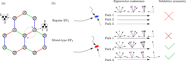
Figure 1: (a) Decorated honeycomb lattice model of fermions with $N=3$ flavours [45], also dubbed as the “Yao-Lee” model (see Appendix E). The system has a sublattice symmetry when only nearest-neighbour hoppings are included in the Hamiltonian. The fermions are labelled by their sublattice indices $A$ and $B$, together with their flavour index $\alpha\in\{1,2,3\}$ on each sublattice site. (b) The coalescence of eigenvectors for a four-band model near a regular EP₃ (blue oval disc) and a mixed-type EP₃ (red oval disc). Near the regular EP₃, three eigenvectors out of the four are collapsing to a single eigenvector at the EP. Near the mixed-type EP₃, how the eigenvectors coalesce strongly depends on the path chosen to approach the EP. There can be two-fold, three-fold, and four-fold eigenvector-coalescence for the three different paths indicated by the dash-dotted, solid, and dashed lines, respectively. When sublattice symmetry is imposed, the three-fold eigenvector-coalescence is forbidden.

The paper is organized as follows. In Sec. II, we discuss the sublattice symmetry and the nature of the EPs, which is the main result of this paper. Sec. III focusses on the properties of various types of EPs and the analytical solutions of eigenvectors in their neighbourhoods. In Sec. IV, we use a quantum distance to characterize the eigenvector folding near an EP, and explain the enhanced eigenvector sensitivity in terms of the unique subspace topology for non-Hermitian matrices. Sec. V deals with some explicit realizations of the systems discussed, and also touches upon the predictions for generic $N$-values. We conclude with a summary and outlook in Sec. VI. Appendices A–E show the details of the mathematical derivations of various results mentioned in the main text.

II Sublattice symmetry and the EP parameter space

The sublattice symmetry makes the characteristic polynomial of the Hamiltonian even in the eigenvalue $E$, as captured by the relation $\det(E-H)=\det[P\,(E-H)\,P]=\det(E+H)$, where we use the fact that the dimension of $H$ is even. The eigenvalues of $H$ thus always come in pairs of $\{E,-E\}$. A natural choice of basis under the sublattice symmetry is to group the upper and lower components of the eigenstates as $\psi$ and $\chi$, respectively. With this choice, the eigenvalue problem is reduced to the following equations:

$$E^{2}\,\psi(\mathbf{q}) =\mathbf{B}(\mathbf{q})\cdot\mathbf{B}^{\prime}(\mathbf{q})\,\psi(\mathbf{q}),\,E\,\chi(\mathbf{q})=-i\,\mathbf{B}^{\prime}(\mathbf{q})\,\psi(\mathbf{q})\,,$$

$$E^{2}\,\chi(\mathbf{q}) =\mathbf{B}^{\prime}(\mathbf{q})\cdot\mathbf{B}(\mathbf{q})\,\chi(\mathbf{q})\,,\,E\,\psi(\mathbf{q})=i\,\mathbf{B}(\mathbf{q})\,\chi(\mathbf{q})\,.$$ (3)

The above indicates that if $(\psi^{T},\,\chi^{T})^{T}$ is an eigenvector for the eigenvalue $E$, $(\psi^{T},\,-\chi^{T})^{T}$ is an eigenvector for $-E$. Besides eigenvalues, the sublattice symmetry also imposes the constraint that nondegenerate eigenvectors should appear in pairs.

The above pairing relation for eigenvectors at $E$ and $-E$ also applies to generalized eigenvectors, which include other linearly independent vectors in the generalized eigenspaces $\mathcal{L}_{E}$ and $\mathcal{L}_{-E}$, apart from the eigenvectors. If we take two generalized eigenvectors $(\psi_{1},\,\chi_{1})$ and $(\psi_{2},\,\chi_{2})$, corresponding to an eigenvalue $E$ having a nontrivial Jordan block, then $(H-E)\,(\psi^{T}_{2},\chi^{T}_{2})^{T}=(\psi^{T}_{1},\,\chi^{T}_{1})^{T}$ is also in the generalized eigenspace of $E$. By applying $P$ to this equation, one can verify that $(H+E)\,(-\psi^{T}_{2},\,\chi^{T}_{2})^{T}=(\psi^{T}_{1},\,-\chi^{T}_{1})^{T}$. Therefore, if $\{(\psi^{T}_{1},\chi^{T}_{1})^{T}$, $(\psi^{T}_{2},\chi^{T}_{2})^{T}$, $(\psi^{T}_{3},\,\chi^{T}_{3})^{T},\,\dots\}$ generate the generalized eigenspace $\mathcal{L}_{E}$, the eigenvectors $\{(\psi^{T}_{1},\,-\chi^{T}_{1})^{T}$, $(-\psi^{T}_{2},\,\chi^{T}_{2})^{T}$, $(\psi^{T}_{3},\,-\chi^{T}_{3})^{T},\,\dots\}$ generate the generalized eigenspace $\mathcal{L}_{-E}$.

According to the above analysis, the degeneracy of the system should be distinguished depending on whether it involves a zero or nonzero eigenvalue $E$ as follows:
(1) If all the eigenvalues are nonzero (i.e., $E\neq 0$), the lower component is linearly related to the upper component as $\chi=-i\,\mathbf{B}^{\prime}(\mathbf{q})\,\psi(\mathbf{q})/E$. The problem is then entirely determined by the $2\times 2$ matrix $\mathbf{B}(\mathbf{q})\cdot\mathbf{B}^{\prime}(\mathbf{q})$. If $E$ is an eigenvalue where two eigenvectors coalesce at the momentum $\mathbf{q}=\mathbf{q}_{\ast}$, then $-E$ shows an identical behaviour. Hence, the exceptional degeneracy for $E\neq 0$ must be a compound EP, always appearing as a doublet of EP₂’s.
(2) If $E=0$ is an eigenvalue with algebraic multiplicity $l$, the corresponding eigenvector is obtained from the kernels of the two matrices, i.e., those $\psi$ and $\chi$ which satisfy $\mathbf{B}(\mathbf{q})\,\chi=0$ and $\mathbf{B}^{\prime}(\mathbf{q})\,\psi=0$. The eigenvectors are given by $(\psi^{T},0)^{T}$ and $(0,\chi^{T})^{T}$. Assuming that the numbers of solutions to the two equations are $\dim(\ker\mathbf{B})=m$ and $\dim(\ker\mathbf{B}^{\prime})=n$, respectively, we can construct $(m+n)$ distinct eigenvectors. Hence, the order of the EP can range from $2$ to $(l+1-m-n)$.

From the two possible cases, we find that the $E=0$ situation gives us the richest EP structure, and hence, this will be the focus of the rest of this paper. Denoting the eigenvalues of $\mathbf{B}(\mathbf{q})\cdot\mathbf{B}^{\prime}(\mathbf{q})$ for $N=2$ as $\lambda$, the dispersion can be generically written as $\lambda\sim|\delta\mathbf{q}|$ or $\lambda\sim|\delta\mathbf{q}|^{1/2}$, in the vicinity of the EP, where $\delta\mathbf{q}=\mathbf{q}-\mathbf{q}_{\ast}$. According to Eq. (3), the dispersion then takes the form $E\sim|\delta\mathbf{q}|^{1/2}$ or $E\sim|\delta\mathbf{q}|^{1/4}$.

Different types of EPs for $N=2$
$SU(2)$ doublet of EP2	EP4	EP3
$\mathbf{B}=0$, $\mathbf{B}^{\prime}\propto\mathbb{I}$	$\dim(\ker\mathbf{B})+\dim(\ker\mathbf{B}^{\prime})=1$,              $\ker(\mathbf{B}\,\mathbf{B}^{\prime})=\mathrm{im}(\mathbf{B}\,\mathbf{B}^{\prime})$	$\dim(\ker\mathbf{B})=\dim(\ker\mathbf{B}^{\prime})=1$, $\textrm{im}\,(\mathbf{B}^{\prime})=\ker(\mathbf{B})$, $\textrm{im}\,(\mathbf{B})\neq\ker(\mathbf{B}^{\prime})$
$H(\mathbf{q}_{\ast})=\mathrm{diag}\{J_{2}(0),J_{2}(0)\}$	$H(\mathbf{q}_{\ast})=J_{4}(0)$	$H(\mathbf{q}_{\ast})=\mathrm{diag}\{J_{3}(0),0\}$
$\mathbf{B}=\begin{pmatrix}0&0\\ 0&0\\ \end{pmatrix}$, $\mathbf{B}^{\prime}=\begin{pmatrix}b^{\prime}&0\\ 0&b^{\prime}\\ \end{pmatrix}$	$\mathbf{B}^{\prime}=\begin{cases}\begin{pmatrix}b^{\prime}_{1}&b^{\prime}_{2}\\ b^{\prime}_{3}&0\\ \end{pmatrix},&\textrm{when }\mathbf{B}=\begin{pmatrix}0&0\\ 0&b_{4}\\ \end{pmatrix}\\ &\\ \begin{pmatrix}b^{\prime}_{1}&b^{\prime}_{2}\\ 0&b^{\prime}_{4}\\ \end{pmatrix},&\textrm{when }\mathbf{B}=\begin{pmatrix}0&b_{2}\\ 0&0\\ \end{pmatrix}\end{cases}$	$\mathbf{B}=\begin{pmatrix}p_{1}\,u_{1}&p_{1}\,u_{2}\\ p_{2}\,u_{1}&p_{2}\,u_{2}\end{pmatrix}$,    $\mathbf{B}^{\prime}=\begin{pmatrix}u_{2}\,p^{\prime}_{2}&-u_{2}\,p^{\prime}_{1}\\ -u_{1}\,p^{\prime}_{2}&u_{1}\,p^{\prime}_{1}\end{pmatrix}$

Table 1: Explanation of the conditions for the existence of different types of EPs when $N=2$. The forms of the matrices $\mathbf{B}$ and $\mathbf{B}^{\prime}$ at the degenerate point $\mathbf{q}=\mathbf{q}_{\ast}$ are shown. Since there is an obvious symmetry under the exchange $\mathbf{B}\leftrightarrow\mathbf{B}^{\prime}$, every case displayed in the table has a $\mathbf{B}\leftrightarrow\mathbf{B}^{\prime}$ partner. The parameters in the bottom row need to further satisfy (1) $b^{\prime}\neq 0$ in the first column; (2) $\det(\mathbf{B}^{\prime})\neq 0$ and $\mathbf{B}\neq 0$ in the second column; (3) $|u_{1}|^{2}+|u_{2}|^{2}\neq 0$, $|p_{1}|^{2}+|p_{2}|^{2}\neq 0$, $|p^{\prime}_{1}|^{2}+|p^{\prime}_{2}|^{2}\neq 0$, and $p^{\prime}_{1}\,p_{2}-p^{\prime}_{2}\,p_{1}\neq 0$ in the third column.

After defining the model, our goal is to work out the Hamiltonian along with the eigenvectors at $E=0$, as well as the nontrivial generalized eigenspace $\mathcal{L}_{0}$. At an $n^{\rm{th}}$-order EP, a series of vectors $\{e_{0},\,e_{1},\,e_{2},\,\dots,\,e_{n}\}$ satisfies the chain equations $H\,e_{j}=e_{j-1}$, with $e_{0}$ denoting the null vector and $e_{1}$ the eigenvector (for $E=0$). When there is no symmetry, the corresponding parameter space of the Hamiltonian, denoted by $\mathcal{EP}_{n}$, can be figured out easily using the standard methods [41] (cf. Appendix C). However, in the presence of sublattice symmetry, employing the standard formalism usually becomes complicated, because it is difficult to find out all the matrices that commute with both the Jordan decomposition and the symmetry transformation. To avoid this issue, we instead employ the decomposition of each eigenstate as $e_{j}=(\psi^{T}_{j},\,\chi^{T}_{j})^{T}$, such that the condition for the existence of a higher-order EP simplifies to $(i\,\mathbf{B}\,\chi_{j},-i\,\mathbf{B}^{\prime}\,\psi_{j})=(\psi_{j-1},\,\chi_{j-1})$. As we have already shown that $e_{1}$ is related to the kernels of $\mathbf{B}$ and $\mathbf{B}^{\prime}$, the chain equations can be solved step by step. The condition for the existence of an EP requires a series of relations between the images $\{\mathrm{im}(\mathbf{B}),\,\mathrm{im}(\mathbf{B}^{\prime})\}$ and the kernels $\{\ker(\mathbf{B}),\,\ker(\mathbf{B}^{\prime})\}$. From these algebraic relations, we can explicitly work out $\mathcal{EP}_{n}$. The results are summarized in Table 1 (with the derivation shown in Appendix A). We can clearly infer that the results in Table 1 cannot be obtained from solutions of some simple continuous equations derived from the Hamiltonian. Hence, a non-Hermitian system exhibits a much richer structure for degeneracies, compared to a Hermitian degeneracy, as observed in the case of no symmetry [41].

III The eigenvector structures of different types of EPs for $SU(2)$

In the following subsections, we discuss the properties of various possible EP_n’s in great detail, especially focussing on the analytic solutions for the eigenvectors. The system with $N\geq 2$ can host both EP₂’s and higher-order EPs, which we discuss below on a case-by-case basis for $N=2$. We denote the location of an EP by $\mathbf{q}=\mathbf{q}_{\ast}$, and use $\delta\mathbf{q}=\mathbf{q}-\mathbf{q}_{\ast}$ to parametrize the momentum coordinates in the vicinity of this point. The angle between $\delta\mathbf{q}$ and the $q_{x}$-axis is denoted as $\theta$. In other words, near the degenerate point, we parametrize the momentum by $\delta\mathbf{q}=|\delta\mathbf{q}|\left(\cos\theta\,\hat{\mathbf{x}}+\sin\theta\,\hat{\mathbf{y}}\right)$. The real parts of the eigenvalues around various kinds of EPs are shown schematically in Fig. 2. The explicit derivations for the eigenvectors of the higher-order EPs have been worked out in Appendix B.

III.1 Lowest-order EPs

EP₂’s are obtained where there is an $SU(2)$ symmetry relating the two flavours of fermions. Hence, there must be a $2\times 2$ sub-Hamiltonian that describes a single fermion flavour, and is similar to a 2d Jordan block at the EP. The full Hamiltonian in Eq. (1) at $\mathbf{q}=\mathbf{q}_{\ast}$ is therefore similar to a matrix with two $J_{2}(0)$ Jordan blocks in the diagonal: $V\,H(\mathbf{q}_{\ast})\,V^{-1}=\textrm{diag}\{J_{2}(0),J_{2}(0)\}$. On the other hand, the $SU(2)$ symmetry among the two fermion flavours requires the off-diagonal blocks, $\mathbf{B}(\mathbf{q})$ and $\mathbf{B}^{\prime}(\mathbf{q})$, to be proportional to the identity matrix. Hence, at $\mathbf{q}=\mathbf{q}_{\ast}$, $\mathbf{B}(\mathbf{q}_{\ast})=0$ (also see the first column of Table 1). This is a doublet of EP₂’s and, to leading powers in $\delta\mathbf{q}$, the off-diagonal matrices can then be approximated as

$$\mathbf{B}(\mathbf{q})\simeq v(\theta)\,|\delta\mathbf{q}|\,\mathbb{I}_{2}\,,\quad-i\,\mathbf{B}^{\prime}(\mathbf{q})\simeq c\,\mathbb{I}_{2},$$ (4)

where $c$ is a constant. Without any loss of generality, we can parametrize $v(\theta)=v_{x}\cos\theta+i\,v_{y}\sin\theta$ , with $v_{x}$ and $v_{y}$ being its real and imaginary parts, respectively. The eigenvalues of the resulting Hamiltonian are $\pm\sqrt{c\,v(\theta)\,|\delta\mathbf{q}|}$, each having a two-fold degeneracy. The four eigenvectors around a doublet of EP₂’s are given by $(\pm\sqrt{|\delta\mathbf{q}|/v(\theta)},\,0,\,1,\,0)^{T}$ and $(0,\,\pm\sqrt{|\delta\mathbf{q}|/v(\theta)},\,0,\,1,)^{T}$. They coalesce into two linearly-independent vectors as $|\delta\mathbf{q}|\to 0$. This serves as a typical example of a compound EP, with two EP₂’s appearing at $\delta\mathbf{q}=0$, because each fermion flavour corresponds to a 2d Jordan block at $\mathbf{q}=\mathbf{q}_{\ast}$.

III.2 Highest-order EPs

The system supports higher-order EPs once we couple the two different fermion flavours together, and break the $SU(2)$ symmetry. EP₄’s are the highest-order EPs that can appear, because we have a four-band system.

Because of the sublattice symmetry, the eigenvalues come in pairs of $\{E,-E\}$ — this implies that the EP₄ can only appear at $E=0$. Since we require all the eigenvectors to collapse into one at the EP₄, with $E=0$ being a four-fold degenerate eigenvalue, this brings about several restrictions. First of all, $\lambda=0$ must be a two-fold degenerate eigenvalue of the $2\times 2$ matrix $\mathbf{B}(\mathbf{q}_{\ast})\cdot\mathbf{B}^{\prime}(\mathbf{q}_{\ast})$. Secondly, this matrix product can have only one linearly independent eigenvector. Following the discussion in Sec. II, the zero-energy eigenvectors of the Hamiltonian are given by the kernels of $\mathbf{B}$ and $\mathbf{B}^{\prime}$. The single-eigenvector condition thus requires that the total dimension of the kernels, $\dim[\ker\mathbf{B}(\mathbf{q}_{\ast})]+\dim[\ker\mathbf{B}^{\prime}(\mathbf{q}_{\ast})]$, be equal to $1$. Without any loss of generality, we can assume $\dim[\ker\mathbf{B}(\mathbf{q}_{\ast})]=1$ and $\dim[\ker\mathbf{B}^{\prime}(\mathbf{q}_{\ast})]=0$. If we denote the zero-energy eigenstate of $\mathbf{B}(\mathbf{q}_{\ast})$ as $\chi_{1}$, the four-dimensional generalized eigenspace $\mathcal{L}_{0}$ of $H(\mathbf{q}_{\ast})$ has the first vector $e_{1}$ proportional to $(0,\,\chi_{1}^{T})^{T}$. The details of sorting out this generalized eigenspace have been explained in Appendix A.

The EP₄ Hamiltonian at $\mathbf{q}_{\ast}$ is similar to a four-dimensional Jordan block, i.e., $V\,H(\mathbf{q}_{\ast})\,V^{-1}=J_{4}(0)$. We present a concrete example, which follows the forms shown in the second column of Table 1, by turning on the minimal number of non-Hermitian hoppings. To leading power in $|\delta\mathbf{q}|$,

$$\mathbf{B}(\mathbf{q}_{\ast}+\delta\mathbf{q}) \simeq\begin{pmatrix}v_{1}(\theta)\,|\delta\mathbf{q}|&b_{2}\\ 0&v_{4}(\theta)\,|\delta\mathbf{q}|\\ \end{pmatrix},$$

$$\mathbf{B}^{\prime}(\mathbf{q}_{\ast}+\delta\mathbf{q}) \simeq\begin{pmatrix}b^{\prime}_{1}&0\\ v^{\prime}_{3}(\theta)\,|\delta\mathbf{q}|&b^{\prime}_{4}\\ \end{pmatrix},$$ (5)

where $b_{j}$ and $b^{\prime}_{j}$ are constants, and $v_{j}(\theta)$ and $v^{\prime}_{j}(\theta)$ are functions of the angle $\textrm{arg}(\delta q_{x}+i\,\delta q_{y})$. More precisely, we assume that these parameters contain ${\mathcal{O}}(|\delta\mathbf{q}|)$ corrections, so that we do not lose crucial terms when expanding our eigenvalues and eigenvectors in powers of $|\delta\mathbf{q}|$. Using Eq. (3), the eigenvalues and the eigenstates are given by (more details can be found in Appendix B)

$$E={\mathcal{O}}(\sqrt{|\delta\mathbf{q}|})$$

and $$e=\left({\mathcal{O}}(|\delta\mathbf{q}|^{1/2}),\,{\mathcal{O}}(|\delta\mathbf{q}|^{3/2}),\,1,\,{\mathcal{O}}(|\delta\mathbf{q}|)\right)^{T},$$ (6)

respectively. The eigenvalues vanish as $\sqrt{|\delta\mathbf{q}|}$ [cf. Fig. 2(b)], while the four eigenvectors converge to $\left(0,\,0,\,1,\,0\right)^{T}$, right at the EP. Although the dispersions scale as square roots (rather than quartic roots) around the EP₄, the typical behaviour of an EP₄ involving the eigenvector-coalescence into a single one is observed.

We would like to emphasize that the EP₄ here does not exhibit a quartic-root dispersion. This is expected as an EP_n can exhibit arbitrary $m^{\text{th}}$-order root singularity, where $m\leq n$ [33, 40], or even dispersions that cannot be expressed as root functions [46]. In Appendix D, we show an example where a singularity in the form of a root of quartic order is realized in our four-band sublattice-symmetric system.

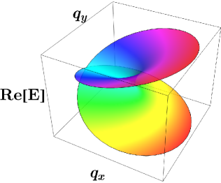
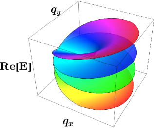
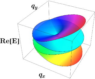
Figure 2: Real parts of the eigenvalues $E$ for the cases of different types EPs when $N=2$: (a) ${\rm Re}[E]$ for a doublet of EP₂’s, where each eigenvalue is doubly degenerate. (b) ${\rm Re}[E]$ for an EP₄, where all different energy eigenvalues coalesce at one singular point. (c) ${\rm Re}[E]$ for an EP₃, for which the eigenvectors are sensitive to how the point of singularity is approached in the Brillouin zone. We choose the EP to be anisotropic. The scaling of $E$ around the EP can take different forms along different directions.

III.3 Odd-order EPs

As we have shown in Sec. II, the sublattice symmetry requires the dispersion near an EP at $E=0$ to scale as $\delta E\sim|\delta\mathbf{q}|^{1/(2p)}$, with $p\in{\mathbb{Z}}^{+}$. In addition, the sublattice symmetry also restricts the ways in which $E\neq 0$ eigenvectors coalesce. These conditions seem to obstruct an odd-order EP. However, through an explicit construction of an EP₃ for the $N=2$ four-band model, we will show that a somewhat anomalous EP₃ can exist. Although the generic case is expected to exhibit a cube-root dispersion around the singularity, a sublattice symmetry forces it to have a square-root-dispersion [37], which is indeed found to be the case here. We also find that the way the eigenvectors coalesce with one another depends on the path chosen to approach the EP₃ (while a regular EP₃ has three eigenvectors collapsing together for any path). The EP₃ here is anomalous and different from the usual scenarios.

Because of the sublattice symmetry, a zero eigenvalue can appear only with an even algebraic multiplicity. Hence, for the $N=2$ case, the existence of an EP₃ with $E=0$ requires that its algebraic multiplicity must be four. The degenerate point is thus an EP₃ plus an accidental zero-energy eigenstate. According to our symmetry analysis, the total dimension of the kernels for $\mathbf{B}(\mathbf{q}_{\ast})$ and $\mathbf{B}(\mathbf{q}_{\ast})$ is $m+n=2$. If $m=2$ and $n=0$, the matrix $\mathbf{B}(\mathbf{q}_{\ast})$ is identically zero, and $\mathbf{B}^{\prime}(\mathbf{q}_{\ast})$ can be brought to a diagonal matrix via a transformation matrix $\mathbf{V}$. Applying the transformation matrix $\textrm{diag}(\mathbf{V},\,\mathbf{V})$ to $H(\mathbf{q}_{\ast})$ then brings it explicitly to a form similar to Eq. (4). Hence, either $(m=2,\,n=0)$ or $(m=0,\,n=2)$ gives a doublet of EP₂’s. An EP₃ can emerge only when $m=n=1$.

Now we look at a specific example. According to Table 1, an EP₃ appears when $V\,H(\mathbf{q}_{\ast})\,V^{-1}=\textrm{diag}\{J_{3}(0),0\}$, and

$$\mathbf{B}(\mathbf{q}_{\ast})=\begin{pmatrix}0&b_{2}\\ 0&0\\ \end{pmatrix},\quad\mathbf{B}^{\prime}(\mathbf{q}_{\ast})=\begin{pmatrix}b^{\prime}_{1}&b^{\prime}_{2}\\ 0&0\\ \end{pmatrix}.$$ (7)

There are two linearly independent eigenvectors at $E=0$, which are proportional to $e_{1}=\left(0,\,0,\,1,\,0\right)^{T}$ and $e_{2}=\left(b^{\prime}_{2},\,-b^{\prime}_{1},\,0,\,0\right)^{T}$, proving that it is not an EP₄. From the Jordan decomposition, we find that $e_{1}$ belongs to a generalized eigenspace of dimension three, such that $e_{1}=H(\mathbf{q}_{\ast})\,\tilde{e}_{2}$ and $\tilde{e}_{2}=H(\mathbf{q}_{\ast})\,\tilde{e}_{3}$, with $\tilde{e}_{2}=\left(1/b^{\prime}_{1},\,0,\,0,\,0\right)^{T}$ and $\tilde{e}_{3}=\left(0,\,0,\,0,\,1/(b_{2}\,b^{\prime}_{1})\right)^{T}$. Hence, this is an EP₃ accidentally coinciding with a zero-energy eigenvector.

To investigate how the symmetry constraints play out in this case, we explicitly show how the eigenvectors behave in the vicinity of this EP₃. As the sublattice symmetry forbids the three eigenvectors folding together, they show an anomalous behaviour, which is in-between the coaslescence features of the eigenvectors of EP₂ and EP₄. This is the reason why the eigenvector-coalescence depends on the path chosen while approaching $\mathbf{q}_{\ast}$. Whenever an EP is anisotropic [47], the eigenvectors indeed exhibit an enhanced path-dependent sensitivity.

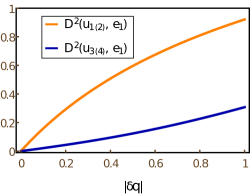
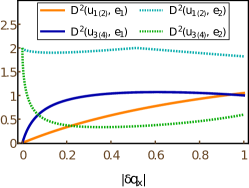
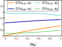
Figure 3: Square of the quantum distance ($D^{2}$) describing how eigenstates coalesce into those at the exceptional points of different orders: (a) $D^{2}(u_{i},e_{1})$ goes to zero at the EP₄ for all $i\in[1,4]$. (b) Approaching the EP₃ along the Path 1 of Sec. III.3 (with $q_{y}=0$), for all $i\in[1,4]$ $D^{2}(u_{i},e_{1})$ goes to zero, while $D^{2}(u_{i},e_{2})$ goes to some nonzero values. (c) When one approaches the EP₃ along the Path 2 of Sec. III.3 (with $q_{x}=0$), $D^{2}(u_{1},e_{1})$ and $D^{2}(u_{2},e_{1})$ go to zero, while $D^{2}(u_{3},e_{j})$ and $D^{2}(u_{3},e_{j})$ remain nonzero for both $j=1,2$.

III.3.1 Path 1

We approach the EP along the $q_{x}$-direction (i.e., $q_{y}=0$ along this path), assuming that all deviations are linear, in which case the expansion looks like

$$\mathbf{B}(\mathbf{q}_{\ast}+\delta q_{x}\,\hat{\boldsymbol{x}}) \simeq\begin{pmatrix}v_{1}(0)\,|\delta q_{x}|&b_{2}\\ v_{3}(0)\,|\delta q_{x}|&v_{4}(0)\,|\delta q_{x}|\\ \end{pmatrix},$$

$$\mathbf{B}^{\prime}(\mathbf{q}_{\ast}+\delta q_{x}\,\hat{\boldsymbol{x}}) \simeq\begin{pmatrix}b^{\prime}_{1}&b^{\prime}_{2}\\ v^{\prime}_{3}(0)\,|\delta q_{x}|&v^{\prime}_{4}(0)\,|\delta q_{x}|\\ \end{pmatrix}.$$ (8)

As before, we implicitly assume that the variables $\{b_{j},\,b^{\prime}_{j}\}$ and $\{v_{j}(0),\,v^{\prime}_{j}(0)\}$ can contain ${\mathcal{O}}(|\delta q_{x}|)$ corrections. The product

$$\mathbf{B}^{\prime}(\mathbf{q}_{\ast}+\delta q_{x}\,\hat{\boldsymbol{x}})\cdot\mathbf{B}(\mathbf{q}_{\ast}+\delta q_{x}\,\hat{\boldsymbol{x}})$$

$$\simeq \begin{pmatrix}[b^{\prime}_{1}\,v_{1}(0)+b^{\prime}_{2}\,v_{3}(0)]\,|\delta q_{x}|&b_{2}\,b^{\prime}_{1}\\ [v_{1}(0)\,v^{\prime}_{3}(0)+v_{3}(0)\,v^{\prime}_{4}(0)]\,|\delta q_{x}|^{2}&b_{2}\,v^{\prime}_{3}(0)\,|\delta q_{x}|\\ \end{pmatrix}$$ (9)

determines the eigenvalue $E^{2}$ and $\chi$ [cf. Eq. (3)]. The two eigenvalues of the above matrix vanish as ${\mathcal{O}}(|\delta q_{x}|)$, while its two eigenvectors approach $(1,0)^{T}$ as $\left(1,\,{\mathcal{O}}(|\delta q_{x}|)\right)^{T}$ (the intermediate steps are shown in Appendix B). Hence, the deviation in dispersion scales as $\delta E\sim\sqrt{|\delta q_{x}|}$. Since the upper component is given by $\psi=i\,\mathbf{B}\,\chi/E$, it vanishes as $\left({\mathcal{O}}(\sqrt{|\delta q_{x}|}),\,{\mathcal{O}}(\sqrt{|\delta q_{x}|})\right)^{T}$. Therefore, all the four eigenvectors coalesce to $e_{1}=(0,\,0,\,1,\,0)^{T}$ at $\mathbf{q}=\mathbf{q}_{\ast}$. In comparison, there is no eigenvector converging to the eigenvector $e_{2}$ at $\mathbf{q}_{\ast}$. Although this EP is of order three, its singularity behaviour along the $q_{x}$-path is similar to a typical EP₄.

III.3.2 Path 2

The eigenvectors exhibit a typical EP₂ behaviour if $v^{\prime}_{3}(\theta)$ and $v^{\prime}_{4}(\theta)$ vanish for some angle $\theta$, which can be obtained by imposing an additional symmetry to these parameters. For convenience, we choose the direction of approach to the EP in this case to be along the $q_{y}$-direction, and set $v^{\prime}_{3}(\pi/2)=v^{\prime}_{4}(\pi/2)=0$. The off-diagonal matrices take the forms:

$$\mathbf{B}(\mathbf{q}_{\ast}+\delta q_{y}\,\hat{\boldsymbol{y}}) \simeq\begin{pmatrix}v_{1}(\pi/2)\,|\delta q_{y}|&b_{2}\\ v_{3}(\pi/2)\,|\delta q_{y}|&v_{4}(\pi/2)\,|\delta q_{y}|\\ \end{pmatrix},$$

$$\mathbf{B}^{\prime}(\mathbf{q}_{\ast}+\delta q_{y}\,\hat{\boldsymbol{y}}) \simeq\begin{pmatrix}b^{\prime}_{1}&b^{\prime}_{2}\\ r^{\prime}_{3}\,|\delta q_{y}|^{2}&r^{\prime}_{4}\,|\delta q_{y}|^{2}\\ \end{pmatrix},$$ (10)

and their product is given by

$$\mathbf{B}^{\prime}(\mathbf{q}_{\ast}+\delta q_{y}\,\hat{\boldsymbol{y}})\cdot\mathbf{B}(\mathbf{q}_{\ast}+\delta q_{y}\,\hat{\boldsymbol{y}})$$

$$\simeq \begin{pmatrix}\left[b^{\prime}_{1}\,v_{1}(\pi/2)+b^{\prime}_{2}\,v_{3}(\pi/2)\right]|\delta q_{y}|&b_{2}\,b^{\prime}_{1}\\ \left[v_{1}(\pi/2)\,r^{\prime}_{3}+v_{3}(\pi/2)\,r^{\prime}_{4}\right]|\delta q_{y}|^{3}&b_{2}\,r^{\prime}_{3}\,|\delta q_{y}|^{2}\\ \end{pmatrix}.$$ (11)

One of its eigenvalues of the product matrix vanishes as $\lambda_{1}={\mathcal{O}}(|\delta q_{y}|)$, while the other vanishes as $\lambda_{2}={\mathcal{O}}(|\delta q_{y}|^{2})$ (the derivations are shown in Appendix B). Note that this gives a different scaling for the dispersion around the EP, compared to the Path 1. The two eigenvectors of $\mathbf{B}^{\prime}\cdot\mathbf{B}$ behave as $\chi_{1}\simeq(1,\,{\mathcal{O}}(|\delta q_{y}|^{2}))^{T}$ and $\chi_{2}\simeq\left(1,{\mathcal{O}}(|\delta q_{y}|)\right)^{T}$, respectively. The corresponding upper components (obtained from the relations $\psi_{a}=i\,\mathbf{B}\,\chi_{a}/E$, with $a\in\{1,2\}$) thus scale as $\psi_{1}\sim\left({\mathcal{O}}(\sqrt{|\delta q_{y}|}),{\mathcal{O}}(\sqrt{|\delta q_{y}|})\right)^{T}$ and $\psi_{2}\sim\left({\mathcal{O}}(1),{\mathcal{O}}(1)\right)^{T}$, respectively. In this situation, the two eigenvectors $(\pm\psi^{T}_{1},\chi^{T}_{1})$ converge to $e_{1}^{T}$, while the other two eigenvectors $(\pm\psi^{T}_{2},\chi^{T}_{2})$ go to two other linearly-independent vectors, which we denote as $e_{3}^{T}$ and $e_{4}^{T}$. Hence, along this path, the eigenvectors behave as a single eigenvector of an EP₂ plus two linearly-independent accidental zero-energy eigenvectors.

IV Irregular subspace topology of the EPs

In this section, we will formulate a way to quantitatively characterize the overlap of eigenvectors, following which we will illustrate the origin of the anomalous behaviour of the odd-order EPs under sublattice symmetry. The conclusion that comes out of this set-up is that eigenvector-coalescence is not actually a point-like property of the EP itself, but it depends on how the Hamiltonian looks like in its neighborhood. In fact, we will see that for our example of $N=2$, the EP₃ under sublattice symmetry can in fact be understood as the point at which the parameter spaces of EP₄ and EP₂ intersect. This feature comes from the subspace topology of $\mathcal{EP}_{n}$, as a subspace of all $4\times 4$ matrices $M_{4}(\mathbb{C})$.

When analyzing the coalescence of eigenvectors, it can be ambiguous if we directly compare them, because eigenvectors are equivalent upto phases. In order to characterize unambiguously how the states coalesce near regular EPs and mixed-type EPs, it is most convenient to introduce the quantum distance $D$ [48], such that

$$D^{2}(u,u^{\prime}) =\underset{\{\alpha,\beta\}\in\,\mathbb{R}}{\textrm{inf }}\,||\,u\,e^{i\,\alpha}-u^{\prime}\,e^{i\,\beta}||^{2}$$

$$=2-2\,|\langle u\,|\,u^{\prime}\rangle|\,.$$ (12)

Clearly, $D^{2}(u,u^{\prime})$ is invariant under $U(1)\times U(1)$ transformations, i.e., under the change of the phases of $u$ and $u^{\prime}$. Here the states are normalized as $\langle u\,|\,u\rangle=\langle u^{\prime}\,|\,u^{\prime}\rangle=1$, and $||\cdot||$ is the usual norm $\sqrt{\langle\cdot|\cdot\rangle}$ of a quantum state. Using $u^{\prime}$ to denote the eigenvectors at the EP at $\mathbf{q}=\mathbf{q}_{\ast}$, and $u$ to denote the states away from $\mathbf{q}_{\ast}$, $D$ is a function of $(\mathbf{q}-\mathbf{q}_{\ast})$. $D^{2}$ is positive-definite, and vanishes only when $u$ and $u^{\prime}$ differ by a phase (i.e., when $u$ and $u^{\prime}$ denote the same quantum state). Hence, $D^{2}(u,e_{j})$ can be used to describe unambiguously how the eigenvectors are approaching their target eigenvectors at the EP.

Since the eigenstates $e_{j}$’s at the EP (i.e., at $E=0$) are invariant under the sublattice symmetry, the two nondegenerate eigenstates $(\pm\psi,\chi)$, related by the sublattice symmetry, have the same $D^{2}$ value with $e_{j}$. In Fig. 3, we show how the eigenvectors approach the ones at the EPs, as $\mathbf{q}$ approaches $\mathbf{q}_{\ast}$. In all the cases, the four nondegenerate states fall into two classes: each corresponding to a sublattice symmetry-related pair. Let us denote the two pairs of eigenvectors as $\{u_{1},u_{2}\}$ and $\{u_{3},u_{4}\}$. For the EP₄, $D^{2}$ is computed from $e_{1}$ (which is the sole linearly-independent eigenvector right at the EP) and each of the four nondegenerate eigenvectors, and it goes to zero as we approach the EP₄. However, things are more complicated for the EP₃, and in fact the behaviour of $D^{2}$ corroborates the results obtained in Sec. III.3. Approaching the EP along the Path 1 of Sec. III.3 (with $q_{y}=0$), for all $i\in[1,4]$, $D^{2}(u_{i},e_{1})$ goes to zero, while $D^{2}(u_{i},e_{2})$ remains nonvanishing. On the other hand, if one approaches the EP along the Path 2 (with $q_{x}=0$), $D^{2}(u_{1},e_{1})$ and $D^{2}(u_{2},e_{1})$ go to zero, while $D^{2}(u_{3},e_{j})$ and $D^{2}(u_{3},e_{j})$ remain nonzero for both $j=1$ and $j=2$.

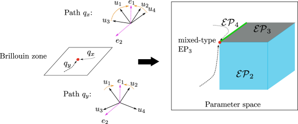
Figure 4: Schematic depiction of the location of a mixed-type EP₃ in the parameter space of a non-Hermitian matrix. The white (uncoloured) region in the parameter space represents matrices with nondegenerate eigenvalues. They are dense and their parameter space has the highest dimensionality. In the absence of any symmetry, the dimension of the $\mathcal{EP}_{n}$ space decreases as $n$ increases. The mixed-type EP₃ appears as the intersection point of the $\mathcal{EP}_{2}$ (light blue cube), $\mathcal{EP}_{3}$ (gray surface), and $\mathcal{EP}_{4}$ (green line). When the sublattice symmetry is imposed, the regular $\mathcal{EP}_{3}$ surface (gray region) is forbidden, and the mixed-type EP₃ can be approached only via the neighbourhood of either $\mathcal{EP}_{4}$ (dotted line) or $\mathcal{EP}_{2}$ (dashed line). This leads to two different ways of eigenvector-coalescence, which are shown by the collapse of directed arrows against “Path $q_{x}$” and “Path $q_{y}$” (corresponding to Path 1 and Path 2 of Sec. III.3, respectively).

The anomalous behaviour of the eigenvectors near the EP₃ can be explained by its mixed nature. This is a very special property of a Jordan decomposition when the diagonal of a Jordan block coincides with some other eigenvalue(s). An EP with such a Jordan block is qualitatively different from an EP whose Jordan block has a nonzero gap with other eigenvalues. We denote the latter as regular EPs. The space $\mathcal{EP}_{3}$ comprises two sets, namely, the set $U_{1}$ of regular EP₃ and the set $U_{2}$ of mixed-nature EP₃.

To illustrate the possible structures around an EP₃, we consider a $4\times 4$ matrix $M$ with no particular symmetry. Such a matrix has a $16$ (complex) dimensional parameter space $M_{4}(\mathbb{C})$. The most common matrices in this space are those which are the non-singular ones featuring nondegenerate eigenvalues. The EPs are represented by matrices with singularity, and they form lower-dimensional subspaces of $M_{4}(\mathbb{C})$. The dimension of the parameter space $\mathcal{EP}_{n}$ decreases as $n$ becomes larger (see Appendix C). For an EP₃ with Jordan decomposition $M\big{|}_{\rm{EP}_{3}}=\mathrm{diag}\{J_{3}(0),\,0\}$, one can easily verify that, within $\mathcal{EP}_{2}$, there is a sequence of points whose limit is $M\big{|}_{\rm{EP}_{3}}$:

$$\lim\limits_{\epsilon\to 0} \left[M(\epsilon)\big{|}_{\rm{EP}_{2}}=\begin{pmatrix}0&1&0&0\\ 0&0&1&0\\ 0&0&\epsilon&0\\ 0&0&0&2\epsilon\\ \end{pmatrix}\in\mathcal{EP}_{2}\right]=M\big{|}_{\rm{EP}_{3}}$$

$$= \begin{pmatrix}0&1&0&0\\ 0&0&1&0\\ 0&0&0&0\\ 0&0&0&0\\ \end{pmatrix}\in U_{2}\subset\mathcal{EP}_{3}\,.$$ (13)

This implies that, in any neighbourhood of $M\big{|}_{\rm{EP}_{3}}$, we can always find points belonging to $\mathcal{EP}_{2}$. In particular, when the matrices representing nondegenerate eigenvalues are close enough to the matrices representing EP₂’s, two of the four eigenvectors of our non-Hermitian Hamiltonian should also come close to each other (see Fig. 4).

In addition to the above limit, we can find another limit by tuning the parameters of the matrix containing the Jordan block of the EP₃, such that the EP₃ of $M\big{|}_{\rm{EP}_{3}}$ is now a limiting point of an $\mathcal{EP}_{4}$. This can be seen from

$$\lim\limits_{\epsilon\to 0} \left[M(\epsilon)\big{|}_{\rm{EP}_{4}}=\begin{pmatrix}0&1&0&0\\ 0&0&1&0\\ 0&0&0&\epsilon\\ 0&0&0&0\\ \end{pmatrix}\in\mathcal{EP}_{4}\right]=M\big{|}_{\rm{EP}_{3}}$$

$$= \begin{pmatrix}0&1&0&0\\ 0&0&1&0\\ 0&0&0&0\\ 0&0&0&0\\ \end{pmatrix}\in U_{2}\subset\mathcal{EP}_{3}\,.$$ (14)

This result is much more counter-intuitive than the coincidence with the EP₂ case, because $\mathcal{EP}_{4}$ has a lower dimension than $\mathcal{EP}_{3}$, and the region $M(\epsilon)\big{|}_{\rm{EP}_{4}}$ in the neighbourhood of $M\big{|}_{\rm{EP}_{3}}$ is usually very small. However, the neighbourhood of $\mathcal{EP}_{4}$ comprising all matrices representing nondegenerate eigenvalues is not small. These matrices then can have a large overlap with the nondegenerate neighbourhood of $M\big{|}_{\rm{EP}_{3}}$. As a result, all paths through this intersecting region will show a behaviour characteristic of a four-fold eigenvector-coalescence.

The arguments above show that a mixed-type EP can appear as a common limit point of lower- and higher-order EPs, which implies that such an exceptional degeneracy cannot form a closed subspace in $M_{4}(\mathbb{C})$ by simply combining certain higher-order EPs. This anomalous behaviour of the odd-order EPs is absent in Hermitian systems. In the parameter space of a Hermitian matrix $H_{\text{herm}}$, if we denote the space with an $n$-fold degenerate eigenvalue $E$ as $\mathcal{HD}_{n}(E)$, the space $\cup_{n\geq m}\mathcal{HD}_{n}(E)$ is given by the zeros of the resultants ($R$) or discriminants ($\mathcal{D}$), i.e., by $R(E)=0$ [38] or $\mathcal{D}[H_{\text{herm}}(E)]=0$ [40]. These equations involve continuous functions in $M_{4}(\mathbb{C})$, and hence their solutions constitute a closed subspace of $M_{4}(\mathbb{C})$. This means that the limit of a series Hermitian degeneracy $\mathcal{HD}_{n}$ can only end in some $\mathcal{HD}_{m}$ ($m\geq n$). As a result, only higher-order degeneracy can be the limit of a lower-order degeneracy, but not the other way around. Therefore, for Hermitian matrices, there is no mixed-type degeneracy.

In summary, the enhanced eigenvector sensitivity can be understood intuitively in the following way (see also Fig. 4). The different directions of approaching $\mathbf{q}_{\ast}$ in the Brillouin zone can be mapped to approaching the EP₃ through different tracks in the space of matrices representing nondegenerate eigenvalues. Due to the sublattice symmetry, it is forbidden to approach the EP₃ through the neighbourhood of the matrices representing a regular EP₃. Consequently, the sublattice symmetry-restricted EP₃ can only be reached through the neighbourhoods of $\mathcal{EP}_{2}$ and $\mathcal{EP}_{4}$. Of course in those neighbourhoods, either two or four eigenvectors coalesce together, leading to the anomalous behaviour of the eigenvectors of the EP₃.

V Lattice realizations and expectations for generic $N$-values

Examples of fermionic Hamiltonians with sublattice symmetry include solvable spin liquid models, such as the Kitaev spin liquid [44, 12, 17] (corresponding to $N=1$), and the Yao-Lee $SU(2)$ spin liquid [45] (corresponding to $N=3$). The $N=2$ model studied in this paper can be embedded in the Yao-Lee model. There, the low-energy physics is described by $N=3$ flavours of Majorana fermion operators, with the Hamiltonian consisting of only nearest-neighbour hoppings amongst fermions of the same flavour. In order to produce the higher-order degeneracies discussed in this paper, we need to introduce terms which couple different flavours [thus breaking the $SU(N)$ symmetry] – these can be generated by terms $\sigma_{\alpha,i}\,\tau^{x}_{i}\,\tau^{x}_{j}\,\sigma_{\beta,j}$ (with $i\neq j$) in terms of the original spin operators. The details have been outlined in Appendix E.

Setting $N=3$, one can get EPs up to sixth order, which is then expected to display a richer eigenvector sensitivity. For this case, an EP₅ can exist where a five-dimensional Jordan block becomes degenerate with another band. Near this EP₅, the coalescence of eigenvectors can be four-fold or six-fold. Moreover, since two-fold coalescence is also permitted by the sublattice symmetry, there exists paths along which the eigenvectors collapse like they do in the vicinity of an EP₂. Consequently, such an EP₅ has a higher degree of eigenvector sensitivity, making it possible to have more knobs to tune quantum states.

For a generic value of $N$, in order to obtain an $N$-fold compound EP₂, or a highest-order simple EP_2N, the algebraic conditions are simply obtained by replacing the expressions for $N=2$ by the appropriate $N$-value. More specifically, the $N$-fold EP₂ is $SU(N)$-invariant, and is obtained by choosing $\mathbf{B}$ as a diagonal matrix vanishing at $\mathbf{q}_{\ast}$, while $\mathbf{B}^{\prime}(\mathbf{q}_{\ast})$ remains nonzero. As for EP_2N, we need $\dim(\ker\mathbf{B})+\dim(\ker\mathbf{B}^{\prime})=1$ for generic $N$ as well. Additionally, in order to ensure that all the $2N$ linearly-independent eigenvectors coalesce to a single one, we need to impose the condition $\mathbf{B}\cdot\mathbf{B}^{\prime}\sim J_{2N}(0)$, which can alternatively be represented as $\ker(\mathbf{B}\cdot\mathbf{B}^{\prime})^{m}=\mathrm{im}(\mathbf{B}\cdot\mathbf{B}^{\prime})^{2N-m}$ (with $0<m<2N$). For EPs with orders between $2$ and $2N$, the analysis becomes more complicated. Mixed-type odd-order EPs will exist at $E=0$, analogous to the EP₃ of the $N=2$ case that we have explicitly studied. Although the dimensions of the kernels can be worked out in a way similar to that shown in Table 1, the image and kernel relations need to be figured out on a case-by-case basis, and closed-form expressions for the eigenvectors might involve extremely complicated calculations. Nevertheless, the generic topological relations between higher-order EPs remain valid.

VI Summary and outlook

In this paper, we have explored the emergence of higher-order EPs in two-dimensional four-band non-Hermitian systems, with a sublattice symmetry. Such systems are relevant to non-Hermitian extensions of solvable spin liquid models. The sublattice symmetry forces the eigenvalues to appear in pairs of $\{E,-E\}$, and the dispersion around an EP is restricted to be an even root of the deviation in the momentum space. We have explicitly computed how the eigenvectors collapse at an EP, and found an anomalous behaviour for odd-order EPs. Based on the analytical solvability of a four-band system, we have shown that the collapse of the eigenvectors depends on the specific path of approaching an EP₃. The behaviour is anomalous in the sense that it is in contradiction with the intuition that $n$ eigenvectors always coalesce together at an EP_n. In fact, the number of collapsing eigenvectors for a mixed-type odd-order EP is an even number smaller or greater than $n$, which is caused by the presence of the sublattice symmetry. Intuitively, this unconventional feature can be understood from the fact that there is a restriction in the parameter space of EP₃ due to the sublattice symmetry, and this unusual EP₃ can be approached only via the neighbourhoods of EP₂’s and EP₄’s.

Using the notion of a quantum distance, we have further explored the behaviour of the eigenvectors near the mixed-type EP₃. We have found that the eigenvectors do not necessarily converge to those of a regular EP₃, especially when we are approaching it from a neighbourhood of $\mathcal{EP}_{2}$. The quantum distance to the eigenvectors at the mixed-type EP₃ can change abruptly if we slightly perturb the approaching process. It is already known that the non-unitary evolution under a non-Hermitian Hamiltonian leads to a shorter quantum distance [49, 50], which can play a role in state preparation. Hence, we expect that the anomalous behaviour near higher-order EPs will significantly enhance this effect, and lead to novel applications exploiting the features we have discovered through our analysis.

The enhanced eigenvector sensitivity for the mixed-type EP₃s is a reminiscence of generic counter-intuitive features specific to non-Hermitian systems (i.e., these are absent in the corresponding Hermitian counterparts). A very well-known example is the non-Hermitian skin effect [51, 52, 53, 54, 55, 56, 57, 58, 59], where a very small change in the boundary conditions brings about remarkable modifications to the spectrum. The mixed nature of the odd-order EPs also generalizes the notion of the recently-studied non-defective EPs [60], where a Hermitian degeneracy mixes with the usual EP₂.

A promising future research direction is to explore analogous unconventional EPs in three-dimensional systems with appropriate symmetry constraints. The extended dimensionality is expected to provide a richer parameter space for the characterization of generic EPs [61]. Another significant direction is to investigate the role of the higher-order EPs, especially the odd-order ones with anomalous behaviour, in designing non-Hermitian topological sensors [32]. Due to higher-order singular behaviour near a regularly behaved higher-order EP, the sensors based on such EPs are expected to show greater sensitivity than an EP₂, and the existence of mixed-type EPs may enable us to tune the sensitivity by tuning the parameter space [62].

Appendix A Exceptional degeneracy under sublattice symmetry

When a symmetry is imposed, the standard method for obtaining the EP parameter space (see Appendix C) can be very complicated to employ in practice. Therefore, we adopt a more direct way to find the EP parameter space under sublattice symmetry, which employs the algebraic connections between $\mathbf{B}$ and $\mathbf{B}^{\prime}$ as linear transformation operators. In this appendix, we demonstrate this method for the $N=2$ case, where we can obtain closed-form expressions. We use $\mathbb{C}^{\times}$ to represent the set of all complex numbers $z\neq 0$. We also introduce the notation $\mathcal{J}_{n}$ to denote the set of nondegenerate matrices commuting with the Jordan block $J_{n}$. In fact, $\mathcal{J}_{n}$ is given by all upper-triangular translational-invariant matrices [41] .

To get the $SU(2)$-invariant doublet of EP₂’s, the Hamiltonian is determined by $\mathbf{B}$ or $\mathbf{B}^{\prime}$ with a second-order EP. Hence, the corresponding parameter space $\mathcal{EP}_{2}$ is given by $GL(2)/\mathcal{J}_{2}$.

For $\mathcal{EP}_{4}$, we notice that $\dim(\ker\mathbf{B})+\dim(\ker\mathbf{B}^{\prime})=1$, according to the discussions in the main text. Assuming that $\dim(\ker\mathbf{B})=1,\dim(\ker\mathbf{B}^{\prime})=0$, without any loss of generality, $\mathbf{B}^{\prime}$ is invertible. As we have shown in Sec. III.3, the matrix $\mathbf{B}\cdot\mathbf{B}^{\prime}$ must be similar to $J_{2}(0)$, which means $\mathbf{B}\cdot\mathbf{B}^{\prime}\cdot\mathbf{B}\cdot\mathbf{B}^{\prime}=\mathbf{B}\cdot\mathbf{B}^{\prime}\cdot\mathbf{B}=0$. There can be two scenarios according to whether $\mathbf{B}$ is diagonalizable or non-diagonalizable:

1. When $\mathbf{B}$ is diagonalizable, let the eigenvectors of $\mathbf{B}$ be $\chi_{1}$ and $\chi_{2}$. We choose $\chi_{1}\in\ker\mathbf{B}$. In order to have $\mathbf{B}\cdot\mathbf{B}^{\prime}\cdot\mathbf{B}=0$, it is enough to have $\left(\mathbf{B}\cdot\mathbf{B}^{\prime}\cdot\mathbf{B}\right)\chi_{2}=0$. Since $\chi_{2}$ is an eigenvector with a nonzero eigenvalue, this is equivalent to $\left(\mathbf{B}\cdot\mathbf{B}^{\prime}\right)\chi_{2}=0$, implying that $\mathbf{B}^{\prime}\,\chi_{2}\in\ker\mathbf{B}$. Switching to the basis formed by $\chi_{1}$ and $\chi_{2}$, we get

   $$\mathbf{B}^{\prime}=\begin{pmatrix}b^{\prime}_{1}&b^{\prime}_{2}\\ b^{\prime}_{3}&0\\ \end{pmatrix}\textrm{ when }\mathbf{B}=\begin{pmatrix}0&0\\ 0&b_{4}\\ \end{pmatrix},$$ (15)

   with $b_{4}$ denoting the eigenvalue corresponding to $\chi_{2}$. In order to ensure that $\mathbf{B}^{\prime}$ invertible, we need $b^{\prime}_{2}\,b^{\prime}_{3}\neq 0$.

2. When $\mathbf{B}$ is not diagonalizable, it is equal to $J_{2}(0)$ in a basis formed by two linearly independent vectors $\chi_{1}$ and $\chi_{2}$, still with $\chi_{1}\in\ker\mathbf{B}$. Here also, we only need to have $\left(\mathbf{B}\cdot\mathbf{B}^{\prime}\cdot\mathbf{B}\right)\chi_{2}=0$, which is now equivalent to $\left(\mathbf{B}\cdot\mathbf{B}^{\prime}\right)\chi_{1}=0$. This tells us that $\mathbf{B}^{\prime}\,\chi_{1}\propto\chi_{1}$, i.e., $\chi_{1}$ is also an eigenvector of $\mathbf{B}^{\prime}$. Switching to the basis formed by $\chi_{1}$ and $\chi_{2}$, we get

   $$\mathbf{B}^{\prime}=\begin{pmatrix}b^{\prime}_{1}&b^{\prime}_{2}\\ 0&b^{\prime}_{4}\\ \end{pmatrix}\text{ when }\mathbf{B}=\begin{pmatrix}0&1\\ 0&0\\ \end{pmatrix}.$$ (16)

   The invertibility of $\mathbf{B}^{\prime}$ requires that $b^{\prime}_{1}\,b^{\prime}_{4}\neq 0$. Therefore, we find that the parameter space $\mathcal{EP}_{4}$ comprises two sets: $\mathbb{Z}_{2}\times\mathbb{C}\times(\mathbb{C}^{\times})^{3}\times GL(2)/(\mathbb{C}^{\times})^{2}$ and $\mathbb{Z}_{2}\times\mathbb{C}\times(\mathbb{C}^{\times})^{2}\times GL(2)/\mathcal{J}_{2}$. The $\mathbb{Z}_{2}$ part in either set comes from the symmetry under $\mathbf{B}\leftrightarrow\mathbf{B}^{\prime}$.

The space $\mathcal{EP}_{3}$, as shown in Sec. III.3, is restricted to obey $\dim(\ker\mathbf{B})=\dim(\ker\mathbf{B}^{\prime})=1$. Basic linear algebra then tells us that their corresponding image dimensions are also equal to one, i.e., $\dim(\textrm{im}\,\mathbf{B})=\dim(\textrm{im}\,\mathbf{B}^{\prime})=1$. Let the corresponding eigenvectors be $\chi_{1}$ and $\psi_{1}$, such that $\mathbf{B}\,\chi_{1}=0$ and $\mathbf{B}^{\prime}\,\psi_{1}=0$. It is straightforward to verify that $(0,\chi_{1}^{T})^{T}$ and $(\psi_{1}^{T},0)^{T}$ are eigenvectors of $H$. We assume that $(0,\,\chi_{1}^{T})^{T}$ belongs to a generalized eigenspace of dimension three. Hence, there exists a vector $(\psi_{2},\chi_{2})$ such that $H\,(\psi_{2}^{T},\chi_{2}^{T})^{T}=(0,\chi_{1}^{T})^{T}$. This implies $\chi_{2}\in\ker\mathbf{B}$ and $-i\,\mathbf{B}^{\prime}\psi_{2}=\chi_{1}$, requiring $\textrm{im}\,\mathbf{B}^{\prime}=\ker\mathbf{B}$. We can choose $\psi_{2}$ to be in the subspace complementary to that of $\psi_{1}$ (i.e., $\psi_{2}\in\{\mathbb{C}^{2}-(\ker\mathbf{B}^{\prime})\}$) and set $\chi_{2}=0$. In order to form a three-dimensional generalized eigenspace, we need a third linearly-independent vector $(\psi_{3},\chi_{3})$, such that $H\,(\psi_{3}^{T},\chi_{3}^{T})^{T}=(\psi_{2}^{T},0)^{T}$. From this relation, we have $\psi_{3}\in\ker\mathbf{B}^{\prime}$ and $\textrm{im}\,\mathbf{B}\neq\ker\mathbf{B}^{\prime}$, which enforces the condition $\psi_{2}\in\textrm{im}\,\mathbf{B}$ – therefore we can choose $\psi_{3}=0$ and $\chi_{3}\in(\ker\mathbf{B})_{\perp}$. One can verify that the four vectors – $(0,\,\chi_{1}^{T})^{T}$, $(\psi_{1}^{T},0)^{T}$, $(\psi_{2}^{T},0)^{T}$, and $(0,\chi_{3}^{T})^{T}$ – that we have just constructed, are linearly-independent. To summarize, once the matrix $\mathbf{B}$ is fixed, the image of $\mathbf{B}^{\prime}$ also gets fixed, and $\ker\mathbf{B}^{\prime}$ must be different from $\textrm{im}\,\mathbf{B}$. Since $\dim(\ker\mathbf{B}^{\prime})=1$, the matrix $\mathbf{B}^{\prime}$ is determined by $\mathbf{B}$ up to a nonzero vector (characterizing the ratio between the first and second columns of $\mathbf{B}^{\prime}$). The matrix $\mathbf{B}$ can be built from two linearly dependent row vectors:

$$\mathbf{B}=\begin{pmatrix}p_{1}\,u_{1}&p_{1}\,u_{2}\\ p_{2}\,u_{1}&p_{2}\,u_{2}\end{pmatrix},$$ (17)

because its kernel is one-dimensional. Here at least one of $p_{1}$ and $p_{2}$ is nonzero and so are $u_{1},u_{2}$. The kernel of $\mathbf{B}$ is generated by the vector $(u_{2},\,-u_{1})^{T}$, and its image is generated by $(p_{1},\,p_{2})^{T}$. According to the relations between $\mathbf{B}$ and $\mathbf{B}^{\prime}$, we have

$$\mathbf{B}^{\prime}=\begin{pmatrix}p^{\prime}_{2}\,u_{2}&-p^{\prime}_{1}\,u_{2}\\ -p^{\prime}_{2}\,u_{1}&p^{\prime}_{1}\,u_{1}\end{pmatrix},$$ (18)

where $(p^{\prime}_{1},p^{\prime}_{2})$ is not collinear with $(p_{1},p_{2})$. We observe that all the pairs $(u_{1},\,u_{2})$, $(p_{1},\,p_{2})$, and $(p^{\prime}_{1},\,p^{\prime}_{2})$ exclude the origin $(0,0)$. Since $\mathbf{B}$ is invariant under the transformations $u_{i}\to z\,u_{i}$, $p_{i}\to p^{\prime}_{i}/z$, and $p^{\prime}_{i}\to p^{\prime}_{i}/z$, its parameter space is represented by $\mathbb{C}^{2\times}\times\mathbb{C}^{2\times}\times(\mathbb{C}^{2}-\mathbb{C})/\mathbb{C}^{\times}$. This leads to the final result that $\mathcal{EP}_{3}$ is given by $\mathbb{Z}_{2}\times\mathbb{C}^{2\times}\times\mathbb{C}^{2\times}\times(\mathbb{C}^{2}-\mathbb{C})/\mathbb{C}^{\times}$.

Appendix B Solutions for eigenvectors near an EP

In this appendix, we work out the explicit expressions for the eigenvalues and eigenvectors near the EP₄ and EP₃ studied in Sec. III. Near the EP₄, the off-diagonal submatrices of the Hamiltonian take the forms:

$$\mathbf{B}(\mathbf{q}_{\ast}+\delta\mathbf{q}) \simeq\begin{pmatrix}v_{1}(\theta)\,|\delta\mathbf{q}|&b_{2}\\ 0&v_{4}(\theta)\,|\delta\mathbf{q}|\\ \end{pmatrix},$$

$$\mathbf{B}^{\prime}(\mathbf{q}_{\ast}+\delta\mathbf{q}) \simeq\begin{pmatrix}b^{\prime}_{1}&0\\ v^{\prime}_{3}(\theta)\,|\delta\mathbf{q}|&b^{\prime}_{4}\\ \end{pmatrix},$$ (19)

to leading order in the powers of $|\delta\mathbf{q}|$. Their product matrix is given by

$$\mathbf{B}^{\prime}(\mathbf{q}_{\ast}+\delta\mathbf{q})\cdot\mathbf{B}(\mathbf{q}_{\ast}+\delta\mathbf{q})$$

$$\simeq \begin{pmatrix}b^{\prime}_{1}\,v_{1}(\theta)\,|\delta\mathbf{q}|&b_{2}\,b^{\prime}_{1}\\ v_{1}(\theta)\,v^{\prime}_{3}(\theta)\,|\delta\mathbf{q}|^{2}&\left[b_{2}\,v^{\prime}_{3}(\theta)+v_{4}(\theta)\,b^{\prime}_{4}\right]|\delta\mathbf{q}|\\ \end{pmatrix},$$ (20)

with eigenvalues

$$\lambda_{a}=\frac{1}{2}\left[b^{\prime}_{1}\,v_{1}+b_{2}\,v^{\prime}_{3}+b^{\prime}_{4}\,v_{4}+(-1)^{a+1}\sqrt{(b^{\prime}_{1}\,v_{1}+b_{2}\,v^{\prime}_{3}+b^{\prime}_{4}\,v_{4})^{2}-4\,b^{\prime}_{4}\,v_{4}\,b^{\prime}_{1}\,v_{1}}\right]|\delta\mathbf{q}|\,,\text{ with }a\in\{1,2\}.$$ (21)

The four eigenvalues $E$ of the Hamiltonian are therefore given by $\pm\sqrt{\lambda_{1}}$ and $\pm\sqrt{\lambda_{2}}$. The (unnormalized) eigenvectors of $\mathbf{B}^{\prime}\cdot\mathbf{B}$ are

$$\chi^{T}_{a}=\left(1,-\frac{2\,v_{1}\,v^{\prime}_{3}\,|\delta\mathbf{q}|}{b_{2}\,v^{\prime}_{3}+b^{\prime}_{4}\,v_{4}-b^{\prime}_{1}\,v_{1}+(-1)^{a}\sqrt{(b_{2}\,v^{\prime}_{3}+b^{\prime}_{4}\,v_{4}-b^{\prime}_{1}\,v_{1})^{2}+4\,b^{\prime}_{1}\,v_{1}\,b_{2}\,v^{\prime}_{3}}}\right)\simeq\left(1,\,{\mathcal{O}}(|\delta\mathbf{q}|)\right),$$ (22)

and hence are seen to converge to $(1,0)$ at the EP. Using the relation $\psi_{a}=i\,\mathbf{B}\,\chi_{a}/E$ for $E\neq 0$, we deduce that $\psi^{T}_{a}\simeq\bigg{(}{\mathcal{O}}\big{(}|\delta\mathbf{q}|^{1/2}\big{)},\,{\mathcal{O}}\big{(}|\delta\mathbf{q}|^{3/2}\big{)}\bigg{)}$, giving the four eigenvectors of the Hamiltonian as $(\pm\psi_{a}^{T},\chi_{a}^{T})^{T}$. Clearly, these four vectors collapse to $e_{1}=(0,0,1,0)^{T}$, as described in the main text.

As for the EP₃, since the exact expression is quite complicated, we only show the leading order terms. For Path 1, where all deviations from the EP are linear, we have

$$\mathbf{B}(\mathbf{q}_{\ast}+\delta\mathbf{q}) \simeq\begin{pmatrix}v_{1}(0)\,|\delta q_{x}|&b_{2}\\ v_{3}(0)\,|\delta q_{x}|&v_{4}(0)\,|\delta q_{x}|\\ \end{pmatrix},$$

$$\mathbf{B}^{\prime}(\mathbf{q}_{\ast}+\delta\mathbf{q}) \simeq\begin{pmatrix}b^{\prime}_{1}&b^{\prime}_{2}\\ v^{\prime}_{3}(0)\,|\delta q_{x}|&v^{\prime}_{4}(0)\,|\delta q_{x}|\\ \end{pmatrix},$$ (23)

leading to

$$\mathbf{B}^{\prime}(\mathbf{q}_{\ast}+\delta\mathbf{q})\cdot\mathbf{B}(\mathbf{q}_{\ast}+\delta\mathbf{q})$$

$$\simeq \begin{pmatrix}[b^{\prime}_{1}v_{1}(0)+b^{\prime}_{2}v_{3}(0)]\,|\delta q_{x}|&b_{2}\,b^{\prime}_{1}\\ [v_{1}(0)\,v^{\prime}_{3}(0)+v_{3}(0)\,v^{\prime}_{4}(0)]\,|\delta q_{x}|^{2}&b_{2}\,v^{\prime}_{3}(0)\,|\delta q_{x}|\\ \end{pmatrix}$$

$$= p_{2}\begin{pmatrix}p_{1}\,|\delta q_{x}|&1\\ p_{3}\,|\delta q_{x}|^{2}&p_{4}\,|\delta q_{x}|\end{pmatrix}.$$ (24)

Since the eigenvalues of the product matrix are

$$\lambda_{a}\simeq \frac{p_{2}}{2}\left[p_{1}+p_{4}+(-1)^{a}\,\sqrt{(p_{1}-p_{2})^{2}+4\,p_{3}}\right]|\delta q_{x}|$$

$$+{\mathcal{O}}(|\delta q_{x}|^{2})\text{ with }a\in\{1,2\}\,,$$ (25)

the eigenvalues of the Hamiltonian are of ${\mathcal{O}}(\sqrt{|\delta q_{x}|})$. The corresponding eigenvectors are given by

$$\chi_{a}\simeq \left(1,\,\frac{2\,p_{3}\,|\delta q_{x}|}{p_{1}-p_{4}+(-1)^{a}\,\sqrt{(p_{1}-p_{2})^{2}+4\,p_{3}}}\right)^{T}$$

$$\simeq \Big{(}1,\,{\mathcal{O}}(|\delta q_{x}|)\Big{)}^{T}.$$ (26)

According to the relation $\psi_{a}=i\,\mathbf{B}\,\chi_{a}/E$ [with $i\,\mathbf{B}\,\chi_{a}\simeq\Big{(}{\mathcal{O}}(|\delta q_{x}|),\,{\mathcal{O}}(|\delta q_{x}|)\Big{)}^{T}$], each $\psi_{a}$ vanishes as $|\delta q_{x}|\to 0$. Overall, the four eigenvectors $(\pm\psi_{a}^{T},\chi_{a}^{T})^{T}$ are seen to collapse to $e_{1}=(0,\,0,\,1,\,0)^{T}$, resulting in the EP₃ behaving as a typical EP₄, as far as the eigenvector-coalescence is concerned.

When we consider Path 2 for approaching the EP₃, the off-diagonal matrices are given by

$$\mathbf{B}(\mathbf{q}_{\ast}+\delta\mathbf{q})\simeq\begin{pmatrix}v_{1}\,|\delta q_{y}|&b_{2}\\ v_{3}\,|\delta q_{y}|&v_{4}\,|\delta q_{y}|\\ \end{pmatrix}$$

and $$\mathbf{B}^{\prime}(\mathbf{q}_{\ast}+\delta\mathbf{q})\simeq\begin{pmatrix}b^{\prime}_{1}&b^{\prime}_{2}\\ r^{\prime}_{3}\,|\delta q_{y}|^{2}&r^{\prime}_{4}\,|\delta q_{y}|^{2}\\ \end{pmatrix},$$ (27)

leading to

$$\mathbf{B}^{\prime}(\mathbf{q}_{\ast}+\delta\mathbf{q})\cdot\mathbf{B}(\mathbf{q}_{\ast}+\delta\mathbf{q})$$

$$\simeq \begin{pmatrix}(b^{\prime}_{1}\,v_{1}+b^{\prime}_{2}\,v_{3})\,|\delta q_{y}|&b_{2}\,b^{\prime}_{1}\\ (v_{1}\,r^{\prime}_{3}+v_{3}\,r^{\prime}_{4})\,|\delta q_{y}|^{3}&b_{2}\,r^{\prime}_{3}\,|\delta q_{y}|^{2}\\ \end{pmatrix}$$

$$= p^{\prime}_{2}\begin{pmatrix}p^{\prime}_{1}\,|\delta q_{y}|&1\\ p^{\prime}_{3}\,|\delta q_{y}|^{3}&p^{\prime}_{4}\,|\delta q_{y}|^{2}\end{pmatrix}.$$ (28)

Unlike the results for Path 1, the two eigenvalues of the above matrix are given by

$$\lambda_{1}\simeq p^{\prime}_{2}\,p^{\prime}_{1}\,|\delta q_{y}|\text{ and }\lambda_{2}\simeq\frac{p^{\prime}_{2}}{p^{\prime}_{1}}\left(p_{1}^{\prime}\,p^{\prime}_{4}-p^{\prime}_{3}\right)|\delta q_{y}|^{2}\,,$$ (29)

with their corresponding eigenvectors

$$\chi_{1}=\left(1,\,\frac{p^{\prime}_{3}\,|\delta q_{y}|^{2}}{p^{\prime}_{1}}\right)^{T}\text{ and }\chi_{2}=\left(1,\,-\frac{2\,p^{\prime}_{1}\,p^{\prime}_{3}\,|\delta q_{y}|}{2\,p^{\prime}_{4}\,p^{\prime}_{1}+2\,p^{\prime}_{3}}\right)^{T}$$ (30)

showing distinct scalings. Noting that $\psi_{1}\simeq\left({\mathcal{O}}(\sqrt{|\delta q_{y}|}),\,{\mathcal{O}}(\sqrt{|\delta q_{y}|}\right)^{T}$ and $\psi_{2}\simeq\big{(}{\mathcal{O}}(1),\,{\mathcal{O}}(1)\big{)}^{T}$, the eigenvectors $(\pm\psi_{1}^{T},\chi_{1}^{T})^{T}$ go to $e_{1}$ at the EP, while $(\pm\psi_{2}^{T},\chi_{2}^{T})^{T}$ do not collapse to any of the eigenvectors $e_{1}$ and $e_{2}$ of the EP₃.

Appendix C Exceptional degeneracy in the absence of sublattice symmetry

In order to figure out the eigenspace of an $n\times n$ matrix ${\mathcal{D}}$, it boils down to finding a nondegenerate matrix $V\in GL_{n}(\mathbb{C})$, such that $V\,{\mathcal{D}}\,V^{-1}$ is equal to a block diagonal matrix $M_{d}=\mathrm{diag}\{J_{i_{1}}(E_{1}),\,J_{i_{2}}(E_{2}),\,\dots\}$. All information about exceptional degeneracy is encoded in $M_{d}$. Let us denote the matrices commuting with $M_{d}$ as $S_{d}$, which may also be called the stabilizer of $M_{d}$ under the action of $GL_{n}(\mathbb{C})$. The possible distinct matrices sharing the same exceptional structure are then given by the orbit $GL_{n}(\mathbb{C})/S_{d}$. Thus, for a given $M_{d}$, $GL_{n}(\mathbb{C})/S_{d}$ is the parameter space of the EP at the energy $(E_{1},E_{2}\dots)$.

Let us now demonstrate how the parameter space of an EP looks like by focussing on the case of $n=4$. All $4\times 4$ complex matrices form a $16$-dimensional complex space $M_{4}(\mathbb{C})=\mathbb{C}^{16}$. The parameter space of an EP is thus a (topological) subspace of this $\mathbb{C}^{16}$ and, compared to Hermitian degeneracies, the space of an exceptional degeneracy has a much richer structure. The constructions for the various possible cases are shown below:

1. We first consider the scenario when all eigenvalues are degenerate, which consists of the highest-order EP, with the corresponding parameter space denoted as $\mathcal{EP}_{4}$ [41]. Using the notations introduced in Appendix A, the Jordan block for the exceptional degeneracy is given by $J_{4}(E)$, and the $\mathcal{E}P_{4}$ is described by $\mathbb{C}\times GL_{4}(\mathbb{C})/\mathcal{J}_{4}$ [where the first $\mathbb{C}$ corresponds to the complex eigenvalue $E$ of $J_{4}(E)$]; its complex dimension is $4^{2}+1-4=13$. The stabilizer $\mathcal{J}_{4}$ is composed of polynomials of $J_{n}(0)$, with the condition that the coefficient of $\mathbb{I}_{4}$ is nonzero. The space $\mathcal{EP}_{4}$ is not simply connected, and is homotopically equivalent to $SU(4)/\mathbb{Z}_{n}$, where $\mathbb{Z}_{4}$ is the cyclic group formed by all fourth-order roots of unity [41] – this implies that $\mathcal{EP}_{4}$ has a nontrivial topology. A major difference from the degeneracies of Hermitian matrices stems from the fact that the transformation group $GL_{4}(\mathbb{C})$, unlike the unitary group, is neither a closed subspace of $\mathbb{C}^{16}$ [it is an open subspace as the pre-image of $\det(M_{4})\neq 0$], nor compact. Additionally, the parameter space of an EP at a given energy is not closed, as we have already shown in the main text. This is in sharp contrast with the parameter space of highest-order Hermitian degeneracy. The latter is given by $\mathbb{C}$, which is contractible, simply-connected, and closed in $\mathbb{C}^{16}$. It is described by matrices of the from $E\times\mathbb{I}_{4}$. The degeneracy parameter space at a given energy is simply a point.

2. An EP₃ is of intermediate order, and the space $\mathcal{EP}_{3}$ in $\mathbb{C}^{16}$ is represented by $V\textrm{diag}\{J_{3}(E_{1}),\,E_{2}\}\,V^{-1}$, with $V\in GL_{4}(\mathbb{C})$. The parameters $E_{1}$ and $E_{2}$ form the space $\mathbb{C}^{2}$. In order to work out $\mathcal{E}P_{3}$, we need to quotient out those $V$ commuting with $\textrm{diag}\{J_{3}(E_{1}),E_{2}\}$. To do so, first we rewrite $\textrm{diag}\{J_{3}(E_{1}),\,E_{2}\}$ as $E_{1}\,\mathbb{I}_{4}+\textrm{diag}\{J_{3}(0),\,E_{2}-E_{1}\}$. Since $\mathbb{I}_{4}$ commutes with any matrix, the problem is now reduced to finding the matrices commuting with $\textrm{diag}\{J_{3}(0),\,E_{2}-E_{1}\}$, which we denote as $\bar{S}$. The block form of $\bar{S}$ should satisfy

   $$\bar{S}=\begin{pmatrix}\mathbf{S}_{1}&\mathbf{S}_{2}\\ \mathbf{S}_{3}&\mathbf{S}_{4}\\ \end{pmatrix},\quad\mathbf{S}_{1}\,J_{3}(0)=J_{3}(0)\,\mathbf{S}_{1},$$

   $$J_{3}(0)\mathbf{S}_{2}=(E_{2}-E_{1})\,\mathbf{S}_{2}\,,\,\mathbf{S}_{3}\,J_{3}(0)=(E_{2}-E_{1})\,\mathbf{S}_{3}\,,$$ (31)

   with $\mathbf{S}_{1}$ representing a $3\times 3$ matrix and $\mathbf{S}_{4}$ denoting a complex number. When $E_{1}\neq E_{2}$, we must have $\mathbf{S}_{2}=0$ and $\mathbf{S}_{3}=0$. For $E_{1}=E_{2}$, they can be nonvanishing. The results are summarized as

   $$\text{if }E_{1}\neq E_{2}\,,\quad\bar{S} =\textrm{diag}\left\{\sum_{m=0}^{m=2}s_{1}^{(m)}J^{m}_{3}(0),s_{4}\right\},$$

   $$s^{(0)}_{1}s_{4}\neq 0;$$

   $$\text{if }E_{1}=E_{2}\,,\quad\mathbf{S}_{1} =\sum_{m=0}^{m=2}s_{1}^{(m)}\,J^{m}_{3}(0)\,,\quad\mathbf{S}_{2}=(s_{2},0,0)^{T},$$

   $$\mathbf{S}_{3} =(0,0,s_{3})\,,\quad\mathbf{S}_{4}=s_{4}\,,\quad s^{(0)}_{1}\,s_{4}\neq 0\,.$$ (32)

   Thus, $\mathcal{E}P_{3}=U_{1}\cup U_{2}$, where $U_{1}$ and $U_{2}$ are two disjoint sets, with complex dimensions $14$ and $11$, respectively. The space $U_{1}$ consists of all matrices with $E_{1}\neq E_{2}$, i.e., $U_{1}=\mathrm{Conf}_{2}(\mathbb{C})\times GL_{4}(\mathbb{C})/(\mathbb{C}^{\times}\times\mathcal{J}_{3})$ [where $\mathrm{Conf}_{2}(\mathbb{C})$ is the second configuration space comprising all pairs $\{E_{1}\in\mathbb{C},E_{2}\in\mathbb{C}\}$ with $E_{1}\neq E_{2}$]. $U_{1}$ characterizes all regular EP₃’s, where they exhibit the typical eigenvector-coalescence features, since there is a gap between the Jordan block and other levels. On the other hand, the space $U_{2}$ accounts for the case $E_{1}=E_{2}$ in the set $\{E_{1},E_{2}\}$, and is given by $\mathbb{C}\times GL_{4}(\mathbb{C})/[\mathbb{C}^{2}\times\mathbb{C}^{\times}\times\mathcal{J}_{3}]$.

3. The remaining exceptional degeneracy relevant to our discussions is EP₂. The space $\mathcal{E}P_{2}$ also contains those EPs that are of a mixed nature. But for the sake of simplicity, we neglect them, focussing only on regular EP₂’s. In this case, the Hamiltonian matrix takes the form $\mathrm{diag}[J_{2}(E_{1}),E_{2},E_{3}]$, with distinct eigenvalues $E_{1}$, $E_{2}$, and $E_{3}$. The corresponding stabilizer turns out to be $\mathrm{diag}[\mathbf{S}_{1},s_{2},s_{3}]$, with $\mathbf{S}_{1}\in\mathcal{J}_{2}$. As a result, the regular part of $\mathcal{E}P_{2}$ is given by $GL_{4}(\mathbb{C})\times\mathrm{Conf}_{3}(\mathbb{C})/[(\mathbb{C}^{\times})^{2}\times\mathcal{J}_{2}\times\mathbb{Z}_{2}]$, which is of complex dimension $15$, where the last $\mathbb{Z}_{2}$ comes from the general linear transformations that merely exchange $E_{2}$ and $E_{3}$.

Appendix D EP₄ with quartic-root singularity around it

The EP₄ example provided in the main text has a square-root dispersion near the degeneracy. Here, we provide an example of a different EP₄which features a branch cut with quartic-root singularity.

As shown in Table. 1, the requirement for the existence of an EP₄ is to have $\mathbf{B}\cdot\mathbf{B}^{\prime}$ proportional to a $2\times 2$ Jordan block, with at least one of the individual matrices (i.e., $\mathbf{B}$ or $\mathbf{B}^{\prime}$) being non-invertible. To get a fourth-order root for the dispersion of the Hamiltonian, the eigenvalues of $\mathbf{B}\cdot\mathbf{B}^{\prime}$ should have a square-root dispersion. The typical form of $\mathbf{B}\cdot\mathbf{B}^{\prime}$ then needs to be a Jordan matrix with a linear term $\sim|\delta\mathbf{q}|$ for the lower-left component. According to this logic, we can consider the forms:

$$\mathbf{B}(\mathbf{q}_{\ast}+\delta\mathbf{q}) \simeq\begin{pmatrix}0&b_{2}\\ v_{3}(\theta)\,|\delta\mathbf{q}|&0\\ \end{pmatrix},$$

$$\mathbf{B}^{\prime}(\mathbf{q}_{\ast}+\delta\mathbf{q}) \simeq\begin{pmatrix}b^{\prime}_{1}&0\\ 0&b^{\prime}_{4}\\ \end{pmatrix}.$$ (33)

In each position where the matrix element is put to zero, we have neglected possible $\mathcal{O}\big{(}|\delta\mathbf{q}|\big{)}$ terms, as they give a higher-order dispersion as explained in the main text. The product matrix is then given by

$$\mathbf{B}^{\prime}(\mathbf{q}_{\ast}+\delta\mathbf{q})\cdot\mathbf{B}(\mathbf{q}_{\ast}+\delta\mathbf{q})\simeq\begin{pmatrix}0&b_{2}\,b^{\prime}_{4}\\ b^{\prime}_{1}\,v_{3}(\theta)\,|\delta\mathbf{q}|&0\\ \end{pmatrix}.$$ (34)

The leading order expansion for an eigenvalue $\lambda$ of $\mathbf{B}\cdot\mathbf{B}^{\prime}$ goes as $\lambda\simeq\sqrt{b_{2}\,b^{\prime}_{1}\,b^{\prime}_{4}\,v_{3}(\theta)\,|\delta\mathbf{q}|}$. As the energy goes as $\sqrt{\lambda}$, we obtain a quartic-root behaviour in the vicinity of the EP₄.

Appendix E Lattice realizations for $N=2$ through the Yao-Lee model

An example of $N=3$ flavours of fermions with sublattice symmetry is provided by the $SU(2)$ spin liquid model by Yao and Lee [45]. We use two of its flavours to realize the exceptional points discussed in the main text. The Hamiltonian in this decorated honeycomb lattice [cf. Fig. 1 (a)] is given by

$$\hat{H}_{YL}= J\sum_{i}\mathbf{S}^{2}_{i}+\sum_{\lambda\textrm{-link}~{}\left\langle ij\right\rangle}J_{\lambda}\left(\tau_{i}^{\lambda}\,\tau_{j}^{\lambda}\right)\left(\mathbf{S}_{i}\cdot\mathbf{S}_{j}\right)$$

$$\text{ with }\lambda\in\{1,2,3\},$$

$$\tau^{1}_{i}= 1/2+2\,\boldsymbol{\sigma}_{i,1}\cdot\boldsymbol{\sigma}_{i,2}\,,$$

$$\tau^{2}_{i}= 2\left(\boldsymbol{\sigma}_{i,1}\cdot\boldsymbol{\sigma}_{i,3}-\boldsymbol{\sigma}_{i,2}\cdot\boldsymbol{\sigma}_{i,3}\right)/\sqrt{3}\,,$$

$$\tau^{3}_{i}= 4\,\boldsymbol{\sigma}_{i,1}\cdot\left(\mathbf{S}_{i,2}\times\mathbf{S}_{i,3}\right)/\sqrt{3}\,,$$ (35)

where the indices $i$ and $j$ label the triangles, and $\boldsymbol{\sigma}_{i,\alpha}$ denotes the vector spin-1/2 operator at site $\alpha\in\{1,2,3\}$ of the $i^{\rm{th}}$ triangle. Furthermore, $\mathbf{S}_{i}=\boldsymbol{\sigma}_{i,1}+\boldsymbol{\sigma}_{i,2}+\boldsymbol{\sigma}_{i,3}$ is the total spin operator of the $i^{\rm{th}}$ triangle. The coupling constant $J$ is the strength of the intra-triangle spin-exchange, while $J_{\lambda}$ describes the inter-triangle couplings on the $\lambda$-type link. There are three different types of links, $x$-, $y$-, and $z-$ links, represented by red, green and blue ones in Fig. 1 respectively. Since $\left[\mathbf{S}^{2}_{i},\mathbf{S}_{j}\right]=0$ and $\left[\mathbf{S}^{2}_{i},\tau^{\lambda}_{j}\right]=0$, the operator $\mathbf{S}_{i}^{2}$ commutes with the Hamiltonian for all $i$. Hence, the total spin of each triangle is a good quantum number, which we can use to subdivide the Hilbert space.

Just like the case of Kitaev’s model on the honeycomb lattice [44], we first introduce the Majorana fermion representations for the Pauli matrices $\sigma_{i,\alpha}$ and $\tau^{\beta}_{i}$ as follows:

$$\sigma_{i,\alpha}\,\tau^{\beta}_{i}=i\,\eta^{\alpha}_{i}\,d^{\beta}_{i}\,,\quad\sigma_{\alpha,i}=-\frac{i}{2}\,\epsilon^{\alpha\beta\gamma}\,\eta^{\beta}_{i}\,\eta^{\gamma}_{i}\,,$$

$$\tau^{\alpha}_{i}=-\frac{i}{2}\,\epsilon^{\alpha\beta\gamma}\,d^{\beta}_{i}d^{\gamma}_{i}\,,\text{ with }\alpha,\beta\in\{1,2,3\},$$ (36)

where $\eta^{\alpha}_{i}$ and $d^{\alpha}_{i}$ are Majorana fermion operators (i.e., ${\eta^{\alpha}_{i}}^{\dagger}=\eta^{\alpha}_{i}$ and ${d^{\alpha}_{i}}^{\dagger}=d^{\alpha}_{i}$). The Hilbert space is enlarged in the Majorana representation and the physical states are those invariant under a $\mathbb{Z}_{2}$ gauge transformation. Using the above notation, we can reexpress the Hamiltonian $\hat{H}_{YL}$ as

$$\hat{H}_{YL} =Q\,\hat{\mathcal{H}}_{eYL}\,Q\,,$$

$$\hat{\mathcal{H}}_{eYL} =\sum_{\left\langle ij\right\rangle}J_{ij}\,u_{ij}\left[i\,\eta^{1}_{i}\,\eta^{1}_{j}+i\,\eta^{2}_{i}\,\eta^{2}_{j}+i\,\eta^{3}_{i}\,\eta^{3}_{j}\right],$$ (37)

where $u_{ij}=-i\,d^{\lambda}_{i}\,d^{\lambda}_{j}$, $J_{ij}=J_{\lambda}/4$ on the $\lambda$-type link $\left\langle ij\right\rangle$, and $Q$ is the projection operator on the physical states. Because $\left[u_{ij},\hat{\mathcal{H}}\right]=0$ and $\left[u_{ij},u_{i^{\prime}j^{\prime}}\right]=0$, the eigenvalues (which take the values $\pm 1$) of the $u_{ij}$’s are good quantum numbers. From its form, it is clear that $\hat{\mathcal{H}}_{eYL}$ describes three flavours of Majorana fermions, coupled with the background $Z_{2}$ gauge fields denoted by $u_{ij}$. One can verify that $\hat{\mathcal{H}}_{eYL}$ is invariant under the local $Z_{2}$ gauge transformation, which takes $\eta^{\alpha}_{i}\to\Lambda_{i}\,\eta^{\alpha}_{i}$ and $u_{ij}\to\Lambda_{i}\,u_{ij}\,\Lambda_{j}$, with $\Lambda_{i}=\pm 1$. In addition to the $Z_{2}$ gauge symmetry, the system has a global $SO(3)$ symmetry, which rotates among the three flavours of Majorana fermions, and is a consequence of the $SU(2)$ symmetry of the original spin model.

Each Majorana flavour $c^{\alpha}$ has a Hamiltonian identical to the single Majorana flavour in Kitaev’s honeycomb model [44], and hence the Yao-Lee model effectively gives us three copies of the Kitaev model. The spectrum of the Majorana fermions is gapless, while the $Z_{2}$ gauge field has a finite gap from the flux-fee configuration given by $u_{ij}=1$. The low-energy theory of the $SU(2)$ model is thus captured by setting $u_{ij}=1$, leading to the momentum-space Majorana Hamiltonian

$$\hat{H}_{m} =c^{T}\,H_{m}\,c\,,$$

$$c =\begin{pmatrix}c_{1}^{1}(\mathbf{q})&c_{1}^{2}(\mathbf{q})&c_{1}^{3}(\mathbf{q})&c_{2}^{1}(\mathbf{q})&c_{2}^{2}(\mathbf{q})&c_{2}^{3}(\mathbf{q})\\ \end{pmatrix}^{T},$$ (38)

where

$$H_{m} =\begin{pmatrix}0&i\,\mathbf{A}(\mathbf{q})\\ -i\,\mathbf{A}^{T}(-\mathbf{q})&0\\ \end{pmatrix},\quad\mathbf{A}(\mathbf{q})=\mathbb{I}_{3}\otimes\tilde{A}(\mathbf{q}),$$

$$\tilde{A}(\mathbf{q}) =2\left(J_{1}\,e^{i\,\mathbf{q}\cdot\mathbf{r}_{1}}+J_{2}\,e^{i\,\mathbf{q}\cdot\mathbf{r}_{2}}+J_{3}\right).$$ (39)

Here, $c^{\alpha}$ denotes the Fourier transform of a real-space $\eta^{\alpha}$-operator, and the subscripts $1$ and $2$ refer to the two sublattice sites $A$ and $B$ of the honeycomb lattice. Furthermore, the unit cell vectors of the triangular lattice, generating the honeycomb lattice, have been labelled by $\mathbf{r}_{1}$ and $\mathbf{r}_{2}$. For notational convenience, we also introduce a third vector defined by $\mathbf{r}_{3}=\mathbf{r}_{1}-\mathbf{r}_{2}$.

Before constructing lattice Hamiltonians harbouring higher-order EPs, let us first review the second-order EPs obtained in a non-Hermitian extension of the Kitaev model, studied in Ref. [12]. The momentum-space Hamiltonian takes the form:

$$H_{K}=\begin{pmatrix}0&i\,\tilde{A}(\mathbf{q})\\ -i\,\tilde{A}(-\mathbf{q})&0\\ \end{pmatrix},$$ (40)

where the spin-spin coupling constants are tuned to complex values, parametrized as $J_{1}=|J_{1}|\,\exp(i\,\phi_{1})$ and $J_{2}=|J_{2}|\,\exp(i\,\phi_{2})$, and $J_{3}$ (with $\phi_{1}$, $\phi_{2}$, and $J_{3}$ constrained to be real numbers). The Dirac points of the Majorana fermion dispersion for $\phi_{1}=\phi_{2}=0$ morph into EPs, as nonzero values of $\phi_{1}$ and $\phi_{2}$ are turned on [12], and are located at

$$\tilde{q}_{1(2)}=\pm\cos^{-1}\left(\frac{|J_{2(1)}|^{2}-|J_{1(2)}|^{2}-|J_{3}|^{2}}{2\,|J_{1(2)}|\,|J_{3}|}\right)-{\phi}_{1(2)}\,,$$

$$|J_{1}|\sin(\tilde{q}_{1}+{\phi}_{1})=-|J_{2}|\sin(\tilde{q}_{2}+{\phi}_{2})\,,$$ (41)

where $\tilde{\mathbf{q}}=(\tilde{q}_{1},\tilde{q}_{2})$ are the coordinates of the momentum vector in the reciprocal lattice space, in the basis of the reciprocal lattice vectors. The second equation fixes the signs in the first. The exceptional nature stems from complex $J_{\alpha}$’s due to the fact that $\tilde{A}^{\ast}(\mathbf{q})\neq\tilde{A}(-\mathbf{q})$. There are pairs of EPs connected by Fermi arcs, and are thus robust against perturbations.

The $SO(3)$-extension of Eq. (40), as shown in Eq. (E), has six bands, and thus has the possibility to host higher-order EPs. To start with, we can tune the $J_{\alpha}$’s into complex numbers, as illustrated above. However, this results only in a triplet of EP₂’s, each arising from one flavour of the Majorana fermions. In order to obtain higher-order EPs, we need to break the $SO(3)$-symmetry by introducing couplings between the three flavours in various ways, and/or using different values of the $J_{\lambda}$’s for the three flavours. For instance, for nearest-neighbour couplings between different flavours, the relevant spin operators take the form: $\sigma^{\alpha}_{i}\dots\tau^{\beta}_{i}\dots\sigma^{\gamma}_{j}\dots\tau^{\lambda}_{j}\dots$, with $i$ and $j$ here denoting the indices of the nearest-neighbour sites. As a concrete example, the operator $i\,\exp(i\,\mathbf{q}\cdot\mathbf{r}_{1})\,c^{\alpha}(-\mathbf{q})\,c^{\beta}(\mathbf{q})$ (with $\alpha\neq\beta$) translates into $\sigma_{\alpha,i}\,\tau^{1}_{i}\,\tau^{1}_{j}\,\sigma_{\beta,j}$.

In order to have a non-Hermitian behaviour, we choose $J_{1}=\tilde{J}\,\exp(i\,\phi)$, and $J_{2}=J_{3}=\tilde{J}$, where $\tilde{J}$ and $\phi$ are real parameters. The EPs are assumed to appear at $\mathbf{q}=\mathbf{q}_{\ast}$, as before. We introduce the functions $g(\mathbf{q})=\exp(i\,\mathbf{q}\cdot\mathbf{r}_{1}+i\,\phi)+\,\exp(\mathbf{q}_{\ast}\cdot\mathbf{r}_{2})+1$, and $h(\mathbf{q})=\,\exp(i\,\mathbf{q}_{\ast}\cdot\mathbf{r}_{1}-i\,\phi)+\,\exp(i\,\mathbf{q}\cdot\mathbf{r}_{2})+1$. One can verify that $g(\mathbf{q}_{\ast})=h(-\mathbf{q}_{\ast})=0$. Since both of these represent nearest-neighbour hoppings, they can be constructed via the spin operators as described in the earlier paragraph.

To realize an EP₄, one way is to consider the form:

$$H_{m} =\begin{pmatrix}0&i\,\mathbf{A}(\mathbf{q})\\ -i\,\mathbf{A}^{T}(-\mathbf{q})&0\\ \end{pmatrix},$$

$$\mathbf{A}(\mathbf{q}) =\mathrm{diag}\left\{\mathbf{B}(\mathbf{q}),\tilde{A}_{0}(\mathbf{q})\right\},$$

$$\mathbf{B}(\mathbf{q}) =\begin{pmatrix}\tilde{A}(\mathbf{q})&z_{1}\,g(-\mathbf{q})+z_{2}\,h(\mathbf{q})\\ 0&\tilde{A}^{\prime}(\mathbf{q})\\ \end{pmatrix},$$ (42)

which affects only the couplings among the operators $c_{1}^{1}(\mathbf{q})$, $c_{1}^{2}(\mathbf{q})$, $c_{2}^{1}(\mathbf{q})$, and $c_{2}^{2}(\mathbf{q})$. Here, $z_{1}$ and $z_{2}$ are the coupling constants for the $h(\mathbf{q})$ and $g(-\mathbf{q})$ hoppings. For the flavour $\alpha=2$, we have used a different coupling $\tilde{A}^{\prime}(\mathbf{q})$, which is obtained by adding $\tilde{A}(\mathbf{q})$ to $h(\mathbf{q})$ or $g(-\mathbf{q})$. Note that, in the low-energy Majorana fermion model, we have $\mathbf{B}^{\prime}(-\mathbf{q})=\mathbf{B}^{T}(\mathbf{q})$ due to the particle-hole symmetry. The coupling $\tilde{A}_{0}=2\left(J_{1}^{(0)}\,e^{i\,\mathbf{q}\cdot\mathbf{r}_{1}}+J_{2}^{(0)}\,e^{i\,\mathbf{q}\cdot\mathbf{r}_{2}}+J_{3}^{(0)}\right)$ corresponds to the flavour $\alpha=3$, and can be composed of a real set of values for the $J_{\lambda}^{(0)}$’s (as in the Hermitian case), as the $2\times 2$ block of this flavour does not take part in the exceptional physics corresponding to the $4\times 4$ block that we are tying to construct.

In order to realize an EP₃, we need to make the couplings $c^{2}_{1}\,c^{1}_{2}$ and $c^{2}_{1}\,c^{2}_{2}$ anisotropic around the EP. This can be done by combining functions related by some type of crystal symmetry. Let us assume that the function $f(\mathbf{q})$ vanishes linearly in $\delta\mathbf{q}$ near $\mathbf{q}_{\ast}$. Then, we can find another function $f(q_{x},2{q_{\ast}}_{y}-q_{y})$, which is the mirror reflection of $f(q_{x},q_{y})$ with respect to $\mathbf{q}_{\ast}$. Near $\mathbf{q}_{\ast}$, the combined function $f(q_{x},q_{y})+f(q_{x},2{q_{\ast}}_{y}-q_{y})$ has a vanishing first-order derivative along the $q_{y}$-direction, while its leading order Taylor expansion along the $q_{x}$-direction is still linear, resulting in the desired anisotropy. Using these functions, we can now construct the Hamiltonian of the Majoranas as

$$H_{m} =\begin{pmatrix}0&i\,\mathbf{A}(\mathbf{q})\\ -i\,\mathbf{A}^{T}(-\mathbf{q})&0\\ \end{pmatrix},$$

$$\mathbf{A}(\mathbf{q}) =\mathrm{diag}\left\{\mathbf{B}(\mathbf{q}),\tilde{A}_{0}(\mathbf{q})\right\},$$

$$\mathbf{B}(\mathbf{q}) =\begin{pmatrix}\tilde{A}(\mathbf{q})&f_{1}(\mathbf{q})+f_{1}(q_{x},2{q_{\ast}}_{y}-q_{y})\\ z^{\prime}_{1}\,g(\mathbf{q})+z^{\prime}_{2}\,h(-\mathbf{q})&\tilde{A}^{\prime}(\mathbf{q})+\tilde{A}^{\prime}(q_{x},2{q_{\ast}}_{y}-q_{y})\\ \end{pmatrix},$$ (43)

where $f_{1}=z_{1}\,g(-\mathbf{q})+z_{2}\,h(\mathbf{q})$, and $\mathbf{B}^{\prime}(-\mathbf{q})=\mathbf{B}^{T}(\mathbf{q})$. The coupling $\tilde{A}_{0}$ can be constructed from real $J_{\lambda}^{(0)}$’s, similar to the EP₄ case. However, we immediately realize that the mirror-symmetric part of $\tilde{A}^{\prime}(\mathbf{q})$ [i.e., $\tilde{A}^{\prime}(q_{x},2{q_{\ast}}_{y}-q_{y})$], added to the original Hermitian spin Hamiltonian, is not perturbatively small. Hence, the above construction may create flux-excitations in the corresponding spin model (so that we are no longer in the zero flux state). Nevertheless, for a purely fermionic model, this construction will work without involving such issues.

References

• Berry [2004] M. V. Berry, Physics of nonhermitian degeneracies, Czechoslovak Journal of Physics 54, 1039 (2004).
• Heiss [2012] W. D. Heiss, The physics of exceptional points, Journal of Physics A: Mathematical and Theoretical 45, 444016 (2012).
• Ding et al. [2016] K. Ding, G. Ma, M. Xiao, Z. Q. Zhang, and C. T. Chan, Emergence, coalescence, and topological properties of multiple exceptional points and their experimental realization, Phys. Rev. X 6, 021007 (2016).
• Miri and Alù [2019] M.-A. Miri and A. Alù, Exceptional points in optics and photonics, Science 363, eaar7709 (2019).
• Özdemir et al. [2019] Ş. K. Özdemir, S. Rotter, F. Nori, and L. Yang, Parity–time symmetry and exceptional points in photonics, Nature materials 18, 783 (2019).
• Plenio and Knight [1998] M. B. Plenio and P. L. Knight, The quantum-jump approach to dissipative dynamics in quantum optics, Rev. Mod. Phys. 70, 101 (1998).
• Daley [2014] A. J. Daley, Quantum trajectories and open many-body quantum systems, Advances in Physics 63, 77 (2014).
• Kawabata et al. [2019] K. Kawabata, K. Shiozaki, M. Ueda, and M. Sato, Symmetry and topology in non-Hermitian physics, Phys. Rev. X 9, 041015 (2019).
• Ding et al. [2022] K. Ding, C. Fang, and G. Ma, Non-Hermitian topology and exceptional-point geometries, Nature Reviews Physics , 1 (2022).
• Shen and Fu [2018] H. Shen and L. Fu, Quantum oscillation from in-gap states and a non-Hermitian Landau level problem, Phys. Rev. Lett. 121, 026403 (2018).
• Nagai et al. [2020] Y. Nagai, Y. Qi, H. Isobe, V. Kozii, and L. Fu, Dmft reveals the non-Hermitian topology and fermi arcs in heavy-fermion systems, Phys. Rev. Lett. 125, 227204 (2020).
• Yang et al. [2021] K. Yang, S. C. Morampudi, and E. J. Bergholtz, Exceptional spin liquids from couplings to the environment, Phys. Rev. Lett. 126, 077201 (2021).
• Papaj et al. [2019] M. Papaj, H. Isobe, and L. Fu, Nodal arc of disordered Dirac fermions and non-Hermitian band theory, Phys. Rev. B 99, 201107 (2019).
• Matsushita et al. [2019] T. Matsushita, Y. Nagai, and S. Fujimoto, Disorder-induced exceptional and hybrid point rings in Weyl/Dirac semimetals, Phys. Rev. B 100, 245205 (2019).
• Gong et al. [2018] Z. Gong, Y. Ashida, K. Kawabata, K. Takasan, S. Higashikawa, and M. Ueda, Topological phases of non-Hermitian systems, Phys. Rev. X 8, 031079 (2018).
• Bergholtz et al. [2021] E. J. Bergholtz, J. C. Budich, and F. K. Kunst, Exceptional topology of non-Hermitian systems, Rev. Mod. Phys. 93, 015005 (2021).
• Yang et al. [2022] K. Yang, D. Varjas, E. J. Bergholtz, S. Morampudi, and F. Wilczek, Exceptional dynamics of interacting spin liquids, Phys. Rev. Research 4, L042025 (2022).
• Michishita et al. [2020] Y. Michishita, T. Yoshida, and R. Peters, Relationship between exceptional points and the kondo effect in $f$-electron materials, Phys. Rev. B 101, 085122 (2020).
• Crippa et al. [2021] L. Crippa, J. C. Budich, and G. Sangiovanni, Fourth-order exceptional points in correlated quantum many-body systems, Phys. Rev. B 104, L121109 (2021).
• Wang et al. [2021] W.-C. Wang, Y.-L. Zhou, H.-L. Zhang, J. Zhang, M.-C. Zhang, Y. Xie, C.-W. Wu, T. Chen, B.-Q. Ou, W. Wu, H. Jing, and P.-X. Chen, Observation of $\mathcal{PT}$-symmetric quantum coherence in a single-ion system, Phys. Rev. A 103, L020201 (2021).
• Ding et al. [2021] L. Ding, K. Shi, Q. Zhang, D. Shen, X. Zhang, and W. Zhang, Experimental determination of $\mathcal{P}\mathcal{T}$-symmetric exceptional points in a single trapped ion, Phys. Rev. Lett. 126, 083604 (2021).
• Lehmann et al. [2021] C. Lehmann, M. Schüler, and J. C. Budich, Dynamically induced exceptional phases in quenched interacting semimetals, Phys. Rev. Lett. 127, 106601 (2021).
• Abbasi et al. [2022] M. Abbasi, W. Chen, M. Naghiloo, Y. N. Joglekar, and K. W. Murch, Topological quantum state control through exceptional-point proximity, Phys. Rev. Lett. 128, 160401 (2022).
• Mandal and Tewari [2016] I. Mandal and S. Tewari, Exceptional point description of one-dimensional chiral topological superconductors/superfluids in BDI class, Physica E 79, 180 (2016).
• Mandal [2015] I. Mandal, Exceptional points for chiral Majorana fermions in arbitrary dimensions, EPL 110, 67005 (2015).
• Wiersig [2014] J. Wiersig, Enhancing the sensitivity of frequency and energy splitting detection by using exceptional points: Application to microcavity sensors for single-particle detection, Phys. Rev. Lett. 112, 203901 (2014).
• Hodaei et al. [2017] H. Hodaei, A. U. Hassan, S. Wittek, H. Garcia-Gracia, R. El-Ganainy, D. N. Christodoulides, and M. Khajavikhan, Enhanced sensitivity at higher-order exceptional points, Nature 548, 187 (2017).
• Chen et al. [2017] W. Chen, Ş. Kaya Özdemir, G. Zhao, J. Wiersig, and L. Yang, Exceptional points enhance sensing in an optical microcavity, Nature 548, 192 (2017).
• Langbein [2018] W. Langbein, No exceptional precision of exceptional-point sensors, Phys. Rev. A 98, 023805 (2018).
• Wang et al. [2020] H. Wang, Y.-H. Lai, Z. Yuan, M.-G. Suh, and K. Vahala, Petermann-factor sensitivity limit near an exceptional point in a Brillouin ring laser gyroscope, Nature communications 11, 1 (2020).
• Park et al. [2020] J.-H. Park, A. Ndao, W. Cai, L. Hsu, A. Kodigala, T. Lepetit, Y.-H. Lo, and B. Kanté, Symmetry-breaking-induced plasmonic exceptional points and nanoscale sensing, Nature Physics 16, 462 (2020).
• Budich and Bergholtz [2020] J. C. Budich and E. J. Bergholtz, Non-Hermitian topological sensors, Phys. Rev. Lett. 125, 180403 (2020).
• Demange and Graefe [2011] G. Demange and E.-M. Graefe, Signatures of three coalescing eigenfunctions, Journal of Physics A: Mathematical and Theoretical 45, 025303 (2011).
• Jing et al. [2017] H. Jing, Ş. Özdemir, H. Lü, and F. Nori, High-order exceptional points in optomechanics, Scientific reports 7, 1 (2017).
• Lin et al. [2016] Z. Lin, A. Pick, M. Lončar, and A. W. Rodriguez, Enhanced spontaneous emission at third-order Dirac exceptional points in inverse-designed photonic crystals, Phys. Rev. Lett. 117, 107402 (2016).
• Zhang et al. [2020] S. M. Zhang, X. Z. Zhang, L. Jin, and Z. Song, High-order exceptional points in supersymmetric arrays, Phys. Rev. A 101, 033820 (2020).
• Mandal and Bergholtz [2021] I. Mandal and E. J. Bergholtz, Symmetry and higher-order exceptional points, Phys. Rev. Lett. 127, 186601 (2021).
• Delplace et al. [2021] P. Delplace, T. Yoshida, and Y. Hatsugai, Symmetry-protected multifold exceptional points and their topological characterization, Phys. Rev. Lett. 127, 186602 (2021).
• Xiong et al. [2021] W. Xiong, Z. Li, Y. Song, J. Chen, G.-Q. Zhang, and M. Wang, Higher-order exceptional point in a pseudo-Hermitian cavity optomechanical system, Phys. Rev. A 104, 063508 (2021).
• Sayyad and Kunst [2022] S. Sayyad and F. K. Kunst, Realizing exceptional points of any order in the presence of symmetry, Phys. Rev. Research 4, 023130 (2022).
• Höller et al. [2020] J. Höller, N. Read, and J. G. E. Harris, Non-Hermitian adiabatic transport in spaces of exceptional points, Phys. Rev. A 102, 032216 (2020).
• Schnyder et al. [2008] A. P. Schnyder, S. Ryu, A. Furusaki, and A. W. W. Ludwig, Classification of topological insulators and superconductors in three spatial dimensions, Phys. Rev. B 78, 195125 (2008).
• O’Brien et al. [2016] K. O’Brien, M. Hermanns, and S. Trebst, Classification of gapless Z2 spin liquids in three-dimensional Kitaev models, Phys. Rev. B 93, 085101 (2016).
• Kitaev [2006] A. Kitaev, Anyons in an exactly solved model and beyond, Annals of Physics 321, 2 (2006), January Special Issue.
• Yao and Lee [2011] H. Yao and D.-H. Lee, Fermionic magnons, non-abelian spinons, and the spin quantum Hall effect from an exactly solvable spin-$1/2$ Kitaev model with SU(2) symmetry, Phys. Rev. Lett. 107, 087205 (2011).
• König et al. [2022] J. L. K. König, K. Yang, J. C. Budich, and E. J. Bergholtz, Braid Protected Topological Band Structures with Unpaired Exceptional Points, arXiv e-prints , arXiv:2211.05788 (2022)arXiv:2211.05788 [cond-mat.mes-hall] .
• Xiao et al. [2019] Y.-X. Xiao, Z.-Q. Zhang, Z. H. Hang, and C. T. Chan, Anisotropic exceptional points of arbitrary order, Phys. Rev. B 99, 241403 (2019).
• Provost and Vallee [1980] J. Provost and G. Vallee, Riemannian structure on manifolds of quantum states, Communications in Mathematical Physics 76, 289 (1980).
• Bender et al. [2007] C. M. Bender, D. C. Brody, H. F. Jones, and B. K. Meister, Faster than Hermitian quantum mechanics, Phys. Rev. Lett. 98, 040403 (2007).
• Mostafazadeh [2007] A. Mostafazadeh, Quantum brachistochrone problem and the geometry of the state space in pseudo-Hermitian quantum mechanics, Phys. Rev. Lett. 99, 130502 (2007).
• Yao and Wang [2018] S. Yao and Z. Wang, Edge states and topological invariants of non-Hermitian systems, Phys. Rev. Lett. 121, 086803 (2018).
• Li et al. [2020] L. Li, C. H. Lee, and J. Gong, Topological switch for non-Hermitian skin effect in cold-atom systems with loss, Phys. Rev. Lett. 124, 250402 (2020).
• Edvardsson et al. [2019] E. Edvardsson, F. K. Kunst, and E. J. Bergholtz, Non-Hermitian extensions of higher-order topological phases and their biorthogonal bulk-boundary correspondence, Phys. Rev. B 99, 081302 (2019).
• Scheibner et al. [2020] C. Scheibner, W. T. M. Irvine, and V. Vitelli, Non-Hermitian band topology and skin modes in active elastic media, Phys. Rev. Lett. 125, 118001 (2020).
• Weidemann et al. [2020] S. Weidemann, M. Kremer, T. Helbig, T. Hofmann, A. Stegmaier, M. Greiter, R. Thomale, and A. Szameit, Topological funneling of light, Science 368, 311 (2020).
• Xiao et al. [2020] L. Xiao, T. Deng, K. Wang, G. Zhu, Z. Wang, W. Yi, and P. Xue, Non-Hermitian bulk–boundary correspondence in quantum dynamics, Nature Physics 16, 761 (2020).
• Lee et al. [2019] C. H. Lee, L. Li, and J. Gong, Hybrid higher-order skin-topological modes in nonreciprocal systems, Phys. Rev. Lett. 123, 016805 (2019).
• Kawabata et al. [2020] K. Kawabata, M. Sato, and K. Shiozaki, Higher-order non-Hermitian skin effect, Phys. Rev. B 102, 205118 (2020).
• Edvardsson and Ardonne [2022] E. Edvardsson and E. Ardonne, Sensitivity of non-Hermitian systems, Phys. Rev. B 106, 115107 (2022).
• Sayyad et al. [2022] S. Sayyad, M. Stalhammar, L. Rodland, and F. K. Kunst, Symmetry-protected exceptional and nodal points in non-Hermitian systems, arXiv e-prints , arXiv:2204.13945 (2022), arXiv:2204.13945 [quant-ph] .
• Jia et al. [2022] H. Jia, R.-Y. Zhang, J. Hu, Y. Xiao, Y. Zhu, and C. T. Chan, Topological classification for intersection singularities of exceptional surfaces in pseudo-Hermitian systems, arXiv e-prints , arXiv:2209.03068 (2022), arXiv:2209.03068 [cond-mat.mtrl-sci] .
• Sahoo and Sarma [2022] A. Sahoo and A. K. Sarma, Two-way enhancement of sensitivity by tailoring higher-order exceptional points, Phys. Rev. A 106, 023508 (2022).