The impact of stochastic modeling on the predictive power of galaxy formation simulations

Abstract

All modern galaxy formation models employ stochastic elements in their sub-grid prescriptions to discretise continuous equations across the time domain. In this paper, we investigate how the stochastic nature of these models, notably star formation, black hole accretion, and their associated feedback, that act on small ($<$ kpc) scales, can back-react on macroscopic galaxy properties (e.g. stellar mass and size) across long ($>$ Gyr) timescales. We find that the scatter in scaling relations predicted by the EAGLE model implemented in the SWIFT code can be significantly impacted by random variability between re-simulations of the same object, even when galaxies are resolved by tens of thousands of particles. We then illustrate how re-simulations of the same object can be used to better understand the underlying model, by showing how correlations between galaxy stellar mass and black hole mass disappear at the highest black hole masses ($M_{\rm BH}>10^{8}$ M_⊙), indicating that the feedback cycle may be interrupted by external processes. We find that although properties that are collected cumulatively over many objects are relatively robust against random variability (e.g. the median of a scaling relation), the properties of individual galaxies (such as galaxy stellar mass) can vary by up to 25%, even far into the well-resolved regime, driven by bursty physics (black hole feedback) and mergers between galaxies. We suggest that studies of individual objects within cosmological simulations be treated with caution, and that any studies aiming to closely investigate such objects must account for random variability within their results.

1 Introduction

Cosmological galaxy formation simulations are one of the key tools in our chest to understand the factors and processes that influence the evolution of galaxies and their environments. By tracing the path of billions of resolution elements at a simulation speed much faster than real time, these simulations allow for detailed numerical experiments to be performed that are impossible through observation alone due to the long timescales (typically $\gg$ Myr) involved in galaxy formation. Modern simulations can track the evolution of hundreds of thousands of galaxies simultaneously, allowing for self-consistent studies of the interstellar, circumgalactic, and intergalactic media, over length scales spanning five (or more) orders of magnitude from hundreds of megaparsecs down to sub-kiloparsec scales, and have been successful in reproducing a huge swathe of trends in observed galaxies (Dubois et al., 2014; Vogelsberger et al., 2014; Schaye et al., 2015; Pillepich et al., 2018; Davé et al., 2019; Vogelsberger et al., 2020; Feldmann et al., 2022). Despite this, the scatter in scaling relations, for instance the ratio between the stellar mass and halo mass of galaxies, remains poorly understood (Matthee et al., 2017).

Even with all of their successes, cosmological simulations still have limited numerical resolution and as such many processes pivotal in the galaxy formation process occur on scales smaller than those that are directly simulated. This has led to the development of ‘sub-grid’ models for a number of key processes processes, notably: gas cooling (atomic scales, e.g. Wiersma et al., 2009a; Richings et al., 2014; Smith et al., 2017; Ploeckinger & Schaye, 2020), star formation (sub-parsec scales, e.g. Springel & Hernquist, 2003; Schaye & Dalla Vecchia, 2008), stellar feedback (sub-parsec scales, e.g. Dalla Vecchia & Schaye, 2012), black hole accretion (parsec scales, e.g. Bondi, 1952; Springel et al., 2005; Rosas-Guevara et al., 2015; Tremmel et al., 2017; Anglés-Alcázar et al., 2017), and black hole feedback (parsec to kiloparsec scales, e.g. Booth & Schaye, 2009; Weinberger et al., 2017).

While the processes governing gas cooling (line emission, collisional excitation, etc.) are relatively well-understood and can be accurately captured across huge ranges in temperature, density, and metallicity through spectral synthesis codes like Cloudy (Ferland et al., 2017), provided we assume chemical and ionisation equilibrium, the underlying physics behind star and black hole formation and feedback is significantly murkier (for instance, we do not yet have a fully predictive model for the initial mass distribution of stars; see e.g. Grudić et al., 2021). This is further complicated by the limited spatial and temporal resolution available in galaxy formation simulations, with coarse graining of these processes required not only in space, but also in time.

Stochastic models are typically introduced for star formation, stellar feedback, black hole growth, and black hole feedback. For a given scalar quantity $A$ (e.g. mass), it is typical to construct a growth rate $\dot{A}$ (e.g. star formation rate from a Schmidt (1959) law, or black hole accretion rates from a Bondi (1952) prescription). It is then seemingly straightforward to calculate the change in properties of the field over a discrete time-step $\Delta t$, with $\Delta A=\dot{A}\cdot\Delta t$. Now considering a realistic case of a star formation law, and typical particle mass resolutions of $M_{\rm g}\sim 10^{6}$ M_⊙, with time-steps of $10^{4-6}$ yr, this implies that individual parcels of gas need to have star formation rates $\dot{M}_{*}\sim 1-10^{2}$ M_⊙ yr^-1, comparable to that of an entire $M_{*}\sim 10^{10}$ M_⊙ galaxy, for it to be consumed entirely within a single time-step. This then leads to two possible solutions: either we produce stellar resolution elements with masses much less than the gas particles (which may affect model calibration, increase memory consumption, lead to ambiguities assigning particle softening lengths, or accelerate spurious energy transfer between particles; Ludlow et al., 2021; Wilkinson et al., 2022, for example), or we only form stars stochastically. In the stochastic scenario, we re-write our growth equations in the following form:

$$P(\Delta t)=\frac{\dot{A}}{A}\Delta t,$$ (1)

where $P(\Delta t)$ is the probability that a discrete resource (usually an entire gas particle) is consumed in the discrete time-step $\Delta t$. Then, each resource draws a random number from 0 to 1, compares this against the probability from equation (1), and decides whether or not it should be consumed. This means that, for instance, even gas particles with an extremely high star formation rate may never produce a star if they are very lucky (or unlucky, depending on your perspective). The disadvantage of this approach is then that there is a potential offset in the timing of critical events in the history of a galaxy: the birth of the first star, the first stellar feedback event, the first black hole accretion and feedback events, along with all of their downstream impacts, which will all be delayed relative to a continuous model.

Stochastic models then hence have a potentially significant dependence on the specific choice of random numbers (i.e. the random seed employed), especially in scenarios with poor resolution. We note that all choices of random numbers by the stochastic models are valid. There is no ‘correct’ timing of the initial feedback events, for instance, in such a model. Most simulations use a single realisation of these random models, with a single choice for random seed and a single choice for the order of operations within the code. In this scenario, there is a fixed single history for each halo and galaxy in the output, which is an accurate and valid prediction from the model. Our goal is to understand the implications and impacts of differing random number choices on the predictive power of galaxy formation simulations - for instance, how uncertain are the star formation histories of galaxies, given that our model only has predictive power up to the random noise injected by the stochastic model?

Recent works by Keller et al. (2019) and Genel et al. (2019) have investigated the impact of stochasticity on galaxy properties in isolated galaxy simulations and full cosmological volumes, respectively. Keller et al. (2019) found that in extremely isolated galaxies, the random variability in simple cumulative properties of galaxies (notably the stellar mass) simply scales as a Poisson-like error in that quantity (i.e. the random variability in the stellar mass scales as $\sigma_{M_{*}}\propto M_{*}^{1/2}$). More complex scenarios, such as mergers between galaxies, can significantly increase the variability in these properties, by up to half a dex, though self-regulation of galaxies (for instance through stellar feedback) can act as an attractor on long timescales and reduce variability in galaxy properties. As the strength and level of self-regulation varies between feedback models, so does their ability to control random variability in galaxy properties, with stronger feedback models (e.g. a superbubble feedback implementation; Keller et al., 2014) able to better control the level of random variability between resimulations than weaker feedback (e.g. a blastwave feedback implementation; Stinson et al., 2006), as stronger feedback models can often more tightly regulate star formation.

In contrast to most studies investigating ‘random’ variability, Genel et al. (2019) instead chose to run the Arepo code with the Illustris-TNG model in a (binary) reproducible mode, but pause the simulation at redshift $z=5$ to randomly perturb the particle positions by an amount comparable to floating point round-off errors. These extremely small changes lead to dramatic changes in the properties of individual galaxies, comparable to those found in Keller et al. (2019), with changes in the cumulative properties of galaxies growing as a power law proportional to the square root of the evolved time over the first Gyr of evolution. They also, notably, showed that galaxy properties at $z=0$ were perturbed around the median in scaling relations (e.g. the Tully-Fisher relation).

Davies et al. (2021, 2022) investigated stochasticity in the EAGLE model (Schaye et al., 2015) as a complicating factor for studies of so-called “genetically modified” galaxies (Roth et al., 2016). By using 9 re-simulations of the same object (using a zoom-in technique) and only varying the random seed, they found that instantaneous properties of galaxies, in particular the specific star formation rate (sSFR), are significantly impacted by random variability between re-runs of the same simulation. Davies et al. (2021) found that in re-simulations, the same object can be classified as either star-forming (sSFR > $10^{-11}$ yr^-1) or quiescent over a wide range of time (a span of $\approx 6$ Gyr) in cases where the initial conditions are modified to promote an early merger between galaxies. Davies et al. (2022) notes that gas-phase properties, such as the mass fraction of the circumgalactic medium (CGM), can vary by over an order of magnitude between random realisations of even the same, unmodified, initial conditions when feedback from AGN is included.

In this paper, we aim to quantify the impact that random variability between clones of the same simulation has on our ability to accurately model galaxy scaling relations, as well as to investigate the origins of such variability in the EAGLE model. The rest of the paper is structured as follows: in Section 2, we give an overview of the SWIFT cosmological galaxy formation code and the SWIFT-EAGLE model used. Section 3 discusses our procedure for matching haloes across ‘clone’ simulations, and Section 4 investigates in detail the impact of random variability on the measurement of scaling relations. Section 5 considers the properties of a single galaxy, matched across clone simulations, to further understand the origin of variability in cumulative galaxy properties. In Section 6 we further consider the increase in variability in galaxy stellar mass at high masses ($M_{*}>10^{10}$ M_⊙). Finally in Section 7 we summarise our main conclusions.

2 Simulation Setup

2.1 The SWIFT cosmological simulation code

The simulations in this paper were performed with the SWIFT simulation code (Schaller et al., 2023). SWIFT is a hybrid parallel code that utilises both thread parallelism within a node and Message Passing Interface (MPI)-parallel communications between nodes when required. In this paper, all simulations were performed on a single high performance computing node, with 28 threads, and as such no MPI-parallel component was used. To execute tasks simultaneously, SWIFT leverages task-based parallelism, whereby individual tasks are placed in a per-node queue, and then executed in parallel by threads that are assigned these tasks - meaning different threads can be executing different pieces of physics (e.g. hydrodynamics and gravity) simultaneously (Schaller et al., 2016). This differs from conventional galaxy formation simulation codes, that have typically used branch-and-bound and data parallelism where every core executing the code is simultaneously running the same code, and is designed to assist SWIFT in producing excellent weak- and strong-scaling up to 10000 or more cores (Borrow et al., 2018).

SWIFT includes multiple hydrodynamics and gravity schemes, but here we use the SPHENIX SPH scheme, designed with galaxy formation sub-grid models in mind, for the hydrodynamics (Borrow et al., 2022). For $N$-body gravity, we use a solver employing the Fast Multiple Method (Greengard & Rokhlin, 1987) with an adaptive opening angle, similar to Dehnen (2014).

2.1.1 Random Numbers

Given that random variations are the focus of this paper, we now describe in detail how random numbers are generated within SWIFT. Random number generators for cosmological simulations should have high enough precision (be quantised finely enough) to accurately model all processes, for instance the star formation histories of galaxies, meaning that there must be a small enough spacing between drawn random numbers to model extremely low probabilities. For a process modelled every step in a simulation with a time-step of $\approx 10^{4}$ yr, across a Hubble time, a relative precision of at least $\approx 10^{-8}$ is required, so that it only occurs on average once (e.g. a single gas particle that must turn into a star).

SWIFT uses a random number generator based upon two POSIX functions for generating random integers: rand_r and erand48. Random numbers produced by rand_r are 32-bit integers, making it unable to sample the spacing between random numbers below $\approx 10^{-10}$, which is close to the threshold required for even EAGLE-resolution cosmological simulations. Higher resolution models will require even more precise random numbers, and as such the 48-bit random number generator erand48 (spacing $\approx 10^{-15}$) is used to supplement the typical rand_r.

Another (helpful, but not necessary) property of random number generators for numerical workloads is that they should attempt to be reproducible based upon local conditions. This means that the same random number should be generated for the same particle at the same time-step, regardless of the number of time-steps of the particle (or other particles in the volume) before this point. Consider a single, shared, random number generator $R(n)$ where $n$ is the random index of the random number that we wish to generate. This makes the random number that a particle $i$ receives strongly dependent on all prior random number generation events, and the order of particle processing within any given step. One way to generate a pseudo-random, reproducible, number for a particle is to make it dependent on the current time and particle index (i.e. one that can be parametrised as $R(t,i)$).

In an effort to make the random numbers reproducible, the SWIFT random number generator is effectively a hash containing four input values: the current unique particle ID, a random number type identifier (64-bit total), the current integer time (64-bit), and a 16-bit additional random seed that we hold fixed here. This 144-bit buffer is then interpreted as 9 individual 16-bit unsigned integers (uint16). We initialise a new uint16 buffer with zero, and each of the 9 integers is XORed with this buffer, and rand_r is called to advance this seed. The new random number (which has been XORed nine times, and progressed nine times through the random number generator), is used to generate a new 144-bit buffer of 9 uint16s. The new 18 byte buffer is then iterated in 3 individual 48-bit randomisations in a similar manner, now using erand48 to generate the final 48-bit random seed. This final seed is used with erand48 to generate a 48-bit mantissa from a uniform distribution of floating point numbers in the range [0, 1).

2.2 The SWIFT-EAGLE Model

SWIFT includes a fully open-source re-implementation of the equations solved in the EAGLE model (Schaye et al., 2015; Crain et al., 2015), and a modified and modernised version referred to as the SWIFT-EAGLE model.

Throughout this paper, we will use the SWIFT-EAGLE galaxy formation model that includes the components described below.

The SWIFT-EAGLE model includes the sub-grid radiative gas cooling and heating prescription from Ploeckinger & Schaye (2020). This model uses pre-calculated tables to produce the equilibrium cooling and heating rates from the 11 most important elements (H, He, C, N, O, Ne, Mg, Si, S, Ca, Fe) in the presence of a spatially uniform and time varying UV background (UVB) based upon Faucher-Giguère (2020). The tables also include components from an interstellar radiation field and cosmic rays and accounts for self-shielding. More information on the prescription is available in Ploeckinger & Schaye (2020). In addition, the updates from Planck Collaboration et al. (2020) were included in our model with Hydrogen reionization occurring at a redshift of $z=7.5$.

As the simulation resolution used here is not high enough to track the evolution of the cold and dense interstellar medium (ISM), we impose an effective pressure floor (with $P\propto\rho^{\gamma}$) on gas following Schaye & Dalla Vecchia (2008). This floor has gradient $\gamma=4/3$ and is imposed at densities $n_{\rm H}>10^{-4}$ cm^-3, normalised to $T=8000$ K at density $n_{\rm H}=0.1$ cm^-3.

Star formation is implemented following the Schaye & Dalla Vecchia (2008) pressure law, in a similar fashion to the original EAGLE model. Instead of the metallicity dependent star forming threshold from Schaye (2004), SWIFT-EAGLE uses the tabulated properties from Ploeckinger & Schaye (2020) to limit star formation to cold gas. We assume that the (unresolved) cold gas phase is in pressure equilibrium with the effective pressure that describes the ISM in SWIFT-EAGLE and close to thermal equilibrium, i.e. the temperatures, where the net cooling rates from the (Ploeckinger & Schaye, 2020) tables are zero. The density and temperature pair that matches these conditions are referred to as sub-grid properties ($T_{\rm sub-grid}$, $n_{\rm H,sub-grid}$). Gas particles with equal pressure can have different sub-grid properties based on their species abundances and therefore different thermal equilibrium functions. This adds an effective metallicity dependence in the star formation threshold without specifying it explicitly. Here, star formation is allowed for gas particles with $T_{\rm sub-grid}<1000$ K, or $n_{\rm H,sub-grid}>10$ cm^-3 and $T_{\rm sub-grid}<10^{4.5}$ K. The latter condition is only relevant for extremely low metallicity where the thermal equilibrium temperature is high in the Ploeckinger & Schaye (2020) tables due to the added interstellar radiation field. As discussed in the introduction, the star formation prescription in SWIFT-EAGLE is stochastic, with each gas particle computing a probability of forming stars based upon the pressure law, and the entire gas particle being converted to a single star particle representing a simple stellar population if chosen.

Stellar feedback is again implemented stochastically following the prescription in Dalla Vecchia & Schaye (2012), with stars in the stellar population modelled with a Chabrier (2003) initial mass function with a mass range $0.1<M_{*}/{\rm M}_{\odot}<100$. We assume that stars with a mass of $8<M_{*}/{\rm M}_{\odot}<100$ explode as core-collapse supernovae, releasing the typical $10^{51}$ ergs of energy. We include the same feedback scaling function as EAGLE, as described in Crain et al. (2015), with free parameters for the metallicity and density scaling, as well as minimal and maximal energy injection and efficiency parameters (see Section 2.3).

Supernova energy is injected thermally into the closest gas particle to the star particle at injection time, following Chaikin et al. (2022), and now include a distribution in delay times between the birth of star particles and their injection of supernova energy to sample the stellar lifetimes, a notable change between the new model and EAGLE (which used a fixed delay time for all supernovae). The coupling efficiency of stellar feedback to the ISM is modulated through a number of free parameters, discussed in Section 2.3. Finally, following Wiersma et al. (2009b) and Schaye et al. (2015), we include the influence of type Ia supernovae and AGB stars (and their associated winds) on their environment through energetic feedback, mass flux, and metal injection. We allow gas particles to be split in two once their mass exceeds four times the initial mean gas particle mass, as in galaxies with low gas fractions the mass flux from these processes becomes significant.

Black hole formation and active galactic nucleus (AGN) feedback are implemented following Booth & Schaye (2009) and Bahé et al. (2022), with black holes initially seeded within friends-of-friends (FoF) groups. This seeding occurs in haloes above a minimal mass $M_{\rm FoF}=10^{10}$ M_⊙, and seed black holes are given an initial sub-grid mass of $M_{\rm BH}=10^{4}$ M_⊙. Black hole seeding is a deterministic process; as soon as a halo crosses the minimal FoF mass, and does not already host a black hole, it is seeded with one. Black holes are additionally repositioned frequently towards the centre of potential within their host galaxy, as described in detail in Bahé et al. (2022).

Black holes grow by accreting mass from their surrounding gas particles and through mergers with other black holes (with our merger strategy described in detail in Bahé et al., 2022). We employ the ‘nibbling’ strategy as described by Bahé et al. (2022), where in most cases small fractions of the mass of nearby gas particles are accreted. The accretion rates of black holes are goverened by the Bondi (1952) law, as described below.

AGN feedback is implemented following Booth & Schaye (2009), where energy for feedback is stored in a reservoir until a nearby gas particle can be heated by $\approx 10^{8.5}$ K. The coupling efficiency and heating temperature of AGN feedback is given as a free parameter in the model, as described below. We note here that we no longer employ the Rosas-Guevara et al. (2015) model to suppress BH accretion rates depending on the angular momentum of the ambient gas, as described in Bahé et al. (2022).

2.3 Model Calibration

The SWIFT-EAGLE model contains free parameters that must be calibrated to data. For the original EAGLE simulations, this procedure was outlined in Crain et al. (2015), where crucially a density- and metallicity-dependent scaling of the supernova efficiency were introduced to simultaneously fit the galaxy stellar mass function and active galaxy mass-size relation. This calibration procedure was performed by hand: changes in the model and free parameters that were deemed to be physically reasonable were used to bring the model predictions closer to fixed observations.

Now that a good baseline model parametrisation has been established and re-implemented in the SWIFT code, it must be recalibrated to offset differences between the two codes (hydrodynamics model, minimum stellar mass for core-collapse supernovae, feedback injection strategy, cooling tables, black hole accretion model, and softening changes following Ludlow et al. (2020)). Simply re-running the original parameters from EAGLE leads to, among other differences, an underestimation of galaxy sizes at around $10^{8}<M_{*}/{\rm M}_{\odot}<10^{10}$.

The free parameters in the model considered here are as follows:

• $f_{\rm E,min}$, the minimal feedback energy fraction.

• $f_{\rm E,max}$, the maximal feedback energy fraction.

• $n_{\rm H,0}$, the density pivot point around which the feedback energy fraction plane rotates.

• $\sigma_{\rm Z}$ and $\sigma_{\rm n}$, the width of the feedback energy fraction sigmoid in metallicity and density dimensions.

• $\epsilon_{\rm f}$, the coupling coefficient of radiative efficiency of AGN feedback to the surrounding gas.

• $\Delta T_{\rm AGN}$, the AGN heating temperature.

• $\alpha$, a constant suppression factor for black hole accretion.

These free parameters enter into the following key equations of the model:

$$f_{\rm E}=f_{\rm E,max}-\frac{f_{\rm E,max}-f_{\rm E,min}}{1+\exp\left(-\frac{\log_{10}Z/Z_{\rm 0}}{\sigma_{Z}}\right)\cdot\exp\left(\frac{\log_{10}n_{\rm H}/n_{\rm H,0}}{\sigma_{\rm n}}\right)},$$ (2)

which sets the energy injected by each supernova explosion as a multiplicative factor to the fiducial $10^{51}$ ergs, moving between $f_{\rm E,min}$ and $f_{\rm E,max}$ dependent on the density and metallicity of the surrounding gas ($n_{\rm H}$ and $Z$ respectively) that are candidates for being heated. We note that in the original EAGLE simulations the birth density of the star was used in this equation, rather than the density of the heated gas.

The growth rate of each black hole is given by the Eddington-limited Bondi accretion rate,

$$\dot{m}_{\rm BH}=\min\left[\alpha\frac{4\pi G^{2}m_{\rm BH}^{2}\rho_{\rm gas}}{(c_{\rm s}^{2}+v_{\rm gas}^{2})^{3/2}},\frac{4\pi Gm_{p}m_{\rm BH}}{\epsilon_{\rm r}c\sigma_{\rm T}}\right],$$ (3)

where $G$ is Newton’s constant, $m_{\rm BH}$ the mass of the black hole, $\rho_{g}$ the ambient gas density, $c_{\rm s}$ the sound speed as measured around the black hole, $v_{\rm gas}$ the bulk velocity of the gas relative to the black hole, $m_{\rm p}$ the proton mass, $c$ the speed of light, $\epsilon_{\rm r}=0.1$ the radiative efficiency of feedback, and $\sigma_{\rm T}$ the Thomson cross-section.

The feedback energy associated with each black hole accretion event depends upon the accreted mass in each time step, $\Delta m$, as:

$$\Delta E=\epsilon_{\rm r}\epsilon_{\rm f}\Delta mc^{2}.$$ (4)

This energy is stored in a reservoir carried by each black hole until it is possible to heat the nearest gas particle by the energy corresponding to a temperature increase of $\Delta T_{\rm AGN}$.

The free parameters in the SWIFT-EAGLE sub-grid model were calibrated using emulators employing the Gaussian Process Regression-based python module SWIFTEmulator (Kugel & Borrow, 2022). This process uses re-simulations of the same EAGLE-L00025N0376 volume (henceforth referred to as EAGLE-25) also used here, with parameters drawn randomly to fill a Latin hypercube (Schaye et al., 2015; Crain et al., 2015). More information on the specifics of the emulation procedure will be described in Borrow et al. (in prep), and so here we simply give a brief outline and reasoning for the choice of free parameters.

The free parameters were all calibrated simultaneously through four successive waves of emulation, and the following values were found to be the best available fit to the galaxy stellar mass function and galaxy mass-size relation when considering our 25 Mpc volume:

• $f_{\rm E,min}=0.388$,

• $f_{\rm E,max}=7.37$,

• $n_{\rm H,0}=0.412$ cm^-3,

• $\sigma_{\rm Z}=0.311$,

• $\sigma_{\rm n}=0.428$,

• $\epsilon_{\rm f}=0.035$,

• $\Delta T_{\rm AGN}=10^{8.62}$ K,

• $\alpha=0.645$.

Significantly more information on this calibration process, and the model impacts, will be available in Borrow et al. (in prep), though in the current work we do demonstrate the performance of these parameters on several key galaxy scaling relations.

2.4 Simulation Volumes

To investigate the impact of run-to-run variations on the predicted properties of galaxies, 16 identical ‘clone’ simulations were performed. These simulations used the well-studied ‘EAGLE-25’ initial conditions (Crain et al., 2015), which evolves a 25 Mpc³ simulation volume initially containing $376^{3}$ dark matter particles ($m_{\rm DM}=9.77\times 10^{6}$ M_⊙) and initially $376^{3}$ gas particles ($m_{\rm g}=1.81\times 10^{6}$ M_⊙), starting at redshift $z=127$. The same cosmology as in the original EAGLE simulation from Planck-13 (Planck Collaboration et al., 2014) was used, to maintain same initial conditions as prior work. This is a spatially flat Lambda-CDM cosmology with dimensionless Hubble parameter $h=0.6777$, cosmological constant density parameter $\Omega_{\Lambda}=0.639$, baryon density parameter $\Omega_{\rm b}=0.048$, clustering amplitude $\sigma_{8}=0.8288$ and spectral index $n_{\rm s}=0.9611$.

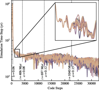
Figure 1: Evolution of the global time-step of the simulation over the course of the simulation (with each line a different clone simulation), demonstrating that even with a fixed random seed the non-deterministic parallelism of SWIFT causes divergences in the time integration as early as a few hundred Myrs into the simulation. Time-steps have been smoothed using a gaussian kernel over the nearest 32 to highlight the long-term trend. Once the time-step has deviated between the simulations, they will draw different random numbers (and there is no reasonable way to keep such number synchronised), leading to uncontrollable deviation in the impacts of star formation and feedback. Timing lines are only representative as they show the current time at that step number for a random clone simulation, apart from the first line at $a=0.06$ which represents the time ($\approx 300$ Myr) at which the first star particle is formed. We additionally note that all of the lines presented here are valid and accurate. Simulations that only consider one realisation of their model would simply choose one of these lines (or another equally valid set of time-steps).

These volumes were evolved to redshift $z=0$, with full particle snapshot dumps at redshifts $z=$ 7, 5, 4, 3, 2, 1.5, 1, 0.75, 0.25, 0.2, 0.1, 0.05, 0.01, 0.001 and $0.0$. These snapshots were then analysed with the VELOCIraptor halo finder (Elahi et al., 2019), producing group catalogues based on the 3D Friends of Friends (FoF) algorithm, that were then further processed using the swiftsimio toolchain (Borrow & Borrisov, 2020; Borrow & Kelly, 2021).

2.5 Impact of Non-Determinism

Many factors can impact the (non-)deterministic nature of a simulation code, some of which are relatively hidden to users. The use of non-blocking and asynchronous communication patterns (as in SWIFT) may lead to different arrival times of data, dependent on network conditions, that could then lead to changes in results. Even synchronous, blocking, communications may have significant non-determinism if they are implemented in a non-deterministic way within the chosen communication library, or the number of communication nodes is changed. In practice a single-threaded code that has an entirely deterministic set of algorithms can have its result depend on infrastructure choices such as the instruction set available on the processor, compiler, or even compilation options. Single Input Multiple Data (SIMD) instruction sets (such as the AVX2 and AVX-512 instruction sets available on our machine) and aggressive compilation options (such as -O3 or -ffast-math), can (for instance) change the order of operations and unroll loops for a performance benefit. These changes lead to different assembler output and hence different round-off errors for the exact same input code, even when using the same compiler, compared to an un-optimised counterpart. As such, we employ the exact same compiled binary in all of our tests (including the dark matter-only simulation, which in SWIFT can be performed without the need to re-compile).

Due to the non-deterministic nature of SWIFT, it was not necessary to change the random seeds in the clone simulations in order to investigate the impact of stochasticity. Fig. 1 shows the variation in the current time step, the time interval over which the active set of particles are being evolved, as a function of the number of steps. After only a few thousand steps (at $z\approx 15$, before significant sub-grid physics effects begin) the evolution of the simulations diverge due to differing round-off errors within the calculation as expected, and due to the feedback from the first stars. This is despite the fact that all time-steps across all clones are discretised in a similar manner, using the typical power-of-two hierarchy (see e.g. Hernquist & Katz, 1989; Borrow et al., 2021).

As the random number generator takes as input the current step, from the point at which the various simulations diverge in their step-simulation time-step curves, each clone will naturally use a distinct sequence of random numbers. This effect can spread throughout the volume due to the time-step limiter employed in the hydrodynamics, which does not allow neighbouring particles time-steps to differ by more than a factor of four (Borrow et al., 2022). We stress here that there is no ‘correct’ series of time-steps that the code should take to evolve to the ‘true’ answer. Each simulation takes a valid path that is dependent on small variations in input properties into the time-step calculation that diverge due to differing round-off errors in the calculation. All simulations follow a similar average path in this figure, with the time step decreasing with the number of steps taken as denser structures build up within the volume.

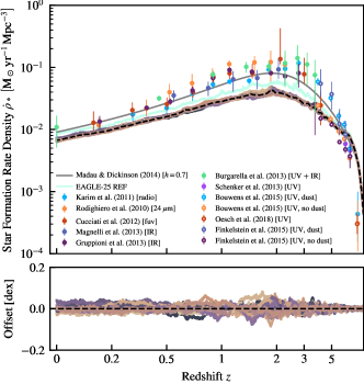
Figure 2: The global (cosmic) star formation rate density history for the various clone simulations (top) and deviations from the median (bottom). Each line shows a different clone, with the black dashed line showing the median across all clones. There is very little (less than 0.1 dex) scatter in this relation across all time, with the variation peaking when the cosmic star formation rate peaks. Data in the background comes from multiple sources, including Madau & Dickinson (2014); Karim et al. (2011); Rodighiero et al. (2010); Cucciati et al. (2012); Magnelli et al. (2013); Gruppioni et al. (2013); Burgarella et al. (2013); Schenker et al. (2013); Bouwens et al. (2015); Oesch et al. (2018); Finkelstein et al. (2015). In addition, we show the same volume (EAGLE 25 REF; aquamarine line) simulated with the original EAGLE code and reference model as in Schaye et al. (2015).

Fig. 2 shows the variation in the global (cosmic) star formation rate density (SFRD) as a function of cosmic redshift, with the same line colours as Fig. 1. We additionally show the median across the clones at each redshift as the black dashed line, and the offset of each clone from this median in the bottom panel. For comparison, we show the original EAGLE Ref model (Schaye et al., 2015; Crain et al., 2015; Furlong et al., 2015) on the same EAGLE-25 volume, at the same resolution, in aquamarine. The systematic offset between our clone simulations and this original EAGLE model (simulated with a modified version of the Gadget code; Springel, 2005) is due to the recalibration of model parameters when moving to SWIFT (see §2.2), as well as the aforementioned model changes. Both simulations undershoot the observational data shown at $z<3$.

Fig. 2 shows that variations between the clone simulations are small and typically less than 0.1 dex. The scatter in the SFRD peaks when the star formation rate peaks, at around $z=2$. The level of scatter in this relation is strongly dependent on the simulation volume size; considering an infinitely large volume, variations between the growth of individual haloes will be washed out in this globally averaged metric.

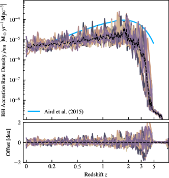
Figure 3: The global black hole accretion rate density (BHARD) history for all clone simulations (top) and variation from the median (bottom). Each line shows a different clone, with the black dashed line showing the running median. There is significant variation between clones, shown in the lower panel, but this is consistent with the high level of variability of the BHARD on short timescales within an individual simulation. In the background, we show observational data from Aird et al. (2015), spanning the range $z=0.0-5.0$.

Fig. 3 shows the variation in the instantaneous global black hole accretion rate density (BHARD) between the clone simulations. The variability in this quantity is significantly higher ($\approx$ 2 dex) than for the global star formation rate density. This can primarily be attributed to two main (connected) reasons: the much poorer sampling of black holes (at $z=0$ there are of order thousands, compared to the millions of star particles that have effectively sampled the SFRD), and the high cadence variability of the BHARD within an individual clone simulation (see also McAlpine et al., 2017; Nobels et al., 2022, for further work on this in the EAGLE model). Even between these 16 clones, we are not able to extract a smooth and stable median BHARD, suggesting an extreme level of variability.

In summary, there is significant variability between the clone simulations, but volume averages can wash this out even in small boxes.

3 Matching Haloes

To investigate how the properties of individual galaxies are affected by random differences between simulations, haloes must be matched between the clones. Matching haloes in a context where the aim is to find differences between each halo that is matched presents a problem; how can we develop a method that allows for robust matching, producing few false positive matches, and allows for potentially substantial differences in the mass content of haloes between clones?

There are a number of strategies for matching haloes between simulations, usually employed to match dark matter only simulations to baryonic counterparts. A common strategy is to use the $n$ most bound particles of each halo, and find the halo in another simulation within which they reside (e.g. Velliscig et al., 2014; Schaller et al., 2015; Bose et al., 2018, 2019; Lovell et al., 2018; Genel et al., 2019). This strategy can have issues when trying to match haloes that are undergoing a merger, which we will see are crucial to understanding the impact of stochasticity. Instead, we employ a strategy that matches haloes by their co-moving final-state position in the volume.

To match haloes between clone simulations, we first match all haloes in each clone with a single, common, dark matter-only ‘parent’ simulation. We choose to do this as stochastic effects in dark matter-only simulations have been shown to be significantly smaller than those in full hydrodynamical simulations (Genel et al., 2019). Then matches in the clone simulations are back-propagated through matches with the same halo in the dark matter-only parent. Matching via a dark matter-only parent also prevents one of the clone simulations being considered the ‘main’ simulation and allows for fair comparisons between all clones. Only central haloes (i.e. not satellites) are matched between simulations, and within the rest of the paper unless explicitly stated all halo properties correspond to those of the central subhalo.

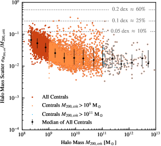
Figure 4: Reduced scatter in halo mass $M_{\rm 200,crit}$, defined as the ratio between half of the 16-84 percentile range of masses ($\sigma_{M_{\rm 200,crit}}$), for three different mass cuts in our matching procedure. Red points show matches for all central haloes, orange for haloes with $M_{\rm 200,crit}>10^{9}$ M_⊙, and blue for haloes $M_{\rm 200,crit}>10^{11}$ M_⊙. Matches show an extremely high level of consistency between these mass cuts. Black points show the median and 16-84 percentile range of halo mass scatters. Horizontal dashed lines show, as a guide, representative scatter as a percentage of the original halo mass and the corresponding log-space (dex) offsets.

Haloes are matched using their comoving positions in the volume. The centres of the haloes in the dark matter only simulation, as defined by their most bound particle, are used to build a KDTree. This tree is then searched using the positions of all haloes in each clone simulation in turn for the nearest 10 haloes. Then, the halo that matches the mass ($M_{\rm 200,crit}$) of the parent halo within 50% and has a distance between the two haloes of less than the $R_{\rm 200,crit}$ of the parent is considered to be the match. For haloes to be included in any analysis they must be matched to at least half of the clone simulations (which in practice removes only a handful of haloes). As we will see later, our strategy naturally leads to no conflicts, but when there are some we choose the halo that is closest in mass. In the following discussion we aim to demonstrate how robust our matching procedure is, though one possible drawback of this method is that it assumes there is a one-to-one matching between central haloes.

Fig. 4 shows how the scatter in halo mass, defined as half of the 16-84^th percentile range of a quantity matched across clones, correlates with the median halo mass matched across clones. Throughout the paper we use this metric, written as

$$\sigma_{x}=\frac{{x}_{{\rm P}_{84}}-{x}_{{\rm P}_{16}}}{2},$$ (5)

where ${x}_{\rm{P}_{y}}$ is the y^th percentile of the distribution of variable $x$, to quantify the scatter between clone simulations. In most cases, we show the reduced quantity (i.e. $\sigma_{x}/x$) where we reduce by the median value matched across clones. We vary the minimal mass at which we match haloes (increasing the distance between haloes), to demonstrate the accuracy of our matching methodology.

At the lowest halo masses, scatter is significant, up to 10% of the total mass of the halo (and more in extreme cases). This is likely due small differences in the coordinates of individual particles that place them just outside of the $R_{\rm 200,crit}$ aperture, as at the lowest mass ($3\times 10^{8}$ M_⊙), only around 30 particles make up the halo. As the halo mass increases, this ‘shot noise’ decreases to a fixed level of around 2%.

The first thing to note from this figure is that there are no points close to the cut-off mass ratio (50%), meaning that there is not a significant set of haloes being rejected from the matching procedure simply because they have a high intrinsic scatter in halo mass between clones (and hence relative to the dark matter only parent).

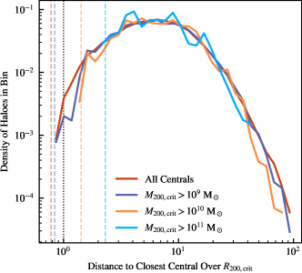
Figure 5: Distribution of distances to the nearest central halo for all halo centres (in units of $R_{\rm 200,crit}$) in the dark matter only simulation above different halo mass thresholds (coloured lines). Dashed vertical lines show for each cut the minimum distance in the entire volume. Even when resolved haloes of any mass are considered (red line), only a fraction of a percentage point of haloes have a separation less than $R_{\rm 200,crit}$. This indicates that if this snapshot was matched with itself a cut at $R/R_{\rm 200,crit}=1$ alone would prevent almost all false positive matches where we incidentally match a halo with one containing different particles. Hence, false positive match detections require significant movement of haloes (i.e. further than $R_{\rm 200,crit}$) between the dark matter only parent and the clone simulations.

The second thing to note is the almost perfect consistency between matching as the mass threshold is increased. Increasing the mass threshold naturally increases the minimum distance between field haloes and reduces the number of false positives. This ensures confidence that our matching procedure is robust, even if the properties of the galaxies resident in these haloes show significant variation in their properties. For all parent haloes the closest separation between field haloes is almost always larger than the match distance criterion (see Fig. 5), even across the mass range.

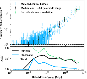
Figure 6: Top panel: the number of substructures for each central as a function of host halo mass. Each blue cross represents the scatter amongst clones (16-84 percentile range), with the cross being centered on the respective medians. The black points and error bars show the median of these medians in 14 equally log-spaced bins, and the length of the bars is the 16-84 percentile scatter of the medians within the bin. The black dashed line shows the extreme $N=1$ case, where the central is the only substructure. The green points show the scaling relation recreated from an individual clone simulation. Bottom panel: the scatter, coloured analogously, from the top panel. The blue line shows the mean (binned) scatter in individual haloes (i.e. the mean length of the blue vertical lines), the green dashed line shows the scatter in the scaling relation as recreated in an individual clone (i.e. the length of the green error bars), and the black line shows the scatter in the medians of the matches (i.e. the length of the black error bars).

Fig. 6 shows the number of resolved substructures within each halo as a function of halo mass. Haloes contain more substructure as the mass increases, as expected (e.g. Kravtsov et al., 2004), though this quantity is clearly resolution-dependent, as substructures can only be tracked down to a minimum of 30 particles, or $M_{\rm 200,crit}\approx 3\times 10^{8}$ M_⊙.

In this case we see both large levels of scatter between clones (i.e. the scatter for a given halo, shown by the blue lines, is large) at low mass, and large intrinsic scatter (i.e. the scatter in the median, shown by the black lines) at high mass. The number of substructures considered bound to a given halo can easily vary by 100% at the low-mass end ($M_{\rm 200,crit}\approx 10^{10}$ M_⊙), with this meaning that the halo has either a single additional substructure or not. This can occur if the merger time is different between clones, or if a very small substructure is just above or below the minimum mass for the halo finder.

At the high-mass end ($M_{\rm 200,crit}\approx 10^{12}$ M_⊙), the scatter in this relation is mainly dominated by differences between the individual haloes’ accretion histories and substructure abundances. The scatter between clones is very small (less than 5%), whereas there can be nearly half a dex of variation within each mass bin. As such, within this regime, we would expect the accretion and merger history of individual bound haloes to be similar between the clone simulations.

4 Galaxy Scaling Relations

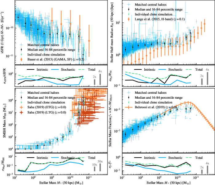
Figure 7: Four key scaling relations, all at $z=0$ and as a function of galaxy stellar mass: specific star formation rate (sSFR; top left, computed from the star particles and averaged over 1 Gyr), galaxy size (stellar half-mass radius within a fixed 50 kpc aperture; top right), black hole mass (most massive black hole; bottom left), and the halo stellar mass fraction ($f_{*}$; bottom right), plotted, for reference, with various observational datasets. Blue crosses show the run-to-run scatter, representing the 16-84 percentile range for each matched halo (crossing at the median across clones). Black points show medians and 16-84 percentile ranges in bins of stellar mass for the medians of the individual halo matches. Green points show the scaling relation binned in a similar fashion, but for only one randomly selected clone. The smaller, lower, panels in each subplot each show three lines representing the scatter in the medians of the matches (i.e. representing the same size as the error bars in the black points, an estimate of the intrinsic scatter) in black; in blue, the median individual scatter in each bin (i.e. the median size of the blue error bars, our estimate for the scatter due to stochastic effects); and as green dashes the total scatter in an individual scaling relation measured from a single clone.

In Fig. 7 four key galaxy scaling relations are shown, with each blue cross representing the 16-84 percentile scatter amongst the clone simulations for matched haloes, with the cross placed at the median point. In black, we show the binned scaling relation (of the medians across clones) and its 16-84 percentile scatter as an indication of intrinsic halo-to-halo scatter when ‘random’ variations are smoothed over. Finally, in the background we show a selection of observational data as a visual reference. As these data are at various redshifts, not matched with the simulations, we show them primarily to demonstrate differences between the scatter in the observed relations relative to the random variability of individual haloes. Each of the properties is shown as a function of galaxy stellar mass, calculated within a fixed 50 kpc aperture.

The smaller panels in Fig. 7 show how the scatter in three cases changes with galaxy stellar mass. In blue, we show the median value (within 14 equally log-spaced bins across the stellar mass range) of the scatter between clone simulations, to demonstrate the typical random variability of galaxies due to stochasticity. This represents half of the median vertical length of the blue crosses in the top panels. In black, we show the scatter in the intrinsic scaling relation, representing the scatter in the average properties (across clones) of the galaxies. This corresponds to half of the length of the vertical black lines in the upper panel. In a green dashed line, we show the scatter of the scaling relation measured in a randomly chosen clone simulation, which arises from both intrinsic and stochastic scatter. This can be thought of as, on average, adding in quadrature the offset from the median line to the center of the thin blue crosses (the median across clones for that object) with a displacement from this median, bounded roughly by the extent of the thin blue lines.

The top left panel of Fig. 7 shows the specific star formation rate (sSFR$=\dot{M}_{*}/M_{*}$) of galaxies against their stellar mass. The star formation rates were recalculated from the birth times of stars in each galaxy to reconstruct a 1 Gyr averaged star formation rate. This was done to smooth over short-timescale fluctuations in the instantaneous star formation rates. 1 Gyr also happens to be of the order of the halo dynamical times, and as such the star formation rate on these timescales should mainly be driven by the accretion history, and should be relatively insulated against small-scale variations that are susceptible to individual round-off differences (Iyer et al., 2020). We compare our sSFR relation against the Bauer et al. (2013) results from the GAMA survey, which only includes galaxies that are considered to be star forming, (sSFR$>10^{-11}$ yr^-1). Here, we include all central galaxies to investigate the quenching behavior at stellar masses $M_{*}>10^{10}$ M_⊙.

The first notable property in the sSFR relation is that when using a standard quenching definition (of sSFR$<10^{-11}$ Gyr^-1) some of the clone galaxies, with fundamentally similar accretion histories (note the typical 2% variation in halo mass from Fig. 4 and less than 5% variation in substructure abundance at high mass in Fig. 6), may be considered quenched and others active.

The vertical scatter in the sSFR of individual galaxies can reach up to 1 dex, though the average scatter of clone galaxies (blue line in the lower panel) is significantly lower than the intrinsic scatter in the scaling relation (black line). Throughout the mass range shown, the scatter in the measured scaling relation in an individual clone is dominated by the intrinsic scatter (black line), except at the lowest masses of $M_{*}<10^{9}$ M_⊙. In this regime, the two components of scatter combine, leading to significantly larger measured scatter than the intrinsic level. The other exception is at the very highest masses, where the stochastic variability rises rapidly due to the onset of variable quenching.

The top right panel shows the stellar mass-size relation, compared against data from the GAMA survey (Lange et al., 2015). Here, we use the projected stellar half-mass size of galaxies measured within a fixed 50 kpc aperture. Sizes of the lowest-mass galaxies ($M_{*}\lessapprox 10^{9}$ M_⊙) are artificially increased in the simulation due to spurious size growth from sampling noise in gravitational interactions between stars and dark matter (Ludlow et al., 2019; Wilkinson et al., 2022). Within this regime we also see increased scatter between the clone galaxies, with the scatter between clones dominating over the intrinsic scatter. It is foreseable that the processes leading to inflated galaxy sizes (spurious gravitational heating, oversoftening of sizes), especially in a regime where there are relatively few ($<1000$) particles resolving each galaxy, could influence the scatter between clones.

There are a number of galaxies significantly above the median, with extremely large (close to 1 dex) scatter in their sizes. These galaxies are typically ongoing mergers, with the central in some cases being identified alone (i.e. post-merger, with all galaxies collected into one central), and in other cases the two merger components being identified separately. We will come back to this point in §5. At the highest masses, we see that the scatter in galaxy size returns to a low level comparable to the scatter in stellar mass, with the overall scatter in each scaling relation corresponding to the intrinsic scatter.

The bottom left panel shows the galaxy stellar mass-black hole mass relation. There is significant scatter in this quantity between the clone simulations for black holes in the rapid growth phase ($10^{6}<M_{\rm BH}/{\rm M}_{\odot}<10^{8}$ and $10^{9}<M_{*}/{\rm M}_{\odot}<10^{11}$ Bower et al., 2017; McAlpine et al., 2018) of up to 1 dex. This does not correspond with significant scatter in stellar mass, though, with the largest scatter in stellar mass appearing at the high-mass end, as confirmed in the bottom right panel showing the stellar to halo mass ratio.

In almost all cases, the scatter in $M_{\rm BH}$ is dominated by the intrinsic scatter in the scaling relation, but this is misleading in the range $10^{10}<M_{*}/{\rm M}_{\odot}<10^{11}$ where the gradient of the scaling relation is large within the single bin leading to a large predicted scaling relation scatter. The average scatter in black hole mass in this regime is approximately equal to the difference between the current and prior median at one dex lower stellar mass. Finally, the average clone-to-clone scatter reduces at the high-mass end rather sharply and shows significantly less variation than the comparison scatter data from Sahu et al. (2019), though measurements of black hole mass are highly uncertain with errors of greater than 1 dex in many cases.

In the bottom right panel, we show the relationship between the stellar mass of galaxies and their halo stellar mass fraction, defined as the ratio between the galaxy stellar mass and $M_{\rm 200,crit}$. We compare against results from the 2019 release of UNIVERSEMACHINE (Behroozi et al., 2019). In almost all cases, aside from the very lowest masses, we see that the scatter in the stellar mass-halo mass relation is dominated by the intrinsic scatter on average. However, we have a number of galaxies that show up to 0.5 dex scatter in stellar mass even at high masses ($M_{*}>10^{10}$ M_⊙), which is in stark contrast to the results from Keller et al. (2019) who showed that scatter in stellar mass should decrease with increasing mass when considering isolated galaxies. The obvious difference here is that we are not considering purely isolated cases, and include AGN feedback. A number of high-scatter cases can originate from ongoing mergers (Davies et al., 2021). In addition to mergers, we see that the average clone-to-clone scatter in stellar mass fraction increases at the very highest masses. It is unlikely that all of these galaxies are currently undergoing a major merger, and we will revisit this point in §6.

Our levels of scatter in stellar mass are roughly comparable to the results presented in Genel et al. (2019), who also employed full cosmological volumes but used a different code and model, though at a similar resolution. Genel et al. (2019) report that their average standard deviation (a measure comparable to our scatter) between clone galaxies is of order 0.1 dex at $z=0$ for stellar mass and stellar half-mass size, though they designed their simulations to include a perturbation at $z=5$, with the difference between clones growing over time, with our clone-to-clone divergence beginning at $z=15$. They additionally see larger scatter in specific star formation rate (also 1 Gyr averaged), typically around 0.2 dex, which is consistent with our results. The similarity between the scatter in both (completely independent) galaxy formation models, implemented in completely different codes, with different parallelisation strategies, is remarkable.

As a general point, if the intrinsic scatter dominates, this leads to similar scatter measured in the scaling relation from a single clone. In cases where the stochastic noise dominates, however, the total scatter is a combination of both the intrinsic and noise scatter.

5 A Case Study

In this section the properties of a halo that has been selected to be “uninteresting” (with typical scatter in stellar mass) are explored to investigate the origins of the scatter between clone simulations.

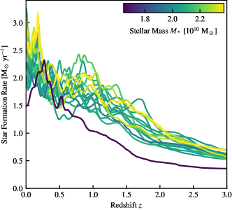
Figure 8: The star formation rate (averaged over the birth times of 256 particles at each point, and smoothed using a Gaussian filter over the nearest 128 points for clarity) recovered from $z=0$ stellar particles, for a single galaxy with $M_{*}\approx 2\times 10^{10}$ M_⊙ matched in each of the clone simulations. Each line is coloured by the $z=0$ stellar mass of the galaxy, which shows a variation of $\sim 10\%$. The outlier shown in dark purple is indeed matched correctly, and will be discussed further in this section.

In Fig. 8 we show the star formation rate of the galaxy in each of the 16 clone simulations from $z=3$ to $z=0$. We recover the star formation rate from the birth times of the star particles belonging to the galaxy at $z=0$, calculating a moving average based upon the birth times of 256 particles to ensure each point is captured with the same Poisson error.

There is $\approx 0.1$ dex scatter in the final-state stellar mass (of $\approx 2\times 10^{10}$ M_⊙) that is created through the varying star formation rate across cosmic time. The majority of the curves overlap significantly, with $\approx 30\%$ variation in star formation rate at any given time. It is notable that the highest mass galaxy (yellow line) does not have a continuously higher star formation rate across time, but it has an above-average star formation rate for the longest.

There is, however, an outlier (dark blue curve) that has a significantly lower star formation rate (by about 25%) across much of the history of the galaxy, corresponding to a lower final stellar mass. Additionally, it lacks the peaks between $z=2$ and $z=0$ shown in the other curves, suggesting a suppressed merger history, which we will discuss in detail in the following text.

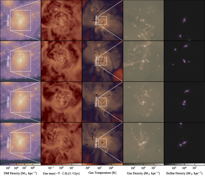
Figure 9: Various properties of the case study halo at $z=0$. From left to right, we show the projected dark matter surface density (projection depth 500 kpc), the convergent gas velocity divergence (a tracer of shocks, projection depth 100 kpc), the mass-weighted gas temperature (100 kpc), the gas surface density (100 kpc), and finally the stellar surface density (100 kpc), zooming in from left to right. In the stellar density image, particles associated with the matched central halo are highlighted in pink, whilst particles not associated with the central halo are white. Clone haloes are ordered from lowest to highest mass from top to bottom.

In Fig. 9 we display maps of different properties of four clones of this galaxy as projections through the volume (projection depths are indicated in the caption). From top to bottom we show a selection of the lowest to highest mass clone galaxies whose star formation rates we shown in Fig. 8. Horizontally, the panels show the dark matter projected density along the line of sight, the convergent gas velocity dispersion (which highlights shocks), the projected gas temperature, and finally the projected gas and stellar densities.

First, the dark matter density image (shown with a side length of 2 Mpc) demonstrates that there may be different positions of substructures between clones. In Genel et al. (2019), it is shown that there is on average a difference of $\approx 2$ kpc between dark matter particles at $z=0$ between clone simulations, indicating that there is a significant impact on small-scale dynamics that bleeds through to infall times of substructures as seen here (e.g. the placement of the two substructures just inside the inset square at 11 and 12 o’clock).

Zooming in to a 1 Mpc box side length (second column), we now turn to look at the large scale gas dynamics. The value of $\max(-\dot{\nabla}\cdot\vec{v}_{\rm g},0)$ is shown projected along the line of sight to highlight shocks within the circumgalactic medium (CGM) and intergalactic medium (IGM) around this galaxy. Though the general picture is similar in all four cases, there are significant differences in the specific placement of shocks, indicating differences in the large-scale gas dynamics and feedback timing between clones (e.g. the bubble at 2 o’clock in the third row).

On the same scale we show the projected gas temperature along the line of sight (third column), further indicating significant differences between the gas dynamics in the CGM and IGM. Though the size of the hot gas halo surrounding the galaxy is well constrained across clones, the detailed structure, including the direction of outflows, and the abundance and placement of cold gas clumps, shows differences. In the top row, there is a substructure undergoing stripping of its cold gas (9-12 o’clock, just outside the 200 kpc inset box), leaving a trail within the CGM. The trail is completely absent in the other panels, as the gas has broken up into hotter and more diffuse clumps.

The two rightmost columns show zoom ins of the structure of the galaxy disks themselves, with an image of side length of 200 kpc. Here we begin to see large differences in the merger timing between the clones, illuminating why the star formation rates of the galaxies are so different in Fig. 8. This final-state galaxy is an ongoing merger between three individual bound objects at $z=0$. Not only are the galaxies in the top row (lowest mass) smaller in size, they have proceeded less than their clones into the merger process, with one of the three infalling galaxies (bottom right, edge of the panel) not being included in the bound structure and hence not being included as part of the star formation rate calculation (stars that are included as ‘bound’ to the central are highlighted in pink in the right column, with this being essentially all of them except the incoming galaxy that is mostly hidden in the top row, and the small dwarf at 8 o’clock in the second row).

The ISM and CGM around these galaxies show significant differences between clones. The morphology of dense inflows seems to be completely unconstrained between clones, with the number of dense, dark (i.e. not containing stars), substructures showing significant variation. In the second row, there are two additional luminous satellites (see stellar image) close to the merging galaxies that have no analogues in the other clones.

Such large variation in morphology between clones presents potential issues for studies of the halo-galaxy connection in cosmological simulations of small numbers of objects. On the largest scales, there are relatively minor differences between the haloes of these galaxies, with some substructure being moved around. On the galactic scale, however, even if stellar masses are similar, the CGM and specific merger timing of the galaxies remains unconstrained.

We stress here that all of the galaxies predicted in different clones are equally ‘accurate’. Although they all have slightly different feedback onset, merger, and growth timescales, they are all valid predictions of the galaxy formation model for such a history. These galaxies all live in extremely similar large-scale environments, and in all cases constitute a $z=0$ system that is either a pre-triple merger or an ongoing triple merger. As shown in Fig. 7, the overall properties of galaxies are well constrained between clones, further illustrated here with the similar stellar masses. Tying the properties of the local CGM around such systems to the properties of the environment or galaxy, however, requires investigation of many haloes, or resimulation of the same galaxy (cloning, as here), to understand the impact of stochastic variations on the results of the study.

Finally, we note that even though we attempted to match all 16 clones, only 14 matches were successful with our strategy. This was also the case with a traditional particle matching method, and demonstrates the limitations of a one-to-one matching strategy. As shown here, the most extreme cases are those that are the furthest pre-merger, and in the unmatched two cases, the three major galaxies represented here are entirely pre-merger, whereas in the dark matter-only case the halo is entirely post-merger. To match this scenario, we would need to devise a strategy to perform three-to-one matching, which was not anticipated before the onset of this work.

6 Galaxy Property Scatter

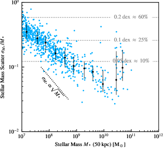
Figure 10: Scatter (using the same definition as Fig. 4) in the galaxy stellar mass measured in a 3D 50 kpc aperture for all matched galaxies (blue points). Black points show median scatter in bins of $M_{*}$, with the error bars representing the 16-84 percentile range. The black dotted line shows the expected scaling (with the normalisation moved) if the scatter represented Poisson noise sampling for the stellar particles. The expected normalisation in this case would be approximately 0.1 dex at $M_{*}\approx 10^{7.5}$ M_⊙ with the line moved for clarity.

One of the most fundamental galaxy properties, used widely within carefully designed scaling relations, is the galaxy stellar mass. Simulation suites are now often explicitly tuned to reproduce the stellar mass of galaxies (either through the stellar mass function alone, like EAGLE; Crain et al. 2015, or additionally through the stellar mass-halo mass relation, like Illustris-TNG; Pillepich et al. 2018). It is hence imperative that galaxy formation simulations are able to reliably produce representative stellar masses, relative to their input physics and parameters.

Fig. 10 shows the scatter in galaxy stellar masses, using 50 kpc 3D fixed stellar apertures following de Graaff et al. (2022). The scatter in stellar mass is calculated as for halo mass in Fig. 4, representing half of the 16-84 percentile range across all clone simulations within which each halo was matched.

In simulations of isolated galaxies, Keller et al. (2019) showed that the scatter in stellar mass scaled as a Poisson-like error, with $\sigma_{M_{*}}\propto\sqrt{M_{*}}$. For low-mass galaxies ($M_{*}<10^{10}$ M_⊙), we find that this is broadly true in the cosmological clones too, although the scatter scales with stellar mass as approximately $\sigma_{M_{*}}\propto M_{*}^{-2/3}$. This additional scatter in more realistic cosmological simulations is anticipated, as Keller et al. (2019) found that scatter in stellar mass was significantly increased during merger events which occur naturally in a cosmological environment.

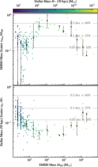
Figure 11: Scatter in SMBH mass (top) and stellar mass (bottom) as a function of SMBH mass. Points show individual matched galaxies, coloured by stellar mass, with black points and error bars showing the median and the 16-84th percentile range. As black holes grow, their masses stabilise across clones simulations, but the associated highly energetic and stochastic AGN feedback leads to progressively larger scatter in the stellar mass of the host galaxies.

The more surprising feature in Fig. 10 is the presence of an up-tick in scatter at galaxy masses of $M_{*}\gtrapprox 10^{10}$, where feedback from active galactic nuclei (AGN) becomes significant (Bower et al., 2017; Bahé et al., 2022). To investigate the impact of black hole growth (and its associated feedback) on galaxies, Fig. 11 shows the scatter associated with supermassive black holes (SMBHs). These are identified as the most massive black hole resident in the host galaxy, and are typically placed at the centre of the haloes, where they provide most of the AGN feedback, through the recentering prescription (see Bahé et al., 2022).

We first focus on the bottom panel, which shows the scatter in stellar mass (the same as Fig. 10), but now as a function of black hole sub-grid mass. At low black hole masses, we see relatively high scatter in stellar masses due to these systems having a correspondingly low stellar mass and hence high Poisson-like scatter (see above). As the black hole mass grows beyond $M_{\rm BH}>10^{6}$ M_⊙, the scatter in stellar mass begins to level off and increase again at $M_{\rm BH}>10^{7}$ M_⊙.

In our model, black holes are seeded at $10^{4}$ M_⊙, and grow through Bondi-Hoyle accretion of ambient gas. In the top panel of Fig. 11, the scatter in black hole masses is shown, with high levels of black hole scatter up to 100% being sustained for black hole masses $10^{6}<M_{\rm BH}/{\rm M}_{\odot}<10^{8}$ where these objects undergo rapid growth relative to their host galaxy (see the stellar mass-black hole mass relation in Fig. 7). As the onset of this rapid growth has a random component (i.e. when the first dense gas settles within the accretion radius), the timing of the growth phase is uncertain and hence quickly leads to large variation in the black hole masses. In these cases, the black hole mass is determined by relatively few accretion events, and as such each accretion event comes along with significant black hole growth, making the timing (which is stochastic) crucial.

Genel et al. (2019) did not report an increase in stellar mass scatter at the highest masses, although they found the same reduction in black hole mass scatter at high masses that we report. This may be due to the different AGN feedback implementations used in the two codes. For instance, the Illustris-TNG model used by Genel et al. (2019) uses a kinetic radio mode, which may have a different level of susceptibility to small timescale variations in gas availability.

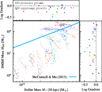
Figure 12: Zoomed-in region of the stellar mass-black hole mass relation (Fig. 7). Individual colours now show single haloes matched between the clone simulations, with the dotted line showing a linear fit to the data (in log space). The panels to the top and right show, for each axis, the gradient of this fit as a function of stellar mass and black hole mass respectively. The grey dashed line in these two panels shows a gradient of zero, i.e. there is no dependence of the black hole mass on stellar mass (or vice-versa). Points lying above or right of the line indicate that the black hole mass grows as the stellar mass grows, whereas points that lie below the line indicate that the stellar mass in the halo is lower the higher the black hole mass is.

Fig. 12 shows the correlation between the scatter between stellar mass and black hole mass between clones for individual haloes. Each colour shows a single halo, in all clone simulations, and its scatter in this space. To guide the eye, we fit straight lines to the scatter from each halo, and show their gradients on the adjacent panels as a function of the two variables. In the background we show the McConnell & Ma (2013) data to show the regime where galaxies are believed to self-regulate due to AGN feedback, with us plotting their bulge mass data as a proxy of galaxy stellar mass meaning there is an expected horizontal offset.

Across the mass range shown, black holes suppress the growth of galaxies. There is an anti-correlation between $M_{\rm BH}$ and $M_{*}$ within clones of individual galaxies. This leads to a negative gradient in $M_{\rm BH}/M_{*}$, as indicated by the top and right panels of Fig. 11.

This figure begins to enlighten us on the trends that were observed in Fig. 11, with galaxies at $M_{*}<3\times 10^{10}$ M_⊙ showing significantly larger scatter in black hole mass amongst clones than their higher mass counterparts, while more massive galaxies show instead an increased diversity in their stellar mass across clones.

Between a black hole mass of $8\times 10^{6}<M_{\rm BH}/{\rm M}_{\odot}<8\times 10^{7}$, the gradient of $M_{\rm BH}/M_{*}$ indicates that the black holes are strongly suppressing growth, as amongst clones lower black hole masses correspond to more massive galaxies. In these scenarios, we would expect the accretion history of the galaxies to be similar, but differences in initial accretion (and hence feedback) timing lead to different output stellar masses due to the changing onset times of quenching.

At the highest black hole masses, with $M_{\rm BH}>10^{8}$ M_⊙, the anti-correlation between black hole mass and galaxy mass weakens, with the gradient of the $M_{\rm BH}/M_{*}$ relationship returning to $\approx 0$.

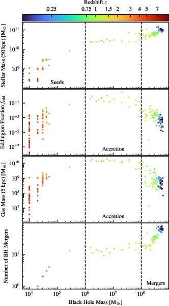
Figure 13: Tracks of a single clone galaxy (the most massive in the simulation volume), in four different key metrics. Each colour represents a different snapshot in time, with each point representing one clone of this galaxy. From top to bottom we show the stellar mass of the host galaxy, the Eddington fraction of the accreting black hole (at $f_{\rm Edd}=1$, the black hole is maximally accreting), the gas mass within a fixed 5 kpc aperture around the black hole, and the total number of mergers experienced by the black hole. Two vertical dashed lines separate the three growth phases of the black hole, from it being a seed black hole, to it accreting close to its maximum rate, to finally merger-driven growth at masses $M_{\rm BH}>10^{8}$ M_⊙.

To investigate the relationship between the accretion onto black holes, the galaxy they live in, and black hole growth, we now turn to tracking an individual galaxy across both time and clones. In Fig. 13, we show the history of the most massive galaxy in the volume, with a $z=0$ stellar mass of $M_{*}\approx 10^{11}$ M_⊙. Each colour shows a single point in time, with each point of a given colour showing the relationship between the property and black hole mass in a given clone. We split the panels horizontally into three segments, depending on the typical stage of black hole growth.

At masses $M_{\rm BH}<10^{6}$ M_⊙, black holes are still effectively seeds; they have not yet accreted the equivalent of one gas particle. The black holes are accreting at significantly below the Eddington rate, with $f_{\rm Edd}\lesssim 10^{-3}$, due to both the low black hole mass (Bondi accretion scales as $\dot{M}_{\rm BH}\propto M_{\rm BH}^{2}$) and low surrounding gas density for accretion, and indicating extremely long growth timescales through accretion. Typically scatter in the black hole mass (i.e. horizontal scatter for a given time) is driven by mergers with other seeds. Note how the scatter across black hole mass is quantised at values of $M_{\rm BH}=\{1,2,3\}M_{\rm BH,seed}=10^{4}$ M_⊙ (see also the number of mergers in the lower panel).

After roughly 10-20 mergers, the black holes have a high enough mass to accrete efficiently from their surroundings. In addition, by this time, the gas density has grown significantly, with in many cases there being $M_{\rm g}>10^{10}$ M_⊙ within 5 kpc of the black hole (see Bower et al., 2017). In this rapid accretion phase ($f_{\rm Edd}\approx 1$), the black holes show significant spread in mass (between $10^{6}<M_{\rm BH}/{\rm M}_{\odot}<10^{8}$), that is roughly independent of galaxy stellar mass. At such high Eddington ratios, the black holes can double their mass in less than 100 Myr, making the onset of such rapid accretion a key determinant in their mass at a given point in time.

After the rapid accretion phase, gas expulsion from the galaxy core leads to quenching of the galaxy, and shuts down black hole accretion (the rapid decline in gas mass with black hole mass, green points). Once this happens, feedback regulates the stellar masses of galaxies (see Booth & Schaye, 2009), with there being a negative correlation between galaxy mass and black hole mass that persists to $z=0$. The increased scatter in stellar mass at the high mass end of Fig. 10 can therefore be understood in terms of the stronger variation of AGN feedback. From this point onwards, the Eddington fraction of the black holes is reduced to less than $f_{\rm Edd}\approx 10^{-3}$, with black holes undergoing many more mergers, indicating that they grow much more slowly. As shown in Bahé et al. (2022), these mergers are mainly with seed-mass black holes, and do not significantly contribute to the mass of the central SMBH.

This case study also highlights how studies on the stochasticity of the model can help us gain insight into the inner workings of the model due to the small changes in accretion history and merger timings they create.

7 Conclusions

Cosmological galaxy formation simulations employ a suite of stochastic sub-grid models to coarse-grain continuous physical processes. These stochastic models enable physics that usually acts on small timescales, and on small masses (relative to the time-step and particle mass resolution in the simulation) to be approximated in an effort to make simulations computationally feasible. In this paper, we have closely examined the impact of these stochastic models on both the resultant global predictions and properties of individual galaxies simulated with the SWIFT code and SWIFT-EAGLE model through 16 re-simulations of the same $25^{3}$ Mpc³ volume labeled as ‘clones’. Our main findings are as follows:

• In Fig. 1, we showed that modern, non-deterministic, task-based codes inevitably lead to deviations between simulations after roughly 1000 steps, or 300 Myr into the simulation, for a 25 Mpc volume. All of these re-simulations are equally valid (or invalid): these deviations arise from round-off errors that accumulate in both the gravity and hydrodynamics calculations, leading to differences in the timings of the first stars and hence first feedback events.

• In Figs. 2 and 3, we showed how even globally averaged properties in a full cosmological volume differ between clone simulations. At a fixed redshift, the star formation rate density is only constrained to $\approx 0.1$ dex, and the black hole accretion rate density only to within $\approx 1.0$ dex, in a 25 Mpc volume. In larger simulation volumes these differences in globally averaged quantities between clones are expected to diminish even further.

• In Fig. 6, we showed that the number of substructures within individually matched FoF haloes is well constrained between clone simulations, especially at masses $M_{\rm 200,crit}>10^{11}$ M_⊙, with the scatter between clone galaxies reducing as mass increases. This metric is likely to be significantly affected by the resolution of our simulations, but it confirms that the accretion history for the most massive haloes is well constrained between clone simulations.

• In Fig. 7, we investigated the impact of differences between clone simulations on our ability to predict scatter in scaling relations with simulations. In some cases, the scatter in scaling relations can be significantly affected by the variability in the properties of individual galaxies. This typically occurs at the lowest galaxy masses, with the clone-to-clone scatter dominating at at $M_{*}\lessapprox 10^{8.5}$ M_⊙, but high levels of variability can occur at high masses where galaxies are well resolved when the property is time-sensitive (e.g. sSFR and galaxy quenching).

• In Figs. 8 and 9, we presented a case study of one individual galaxy across the clone simulations with $M_{*}\approx 2\times 10^{10}$ M_⊙ to investigate the origin of scatter in its properties. Although global properties, such as halo and stellar mass, are well constrained (showing around 10% variation), detailed properties such as the positions of substructure, phase structure of the ISM, CGM, and even IGM were different between clones. Investigations into the halo-galaxy connection, particularly those employing such phase information, must use adequate sampling to suppress the random variability within the galaxy formation model.

• In Fig. 12 we investigated the correlation between scatter in galaxy stellar mass and black hole mass to identify the cause of an increase in clone-to-clone stellar mass scatter at $M_{*}\approx 3\times 10^{10}$ M_⊙. There is a strong anti-correlation between black hole and stellar mass of individual galaxies across clone simulations in the mass range $10^{6}<M_{\rm BH}/{\rm M}_{\odot}<10^{8}$, which weakens at higher black hole masses.

In summary, we have found that whilst the properties of individual galaxies can be significantly impacted by random variations between clones, and hence the stochasticity of modern galaxy formation models, large-scale properties such as galaxy scaling relations are relatively robust against this random variability. The medians of these scaling relations are well constrained, but there is a significant component of the scatter, especially in the poorly-resolved (low-mass) regime, that originates from differences due to random variability. At higher masses, galaxy mergers and those with recent strong feedback events can see huge variation in their measured properties between clone simulations.

It is likely that the differences between clones are driven by the choice to discretise sub-grid models stochastically. Although there may be some component of the scatter that would still remain if all models were continuous (mainly driven by round-off errors causing different timing for e.g. AGN feedback), the residual differences would likely be small, as shown in the appendix of Genel et al. (2019). Despite the additional variability created in the final galaxy properties by these models, they remain extremely useful due to their small memory footprint and their immunity to spurious gravitational heating effects (Ludlow et al., 2021).

These results indicate that analysts of individual objects must be cautious about the unpredictability of galaxy properties due to random variations, notably in certain setups when model parameters are changed, or in constrained realisation simulations aiming to reproduce properties of a given observable object.

Future work should investigate the impact of random variability on satellite galaxies, as well as reconsider the one-to-one matching paradigm that we have explored here; in many cases, the most impacted objects are those that are split into many (generally pre-merger) within clones. It should also consider additional sources of stochasticity (those not based upon random numbers) that were unexplored here, such as stochastic gravitational scattering and the influence of high mass ratios between baryonic and dark matter resolution elements.

8 Acknowledgements

JB and the authors gratefully acknowledge the significant contribution to this paper that Richard G. Bower made. He provided mentorship and advice on this and many other related works, but was unable to take part in the final stages of preparation for this work due to illness. This paper would not have been possible without his expert guidance and support.

The authors thank the anonymous referee for their helpful comments. The authors acknowledge helpful conversations with Ben Keller. YMB gratefully acknowledges funding from the Netherlands Organization for Scientific Research (NWO) through Veni grant number 639.041.751 and financial support from the Swiss National Science Foundation (SNSF) under funding reference 200021_213076. ADL acknowledges financial support from the Australian Research Council through their Future Fellowship scheme (project number FT160100250). EA acknowledges the STFC studentship grant ST/T506291/1. This work used the DiRAC@Durham facility managed by the Institute for Computational Cosmology on behalf of the STFC DiRAC HPC Facility (www.dirac.ac.uk). The equipment was funded by BEIS capital funding via STFC capital grants ST/K00042X/1, ST/P002293/1, ST/R002371/1 and ST/S002502/1, Durham University and STFC operations grant ST/R000832/1. DiRAC is part of the National e-Infrastructure.

8.1 Software Citations

This paper made use of the following software packages:

• Swift: (Schaller et al., 2018)

• VELOCIraptor: (Elahi et al., 2019)

• Matplotlib: Hunter (2007)

• SciPy: Virtanen et al. (2020)

• NumPy: Harris et al. (2020)

• unyt: Goldbaum et al. (2018)

• SwiftSimIO: Borrow & Borrisov (2020); Borrow & Kelly (2021)

Data Availability

All data generated and used in this article were generated using the open source simulation code SWIFT, and use the publicly available VELOCIraptor code for structure finding. The SWIFT-EAGLE model is freely available in the SWIFT repository, as are the initial conditions. All data analysis and reductions were performed with swiftsimio and related open source tools. The data volume of the simulations is large ($\sim 3$ TB), but the underlying computing time to perform them is modest (less than 100’000 CPU hours).

References

- Aird et al. (2015) Aird J., Coil A. L., Georgakakis A., Nandra K., Barro G., Pérez-González P. G., 2015, MNRAS, 451, 1892
- Anglés-Alcázar et al. (2017) Anglés-Alcázar D., Davé R., Faucher-Giguère C.-A., Özel F., Hopkins P. F., 2017, MNRAS, 464, 2840
- Bahé et al. (2022) Bahé Y. M., et al., 2022, MNRAS, 516, 167
- Bauer et al. (2013) Bauer A. E., et al., 2013, MNRAS, 434, 209
- Behroozi et al. (2019) Behroozi P., Wechsler R. H., Hearin A. P., Conroy C., 2019, MNRAS, 488, 3143
- Bondi (1952) Bondi H., 1952, MNRAS, 112, 195
- Booth & Schaye (2009) Booth C. M., Schaye J., 2009, MNRAS, 398, 53
- Borrow & Borrisov (2020) Borrow J., Borrisov A., 2020, The Journal of Open Source Software, 5, 2430
- Borrow & Kelly (2021) Borrow J., Kelly A. J., 2021, arXiv e-prints, p. arXiv:2106.05281
- Borrow et al. (2018) Borrow J., Bower R. G., Draper P. W., Gonnet P., Schaller M., 2018, arXiv e-prints, p. arXiv:1807.01341
- Borrow et al. (2021) Borrow J., Schaller M., Bower R. G., 2021, MNRAS, 505, 2316
- Borrow et al. (2022) Borrow J., Schaller M., Bower R. G., Schaye J., 2022, MNRAS, 511, 2367
- Bose et al. (2018) Bose S., Deason A. J., Frenk C. S., 2018, ApJ, 863, 123
- Bose et al. (2019) Bose S., Eisenstein D. J., Hernquist L., Pillepich A., Nelson D., Marinacci F., Springel V., Vogelsberger M., 2019, MNRAS, 490, 5693
- Bouwens et al. (2015) Bouwens R. J., et al., 2015, ApJ, 803, 34
- Bower et al. (2017) Bower R. G., Schaye J., Frenk C. S., Theuns T., Schaller M., Crain R. A., McAlpine S., 2017, MNRAS, 465, 32
- Burgarella et al. (2013) Burgarella D., et al., 2013, A&A, 554, A70
- Chabrier (2003) Chabrier G., 2003, PASP, 115, 763
- Chaikin et al. (2022) Chaikin E., Schaye J., Schaller M., Bahé Y. M., Nobels F. S. J., Ploeckinger S., 2022, MNRAS, 514, 249
- Crain et al. (2015) Crain R. A., et al., 2015, MNRAS, 450, 1937
- Cucciati et al. (2012) Cucciati O., et al., 2012, A&A, 539, A31
- Dalla Vecchia & Schaye (2012) Dalla Vecchia C., Schaye J., 2012, MNRAS, 426, 140
- Davé et al. (2019) Davé R., Anglés-Alcázar D., Narayanan D., Li Q., Rafieferantsoa M. H., Appleby S., 2019, MNRAS, 486, 2827
- Davies et al. (2021) Davies J. J., Crain R. A., Pontzen A., 2021, MNRAS, 501, 236
- Davies et al. (2022) Davies J. J., Pontzen A., Crain R. A., 2022, MNRAS,
- Dehnen (2014) Dehnen W., 2014, Computational Astrophysics and Cosmology, 1, 1
- Dubois et al. (2014) Dubois Y., et al., 2014, MNRAS, 444, 1453
- Elahi et al. (2019) Elahi P. J., Cañas R., Poulton R. J. J., Tobar R. J., Willis J. S., Lagos C. d. P., Power C., Robotham A. S. G., 2019, Publ. Astron. Soc. Australia, 36, e021
- Faucher-Giguère (2020) Faucher-Giguère C.-A., 2020, MNRAS, 493, 1614
- Feldmann et al. (2022) Feldmann R., et al., 2022, arXiv e-prints, p. arXiv:2205.15325
- Ferland et al. (2017) Ferland G. J., et al., 2017, Rev. Mex. Astron. Astrofis., 53, 385
- Finkelstein et al. (2015) Finkelstein S. L., et al., 2015, ApJ, 810, 71
- Furlong et al. (2015) Furlong M., et al., 2015, MNRAS, 450, 4486
- Genel et al. (2019) Genel S., et al., 2019, ApJ, 871, 21
- Goldbaum et al. (2018) Goldbaum N. J., ZuHone J. A., Turk M. J., Kowalik K., Rosen A. L., 2018, The Journal of Open Source Software, 3, 809
- de Graaff et al. (2022) de Graaff A., Trayford J., Franx M., Schaller M., Schaye J., van der Wel A., 2022, MNRAS, 511, 2544
- Greengard & Rokhlin (1987) Greengard L., Rokhlin V., 1987, Journal of Computational Physics, 73, 325
- Grudić et al. (2021) Grudić M. Y., Guszejnov D., Hopkins P. F., Offner S. S. R., Faucher-Giguère C.-A., 2021, MNRAS, 506, 2199
- Gruppioni et al. (2013) Gruppioni C., et al., 2013, MNRAS, 432, 23
- Harris et al. (2020) Harris C. R., et al., 2020, Nature, 585, 357
- Hernquist & Katz (1989) Hernquist L., Katz N., 1989, ApJS, 70, 419
- Hunter (2007) Hunter J. D., 2007, Computing in Science and Engineering, 9, 90
- Iyer et al. (2020) Iyer K. G., et al., 2020, MNRAS, 498, 430
- Karim et al. (2011) Karim A., et al., 2011, ApJ, 730, 61
- Keller et al. (2014) Keller B. W., Wadsley J., Benincasa S. M., Couchman H. M. P., 2014, MNRAS, 442, 3013
- Keller et al. (2019) Keller B. W., Wadsley J. W., Wang L., Kruijssen J. M. D., 2019, MNRAS, 482, 2244
- Kravtsov et al. (2004) Kravtsov A. V., Berlind A. A., Wechsler R. H., Klypin A. A., Gottlöber S., Allgood B., Primack J. R., 2004, ApJ, 609, 35
- Kugel & Borrow (2022) Kugel R., Borrow J., 2022, The Journal of Open Source Software, 7, 4240
- Lange et al. (2015) Lange R., et al., 2015, MNRAS, 447, 2603
- Lovell et al. (2018) Lovell M. R., et al., 2018, MNRAS, 481, 1950
- Ludlow et al. (2019) Ludlow A. D., Schaye J., Schaller M., Richings J., 2019, MNRAS, 488, L123
- Ludlow et al. (2020) Ludlow A. D., Schaye J., Schaller M., Bower R., 2020, MNRAS, 493, 2926
- Ludlow et al. (2021) Ludlow A. D., Fall S. M., Schaye J., Obreschkow D., 2021, MNRAS, 508, 5114
- Madau & Dickinson (2014) Madau P., Dickinson M., 2014, ARA&A, 52, 415
- Magnelli et al. (2013) Magnelli B., et al., 2013, A&A, 553, A132
- Matthee et al. (2017) Matthee J., Schaye J., Crain R. A., Schaller M., Bower R., Theuns T., 2017, MNRAS, 465, 2381
- McAlpine et al. (2017) McAlpine S., Bower R. G., Harrison C. M., Crain R. A., Schaller M., Schaye J., Theuns T., 2017, MNRAS, 468, 3395
- McAlpine et al. (2018) McAlpine S., Bower R. G., Rosario D. J., Crain R. A., Schaye J., Theuns T., 2018, MNRAS, 481, 3118
- McConnell & Ma (2013) McConnell N. J., Ma C.-P., 2013, ApJ, 764, 184
- Nobels et al. (2022) Nobels F. S. J., Schaye J., Schaller M., Bahé Y. M., Chaikin E., 2022, MNRAS, 515, 4838
- Oesch et al. (2018) Oesch P. A., Bouwens R. J., Illingworth G. D., Labbé I., Stefanon M., 2018, ApJ, 855, 105
- Pillepich et al. (2018) Pillepich A., et al., 2018, MNRAS, 473, 4077
- Planck Collaboration et al. (2014) Planck Collaboration et al., 2014, A&A, 571, A16
- Planck Collaboration et al. (2020) Planck Collaboration et al., 2020, A&A, 641, A6
- Ploeckinger & Schaye (2020) Ploeckinger S., Schaye J., 2020, MNRAS, 497, 4857
- Richings et al. (2014) Richings A. J., Schaye J., Oppenheimer B. D., 2014, MNRAS, 440, 3349
- Rodighiero et al. (2010) Rodighiero G., et al., 2010, A&A, 518, L25
- Rosas-Guevara et al. (2015) Rosas-Guevara Y. M., et al., 2015, MNRAS, 454, 1038
- Roth et al. (2016) Roth N., Pontzen A., Peiris H. V., 2016, MNRAS, 455, 974
- Sahu et al. (2019) Sahu N., Graham A. W., Davis B. L., 2019, ApJ, 876, 155
- Sawala et al. (2013) Sawala T., Frenk C. S., Crain R. A., Jenkins A., Schaye J., Theuns T., Zavala J., 2013, MNRAS, 431, 1366
- Schaller et al. (2015) Schaller M., et al., 2015, MNRAS, 451, 1247
- Schaller et al. (2016) Schaller M., Gonnet P., Chalk A. B. G., Draper P. W., 2016, arXiv e-prints, p. arXiv:1606.02738
- Schaller et al. (2018) Schaller M., Gonnet P., Draper P. W., Chalk A. B. G., Bower R. G., Willis J., Hausammann L., 2018, SWIFT: SPH With Inter-dependent Fine-grained Tasking, Astrophysics Source Code Library, record ascl:1805.020 (ascl:1805.020)
- Schaller et al. (2023) Schaller M., et al., 2023, arXiv e-prints, p. arXiv:2305.13380
- Schaye (2004) Schaye J., 2004, ApJ, 609, 667
- Schaye & Dalla Vecchia (2008) Schaye J., Dalla Vecchia C., 2008, MNRAS, 383, 1210
- Schaye et al. (2015) Schaye J., et al., 2015, MNRAS, 446, 521
- Schenker et al. (2013) Schenker M. A., et al., 2013, ApJ, 768, 196
- Schmidt (1959) Schmidt M., 1959, ApJ, 129, 243
- Smith et al. (2017) Smith B. D., et al., 2017, MNRAS, 466, 2217
- Springel (2005) Springel V., 2005, MNRAS, 364, 1105
- Springel & Hernquist (2003) Springel V., Hernquist L., 2003, MNRAS, 339, 289
- Springel et al. (2005) Springel V., et al., 2005, Nature, 435, 629
- Stinson et al. (2006) Stinson G., Seth A., Katz N., Wadsley J., Governato F., Quinn T., 2006, MNRAS, 373, 1074
- Tremmel et al. (2017) Tremmel M., Karcher M., Governato F., Volonteri M., Quinn T. R., Pontzen A., Anderson L., Bellovary J., 2017, MNRAS, 470, 1121
- Velliscig et al. (2014) Velliscig M., van Daalen M. P., Schaye J., McCarthy I. G., Cacciato M., Le Brun A. M. C., Dalla Vecchia C., 2014, MNRAS, 442, 2641
- Virtanen et al. (2020) Virtanen P., et al., 2020, Nature Methods, 17, 261
- Vogelsberger et al. (2014) Vogelsberger M., et al., 2014, MNRAS, 444, 1518
- Vogelsberger et al. (2020) Vogelsberger M., Marinacci F., Torrey P., Puchwein E., 2020, Nature Reviews Physics, 2, 42
- Weinberger et al. (2017) Weinberger R., et al., 2017, MNRAS, 465, 3291
- Wiersma et al. (2009a) Wiersma R. P. C., Schaye J., Smith B. D., 2009a, MNRAS, 393, 99
- Wiersma et al. (2009b) Wiersma R. P. C., Schaye J., Theuns T., Dalla Vecchia C., Tornatore L., 2009b, MNRAS, 399, 574
- Wilkinson et al. (2022) Wilkinson M. J., Ludlow A. D., Lagos C. d. P., Fall S. M., Schaye J., Obreschkow D., 2022, arXiv e-prints, p. arXiv:2208.07623
- Willis et al. (2020) Willis J. S., Schaller M., Gonnet P., Helly J. C., 2020, arXiv e-prints, p. arXiv:2003.11468