Model free variable importance for high dimensional data

Abstract

A model-agnostic variable importance method can be used with arbitrary prediction functions. Here we present some model-free methods that do not require access to the prediction function. This is useful when that function is proprietary and not available, or just extremely expensive. It is also useful when studying residuals from a model. The cohort Shapley (CS) method is model-free but has exponential cost in the dimension of the input space. A supervised on-manifold Shapley method from Frye et al., (2020) is also model free but requires as input a second black box model that has to be trained for the Shapley value problem. We introduce an integrated gradient (IG) version of cohort Shapley, called IGCS, with cost $\mathcal{O}(nd)$. We show that over the vast majority of the relevant unit cube that the IGCS value function is close to a multilinear function for which IGCS matches CS. Another benefit of IGCS is that is allows IG methods to be used with binary predictors. We use some area between curves (ABC) measures to quantify the performance of IGCS. On a problem from high energy physics we verify that IGCS has nearly the same ABCs as CS does. We also use it on a problem from computational chemistry in 1024 variables. We see there that IGCS attains much higher ABCs than we get from Monte Carlo sampling. The code is publicly available at https://github.com/cohortshapley/cohortintgrad.

1 Introduction

Quantifying the importance of predictor variables is a first step in explainable AI. As noted by Hooker et al., (2018), and others, there is no ground truth notion of importance. One must instead choose a definition based on such factors as computational feasibility, whether it is defined in terms of ‘off manifold’ data when the underlying features exhibit strong dependence, whether a model must be differentiable, and whether the method can attribute importance to an unused variable which correlates with one that is used, and yet more factors. People can reasonably disagree about whether some of these properties are beneficial or constitute flaws, and we include some discussion of those points below.

Methods from game theory, notably the Shapley value (Shapley,, 1953) and the Aumann-Shapley value (Aumann and Shapley,, 1974) are becoming widely used in defining measures of variable importance. When one can reasonably cast the variable importance problem in terms of a game, then there are persuasive (though still debatable) axioms that lead to a unique definition. The SHapley Additive exPlanations (SHAP) approach of (Lundberg and Lee,, 2017) and the Integrated Gradients (IG) of Sundararajan et al., (2017) are widely cited methods derived from Shapley and Aumann-Shapley values, respectively.

We assume throughout that there are predictor variables $\bm{x}_{i}$ with $d$ components (not necessarily real-valued), a response $y_{i}\in\real$ and a function $f$ where $f(\bm{x}_{i})\in\real$ is the prediction of $y_{i}$. There are subjects $i=1,\dots,n$ and for one or more target subjects $t$, we want to quantify how important $x_{tj}$ is for $f(\bm{x}_{t})$.

One important distinction between methods is whether they are model-based, model-agnostic, or model-free. For example, TreeSHAP (Lundberg et al.,, 2020) can be computed very efficiently but only for models that have a tree structure, so it is model-based. By contrast, techniques such as the baseline Shapley method in Sundararajan and Najmi, (2020) can be used on any black box model $f(\cdot)$, and hence are called model-agnostic. In this paper we consider model-free variable importance methods that use only the observed values $(\bm{x}_{i},f(\bm{x}_{i}))$ or even $(\bm{x}_{i},y_{i})$ for $i=1,\dots,n$ to quantify the importance of components $x_{tj}$ on the prediction $f(\bm{x}_{t})$ or the response $y_{t}$.

The cohort Shapley (CS) method of Mase et al., (2019) is model-free. However, exact computation of the CS values has a cost that is exponential in the number $d$ of variables within $\bm{x}_{i}$. Integrated gradient methods have been proposed for Shapley value by Sundararajan et al., (2017). These are versions of the Aumann-Shapley value (Aumann and Shapley,, 1974). In this paper we construct an integrated gradients approximation to CS, which we call IGCS. IGCS has a cost that is $O(nd)$ for $n$ observations. We found one other model-free method, namely the surrogate Shapley method of Frye et al., (2020). More precisely, it is a framework for constructing model-free methods, rather than a model-free method itself, as we explain in Section 2, and it has exponential cost. While this paper was being reviewed, another model-free approach was proposed. Ahn et al., (2023) use local polynomial approximation and bootstrapping to judge variable importance for a prediction.

There are several reasons to select a model-free method. Mase et al., (2021) study the COMPAS model predicting recidivism, from Angwin et al., (2016). In this case, only the predictions themselves are available because the underlying prediction function is proprietary and not available to researchers. As a result, methods that require access to the function $f(\cdot)$ cannot be used but CS is model-free and hence could be used to address some algorithmic fairness issues. A second reason to use model-free methods is to study variable importance for given data $(\bm{x}_{i},y_{i})$ without reference to any model. A variable that is important for predicting $y_{i}$ is then one that we reasonably expect to play a role in a good prediction model for $y$. A third motivation for model-free methods is to learn what variables are important for residuals $y_{i}-f(\bm{x}_{i})$ or the absolute values or squares of those residuals. Even when we have access to $f(\cdot)$ we still do not have a way to study residuals at points $\bm{x}$ where we do not have the corresponding $y$ value. If a variable is important for residuals, that provides a hint that the model has some flaw that can be improved. In the given data framework it is possible that two or more observations have identical $\bm{x}$ but different $y$. Both CS and IGCS can handle this setting. That is, in the list of $(\bm{x}_{i},y_{i})$ pairs it is not necessary for $y$ to be a function of $\bm{x}$.

While the original IG method requires differentiability of the prediction function $f$, IGCS does not. It is based on weighted means of observed function values and the necessary gradient is defined in terms of a differentiable weight function. Hama et al., (2022) describe an interpolation method for IG with binary variables, but it has exponential cost unlike IGCS. Indeed, as noted above, IGCS only needs values $f(\bm{x}_{i})$ or simply $y_{i}$ and $\bm{x}_{i}$ can be anything that $f$ can produce a real value for.

The remainder of this paper is organized as following. Section 2 cites some related works in the explainable AI (XAI) literature. Section 3 introduces some notation, reviews Shapley value, cohort Shapley and integrated gradients. It defines our IGCS proposal by using soft versions of the similarity function in cohort Shapley. We also introduce what to our knowledge is a more general setting where integrated gradients match Shapley value beyond the settings from Owen, (1972) or Sundararajan et al., (2017). Section 4 shows via Taylor expansion that the value function underlying IGCS is very nearly one where IGCS matches CS over the vast majority of its input space provided that the dimension $d$ satisfies $d\gg\log(n)$ for $n$ data points. This finding is obtained under very general conditions on the data, and does not need assumptions strongly tuned to the model form that the usual integrated gradients method does. Section 5 conducts experiments to confirm the feasibility of IGCS. In a 16-dimensional problem from high energy physics it performs almost as well as CS. In a 1024-dimensional problem from computational chemistry it performs much better than a Monte Carlo strategy and the results we inspected made sense in terms of basic chemistry. There are some conclusions in Section 6. Some appendices provide further details and results.

2 Related Works

We are proposing a variable importance measure that is model-free and scales to large dimensions. Here we outline some parts of the enormous literature on variable importance methods, emphasizing methods related to our proposal. We introduce some concepts that distinguish variable importance methods from each other and we describe some of the key properties of those methods and tabulate which methods in a comparison group have those properties.

To get a sense of the size of that literature, the survey of Wei et al., (2015) on variable importance in statistics has 197 references of which 24 are themselves surveys and Razavi et al., (2021) cite over 350 references in global sensitivity analysis. For surveys in machine learning, see Molnar, (2018) and Chen et al., (2022) who focus on methods that like our proposal have a rationale from game theory. There is even a debate over whether models should be explained at all, instead of just using models that are themselves interpretable (Rudin,, 2019). However, given that hard to interpret models are widely used, we think it makes sense to seek interpretations of them.

At first sight, variable importance should be simple. We can change the inputs to $f$ as we like and recompute it. A variable that when changed brings large changes to $f$ is more important than one that brings small changes or no changes at all. The difficulty, and the reason for the vast literature, is that there is a combinatorially large number of possible ways to do this. We could make small or large changes to each $x_{tj}$. For each $j^{\prime}\neq j,$ we could leave $x_{tj^{\prime}}$ fixed while changing $x_{tj}$ or we could change it in one of several ways. We need to choose a way to aggregate importance over all the changes we will make to $x_{tj}$ and we may need to choose how to aggregate again over all $n$ target inputs $\bm{x}_{t}$ in our problem. These approaches typically differ in how they define importance, not how they estimate some well-accepted definition of importance. This is why there is no ground truth for variable importance (Hooker et al.,, 2018). Choosing a correct definition is, as Mase et al., (2024) remark, a problem of identifying the causes of some effects, instead of the more usual machine learning setting where we study the effects of causes. Dawid and Musio, (2021) describe the extreme difficulty that identifying causes of effects brings to data science. If $f(\bm{x}_{t})=1$ instead of $0$, there can be many different changes to $\bm{x}_{t}$, affecting one or more components $x_{tj}$ that would have brought the other outcome. Accounting for all of those counterfactuals is what makes it hard to explain why $f(\bm{x}_{t})=1$ instead of $0$.

The choice of a variable importance method can be based on how well some properties of the underlying or implied definition align with our goals. For large $d$, we would prefer a method with sub-exponential cost. We might prefer a method that obeys some intuitive axioms, like those underlying the Shapley value (see Section 3.1). When studying algorithmic fairness we would want a method that can detect redlining by attributing importance to variables not actually used in $f$, whereas some global sensitivity analysis researchers do not want that (Herin et al.,, 2022). See also Kumar et al., (2020).

A variable importance measure can be ‘local’, explaining the prediction $f(\bm{x}_{t})$ for one observation $t$ or ‘global’, explaining the value of variable $j$ in getting an accurate model for all observations $i=1,\dots,n$. We focus on local methods. A method can be based on fixing some components of $\bm{x}_{t}$ while intervening to vary the others. Such methods are called ‘interventional’. Or, a method can be based on fixing some set of components and summarizing the effects of randomly sampling the others. We might for example, report the conditional mean of $f(\bm{x}_{t})$ given the values of the fixed components. Such methods are called ‘conditional’. We prefer conditional methods but we include some interventional ones in our comparisons. A conditional method can be ‘on-manifold’ attempting to only use $f$ at realistic inputs $\bm{x}$, such as values scattered around a manifold within the input space, or it can be ‘off-manifold’, computing with arbitrary combinations of input components.

A problem with off-manifold methods is that they can use problematic input combinations unlike anything seen in past data or even possible in future data. Both Hooker and Mentch, (2019) and Mase et al., (2019) emphasize this point. On the other hand, on-manifold methods are more challenging to compute. Because it can be hard to be sure where exactly the data manifold lies in high dimensional settings, methods that use only actually observed data can more reliably avoid problematic inputs.

Another criterion is whether the method to explain the importance of a variable in a black box function makes use of some other black box function in order to choose some counterfactual inputs. We prefer to avoid second black boxes as they may require their own explanations.

Table 1 shows a grid of properties of some variable importance measures with game theoretic motivations. There is not space to describe all of the methods. For a recent survey of the area see Chen et al., (2022). We say a bit more about some methods in Section 3, when we introduce our proposed method.

Property	CS	BS	TS	KS	IG	OM	SS	CKS	eGKW	IGCS
Real obs. only	✓		✓			✓	✓		✓	✓
$x$ dependence	✓					✓	✓	✓	✓	✓
Unused variables	✓					✓	✓		✓	✓
Model-agnostic	✓	✓		✓		✓	✓	✓	✓	✓
Model-free	✓						✓		✓	✓
Sub-exponential			✓	✓	✓			✓	✓	✓
Exact Shapley	✓	✓	✓
No 2nd black box	✓	✓	✓		✓					✓
Automatic			✓

Table 1: Summary of properties of variable importance methods: cohort Shapley (Mase et al.,, 2019), baseline Shapley (Sundararajan and Najmi,, 2020; Chen et al.,, 2022), TreeSHAP (Lundberg et al.,, 2020), KernelSHAP (Lundberg and Lee,, 2017), integrated gradients (Sundararajan et al.,, 2017), On-manifold (Frye et al.,, 2020), surrogate SHAP (Frye et al.,, 2020) and Conditional Kernel SHAP (Aas et al.,, 2021), empirical Gaussian Kernel Weight (Appendix B) and our integrated gradient cohort Shapley proposal. Properties from top to bottom: uses only observed predictor combinations, uses no independence assumption on inputs, can attribute importance to unused variables, can use any $f$, does not need $f$, cost of exact computation is not exponential in $d$, computes a Shapley value instead of an approximation, does not use a second black box to explain $f$, and requires no user input.

The supervised on-manifold method of Frye et al., (2020), labeled SS in Table 1 is a framework for constructing model-free Shapley values. They train a neural network to predict $f(\bm{x}_{i})$ given predictors $\tilde{\bm{x}}_{i}(u)$ where $u$ is a set of predictor indices. Here $\tilde{\bm{x}}_{i}(u)$ is a vector formed by replacing $\bm{x}_{ij}$ by an NA value (not available) for all predictors $j\in u$. In the notation we introduce in Section 3, $\tilde{\bm{x}}_{i}(u)=\bm{x}_{0,u}{:}\bm{x}_{i,-u}$ where $\bm{x}_{0}$ is a tuple of $d$ NA values. Their NA value was $-1$ which never appears in the data sets they study. They train with a loss function based on accurately predicting $f(\bm{x}_{i})$ given, uniformly distributed data points $i$, a Shapley value-derived distribution on $u$ and a distribution for $x_{ij}$ when $j\not\in u$. There are many choices for the neural network to use, the choice could be customized to the data set at hand, and their framework could be used with other algorithms other than neural networks. They train with squared error loss, which is natural given that the Shapley value they want is defined as an expectation. We label this method as exponential as there is an exponentially large number of subsets $u$ to consider and corresponding models to train.

The empirical GKW method is our adaptation of the Gaussian kernel weight method of Aas et al., (2021). See Appendix B. The original GKW is model-agnostic but not model-free.

The statistics literature has several measures of variable importance that can be defined in terms of the joint distribution of random variables without requiring a parametric form for any predictions, and they are in that sense model-free. These include the maximal correlation of Rényi, (1959), the energy statistics of Székely and Rizzo, (2013), the conditional dependence measures of Azadkia and Chatterjee, (2021), the floodgate method of Zhang and Janson, (2020). These are commonly defined through conditional variances and do not give additive local explanations of $f(\bm{x}_{t})$ for a given subject $t$, so they don’t fit into our comparisons.

3 Notation, Background and the Method

Variable importance measures study a mapping $f:\mathcal{X}\to\real$ that makes a prediction based on input data $\bm{x}\in\mathcal{X}=\prod_{j=1}^{d}\mathcal{X}_{j}$. A generic point $\bm{x}\in\mathcal{X}$ is written $\bm{x}=(x_{1},x_{2},\dots,x_{d})$. We have $n$ observations $\bm{x}_{1},\dots,\bm{x}_{n}$ and the goal is to quantify importance of the $d$ components of $\bm{x}_{t}$ to $f(\bm{x}_{t})$ (or $y_{t}$) where $t$ is the ‘target’ observation. Because we are working in a model-free setting we only need to compute with the values $(\bm{x}_{i},f(\bm{x}_{i}))$ for $i=1,\dots,n$. We can also relax the assumption that $f$ is a mapping. For instance, we can replace values $f(\bm{x}_{i})$ by values $y_{i}$ where $\bm{x}_{i}=\bm{x}_{i^{\prime}}$ need not imply $y_{i}=y_{i^{\prime}}$.

We use $[d]$ for the set $\{1,\dots,d\}$. For $u\subseteq[d]$ we write $|u|$ for the cardinality of $u$ and $-u$ for $[d]\setminus u$. For singletons we often write $-j$ in subscripts instead of $-\{j\}$. The subvector $\bm{x}_{u}$ has all components $x_{j}$ for $j\in u$ and no others. We write $\bm{x}_{tu}$ for the corresponding subvector of $\bm{x}_{t}$. Sometimes we put a comma in the subscripts, as in $x_{t,-u}$ to make it clear that we are not subtracting $u$ from $t$. We need some notation for hybrid points that merge components from two input vectors. The point denoted by $\bm{x}_{u}{:}\tilde{\bm{x}}_{-u}\in\mathcal{X}$ has components $x_{j}$ for $j\in u$ and $\tilde{x}_{j}$ when $j\not\in u$. For instance, it is what you get if you start with $\tilde{\bm{x}}$ and substitute $x_{j}$ for $\tilde{x}_{j}$ for every $j\in u$.

Because we are attributing importance of $f(\bm{x}_{t})$ to the components $x_{tj}$ for $j=1,\dots,d$ the problem is one of ‘local importance’. As noted above, this is distinct from ‘global importance’ problems of identifying which variables must be included in the model in order to get accurate predictions.

We will use a weight space $[0,1]^{d}$. In this space we write $\bm{1}=(1,1,\dots,1)$ and $\bm{0}=(0,0,\dots,0)$. Those two points belong to $\{0,1\}^{d}$ which we describe as the set of ‘corners’ of $[0,1]^{d}$. A general corner is of the form $\bm{1}_{u}{:}\bm{0}_{-u}$ for $u\subseteq[d]$.

3.1 Shapley Value and CS

We begin by describing the Shapley value that underlies the game theoretic methods. In cooperative game theory, we suppose that a team of $d$ players has created some value that we must attribute to them as individuals. We assume that we know the value $\nu(u)$ that would have been created by any subteam $u\subseteq[d]$ of those participants and suppose for now that $\nu(\varnothing)=0$. If $j\not\in u$ then the incremental value from adding player $j$ to team $u$ is

$$\nu(j\!\mid\!u)=\nu(u\cup\{j\})-\nu(u).$$

The Shapley value for player $j$ is the following weighted sum of its incremental values:

$$\phi_{j}=\frac{1}{d}\sum_{u\subseteq-j}{d-1\choose|u|}^{-1}\nu(j\!\mid\!u).$$ (1)

We can also get this value by building a team from $\varnothing$ to $[d]$ in one of $d!$ orders, adding one player at a time, and taking $\phi_{j}$ to be the average incremental value from the addition of player $j$ over those $d!$ orders.

Shapley derived the value $\phi_{j}$ in (1) as the unique solution compatible with four axiomatic criteria:

1. Efficiency $\sum_{j}\phi_{j}=\nu([d])$.

2. Dummy If $\nu(j\!\mid\!u)=0$ for all $u\subseteq-j$ then $\phi_{j}=0$.

3. Symmetry If $\nu(j\!\mid\!u)=\nu(j^{\prime}\!\mid\!u)$ when $u\subseteq-\{j,j^{\prime}\}$ then $\phi_{j}=\phi_{j^{\prime}}$.

4. Additivity If $\nu$ and $\nu^{\prime}$ have values $\phi_{j}$ and $\phi^{\prime}_{j}$ then $\nu+\nu^{\prime}$ has values $\phi_{j}+\phi^{\prime}_{j}$.

We find it convenient to drop the assumption that $\nu(\varnothing)=0$. Then the efficiency condition generalizes to $\sum_{j=1}^{d}\phi_{j}=\nu([d])-\nu(\varnothing)$. That is, we are still explaining $\nu([d])-\nu(\varnothing)$ without being concerned over whether $\nu(\varnothing)=0$. Shapley value provides an additive attribution because the individual values $\phi_{j}$ sum to the quantity being explained.

Using Shapley value we can derive importances for all $d$ variables by analogy where $\nu(u)$ is a measure of how well the variables in $\bm{x}_{u}$ explain $f(\bm{x})$. For instance the LMG measure of Lindeman et al., (1980) is the Shapley value when $\nu(u)$ is the $R^{2}$ value in a linear model relating $y$ to $\bm{x}_{u}$. This is a global measure of variable importance for all observations not just the target $\bm{x}_{t}$.

An easily described local measure is baseline Shapley where $\nu(u)=f(\bm{x}_{t,u}{:}\bm{x}_{b,-u})$. Here $\bm{x}_{t}$ is the target point and we seek to explain the difference between $f(\bm{x}_{t})$ and $f(\bm{x}_{b})$ where $\bm{x}_{b}\in\mathcal{X}$ is some baseline or default point. It could be a real point or the average of all $n$ points. Baseline Shapley is considered an ‘interventional’ method because it is implemented by intervening to change some of the components of $\bm{x}_{b}$ to those of $\bm{x}_{t}$.

Another measure is conditional expectation Shapley where $\nu(u)=\mathbb{E}(f(\bm{x}_{t})\!\mid\!\bm{x}_{tu})$. More precisely, conditional expectation Shapley is a family of measures because multiple choices for the conditional distribution of $\bm{x}_{t}$ given $\bm{x}_{tu}$ have been considered. Random Baseline Shapley methods (Sundararajan and Najmi,, 2020; Lundberg and Lee,, 2017) assume that the components of $\bm{x}_{t,-u}$ are drawn independently from the marginal distributions of $\bm{x}$, so they are generally off-manifold. Aas et al., (2021) estimate the conditional distribution using kernel methods.

One difficulty with baseline Shapley and other interventional methods is that they can use extremely unlikely or even physically impossible variable combinations. If the point $\bm{x}_{t,u}{:}\bm{x}_{b,-u}$ is completely impossible then the value $f(\bm{x}_{t,u}{:}\bm{x}_{b,-u})$ may be meaningless and hence not fit for use. The cohort Shapley method of Mase et al., (2019) was constructed to avoid using impossible combinations. It does so by only using actually observed data. It begins with user-specified notions of whether the value $x_{ij}$ is similar to $x_{tj}$. For binary features or those with a small number of levels it is natural to take similarity to mean that $x_{ij}=x_{tj}$. For continuously distributed variables, one can take similarity to mean $|x_{ij}-x_{tj}|\leqslant\delta_{j}$ or one can discretize $\mathcal{X}_{j}$ into a modest number of buckets. It must always be true that $x_{tj}$ is similar to itself. If all $d$ variables have similarity defined in terms of equality, perhaps after discretization, then CS becomes conditional expectation Shapley based on the empirical distribution of $\bm{x}_{i}$. The requirement to define similarity is a burden. However, alternatives that use a black box to estimate conditional expectations are less transparent in that the effective definition of similarity is obscured.

We let $S_{j}(\bm{x}_{i})$ be $1$ if $x_{ij}$ is similar to $x_{tj}$ and and $0$ otherwise. For $u\subseteq[d]$, we let $S_{u}(\bm{x}_{i})=\prod_{j\in u}S_{j}(\bm{x}_{i})$ with $S_{\varnothing}=1$ by convention. The value function for CS is

$$\nu(u)=\nu(u;t)=\frac{\sum_{i=1}^{n}f(\bm{x}_{i})S_{u}(\bm{x}_{i})}{\sum_{i=1}^{n}S_{u}(\bm{x}_{i})}.$$

It is the average value of $f(\bm{x}_{i})$ over the cohort $C_{u}:=\{i\in[n]\mid S_{u}(\bm{x}_{i})=1\}$ of observations similar to the target $\bm{x}_{t}$ for all $j\in u$. For $\bm{x}_{i}\in C_{u}$ we might or might not have $S_{j}(\bm{x}_{i})=1$ for some $j\not\in u$. The cohort mean $\nu(u)$ is always well defined because $C_{u}$ is never empty, as $t\in C_{u}$. With this definition, the Shapley value explains

$$\frac{1}{C_{[d]}}\sum_{i\in C_{[d]}}f(\bm{x}_{i})-\frac{1}{n}\sum_{i=1}^{n}f(\bm{x}_{i}).$$ (2)

The mean on the left of (2) is the average of $f(\bm{x}_{i})$ over observations $i$ in the ‘fully refined cohort’ $C_{[d]}$ of observations similar to $\bm{x}_{t}$ on all $d$ variables. Very commonly $C_{[d]}=\{t\}$. Then CS attributes the difference $f(\bm{x}_{t})-(1/n)\sum_{i=1}^{n}f(\bm{x}_{i})$ to the $d$ individual input variables through the Shapley values $\phi_{j}$ that correspond to $\nu$.

The set of Shapley values $\phi_{1},\dots,\phi_{d}$ depend on $d2^{d-1}$ incremental values. For special constructions of $f$ there are faster algorithms, with TreeSHAP (Lundberg et al.,, 2020) being a well known special case, but for model-agnostic Shapley values, we cannot avoid the exponential cost.

3.2 Integrated Gradients

Integrated gradient (IG) methods are an alternative variable importance measure that does not have exponential cost. This approach has its own set of axioms which have some similarities and some differences when compared to the Shapley axioms. Our interest is centered on using IG to compute an approximate Shapley value so we don’t list the IG axioms. Those axioms are given in Friedman, (2004) for game theoretic coverage. See Sun and Sundararajan, (2011) and Sundararajan et al., (2017) for variable-importance contexts.

Suppose that we have a baseline point $\bm{x}_{b}\in{}^{d}$ and a target point $\bm{x}_{t}\in{}^{d}$ and we want to explain the difference $\tilde{f}(\bm{x}_{t})-\tilde{f}(\bm{x}_{b})$, through an additive attribution to the components of the input points. Here $\tilde{f}$ is a black box prediction function that we will soon transform to a more convenient function denoted by $f$. The contexts in Sundararajan et al., (2017) include object recognition in images of $d$ pixels and natural language settings where there are $d$ words. In such cases, $d$ is large enough that the exponential cost of Shapley value forces one to approximate it. The baseline $\bm{x}_{b}$ might be a null image (all black or all white) or it might be a null document (all word counts are zero).

Let $\tilde{f}$ be differentiable with gradient

$$\nabla\tilde{f}(\bm{x})=\begin{pmatrix}\frac{\partial}{\partial x_{1}}\tilde{f}(\bm{x}),\dots,\frac{\partial}{\partial x_{d}}\tilde{f}(\bm{x})\end{pmatrix}$$

at any point $\bm{x}$ where $\min(x_{bj},x_{tj})\leqslant x_{j}\leqslant\max(x_{bj},x_{tj})$ holds for all $j\in[d]$. Then the integrated gradient importance measure for variable $j$ is defined to be

$$\psi_{j}=(x_{tj}-x_{bj})\int_{0}^{1}\nabla\tilde{f}(\bm{x}_{b}+\alpha(\bm{x}_{t}-\bm{x}_{b}))\,\mathrm{d}\alpha$$

for all $j\in[d]$. In game theory, this is known as the Aumann-Shapley index after Aumann and Shapley, (1974). We readily find by the fundamental theorem of calculus that $\tilde{f}(\bm{x}_{t})-f(\bm{x}_{b})=\sum_{j=1}^{d}\psi_{j}$, so IG satisfies the efficiency axiom of Shapley value. In practice the integral can be estimated by a Riemann sum.

For our purposes it is convenient to introduce $f(\bm{z})=\tilde{f}(\bm{x}_{b}+\bm{z}(\bm{x}_{t}-\bm{x}_{b}))$ for points $\bm{z}\in[0,1]^{d}$. Now our function of interest is defined on the unit cube with baseline point $\bm{0}$ and target point $\bm{1}$ at opposite corners of $[0,1]^{d}$. The integrated gradient measures $\psi_{j}$ for $f$ are the same as the ones for $\tilde{f}$, by the chain rule, so

$$\psi_{j}=\int_{0}^{1}\nabla f(\alpha\bm{1})\,\mathrm{d}\alpha,\quad j\in[d].$$

We integrate the gradient of $f$ from $\bm{0}$ to $\bm{1}$ along a path given by the main diagonal in the unit cube. IG is then a path integral method. See Friedman, (2004) and Sundararajan et al., (2017) for more general path integral methods.

Now suppose that we have a value function $\nu(u)=\tilde{f}(\bm{x}_{t,u}{:}\bm{x}_{b,-u})$. This is commonly called baseline Shapley (Sundararajan and Najmi,, 2020). Then $\nu(u)=f(\bm{1}_{u}{:}\bm{0}_{-u})$ and the Shapley values $\phi_{j}$ derived from $\nu(\cdot)$ depend only on the values that $f$ takes on the set $\{0,1\}^{d}$ of corners of the cube $[0,1]^{d}$.

It is known that $\psi_{j}=\phi_{j}$ (the Shapley value) under certain conditions on $f$. Sun and Sundararajan, (2011) note that this match happens for functions $f:[0,1]^{d}\to\real$ that are multilinear such as $\prod_{j\in u}z_{j}$ or functions such as $\prod_{j\in u}z_{j}\prod_{j\not\in u}(1-z_{j})$ that can be expressed as sums of multilinear functions or smooth additive functions $\sum_{j=1}^{d}g_{j}(x_{j})$.

We show next that the agreement generalizes beyond those above mentioned cases. We have not seen this more general agreement in the literature. While it may be previously known in game theory, it does not appear in Owen, (1972) and was not known in the XAI literature as of Sundararajan et al., (2017). Our argument uses each Shapley axiom once.

Theorem 1.

Let $h:[0,1]\to\real$ be a differentiable function and for nonempty $u\subseteq[d]$ let $f(\bm{z})=\prod_{j\in u}h(z_{j})$. Then integrated gradients $\psi_{j}$ for $f(\bm{z})$ on $[0,1]^{d}$ match the Shapley values $\phi_{j}$ for $\nu(u)=f(\bm{1}_{u}{:}\bm{0}_{-u})$.

Proof.

From the dummy axiom, $\phi_{j}$ is zero for $j\not\in u$. From the symmetry axiom $\phi_{j}$ for $j\in u$ are all equal. From the efficiency axiom they must sum to $h(1)^{|u|}-h(0)^{|u|}$. Therefore $\phi_{j}=1_{j\in u}(h(1)^{|u|}-h(0)^{|u|})/|u|$. For $j\in u$

$$\psi_{j}=\int_{0}^{1}h^{\prime}(z)h(z)^{|u|-1}\,\mathrm{d}z=\Bigl{[}\frac{h(z)^{|u|}}{|u|}\Bigr{]}^{1}_{0}=\frac{h(1)^{|u|}-h(0)^{|u|}}{|u|}=\phi_{j}$$

while for $j\not\in u$ the $j$’th component of $\nabla f$ is zero, and then $\psi_{j}=0=\phi_{j}$. ∎

Remark 1.

The function $h$ does not have to be differentiable. It is enough for $h^{|u|}$ to be absolutely continuous on $[0,1]$. Absolute continuity here means that $h^{|u|}$ has a Lebesgue integrable anti-derivative $g$ with $\int_{0}^{a}g(\alpha)\,\mathrm{d}\alpha=h(a)^{|u|}$ for all $a\in[0,1]$. Then $h^{|u|}$ would be differentiable almost everywhere in $[0,1]$. For instance, if $h=\max(0,x-c)$ for some $c\in(0,1)$ then $h^{|u|}$ is absolutely continuous for all $|u|\geqslant 1$ but is only differentiable for $|u|\geqslant 2$. More generally, $h$ could be any continuous piece-wise linear function. Without a gradient, we would estimate $\psi_{j}$ by

$$\sum_{r=0}^{R-1}f\Bigl{(}\frac{r}{R}\bm{1}+\frac{1}{R}e_{j}\Bigr{)}-f\Bigl{(}\frac{r}{R}\bm{1}\Bigr{)}$$

for some large integer $R$, where $e_{j}$ is the $j$’th coordinate vector, $\bm{1}_{j}{:}\bm{0}_{-j}$.

Corollary 1.

Let

$$f(\bm{z})=\sum_{\varnothing\neq u\subseteq[d]}\sum_{\ell=1}^{L_{u}}\prod_{j\in u}h_{u,\ell}(z_{j})$$

for arbitrary differentiable functions $h_{u,\ell}$ on $[0,1]$. Then the integrated gradients $\psi_{j}$ for $f(\bm{z})$ on $[0,1]^{d}$ match the Shapley values $\phi_{j}$ for $\nu(u)=f(\bm{1}_{u}{:}\bm{0}_{-u})$.

Proof.

The result follows from Theorem 1 and the additivity axiom of Shapley value. ∎

We can of course add a constant term ($u=\varnothing$) to the function $f(\bm{z})$ above. For $|u|=1$ we do not need $L_{u}>1$, but for $|u|>1$ allowing $L_{u}>1$ provides a generalization.

Remark 2.

We see from Corollary 1 how $f$ can contain a general smooth additive component (as was well known). For instance, if $f(\bm{x})=\sum_{j=1}^{d}g_{j}(x_{j})$ for smooth functions $g_{j}$, then by taking $h_{\{j\},1}=g_{j}$ we see that IG matches Shapley value. Interactions are more constrained. For two-factor interactions, bilinear forms like $x_{1}x_{2}$ or $(x_{1}-c_{1})(x_{2}-c_{2}))$ for constants $c_{j}$ were already known to have IG match Shapley. More general quantities, for instance $x_{1}x_{2}+\exp(x_{1})\exp(x_{2})+\cos(x_{1})\cos(x_{2})$ or sums of products of piece-wise linear continuous functions are now included in Corollary 1 by defining the corresponding $h$’s appropriately. This provides some increased generality. All such interaction functions covered by the sufficient condition in Corollary 1 are invariant under permutations of their arguments, so they are still quite special.

3.3 Integrated Gradients for Cohort Shapley

Here we construct an IG method for CS. Let $\nu(u)$ be the value function in CS. We will take some notational liberty in extending the domain of $\nu$ from sets $u\subseteq[d]$ to corresponding points $\bm{z}\in\{0,1\}^{d}$ and then from there to a differentiable function of $\bm{z}\in[0,1]^{d}$. Then we apply IG to this extended $\nu$. The first step is to write $\nu(\bm{1}_{u}{:}\bm{0}_{-u})=\nu(u)$. Then the cohort Shapley value function for the set $u$ is placed at the corner of $\{0,1\}^{d}$ that has $z_{j}=1$ for $j\in u$ and $z_{j}=0$ for $j\not\in u$.

To get an approximation to CS that scales to high dimensional settings, we introduce a soft similarity function

$$s_{\bm{z}}(\bm{x}_{i})=s_{\bm{z}}(\bm{x}_{i};t)=\prod_{j=1}^{d}\bigl{(}1+z_{j}(S_{j}(\bm{x}_{i})-1)\bigr{)}$$

for $\bm{z}\in[0,1]^{d}$. Here $1+z_{j}(S_{j}(\bm{x}_{i})-1)$ is a soft version of $S_{j}(\bm{x}_{i})$ that linearly interpolates from $1$ to $S_{j}(\bm{x}_{i})\in\{0,1\}$ as $z_{j}$ increases from $0$ to $1$. Soft similarity satisfies $s_{\bm{1}_{u}{:}\bm{0}_{-u}}(\bm{x}_{i})=S_{u}(\bm{x}_{i})$. We can now extend $\nu$ from $\bm{z}\in\{0,1\}^{d}$ to $\bm{z}\in[0,1]^{d}$ via

$$\nu(\bm{z})=\left.\sum^{n}_{i=1}f(\bm{x}_{i})s_{\bm{z}}(\bm{x}_{i})\Bigm{/}\sum^{n}_{i=1}s_{\bm{z}}(\bm{x}_{i}).\right.$$ (3)

We have used $\nu(\cdot)$ instead of $f(\cdot)$ for our value function so that we can use $f(\cdot)$ to denote the value of the prediction at a data point. In IG those two functions can be the same, but for CSIG they must be different.

We interpret the numerator of $\nu(\bm{z})$ as a soft total and the denominator as a soft cardinality. Note that while the components $z_{j}$ are real values in $[0,1]$, the data features $x_{j}\in\mathcal{X}$ do not have to be real-valued. As a result, the soft value function $\nu$ in (3) can be defined for very general features. The quantity explained is $\nu(\bm{1})-\nu(\bm{0})$ which reduces to the fully refined cohort mean minus the sample mean as in CS. The cohort Shapley value function for the set $u$ equals the soft cohort value $\nu(\bm{1}_{u}{:}\bm{0}_{-u})$.

The integrated gradient cohort Shapley (IGCS) values are given by

$$(\psi_{1},\dots,\psi_{d})=\int_{0}^{1}\nabla\nu(\alpha\bm{1})\,\mathrm{d}\alpha\quad\text{where}\quad\nabla\nu(\bm{z})=\begin{pmatrix}\frac{\partial}{\partial z_{1}}\nu(\bm{z}),\dots,\frac{\partial}{\partial z_{d}}\nu(\bm{z})\end{pmatrix}.$$

The partial derivatives we need depend on

$$s_{\bm{z}}^{(k)}(\bm{x}_{i})\equiv\frac{\partial}{\partial z_{k}}s_{\bm{z}}(\bm{x}_{i})=(S_{k}(\bm{x}_{i})-1)\prod_{j\in-k}(1+z_{j}(S_{j}(\bm{x}_{i})-1)).$$

Now

$$\frac{\partial}{\partial z_{k}}\nu(\bm{z})=\frac{(\sum^{n}_{i=1}f(\bm{x}_{i})s^{(k)}_{\bm{z}}(\bm{x}_{i}))(\sum^{n}_{i=1}s_{\bm{z}}(\bm{x}_{i}))-(\sum^{n}_{i=1}f(\bm{x}_{i})s_{\bm{z}}(\bm{x}_{i}))(\sum^{n}_{i=1}s^{(k)}_{\bm{z}}(\bm{x}_{i}))}{(\sum^{n}_{i=1}s_{\bm{z}}(\bm{x}_{i}))^{2}}.$$

This partial derivative can be computed at cost $\mathcal{O}(nd)$. Integrating it with a quadrature rule on $R$ nodes then costs $\mathcal{O}(nRd)$. Now suppose that we evaluate the gradient at a point $\alpha\bm{1}$. We get

$$s_{\alpha\bm{1}}(\bm{x}_{i}) =\prod^{d}_{j=1}(1+\alpha(S_{j}(\bm{x}_{i})-1)),\quad\text{and}$$

$$s_{\alpha\bm{1}}^{(k)}(\bm{x}_{i}) =(S_{k}(\bm{x}_{i})-1)\prod_{j\in-k}(1+\alpha(S_{j}(\bm{x}_{i})-1)).$$

The components of the gradient are rational functions in $\alpha$ with a numerator degree of $2d-1$ and a denominator degree of $2d$. We integrate them via an equally weighted average over equispaced points $\alpha_{r}\in[0,1]$ for $r=1,\dots,R$.

The variable importance interpretation of $\psi_{j}$ for CSIG is similar to that of $\phi_{j}$ for CS. In CS, we remove observations with dissimilar values of $x_{ij}$ from the cohort when we refine on variable $j$, and take account of the resulting changes in the cohort mean. In CSIG we continuously downweight such observations as $\alpha$ increases from $0$ to $1$, and track the resulting changes in the soft cohort mean. In both cases, importance derives from aggregated changes to the corresponding mean as a distribution on $\bm{x}_{i}$ concentrates more nearly to $\bm{x}_{t}$.

4 CS Versus IGCS for Large $d$

In the CERN example of Section 5, with $d=16$, we will see that cohort Shapley and integrated gradient cohort Shapley attain very nearly the same performance. That is quantified by an area between the curves (ABC) quantity derived from the area under the curve (AUC) quantity of Petsiuk et al., (2018). See Appendix D. We know that IGCS cannot always match CS because CS requires exponential computation and IGCS does not. In this section we explain why CS and IGCS can be expected to be very close to each other in high dimensional settings where CS cannot be computed, such as a $1024$-dimensional example from computational chemistry, also in Section 5.

While both the numerator and denominator of $\nu(\bm{z})$ are multilinear functions where the integrated gradient recovers the Shapley values, this is not true of the ratio itself. We use a Taylor expansion of the soft cohort mean around the point $\bm{1}\in[0,1]^{d}$ to explain how the ratio is very nearly multilinear over most, though not all, of $[0,1]^{d}$.

It helps to introduce dissimilarity sets

$$J_{i}=\bigl{\{}j\in[d]\mid S_{j}(\bm{x}_{i})=0\bigr{\}}.$$

Then the soft similarity for observation $i$ is

$$s_{\bm{z}}(\bm{x}_{i})=\prod_{j\in J_{i}}(1-z_{j}).$$

Now we make a formal Taylor series expansion

$$\nu(\bm{z}) =\Bigl{(}f(\bm{x}_{t})+\sum_{i\neq t}f(\bm{x}_{i})\prod_{j\in J_{i}}(1-z_{j})\Bigr{)}\Bigm{/}\Bigl{(}1+\sum_{i\neq t}s_{\bm{z}}(\bm{x}_{i})\Bigr{)}$$

$$=\Bigl{(}f(\bm{x}_{t})+\sum_{i\neq t}f(\bm{x}_{i})\prod_{j\in J_{i}}(1-z_{j})\Bigr{)}\Bigl{(}1+\sum_{r=1}^{\infty}\Bigl{(}-\sum_{i\neq t}s_{\bm{z}}(\bm{x}_{i})\Bigr{)}^{r}\Bigr{)}.$$ (4)

This formal expansion fails to converge for some values of $\bm{z}$. We next give conditions under which it converges for the vast majority of $[0,1]^{d}$. Those conditions keep the soft cardinality (our denominator) between $1$ and $1+\epsilon$ over the vast majority of $[0,1]^{d}$. The lower bound is $1$ because the target point $\bm{x}_{t}$ is always counted.

We assume that the fraction of variables $j\in[d]$ for which $\bm{x}_{i}$ is dissimilar to $\bm{x}_{t}$ belongs to a sub-interval of $(0,1]$ as follows:

$$ad\leqslant|J_{i}|\leqslant Ad$$ (5)

for constants $0<a\leqslant A\leqslant 1$.

Theorem 2.

Let there be $n$ observations $\bm{x}_{i}$ for $i\neq t$ and suppose that equation (5) holds for the target point $\bm{x}_{t}$ and similarity functions $S_{j}(\bm{x}_{i})$. For $0<\epsilon<1$ let

$$H_{\epsilon}=\Bigl{\{}\bm{z}\in[0,1]^{d}\mid\sum_{i\neq t}\prod_{j\in J_{i}}(1-z_{j})\geqslant\epsilon\Bigr{\}}.$$ (6)

Then for $\bm{z}\sim\mathsf{U}[0,1]^{d}$,

$$\Pr(\bm{z}\in H_{\epsilon})\leqslant\frac{n^{2}}{\epsilon}\exp\Bigl{(}-\frac{\lfloor ad\rfloor}{4}\Bigr{)}.$$

Proof.

We will use the fact that minus twice the sum of the logs of $m$ independent $\mathsf{U}(0,1)$ random variables has the $\chi^{2}_{(m)}$ distribution. We get

$$\Pr(\bm{z}\in H_{\epsilon}) \leqslant\Pr\biggl{(}\max_{i\neq t}\prod_{j\in J_{i}}(1-z_{j})\geqslant\frac{\epsilon}{n}\biggr{)}$$

$$\leqslant n\Pr\Biggl{(}\,\prod_{j=1}^{\lfloor ad\rfloor}(1-z_{j})\geqslant\frac{\epsilon}{n}\Biggr{)}$$

$$=n\Pr\biggl{(}-2\sum_{j=1}^{\lfloor ad\rfloor}\log(1-z_{j})\leqslant-2\log(\epsilon/n)\biggr{)}$$

$$=n\Pr(\chi^{2}_{(2\lfloor ad\rfloor)}\leqslant 2\log(n/\epsilon)).$$

Now equation (4.4) of Laurent and Massart, (2000) shows that for any integer $m\geqslant 1$ and any $x>0$

$$\Pr(\chi^{2}_{(m)}\leqslant m-2\sqrt{mx})\leqslant e^{-x}.$$

Taking $m=2\lfloor ad\rfloor$ and $x=(m-2\log(n/\epsilon))^{2}/(4m)$ we get

$$\Pr(\bm{z}\in H_{\epsilon}) \leqslant n\exp\Bigl{(}-\frac{(m-2\log(n/\epsilon))^{2}}{4m}\Bigr{)}$$

$$\leqslant n\exp\Bigl{(}-\frac{\lfloor ad\rfloor}{4}+\log\Bigl{(}\frac{n}{\epsilon}\Bigr{)}\Bigr{)}.$$

Moving $\log(n/\epsilon)$ out of the exponent completes the proof. ∎

As a result, we conclude that in a setting with $d\gg\log(n)$, the Taylor expansion (4) is convergent over all but a trivially small part of the unit cube. The theorem above is for $n$ points in addition to the target point $\bm{x}_{t}$. For $n-1$ such points the bound is the somewhat less elegant $(n-1)^{2}\exp(-\lfloor ad\rfloor/4)/\epsilon$.

Remark 3.

The bound in Theorem 2 does not involve the constant $A$. This means that observations where $\bm{x}_{i}$ is dissimilar to $\bm{x}_{t}$ for most or even all features are not detrimental to the convergence of the Taylor series.

Remark 4.

At the other extreme, it is possible that some point $\bm{x}_{i}$ is essentially a duplicate of $\bm{x}_{t}$ and is then similar to $\bm{x}_{t}$ for all $d$ predictor variables. We write $i\sim t$ for that case and $i\not\sim t$ otherwise. Suppose that there are $n_{1}\geqslant 1$ points identical to $\bm{x}_{t}$ (including $\bm{x}_{t}$ itself) and $n_{2}=n-n_{1}$ other points satisfying equation (5). Then the soft cohort mean is

$$\Bigl{(}\sum_{i:i\sim t}f(\bm{x}_{i})+\sum_{i:i\not\sim t}f(\bm{x}_{i})\prod_{j\in J_{i}}(1-z_{j})\Bigr{)}\Bigm{/}\Bigl{(}n_{1}+\sum_{i:i\not\sim t}\prod_{j\in J_{i}}(1-z_{j})\Bigr{)}$$

$$=\Bigl{(}\bar{f}+\frac{1}{n_{1}}\sum_{i:i\not\sim t}f(\bm{x}_{i})\prod_{j\in J_{i}}(1-z_{j})\Bigr{)}\Bigm{/}\Bigl{(}1+\frac{1}{n_{1}}\sum_{i:i\not\sim t}\prod_{j\in J_{i}}(1-z_{j})\Bigr{)}$$

where $\bar{f}=\sum_{i:i\sim t}f(\bm{x}_{i})/n_{1}$. The Taylor expansion in equation (4) is convergent over the vast majority of $[0,1]^{d}$ for this soft cohort mean too, by the same argument we used in Theorem 2. This holds whether $n_{1}=O(1)$ or whether $n_{1}$ grows proportionally to $n$. We just need $d\gg\log(n_{2})$.

Now we turn to the corners of the cube used in the definition of cohort Shapley and show that the Taylor expansion is convergent for the vast majority of them. Clearly $\bm{0}\in H_{\epsilon}$ and $\bm{1}\not\in H_{\epsilon}$. We let $\bm{z}=\bm{1}_{u}{:}\bm{0}_{-u}\in\{0,1\}^{d}$.

Theorem 3.

Let there be $n$ observations including $\bm{x}_{t}$ and suppose that equation (5) holds for the target point $\bm{x}_{t}$ and similarity functions $S_{j}(\bm{x}_{i})$. Then the Taylor expansion (4) is convergent for at least

$$2^{d}\Bigl{(}1-\frac{n}{2^{da}}\Bigr{)}$$

of the points in $\{0,1\}^{d}.$

Proof.

For a corner point $\bm{z}=\bm{1}_{u}{:}\bm{0}_{-u}\in\{0,1\}^{d}$ to be in $H_{\epsilon}$ of equation (6) there must be at least one observation $i$ with $\prod_{j\in J_{i}}(1-z_{j})\neq 0$. That is $u\subseteq J_{i}^{c}$. There are at most $2^{d-|J_{i}|}\leqslant 2^{d(1-a)}$ such $u$. As a result the Taylor expansion is convergent for at least $2^{d}-n2^{d(1-a)}=2^{d}(1-n/2^{da})$ corners of $[0,1]^{d}$. ∎

For any $\epsilon>0$ we have

$$1\leqslant s_{\bm{z}}\leqslant 1+\epsilon$$

with overwhelming probability for $\bm{z}\sim\mathsf{U}[0,1]^{d}$. For such $\bm{z}$

$$\nu(\bm{z})\approx f(\bm{x}_{t})+\sum_{i\neq t}f(\bm{x}_{i})\prod_{j\in J_{i}}(1-z_{j})$$ (7)

to within a factor of $1+\epsilon$ and the right hand side of (7) is a function for which IGCS matches CS. Furthermore equation (7) holds exactly at the majority of the corners of $[0,1]^{d}$.

In this section, we have shown that the IGCS value function $\nu$ defined on $[0,1]^{d}$ is one where, for large $d$, we can expect IGCS to closely match CS. More precisely, this $\nu$ is very nearly a multilinear function on the majority of $[0,1]^{d}$ and at the majority of corners $\{0,1\}^{d}$, and integrated gradients match Shapley value for multilinear functions. The discrepancy between CS and IGCS is studied in Appendix C, which looks at the next term in the Taylor expansion.

5 Experiments

In this section we show the feasibility of IGCS by applying it to real-world datasets. We use a 16-dimensional example from high energy physics where we can compare CS to IGCS. Then we use a 1024-dimensional example from computational chemistry where CS is infeasible.

5.1 Comparison of IGCS to CS for CERN Data

Here we compare the performance of IGCS to the Cohort Shapley (Mase et al.,, 2019) with a low dimensional dataset. We evaluate the XAI methods by the insertion and deletion tests (Petsiuk et al.,, 2018; Hama et al.,, 2022) described in Section D. We will consider both interventional and conditional ABC measures. Methods that are better at ordering variables by importance get larger ABC values.

5.1.1 Dataset and Setup

The CERN Electron Collision Data (McCauley,, 2014) is a dataset about dielectron collision events at CERN. It includes continuous variables representing the momenta and energy of the electrons, as well as discrete variables for the charges of the electrons ($\pm 1$: positrons or electrons). Only the data whose invariant mass of two electrons (or positrons) is between $2$ and $110$ GeV are included. We treat it as a regression problem to predict their invariant mass from the other 16 features. Our model for this problem is a neural network described in Appendix A.1.

To apply CS we must choose similarity functions $S_{j}(\bm{x}_{i})$. Define the range of feature $j$ to be $r_{j}=\max_{i}x_{ij}-\min_{i}x_{ij}$. We take $S_{j}(\bm{x}_{i})$ to be one if and only if $|x_{ij}-x_{tj}|\leqslant\delta_{j}r_{j}$. We set each $\delta_{j}=0.1$ so that two values of variable $j$ are similar if they are within 10% of the range of the variable.

5.1.2 Comparison Methods

As noted in Section 2, the supervised on-manifold method of Frye et al., (2020) is a whole framework of methods, and it has exponential cost. It is not clear how to develop one for this specific application, or how to train it well as the model it uses combines $2^{1024}$ different submodels depending on what variables are missing. For the purposes of comparison we have modified the Gaussian kernel weight (GKW) method from Aas et al., (2021) to get a model-free method. This modified method is described in detail in Appendix B. It was necessary to make a modification so that the method could be computed using only observed values of $f(\bm{x}_{i})$ instead of unobserved hybrid points.

The uniqueness Shapley criterion of Seiler et al., (2023) is a Shapley value based on taking $\nu(u)$ to be $-\log_{2}$ of the cardinality of the cohort $C_{u}$. Then the Shapley values $\phi_{j}$ quantify the relative importance of the variables in separating observation $t$ from the others. When aggregated over all observations it becomes a weighted sum of conditional entropies. We include it as a comparison because it is computationally feasible and it allows us to quantify whether variables for which a similarity condition more strongly makes the observation unique might also be important for predicting model output. That is, a variable in which $\bm{x}_{t}$ tends to be an outlier might, to some extent, also be a variable that strongly affects its prediction or its response or its residual.

The prediction function for the CERN data is a differentiable function of $16$ continuously varying variables. That makes it possible to use the original integrated gradients method on the model output (but not on the residuals).

The IG method compares a target data point to a baseline point. This is different from CS which ranks variables by how they split the point’s response value from the set of all observations’ responses. For IG we took all of the $2000$ points in turn as the target point $t$ and computed the IG values from it to the other $1999$ points. All in all we computed ${2000\choose 2}$ insertion and deletion ABCs. We do not compute ABCs for kernel SHAP (KS) because the cost of doing ${2000\choose 2}$ KS computations is prohibitive. We have extensive experience running KS on this same data set (Hama et al.,, 2022). Based on that experience we expect KS to perform better than IG, but not much better than IG which was always a close second to KS in those comparisons.

We also include random variable ordering. It is known (Hama et al.,, 2022) that under random ordering the expected value of ABC for either insertion or deletion is zero when $f$ is additive. Whether $f$ is additive or not, the expected sum of insertion and deletion ABCs is zero. The random ordering used was different for each target point.

5.1.3 Results for CERN Data

Table 2 shows insertion and deletion ABCs for the prediction function $f$ on the CERN data. These are conditional ABCs as described in Section D. We include some standard errors, with respect to the $2000$ held out points, as a descriptive statistic. For IG it is a standard error of ${2000\choose 2}$ ABCs. We see that CS works best but IGCS is close behind even though there are only $16$ variables. We also see that the sum of insertion and deletion ABCs is very close to zero for random ordering, consistent with theory. The empirical GKW method gets just over half the ABC values that CS and IGCS get. It outperforms plain IG. That could be because IG is an interventional method and Table 2 reflects conditional (cohort) ABCs. Uniqueness Shapley gets a low score. However, that measure does not even use the $f(\bm{x}_{i})$ values and so it is interesting that it can partially identify variables which move the cohort mean using only a measure of how outlying the target point is in those variables.

Test Mode	Method	Mean	Std. Error
Insertion	Cohort Shapley	10.213	0.142
	IGCS	9.726	0.137
	Random	$-$0.461	0.130
	empirical GKW	6.569	0.139
	Uniqueness Shapley	1.243	0.178
	Integrated Gradients	2.260	0.004
Deletion	Cohort Shapley	9.176	0.114
	IGCS	8.835	0.122
	Random	0.406	0.129
	empirical GKW	5.866	0.106
	Uniqueness Shapley	3.117	0.164
	Integrated Gradients	2.192	0.003

Table 2: Mean insertion and deletion ABCs for $2000$ of the CERN data points calculated on feature attribution to predicted values, rounded to three places. The standard errors are with respect to $2000$ held-out points for all methods except IG where they are for ${2000\choose 2}$ pairs of points.

Table 3 shows insertion and deletion ABCs for the residuals in the model. The ABCs are smaller than for the prediction itself because the model has fit well. Again we see highest ABCs for CS with IGCS a close second and empirical GKW at about half the ABC. It is not possible to use the original IG method here because the residuals are not a differentiable function of the predictors.

Test Mode	Method	Mean	Std. Error
Insertion	Cohort Shapley	1.239	0.022
	IGCS	1.155	0.021
	Random	$-$0.023	0.017
	empirical GKW	0.601	0.019
	Uniqueness Shapley	0.108	0.023
Deletion	Cohort Shapley	1.034	0.020
	IGCS	0.993	0.020
	Random	0.019	0.018
	empirical GKW	0.527	0.017
	Uniqueness Shapley	0.254	0.023

Table 3: Mean insertion and deletion ABCs for $2000$ of the CERN data points calculated on feature attribution to residuals, the difference between annotated values and predicted values.

Our conditional ABCs can be considered unfair to interventional methods like IG because those methods favor variables that bring big changes in interventions but were scored by how much they moved the cohort mean. To address this, we computed some interventional ABCs and we report them in Table 4. For an interventional method we need to choose a set of baseline-target pairs $(\bm{x}_{b},\bm{x}_{t})$. This is different from our conditional method comparing $\bm{x}_{t}$ to some average of all data. The pairs we select are those from the counterfactual policy in Hama et al., (2022). That policy chooses the pairs as follows. For a given target $\bm{x}_{t}$ we select baselines $\bm{x}_{b}$ with:

• $x_{bj}\neq x_{tj}$ for all $j\in[d]$ including both particles’ charges,

• $\bm{x}_{b}$ has one of the $20$ smallest such $\|\bm{x}_{i}-\bm{x}_{t}\|$ values, and

• it maximizes $|f(\bm{x}_{b})-f(\bm{x}_{t})|$ subject to the above.

The rationale for that policy is given in Hama et al., (2022). Pairs of responses can differ by more than responses differ from the average and we have also selected pairs that differ greatly (giving something to explain) so it is not surprising that larger ABCs can be found for this counterfactual policy. Because we adopt this policy also for picking reference data in calculation of IG and KS, we are able to compute KS in this setting. It performed best in Hama et al., (2022). IG is nearly as good. Conditional methods like CS and IGCS do not score well on these interventional ABCs. The empirical GKW method is the best conditional method under this interventional scorecard.

Test Mode	Method	Mean	Std. Error
Insertion	Cohort Shapley	5.807	0.169
	IGCS	6.077	0.171
	empirical GKW	8.759	0.179
	Kernel SHAP	18.535	0.215
	Integrated Gradients	18.289	0.213
Deletion	Cohort Shapley	5.884	0.176
	IGCS	6.176	0.175
	empirical GKW	9.259	0.156
	Kernel SHAP	16.752	0.176
	Integrated Gradients	16.315	0.173

Table 4: Mean insertion and deletion ABCs evaluated in interventional measures for $2000$ of the CERN data points calculated on feature attribution to predicted values, rounded to three places. The scores in other XAI methods are reported in Hama et al., (2022).

5.2 Feasibility in Data with Many Features

In this section we show the feasibility of IGCS in a dataset with 1024 binary features from an experiment in chemoinformatics. Because the features are binary, it is not difficult to define similarity. We take $S_{j}(\bm{x}_{i})=1$ if and only if $x_{ij}=x_{tj}$. We cannot compute CS exactly for this problem, but we can relate the IGCS findings to some domain knowledge. We can compute CS by Monte Carlo. We find that the resulting estimates do not attain ABC values competitive with IGCS. We cannot compute IG because the variables are all binary.

5.2.1 Dataset and Setup

For one elementary task in chemoinformatics, we consider the estimation of “logP” that measures the preference of a molecule to dissolve in lipids versus water. This metric is one of the rough standards in medicine known as Lipinski’s rule of five where it is an aspect of ‘druglikeness’. We use DeepChem (Ramsundar et al.,, 2019) and RDKit https://www.rdkit.org/, a framework for chemoinformatics, and the data are collected from ZINC15 (Sterling and Irwin,, 2015). The response we use are annotated values that are not experimental values but are instead calculated as sums of contributions from fragments of molecules called Wildman-Crippen LogP values (Wildman and Crippen,, 1999).

The input data for these models encodes the molecules via the Extended-Connectivity Fingerprints (ECFP) (Rogers and Hahn,, 2010). Each fingerprint is a binary vector that represents local information around each atom in a given molecule. This local information is transformed by a hash function and stored as a 1024-dimensional binary vector. Each of these 1024 bits represents whether one or more copies of the corresponding information is present (bit=$1$) or whether none exist at all (bit=$0$), i.e., the feature is absent.

The 1024 features we study were derived from a hash of 45,033 original features. This means that there are hash collisions of about 44 original features for each bit in our data.

Before presenting our model, we describe two papers doing related work. They are both about using XAI on similar problems to the one we discuss.

When two structurally similar compounds have very different chemoinformatic properties, it is called an activity cliff.

Tamura et al., (2021) considered blackbox prediction of activity cliffs. Their feature set is somewhat different from the one we use. ECFP4 is a variant of ECFP that focusses on nonlocal information. They concatenate some binary vectors from ECFP4 to get the features they use. They had more than 2000 features in all. They applied kernel SHAP, presumably with Monte Carlo sampling given the high dimensional feature vectors, to their support vector machine model. In their application, KS was unsatisfactory. Because it attributed a lot of importance to absence of features, the domain experts could not use the results. They found better (more interpretable) results with the Tanimoto index computed with variables derived from domain knowledge.

Heberle et al., (2022) compared Crippen values and results of TreeSHAP. They used the Morgan Fingerprint, which is comparable to ECFP, as input vectors. They confirmed that the TreeSHAP is “almost identical” to Crippen contributions “relative to their own maximum absolute value”, that is, after normalizing by the maximum attribution. For this reason, we also compare the IGCS values to assigned Crippen values as a very rough guideline in following.

The model we used to estimate the annotated logP values is described in Appendix A.2. This model is very shallow, containing just one hidden layer with 3935 neurons to avoid overfitting. It was fit using mean squared error loss. The data set we consider is made up of $2000$ molecules from the test data, that is, molecules that were held out during fitting of the one layer model.

5.2.2 Individual Examples in Chemoinformatics

We chose one molecule at random from the test data, shown in Figure 1(a). After we discuss that molecule we will consider another molecule, the one for which the model had its largest error, shown in Figure 1(b). We call these ZINC10 and ZINC61 below, which are shortened versions of their IDs. The pentagonal structures shown near the left of each molecule are known as ‘aromatic rings’. We will refer to that structure below. The best-known molecule with an aromatic ring is benzene, which has a hexagonal aromatic ring composed of six Carbon atoms.

The randomly chosen molecule ZINC10 has annotated logP$=2.8777$. The average logP over all 2000 molecules is $1.2194$ so we are left to explain a logP difference of $1.6583$. With IGCS we get $\sum_{j=1}^{1024}\hat{\psi}_{j}=1.6201$. The discrepancy arises because of numerical quadrature used to compute the integrated gradient vector $\hat{\psi}$. The predicted logP for this molecule was $2.555$ and we had an average prediction of $1.2059$ over the $2000$ molecules. This leaves $2.555-1.2059=1.3491$ to explain and we got $\sum_{j=1}^{1024}\hat{\psi}_{j}=1.3033$.

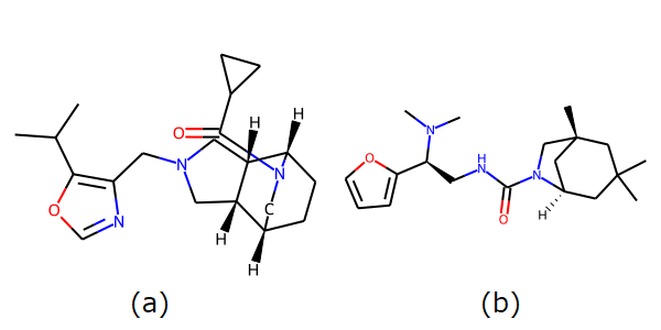
Figure 1: Two examples of structural formula in ZINC15 as drawn by RDKit. (a): A randomly chosen molecule whose ID in ZINC15 is ZINC1089752100. (b): The molecule with greatest absolute prediction error. The ID in ZINC15 is ZINC611639837.

The distribution of IGCS values is represented in the left panel of Figure 2. The most negative $\hat{\psi}_{j}$ for this molecule was $-0.0279$, for the annotated value and $-0.0310$ for the predicted value. Both of those were for feature $726$ which was absent (bit $=$ 0) for this molecule. Feature 726 was present in $955$ of the $2000$ molecules and absent in $1045$ of them. Figure 3 shows IGCS values $\hat{\psi}_{726}(t)$ letting the target $t$ be any of the $2000$ molecules. We see that very generally $\hat{\psi}_{726}$ for the true annotated values is quite close to that for the predicted values for this feature. Also, presence of the feature is strongly linked to increasing logP while absence is strongly linked to decreasing logP with perfect separation of the signs for both annotated and predicted values. The molecule ZINC10 is shown as the green circle. If bit 726 is present it typically represents the existence of a carbon chain of length three. Such a chain is denoted by ccc in the Simplified Molecular-Input Line-Entry System (SMILES) notation (Weininger,, 1988), which we also use for some other chemical features below.

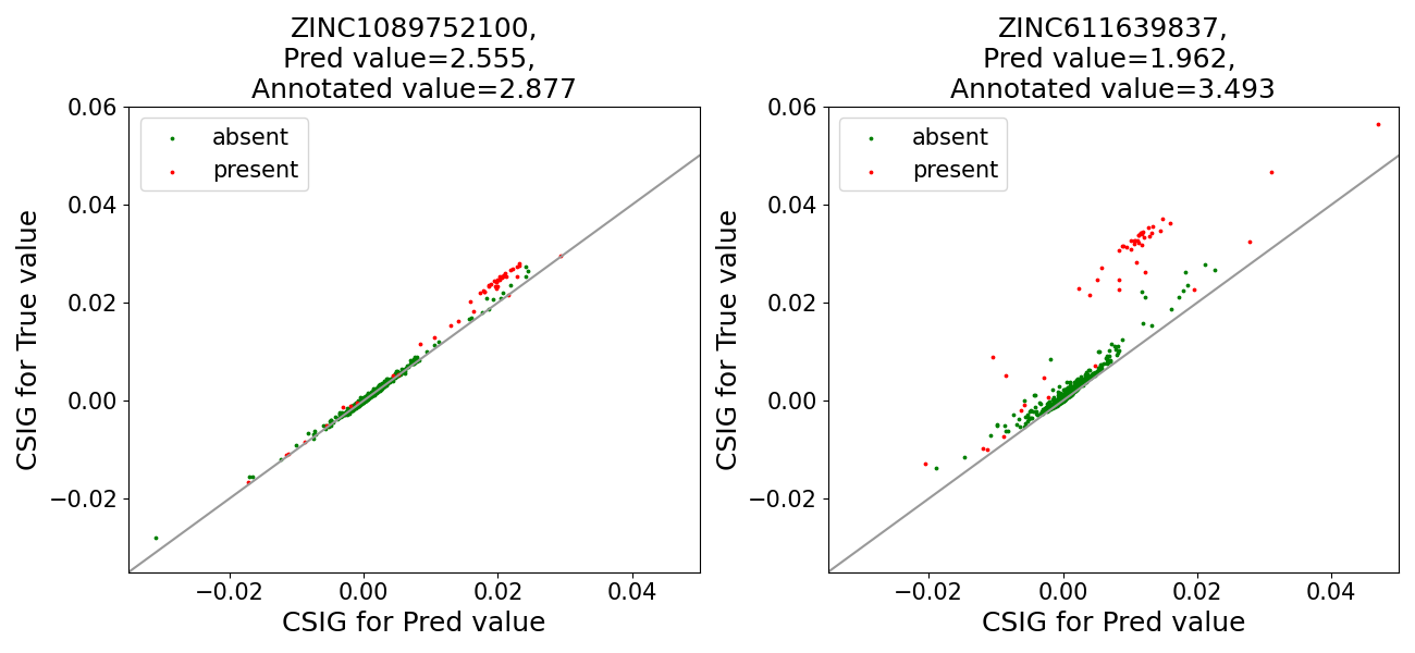
Figure 2: The contributions to the predicted value and the annotated value. Left: the molecule (a) in Figure 1. Right: the molecule (b) in Figure 1.

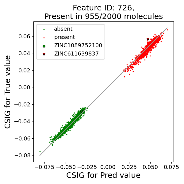
Figure 3: The distribution of IGCS assigned to feature 726 for all molecules in the dataset. The molecule of Figure 1(a) is shown as a green circle, and the one from Figure 2(b) is shown as a red triangle.

The second largest negative value for ZINC10 is $-0.0166$ for the annotated value, and $-0.0172$ for the predicted value. This comes from feature $935$ that is present in ZINC10. That feature represents the presence of Nitrogen which is known to be a water-soluble part which thus negatively contributes to logP. The corresponding Crippen value is $-0.3187$, and in this molecule there are two fragments of them so the total contribution to the annotated value is twice this Crippen value. There are three $N$ in Figure 1(a), and the one in the aromatic ring contributes $-0.3239$ to the Crippen value.

The largest positive $\hat{\psi}_{j}$ for ZINC10 is $0.0295$ for the annotated value and $0.0293$ for the predicted values. These come from feature $849$, which is present in ZINC10, representing a C–H part neighboring to the Nitrogen and the Oxygen in the aromatic ring. The corresponding Crippen value is $0.1581$.

As shown above, while the units of ECFP do not match to fragments where Crippen values are annotated and they cannot be interpreted as ground truth of XAI, the signs and rough magnitudes of Crippen values are good indicator of domain knowledge in this field and our results agree with them.

The second molecule, shown in Figure 1(b) has largest loss in the test dataset. We denote that molecule ‘ZINC61’ in this paper. Before we study the features that explain this discrepancy we remark on the features that contribute to ZINC61’s values. The two largest positive contributions to annotated value $\hat{\psi}_{j}$ are from features $726$ and $64$, the same as for ZINC10. They both come from the presence of carbon chains ccc in the aromatic ring. Because the neighboring information around those carbon chains is different, they are hashed into different features. The largest negative feature of IGCS for annotated values at ZINC61 is feature $875$ with a zero bit (absence). Feature $875$ also typically means the presence of another kind of carbon chain in the aromatic ring.

The second largest negative feature in ZINC61 feature $935$. It has the largest negative IGCS value among present features. This feature also appeared in ZINC10 as the second largest negative feature. It is about presence of N and the assigned Crippen value for this atom is $-0.3187$.

The feature where predicted importance falls short of annotated importance by the greatest amount is feature $210$. This feature is present in this molecule. Presence of feature $210$ is quite rare in the data set because only 26 of the 2000 molecules have it present. Presence is also rare for many other features. While it looks like a very rare feature, this dataset is highly sparse; about $1/4$ of the features appear in $26$ or fewer molecules. More precisely, feature 210 is the 251st ‘sparsest’ of the 1024 features. Feature $210$ in this molecule counts the presence of CCNC(N)=O (in SMILES notation). The IGCS for annotated value is $0.03160$ and for predicted value is $0.00891$. The second most underestimated feature is number $955$. It refers the presence of CNC[C@@H](c)N in this molecule. The number of molecules whose bit $955$ is one is 22, but only 4 of them corresponds to CNC[C@@H](c)N, while the other 18 molecules have presence due to hash collisions. In this sense, the various contributions should be assigned to each of the features represented in bit $955$ depending on their properties, but the limited hash length prevents it. From this viewpoint, one would have to increase the hash length of ECFP to resolve those differences.

One of the strengths of IGCS is that we can use it to identify which features are associated with a large loss between observed and predicted responses. See Figure 2(b). The vertical distance of each point from diagonal line in this figure gives a good indicator of loss SHAP, because the loss function is the usual MSE in this task. We see that the greatest source of underestimation for ZINC61 comes from the underestimation of contributions from present features. The origins of these differences can be from the sparsity of the counts of each feature over the molecules in test dataset. This kind of information must be exploited to obtain accurate models. However, there is no universal method to improve AI models. We can try feature engineering, data augmentation, modify loss function or introduce attention mechanism et cetera. This area is referred as eXplanatory Interactive machine Learning (XIL) in recent years. See Teso et al., (2022) for a review of XIL.

5.3 Number of Samples and ABC

In Section 5.1 we compared several methods in terms of ABC using the CERN data. The CS results in Section 5.1 could use exact CS because with only $d=16$ variables the cost was manageable. In the DeepChem setting it is not possible to compute CS. We are left to choose between IGCS and Monte Carlo (MC) sampling. That can be done by sampling from the $d!$ permutations underlying one expression for Shapley value or from other methods that just sample from the $d2^{d-1}$ incremental values. Sampling permutations is most straightforward because it can use uniform (unweighted) sampling. Here we compare IGCS to Monte Carlo (MC) sampling via ABC. The IGCS values will have a bias because $\psi_{j}\neq\phi_{j}$. MC estimates $\hat{\phi}_{j}$ are unbiased but can have high variance.

A comparison is made in Table 5 and illustrated in Figure 4. The averages are over 2000 held out molecules. The error bars represent $\pm 1$ standard error. This is a standard error over the 2000 molecules not over the MC simulations. The results are compared to IGCS with two choices for the number of function values in the Riemann sum. The IGCS reference lines are surrounded by bands shading plus or minus one standard error (over 2000 molecules) of the IGCS values.

The MC estimates show a clear upward trend; as more MC samples are taken, the estimated ABCs trend steadily upwards. While the underlying MC $\hat{\phi}_{j}$ are unbiased, the ABC estimates apply a nonlinear variable ranking transformation to those estimates so that the MC-based estimates $\widehat{\mathrm{ABC}}$ are biased. From Figure 4 it is evident that truly enormous MC sampling cost would be required for the MC-based method to get ABC scores comparable to those of IGCS. MC sampling with about the same cost in time as IGCS using $50$ gradient points to estimate the integral yields an insertion ABC of $0.052$ compared to $0.149$ with half a million Monte Carlo samples. When ABC methods are used to demonstrate a good ordering, we can see that MC can have severe difficulty.

Number of	Insertion ABC	Deletion ABC	Time
Samples	(Std. error)	(Std. error)	(sec./data)
2049	0.052 (0.016)	0.063 (0.016)	0.517
10000	0.028 (0.017)	0.037 (0.017)	1.387
100000	0.071 (0.016)	0.060 (0.017)	14.760
200000	0.106 (0.015)	0.114 (0.016)	29.154
300000	0.128 (0.014)	0.144 (0.015)	44.720
400000	0.146 (0.014)	0.169 (0.015)	59.618
500000	0.149 (0.014)	0.179 (0.015)	74.503
50 steps IGCS	0.318 (0.010)	0.637 (0.011)	0.516
200 steps IGCS	0.330 (0.010)	0.664 (0.011)	0.661

Table 5: The ABCs with different sampling number in CS and IGCS of ZINC15 data. The numbers in the parenthesis represent the standard error in 2000 data.

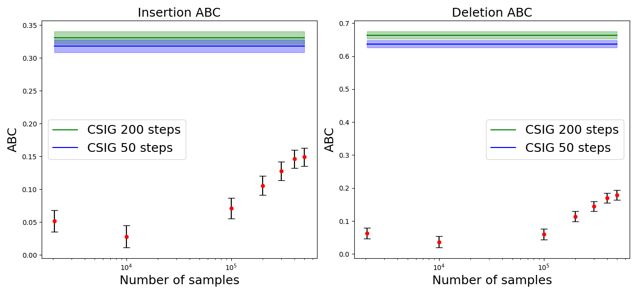
Figure 4: The ABCs with different sampling number in CS of ZINC15.

The computation time is measured in a server with Intel(R) Xeon(R) Gold 6132 CPU @ 2.60GHz and Tesla V100-SXM2.

6 Conclusion

We have introduced a new variable importance measure, IGCS, based on Aumann-Shapley theory. Like CS it is model-free, but unlike CS it can easily scale to high dimensional settings without incurring exponential cost. IGCS has a value function on $[0,1]^{d}$ that is essentially multilinear over all but a negligible portion of the unit cube when $d\gg\log(n)$. That then makes it close to CS in the high dimensional settings where exponential cost rules out exact CS computations. The disadvantage of IGCS is the same as CS: the user needs to define what it means for two levels of a variable to be similar. While this is a burden for non-binary variables, a user-defined notion of similarity is more transparent than having a notion of similarity that emerges from some other black box.

This model-free method is useful in settings where the prediction function $f$ is not available either because it is proprietary or because it is prohibitively expensive. It can also be used on raw data or on residuals from a model.

Appendix A Detailed Model Descriptions

This appendix provides some background details on the experiments conducted in this article.

A.1 CERN Electron Collision Data

The hyperparameters for the model used in Section 5.1.1 are given in Table 6. They were obtained from a hyperparameter search using Optuna from Akiba et al., (2019). Each intermediate layer is a parametric ReLU with dropout. The dropout ratio is common to all of the layers. The model is trained with Huber loss. The model is overall very accurate but the very highest values are systematically underestimated, as seen in Hama et al., (2022) which also used this model.

Hyperparameter	Value
Dropout Ratio	0.11604
Learning Rate	$1.9163\times 10^{-4}$
Number of Neurons	[509–421–65–368–122–477]
Huber Parameter	$1.0$

Table 6: Parameters of the MLP model for the CERN Electron Collision Data.

A.2 ZINC15 Data

The model used in Section 5.2 is trained with RobustMultitaskRegressor of Ramsundar et al., (2017) by three tasks annotated in ZINC15 in DeepChem. The model is trained with mean squared loss. The hyperparameters for the model are given in Table 7. The number of nodes in a hidden layer is determined from a search using Optuna from Akiba et al., (2019). The learning rate is exponentially decaying from $0.01$ with a decay rate of $0.8$ per $1000$ steps.

Hyperparameter	Value
Dropout Ratio	0.25
Number of Neurons in a hidden layer	[3935]

Table 7: Parameters of the MLP model that estimate logP values in ZINC15 from ECFP vectors.

Appendix B Empirical Gaussian Kernel Weight

Here, we describe our modification of the Gaussian kernel weight (GKW) method that we used in Section 5. The Gaussian kernel weight method of Aas et al., (2021) is not model free. Here we describe a model-free adaptation of it.

The value function in GKW takes the form

$$\nu(u)=\frac{\sum_{i=1}^{n}s_{u}(\bm{x}_{i},\bm{x}_{t})f(\bm{x}_{i,u}{:}\bm{x}_{t,-u})}{\sum_{i=1}^{n}s_{u}(\bm{x}_{i},\bm{x}_{t})}$$ (8)

for a weight function

$$s_{u}(\bm{x}_{i},\bm{x}_{t})=\exp\left(-\frac{D_{u}^{2}(\bm{x}_{i},\bm{x}_{t})}{2\sigma^{2}}\right)$$

where

$$D_{u}(\bm{x}_{i},\bm{x}_{t})=\sqrt{\frac{(\bm{x}_{i,u}-\bm{x}_{t,u})^{\mathsf{T}}\Sigma_{uu}^{-1}(\bm{x}_{i,u}-\bm{x}_{t,u})}{|u|}}.$$

The function $D_{u}$ is a scaled Mahalanobis distance from $\bm{x}_{iu}$ to $\bm{x}_{tu}$. It uses $\Sigma_{uu}$ which is the $|u|\times|u|$ covariance matrix among the $\bm{x}_{iu}$ values. The distances and weights are measured in data space, not in indicator space, so they are available for real-valued features but perhaps not for other features.

GKW has a parameter $\sigma>0$. The authors of Aas et al., (2021) recommend choosing it via AIC. That is expensive and they also report that a default such as $\sigma=0.1$ works well in practice.

Before modifying GKW we make two observations. First, the normalization by $|u|$ within $D_{u}$ is unusual and it means that the distance from $\bm{x}_{iu}$ to $\bm{x}_{tu}$ could actually decrease when we incorporate another variable, replacing $u$ by $u\cup\{j\}$. We are not able to say whether this is a strength or weakness of GKW, just that it is an interesting propoerty. Second, the value $\sigma=0.1$ gave us some concern. It makes $s_{u}(\bm{x}_{i},\bm{x}_{t})$ equal to $\exp(-50S^{2}_{u})$ where $S^{2}_{u}$ is a standardized mean square difference. It seems that this would then put the vast majority of the weight on the single closest point to $\bm{x}_{t}$, namely $\bm{x}_{t}$ itself. To address this concern we tried a larger values of $\sigma$ ($1.0$ and $10.0$) and found them to perform worse than $\sigma=0.1$ in our adaptation and so we work with the recommended default.

The GKW formula (8) is of interventional type. It uses hybrid points that are not observed. This means it cannot be used in a model-free setting. It may also reference impossible input combinations. We replace the hybrid points in (8) by observed data points, getting

$$\nu(u)=\frac{\sum_{i=1}^{n}s_{u}(\bm{x}_{i},\bm{x}_{t})f(\bm{x}_{i})}{\sum_{i=1}^{n}s_{u}(\bm{x}_{i},\bm{x}_{t})}.$$ (9)

We are then able to derive Shapley values from this model-free measure.

Appendix C Higher Order Taylor Expansion

We saw in Section 4 that for the overwhelming majority of the unit cube $[0,1]^{d}$ and of its corners $\{0,1\}^{d}$, the Taylor expansion (4) of the CSIG function is convergent. The first order term is one where integrated gradients give the same values as Shapley. It is then instructive to carry out the Taylor expansion to one more term to see how a mismatch between CS and IGCS arises. Doing that we get

$$\nu(\bm{z}) \approx f(\bm{x}_{t})+\sum_{i\neq t}f(\bm{x}_{i})\prod_{j\in J_{i}}(1-z_{j})-f(\bm{x}_{t})\sum_{i\neq t}\prod_{j\in J_{i}}(1-z_{j})$$

$$\quad-\sum_{i\neq t}f(\bm{x}_{i})\sum_{i^{\prime}\neq t}\prod_{j\in J_{i}}(1-z_{j})\prod_{j\in J_{i^{\prime}}}(1-z_{j}).$$

There are two new terms. The first new term also involves products over $j\in J_{i}$ of $1-z_{j}$ and so it also is one for which IGCS matches CS.

The second new term need not be of that form. It does however involve two such products of factors $1-z_{j}$ and we know that each such product is typically smaller than $\epsilon$. That term is then $O(n^{2}\epsilon^{2})$ over most of $[0,1]^{d}$ while the other terms are $O(n\epsilon)$. For large $d$ it is easy to make $n\epsilon$ negligible. For instance with $\epsilon=1/n^{2}$ we get $\Pr(\bm{z}\in H_{\epsilon})\leqslant n^{4}\exp(-\lfloor ad\rfloor/4)$. This is negligible for $d\gg(16/a)\log(n)$.

The second new term is a weighted sum of

$$g_{i,i^{\prime}}(\bm{z})=\prod_{j\in J_{i}}(1-z_{j})\prod_{j\in J_{i^{\prime}}}(1-z_{j})=\prod_{j\in J_{i}\cap J_{i^{\prime}}}(1-z_{j})\times\prod_{j\in J_{i}\cup J_{i^{\prime}}}(1-z_{j}).$$

It is the factors $j\in J_{i}\cap J_{i^{\prime}}$ that make IGCS differ from CS. The cohort Shapley value for $g_{i,i^{\prime}}$ is

$$\frac{1}{|J_{i}\cup J_{i^{\prime}}|}\times 1\{j\in J_{i}\cup J_{i^{\prime}}\}.$$

This follows from symmetry and the fact that $g_{i,i^{\prime}}$ only takes values $0$ or $1$ at the corners of the cube.

To find the IGCS value for $g_{i,i^{\prime}}$, note that

$$g_{i,i^{\prime}}(\bm{z}) =\prod_{j\in J_{i}\cap J_{i^{\prime}}}(1-z_{j})^{2}\prod_{j\in J_{i}\triangle J_{i^{\prime}}}(1-z_{j})$$

where $\triangle$ denotes the symmetric difference. For $j^{\prime}\in J_{i}\cap J_{i^{\prime}}$

$$\frac{\partial}{\partial z_{j^{\prime}}}g_{i,i^{\prime}}(\bm{z}) =-2\prod_{j\in J_{i}\cap J_{i^{\prime}}\setminus\{j^{\prime}\}}(1-z_{j})^{2}\prod_{j\in J_{i}\triangle J_{i^{\prime}}\cup\{j^{\prime}\}}(1-z_{j}),\quad\text{so}$$

$$\frac{\partial}{\partial z_{j^{\prime}}}g_{i,i^{\prime}}(z\bm{1}) =-2(1-z)^{2|J_{i}\cap J_{i^{\prime}}|+|J_{i}\triangle J_{i^{\prime}}|-1}$$

which has IGCS value

$$\frac{2}{2|J_{i}\cap J_{i^{\prime}}|+|J_{i}\triangle J_{i^{\prime}}|}.$$

Similarly for $j^{\prime}\in J_{i}\triangle J_{i^{\prime}}$

$$\frac{\partial}{\partial z_{j^{\prime}}}g_{i,i^{\prime}}(\bm{z}) =-1\prod_{j\in J_{i}\cap J_{i^{\prime}}}(1-z_{j})^{2}\prod_{j\in J_{i}\triangle J_{i^{\prime}}\setminus\{j^{\prime}\}}(1-z_{j}),\quad\text{so}$$

$$\frac{\partial}{\partial z_{j^{\prime}}}g_{i,i^{\prime}}(z\bm{1}) =-(1-z)^{2|J_{i}\cap J_{i^{\prime}}|+|J_{i}\triangle J_{i^{\prime}}|-1}$$

which has IGCS value

$$\frac{1}{2|J_{i}\cap J_{i^{\prime}}|+|J_{i}\triangle J_{i^{\prime}}|}.$$

The consequence is that IGCS gives extra weight to $j\in J_{i}\cup J_{i^{\prime}}$ and less to $j\in J_{i}\triangle J_{i^{\prime}}$. We expect that any given variable $j$ will be in the double weight grouping for some pairs $i,i^{\prime}$ and in the single weight grouping for others. A variable $j$ where $x_{ij}$ is rarely dissimilar to $x_{tj}$ is less likely to get those double weightings.

The above argument has not used the full generality of Corollary 1. Approximation within the wider class of functions considered there can only reduce the differences $|\psi_{j}-\phi_{j}|$ between IGCS and CS compared to the multilinear functions in our Taylor expansion.

Appendix D Deletion and Insertion Measures

As noted earlier, there is no ground truth for variable importance. Instead there are multiple definitions of what makes a variable important and choosing a definition involves some tradeoffs. It is however possible to compute the value of a proxy measure derived from an area under the curve (AUC) quantity defined by Petsiuk et al., (2018). Our presentation of that measure is based on the analysis of AUC in Hama et al., (2022).

The proxy measure is about the quality with which the variables’ importances can be ranked. For an interventional method like baseline Shapley, the quality of a ranking can be measured as follows. We sort the variables from those with the largest $\phi_{j}$ to those with the smallest $\phi_{j}$. For $k=0,1,\dots,d$ let $\tilde{\bm{x}}_{k}$ be a hybrid point with $\tilde{x}_{kj}=x_{tj}$ if variable $j$ is among the $k$ variables with the largest $\phi_{j}$ and let $\tilde{x}_{kj}=x_{bj}$ otherwise. Then let $\tilde{y}_{k}=f(\tilde{\bm{x}}_{k})$ and consider the piecewise linear curve going through the points $(k,\tilde{y}_{k})$ over the interval $[0,d]$. The AUC criterion is the (signed) area under this curve. If the variables have been well ranked then the AUC of the insertion curve will be large. Hama et al., (2022) describe an area between the curves (ABC) that subtracts the area under a straight line connecting $(0,\tilde{y}_{0})$ to $(d,\tilde{y}_{k})$. If one method has a better AUC than another it will also have a better ABC. That paper argues that ABC is better suited to regression problems than AUC which was devised for classification.

There is a similar deletion curve found by changing the variables in the reverse order. Hama et al., (2022) define an ABC for deletion as the signed area under the straight line minus the area under the deletion curve.

Ranking is not the same as estimating the $\phi_{j}$. Hama et al., (2022) show an example where ranking by the true Shapley values can give a lesser ABC than some other ranking. They also show that for certain simple models, such as logistic regression and naive Bayes, that ranking by Shapley value does indeed maximize the ABC. Since those models often perform well, we expect that more sophisticated models will often make similar predictions and then ABC will be a useful scorecard.

On our data examples it is impossible to compute the true Shapley values so we use ABC measures as a guide to compare CS to IGCS and some other methods.

Just as there is more than one way to define variable importance, there is more than one way to define an ABC measure to rank variable importance measures. Instead of the interventional approach above one can replace $\tilde{y}_{k}$ by the average value of $f(\bm{x}_{i})$ over the cohort of points that are similar to $\bm{x}_{t}$ for the $k$ variables with the greatest value of $\phi_{j}$. This provides a conditional ABC measure as an alternative to an interventional ABC measure.

We expect on intuitive grounds that a method which attempts to compute interventional Shapley values will attain a better interventional ABC value than one that attempts to compute conditional Shapley values and vice versa. While we do not prove that this must happen, it did happen in our numerical examples. We have a strong preference to avoid interventional measures as they can require evaluating $f$ at some wildly unrealistic input values, but other researchers might accept those measures.

References

- Aas et al., (2021) Aas, K., Jullum, M., and Løland, A. (2021). Explaining individual predictions when features are dependent: More accurate approximations to Shapley values. Artificial Intelligence, 298:103502.
- Ahn et al., (2023) Ahn, S., Grana, J., Tamene, Y., and Holsheimer, K. (2023). Local model explanations and uncertainty without model access. Technical report, arXiv:2301.05761.
- Akiba et al., (2019) Akiba, T., Sano, S., Yanase, T., Ohta, T., and Koyama, M. (2019). Optuna: A next-generation hyperparameter optimization framework. In Proceedings of the 25th ACM SIGKDD international conference on knowledge discovery & data mining, pages 2623–2631.
- Angwin et al., (2016) Angwin, J., Larson, J., Mattu, S., and Kirchner, L. (2016). Machine bias: there’s software used across the country to predict future criminals. and it’s biased against blacks.
- Aumann and Shapley, (1974) Aumann, R. J. and Shapley, L. S. (1974). Values of Non-Atomic Games. Princeton University Press, Princeton, NJ.
- Azadkia and Chatterjee, (2021) Azadkia, M. and Chatterjee, S. (2021). A simple measure of conditional dependence. The Annals of Statistics, 49(6):3070–3102.
- Chen et al., (2022) Chen, H., Lundberg, S. M., and Lee, S.-I. (2022). Explaining a series of models by propagating Shapley values. Nature communications, 13(1):1–15.
- Dawid and Musio, (2021) Dawid, A. P. and Musio, M. (2021). Effects of causes and causes of effects. Annual Review of Statistics and Its Application, 9.
- Friedman, (2004) Friedman, E. J. (2004). Paths and consistency in additive cost sharing. International Journal of Game Theory, 32:501–518.
- Frye et al., (2020) Frye, C., de Mijolla, D., Begley, T., Cowton, L., Stanley, M., and Feige, I. (2020). Shapley explainability on the data manifold. arXiv preprint arXiv:2006.01272.
- Hama et al., (2022) Hama, N., Mase, M., and Owen, A. B. (2022). Deletion and insertion tests in regression models. arXiv preprint arXiv:2205.12423.
- Heberle et al., (2022) Heberle, H., Zhao, L., Schmidt, S., Wolf, T., and Heinrich, J. (2022). XSMILES: interactive visualization for molecules, SMILES and XAI scores. Research Square preprint.
- Herin et al., (2022) Herin, M., Idrissi, M. I., Chabridon, V., and Iooss, B. (2022). Proportional marginal effects for global sensitivity analysis. Technical report, arXiv:2210.13065.
- Hooker and Mentch, (2019) Hooker, G. and Mentch, L. (2019). Please stop permuting features: An explanation and alternatives. arXiv e-prints, pages arXiv–1905.
- Hooker et al., (2018) Hooker, S., Erhan, D., Kindermans, P.-J., and Kim, B. (2018). A benchmark for interpretability methods in deep neural networks. arXiv preprint arXiv:1806.10758.
- Kumar et al., (2020) Kumar, I. E., Venkatasubramanian, S., Scheidegger, C., and Friedler, S. (2020). Problems with Shapley-value-based explanations as feature importance measures. In Proceedings of the 37th International Conference on Machine Learning (ICML 2020).
- Laurent and Massart, (2000) Laurent, B. and Massart, P. (2000). Adaptive estimation of a quadratic functional by model selection. Annals of Statistics, pages 1302–1338.
- Lindeman et al., (1980) Lindeman, R. H., Merenda, P. F., and Gold, R. Z. (1980). Introduction to bivariate and multivariate analysis. Scott, Foresman and Company, Homewood, IL.
- Lundberg and Lee, (2017) Lundberg, S. and Lee, S.-I. (2017). A unified approach to interpreting model predictions. arXiv preprint arXiv:1705.07874.
- Lundberg et al., (2020) Lundberg, S. M., Erion, G., Chen, H., DeGrave, A., Prutkin, J. M., Nair, B., Katz, R., Himmelfarb, J., Bansal, N., and Lee, S.-I. (2020). From local explanations to global understanding with explainable AI for trees. Nature machine intelligence, 2(1):56–67.
- Mase et al., (2019) Mase, M., Owen, A. B., and Seiler, B. (2019). Explaining black box decisions by Shapley cohort refinement. Technical report, arXiv:1911.00467.
- Mase et al., (2021) Mase, M., Owen, A. B., and Seiler, B. B. (2021). Cohort Shapley value for algorithmic fairness. Technical report, arXiv:2105.07168.
- Mase et al., (2024) Mase, M., Owen, A. B., and Seiler, B. B. (2024). Variable importance without impossible data. Annual Review of Statistics and its Application. (to appear).
- McCauley, (2014) McCauley, T. (2014). Events with two electrons from 2010. CERN Open Data Portal.
- Molnar, (2018) Molnar, C. (2018). Interpretable machine learning: A Guide for Making Black Box Models Explainable. Leanpub.
- Owen, (1972) Owen, G. (1972). Multilinear extensions of games. Management Science, 18(5-part-2):64–79.
- Petsiuk et al., (2018) Petsiuk, V., Das, A., and Saenko, K. (2018). RISE: Randomized input sampling for explanation of black-box models. arXiv preprint arXiv:1806.07421.
- Ramsundar et al., (2019) Ramsundar, B., Eastman, P., Walters, P., Pande, V., Leswing, K., and Wu, Z. (2019). Deep Learning for the Life Sciences. O’Reilly Media. https://www.amazon.com/Deep-Learning-Life-Sciences-Microscopy/dp/1492039837.
- Ramsundar et al., (2017) Ramsundar, B., Liu, B., Wu, Z., Verras, A., Tudor, M., Sheridan, R. P., and Pande, V. (2017). Is multitask deep learning practical for pharma? Journal of chemical information and modeling, 57(8):2068–2076.
- Razavi et al., (2021) Razavi, S., Jakeman, A., Saltelli, A., Prieur, C., Iooss, B., Borgonovo, E., Plischke, E., Piano, S. L., Iwanaga, T., Becker, W., Tarantola, S., Guillaume, J. H. A., Jakeman, J., Gupta, H., Milillo, N., Rabitti, G., Chabridon, V., Duan, Q., Sun, X., Smith, S., Sheikholeslami, R., Hosseini, N., Asadzadeh, M., Puy, A., Kucherenko, S., and Maier, H. R. (2021). The future of sensitivity analysis: An essential discipline for systems modeling and policy support. Environmental Modelling & Software, 137:104954.
- Rényi, (1959) Rényi, A. (1959). On measures of dependence. Acta Mathematica Hungarica, 10(3-4):441–451.
- Rogers and Hahn, (2010) Rogers, D. and Hahn, M. (2010). Extended-connectivity fingerprints. Journal of chemical information and modeling, 50(5):742–754.
- Rudin, (2019) Rudin, C. (2019). Stop explaining black box machine learning models for high stakes decisions and use interpretable models instead. Nature Machine Intelligence, 1(5):206–215.
- Seiler et al., (2023) Seiler, B. B., Mase, M., and Owen, A. B. (2023). What makes you unique? Electronic Journal of Statistics, 17(1):1–8.
- Shapley, (1953) Shapley, L. S. (1953). A value for n-person games. In Kuhn, H. W. and Tucker, A. W., editors, Contribution to the Theory of Games II (Annals of Mathematics Studies 28), pages 307–317. Princeton University Press, Princeton, NJ.
- Sterling and Irwin, (2015) Sterling, T. and Irwin, J. J. (2015). ZINC 15–ligand discovery for everyone. Journal of chemical information and modeling, 55(11):2324–2337.
- Sun and Sundararajan, (2011) Sun, Y. and Sundararajan, M. (2011). Axiomatic attribution for multilinear functions. In Proceedings of the 12th ACM conference on Electronic commerce, pages 177–178.
- Sundararajan and Najmi, (2020) Sundararajan, M. and Najmi, A. (2020). The many Shapley values for model explanation. In International Conference on Machine Learning, pages 9269–9278. PMLR.
- Sundararajan et al., (2017) Sundararajan, M., Taly, A., and Yan, Q. (2017). Axiomatic attribution for deep networks. In International Conference on Machine Learning, pages 3319–3328. PMLR.
- Székely and Rizzo, (2013) Székely, G. J. and Rizzo, M. L. (2013). Energy statistics: A class of statistics based on distances. Journal of statistical planning and inference, 143(8):1249–1272.
- Tamura et al., (2021) Tamura, S., Jasial, S., Miyao, T., and Funatsu, K. (2021). Interpretation of ligand-based activity cliff prediction models using the matched molecular pair kernel. Molecules, 26(16):4916.
- Teso et al., (2022) Teso, S., Alkan, Ö., Stammer, W., and Daly, E. (2022). Leveraging explanations in interactive machine learning: An overview. arXiv preprint arXiv:2207.14526.
- Wei et al., (2015) Wei, P., Lu, Z., and Song, J. (2015). Variable importance analysis: A comprehensive review. Reliability Engineering & System Safety, 142:399–432.
- Weininger, (1988) Weininger, D. (1988). SMILES, a chemical language and information system. 1. introduction to methodology and encoding rules. Journal of chemical information and computer sciences, 28(1):31–36.
- Wildman and Crippen, (1999) Wildman, S. A. and Crippen, G. M. (1999). Prediction of physicochemical parameters by atomic contributions. Journal of chemical information and computer sciences, 39(5):868–873.
- Zhang and Janson, (2020) Zhang, L. and Janson, L. (2020). Floodgate: inference for model-free variable importance. Technical report, arXiv:2007.01283.