Using multimodal learning and
deep generative models
for corporate bankruptcy prediction

ABSTRACT

Textual data from financial filings, e.g., the Management’s Discussion & Analysis (MDA) section in Form 10-K, has been used to improve the prediction accuracy of bankruptcy models. In practice, however, we cannot obtain the MDA section for all public companies. The two main reasons for the lack of MDA are: (i) not all companies are obliged to submit the MDA and (ii) technical problems arise when crawling and scrapping the MDA section. This research introduces for the first time, to the best of our knowledge, the concept of multimodal learning in bankruptcy prediction models to solve the problem that for some companies we are unable to obtain the MDA text. We use the Conditional Multimodal Discriminative (CMMD) model to learn multimodal representations that embed information from accounting, market, and textual modalities. The CMMD model needs a sample with all data modalities for model training. At test time, the CMMD model only needs access to accounting and market modalities to generate multimodal representations, which are further used to make bankruptcy predictions. This fact makes the use of bankruptcy prediction models using textual data realistic and possible, since accounting and market data are available for all companies unlike textual data. The empirical results in this research show that the classification performance of our proposed methodology is superior compared to that of a large number of traditional classifier models. We also show that our proposed methodology solves the limitation of previous bankruptcy models using textual data, as they can only make predictions for a small proportion of companies.

Keywords: Bankruptcy prediction, MD&A, Form 10-K, Multimodal Learning, Deep Generative Models, Textual data, Representation Learning

1 Introduction

Corporate bankruptcy prediction plays an important role for both regulators and analysts in the financial industry (Ding et al., 2012). Therefore, there is a vast body of literature on bankruptcy models (see Table 1), which mostly use panel data containing accounting and market information to predict whether a company will fall into financial distress. Most recently, textual data from financial filings, such as the Management’s Discussion & Analysis (MDA) section of Form 10-K, has been used to improve the prediction accuracy of bankruptcy models, e.g. Cecchini et al. (2010); Mayew et al. (2015); Mai et al. (2019) and Kim and Yoon (2021), as it provides a forward-looking view of the company’s performance. The information contained in the MDA section has also been used in other research domains, e.g., forecasting corporate investment (Cho and Muslu, 2021; Berns et al., 2022) or financial events (Cecchini et al., 2010), spillover effects (Durnev and Mangen, 2020), or in tax avoidance (Zhang et al., 2022), just to name a few. In all cases the MDA section has proven to contain valuable information.

Traditional methods for corporate bankruptcy prediction require that the same data are used during model training to make a new bankruptcy prediction. Unfortunately, for models using the MDA section this is not always possible. While it is true that the financial regulator requires a wealth of information in the company’s annual reports on Form 10-K, not all companies are obliged to fulfill this requirement. Additionally, obtaining the MDA section for statistical modeling involves technical procedures (Web crawling and scraping) that do not guarantee a successful extraction. As a consequence, using textual data in bankruptcy models to develop relatively more accurate models is not feasible in practice, since financial regulators or investors are not able to make bankruptcy predictions for all companies.

This research introduces a novel methodology for bankruptcy prediction, which is based on multimodal learning and uses the Conditional MultiModal Discriminative (CMMD) model introduced in Mancisidor et al. (2021). Under the CMMD framework, accounting (${\bm{x}}_{1}$), market (${\bm{x}}_{2}$), and textual data (${\bm{x}}_{3}$) are considered data modalities that provide different information about the financial condition of a given company. Further, the CMMD framework assumes that accounting and market modalities are always observed, i.e., $\bm{x}_{\scriptstyle\scriptscriptstyle\mathcal{O}}=({\bm{x}}_{1},{\bm{x}}_{2})$. On the other hand, textual data $\bm{x}_{\scriptstyle\scriptscriptstyle\mathcal{M}}={\bm{x}}_{3}$ and class labels $y$ are available for model training but missing at test time. After optimization of the objective function, the CMMD model embeds information from all data modalities ($\bm{x}_{\scriptstyle\scriptscriptstyle\mathcal{O}}$ and $\bm{x}_{\scriptstyle\scriptscriptstyle\mathcal{M}}$) into a multimodal data representation (${\bm{z}}$). The new representation ${\bm{z}}$ of the data modalities is believed to be capable of capturing the posterior distribution of the explanatory factors of the data modalities $\bm{x}_{\scriptstyle\scriptscriptstyle\mathcal{O}}$ and $\bm{x}_{\scriptstyle\scriptscriptstyle\mathcal{M}}$, and is therefore useful as input to a classifier model (Bengio et al., 2013). Hence, the CMMD model can predict corporate bankruptcy using multimodal representations ${\bm{z}}$, instead of the accounting, market, and textual data themselves.

The CMMD model requires all data modalities and class labels only during model training. At test time, CMMD generates multimodal representations ${\bm{z}}$ for a new company simply by using $\bm{x}_{\scriptstyle\scriptscriptstyle\mathcal{O}}$, i.e., accounting and market data. This is possible by minimizing a divergence measure between a prior distribution $p({\bm{z}}|\bm{x}_{\scriptstyle\scriptscriptstyle\mathcal{O}})$ (conditioned on the always observed data modalities) and a posterior distribution $q({\bm{z}}|\bm{x}_{\scriptstyle\scriptscriptstyle\mathcal{O}},\bm{x}_{\scriptstyle\scriptscriptstyle\mathcal{M}},y)$ (conditioned on all data modalities and class labels). Such minimization has the effect of bringing the prior close to the posterior (Suzuki et al., 2016), and it also minimizes the expected information required to convert a sample from the prior into a sample from the posterior distribution (Doersch, 2016). Using multimodal representations ${\bm{z}}\sim p({\bm{z}}|\bm{x}_{\scriptstyle\scriptscriptstyle\mathcal{O}})$ for bankruptcy prediction, and not the data modalities $\bm{x}_{\scriptstyle\scriptscriptstyle\mathcal{O}}$ and $\bm{x}_{\scriptstyle\scriptscriptstyle\mathcal{M}}$ themselves, has therefore one main advantage. That is, the CMMD model avoids the limitation of previous bankruptcy models since CMMD does not require the information contained in $\bm{x}_{\scriptstyle\scriptscriptstyle\mathcal{M}}$ to be available for making new bankruptcy predictions.

Using data from companies listed on the AMEX, NYSE and NASDAQ stock exchanges the empirical results of this research show that for relatively large training data sets, our proposed methodology achieves higher classification performance compared to traditional classifiers, which use accounting and market modalities to make bankruptcy predictions. 40% of the companies in our data sample lack MDA for one of the reasons explained above, meaning that traditional classifiers that use all three data modalities can only make bankruptcy predictions for 60% of the companies. On the contrary, our proposed methodology for bankruptcy prediction, which only use accounting and market modalities to generate multimodal representations, may be used for all companies. To summarize, our main contributions are:

• We introduce for the first time, to the best of our knowledge, the concept of multimodal learning for corporate bankruptcy models.

• We resolve the limitation of previous bankruptcy models that require MDA data to make predictions, as they can only make predictions for a proportion of firms that is significantly smaller than the number it would need to be in reality. This makes the use of MDA data realistic and possible.

2 Related Work

Since the seminal work of Beaver (1966) and Altman (1968) on corporate bankruptcy prediction, research in this field has grown rapidly over the past 50 years. Therefore, this section focuses on the application of neural networks and textual data for bankruptcy prediction. For an exhaustive review on other bankruptcy prediction models, the reader is referred to Kumar and Ravi (2007); Demyanyk and Hasan (2010) and Alaka et al. (2018).

The use of neural networks (NNs) in bankruptcy prediction dates back to 1990 with the research by Bell et al. (1990) and Odom and Sharda (1990). The authors compare the relative performance of NNs over logistic regression (LR) and multivariate discriminant analysis (DA), respectively. In both cases, the architecture of the NN is simple. Bell et al. (1990) use one hidden layer with 6 neurons, while Odom and Sharda (1990) use 5 neurons in the hidden layer. In both cases, NNs are optimized with the backpropagation algorithm (Rumelhart et al., 1985). The results in these pioneering studies are contradictory; NNs show no significant improvement over LR (Bell et al., 1990), but outperform DA in predicting bankruptcy (Odom and Sharda, 1990).

Table 1: Research on bankruptcy prediction with neural networks. The column ”Benchmark models” includes the following abbrevations: logistic regression (LR), probit regression (PR), discriminant analysis (DA), linear classifier (LC), k-nearest neighbors (kNN), decision trees (DT), random forest (RF), probabilistic neural networks (PNN), self organizing maps (SOM), genetic algorithm (GA), generalized additive models (GAM), ensemble models (EM), fuzzy neural networks (FNN), stacked generalization model (SGM), support vector machine (SVM), leave-one-out incremental extreme learning machine (LOO-IELM), deep learning (DL).

(Year)   Author Benchmark Models No. obs. No. bankruptcies Period No. years (1990) Bell et al. (Bell et al., 1990) LR 2067 233 1985-1986 2 (1990) Odom and Sharda (Odom and Sharda, 1990) DA 129 65 1975-1982 8 (1992) Tam and Kiang (Tam and Kiang, 1992) DA, LC, LR, kNN, and DT 162 81 1985-1987 3 (1992) Salchenberger et al. (Salchenberger et al., 1992) LR 316, 404 158, 75 1986-1987 2 (1993) Chung and Tam (Chung and Tam, 1993) DA, LR, DT 162 81 1985-1987 3 (1993) Coats and Fant (Coats and Fant, 1993) DA 282 94 1970-1989 20 (1993) Fletcher and Goss (Fletcher and Goss, 1993) LR 36 18 1971-1979 9 (1994) Wilson and Sharda (Wilson and Sharda, 1994) DA 129 65 1975-1982 8 (1994) Fanning and Cogger (Fanning and Cogger, 1994) LR 380 190 1942-1965 24 (1995) Boritz et al. (Boritz et al., 1995) DA, LR, PR 6324 171 1971-1984 14 (1997) Etheridge and Sriram (Etheridge and Sriram, 1997) DA, LR 1139 148 1986-1988 3 (1997) Barniv et al. (Barniv et al., 1997) DA, LR 237 69 1980-1991 12 (1997) Jain and Nag (Jain and Nag, 1997) LR 431 327 1976-1988 13 (1999) Yang et al. (Yang et al., 1999) DA, PNN 122 33 1984-1989 6 (1999) Zhang et al. (Zhang et al., 1999) LR 220 110 1980-1991 12 (2001) Atiya Atiya (2001) - 1160 444 - - (2005) Lee et al. (Lee et al., 2005) SOM, DA, LR 168 84 1995-1998 4 (2005) Pendharkar (Pendharkar, 2005) DA, GA, DT 200 100 1987-1995 9 (2006) Neves and Vieira (Neves and Vieira, 2006) DA 2800 583 1998-2000 3 (2006) Ravikumar and Ravi (Ravikumar and Ravi, 2006) - 129 65 - - (2006) Berg (Berg, 2007) GAM, DA, - - 1996-2000 5 (2008) Tsai and Wu (Tsai and Wu, 2008) EM 690, 1000, 360 383, 300, 383 - - (2008) Alfaro et al. (Alfaro et al., 2008) EM, DA, DT 1180 590 2000-2003 4 (2008) Ravi and Pramodh (Ravi and Pramodh, 2008) - 66, 40 - - - (2008) Huang (Huang, 2008) FNN 400 80 2002-2005 4 (2009) Chauhan et al. (Chauhan et al., 2009) WNN, DEWNN, TAWNN 40, 66, 129 22, 37, 65 - - (2010) Kim and Kang (Kim and Kang, 2010) EM 1458 729 2002-2005 4 (2010) Cecchini et al. (Cecchini et al., 2010) - 156 78 1994-1999 6 (2012) Jeong et al. (Jeong et al., 2012) GAM 2542 1271 2001-2004 4 (2013) Tsai and Hsu (Tsai and Hsu, 2013) SGM - - - - (2014) Tsai et al. (Tsai et al., 2014) EM, DT, SVM 690, 1000, 690 383, 300, 383 - - (2014) Yu et al. (Yu et al., 2014) LOO-IELM, EM 1020 520 2002-2003 2 (2015) Iturruaga and Sanz (Iturriaga and Sanz, 2015) DA, LR, SVM, RF 772 386 2002-2012 11 (2015) Mayew et al. (Mayew et al., 2015) - 45725 460 1995-2012 18 (2016) Zieba et al. (Zieba et al., 2016) - 10700 700 2007-2013 7 (2019) Mai et al. (Mai et al., 2019) DL, LR, SVM, RF 11827 477 1994-2014 21

There are several papers comparing the performance of NNs and traditional models. For example, Chung and Tam (1993); Coats and Fant (1993); Wilson and Sharda (1994); Zhang et al. (1999) and Lee et al. (2005) use a NN with a single hidden layer and compare its performance with that of decision trees (DT), DA, LR, and self-organizing maps (SOMs). Yang et al. (1999) compare NNs with probabilistic NN and their results show that both models are equally good for bankruptcy prediction. In the early research during the 1990s, some of the concerns with NNs were: i) the lack of a formal method to choose the NN architecture, ii) computationally demanding training, and iii) the lack of model interpretation (Tam and Kiang, 1992; Salchenberger et al., 1992; Barniv et al., 1997). To provide solutions to these problems, Fanning and Cogger (1994) propose an adaptive NN to choose the network architecture and both Fletcher and Goss (1993) and Yu et al. (2014) propose methods to select the number of neurons in the hidden layer; the former use a grid search approach, while the latter use a method called leave one out incremental extreme learning machine. Furthermore, Huang (2008) use the genetic algorithm to add decision rules for model interpretability and in Jeong et al. (2012) to select the number of hidden units and weight decay in NNs.

Given that real bankruptcy data are highly imbalanced, Tam and Kiang (1992) and Fanning and Cogger (1994) use prior probabilities and Etheridge and Sriram (1997) use relative costs to take into account misclassification costs. Both Boritz et al. (1995) and Jain and Nag (1997) vary the number of non-bankruptcy firms to assess the impact of class imbalance, and Zieba et al. (2016) generate synthetics data to improve the classification results.

SOMs and competitive-learning are coupled with NNs in Etheridge and Sriram (1997) and Iturriaga and Sanz (2015). Etheridge and Sriram (1997) consider different forecast horizons and their results show an increase in the relative classification performance of NNs as the forecast horizon increases. Etheridge and Sriram (1997) argue that models that are able to predict bankruptcy 2 or 3 years ahead can be used as early warning support systems by financial authorities. Neves and Vieira (2006) apply a supervised learning vector quantization to the last hidden layer of the NN, aiming to correct the errors produced by the NN.

Ensemble models are introduced in Ravikumar and Ravi (2006); Tsai and Wu (2008); Alfaro et al. (2008); Kim and Kang (2010); Tsai et al. (2014) and Zieba et al. (2016). In Tsai and Wu (2008) different NNs are ensembled, while Ravikumar and Ravi (2006) test the performance of 7 different ensemble models, and Alfaro et al. (2008) use adaboost as the learning method. Both Kim and Kang (2010) and Tsai et al. (2014) compare bagging and boosting learning methods, but the latter varies the number of models from 10 to 100. Boosting is also used in Zieba et al. (2016), in the form of extreme gradient boosting. Only adaboost, bagging, and boosting ensemble methods outperform the benchmark models under study.

Some research has focused on the data used to predict bankruptcy, rather than the model itself. In both Atiya (2001) and Jeong et al. (2012) the focus is on selecting the input features. Specifically, Atiya (2001) tests the predictive power of stock information, and Jeong et al. (2012) introduce a generalized additive model (GAM) that selects the best input features. In Barniv et al. (1997) the bankruptcy definition is a three-state random variable, i.e., acquisition, emerging as independent entities, or liquidated. Finally, Berg (2007) focuses on non-linearities in the input data, introducing a generalized additive model that uses a sum of smooth functions to model potential non-linear shapes of covariate effects.

All Pendharkar (2005); Ravi and Pramodh (2008); Chauhan et al. (2009) and Tsai and Hsu (2013) introduce novel ideas for bankruptcy prediction. Pendharkar (2005) trains a NN and the classification threshold end-to-end, i.e., the threshold is trained simultaneously with the weights of the NN, so that accuracy is maximized. To reduce the number of weights in NNs, Ravi and Pramodh (2008) replace the hidden layer in a regular NN for principal components and train such an architecture using the threshold accepting algorithm. Another interesting NN architecture is the wavelet neural network (WNN) that is presented in Chauhan et al. (2009). Those authors use the evolution algorithm to train a WNN, which is relatively more robust to variations in the hyperparameters, so parameter tuning is relatively easy. Finally, Tsai and Hsu (2013) present a meta-learning approach for bankruptcy prediction in which two-level classifiers are employed. The first level, composed by different classifiers, filters out irrelevant data. The second level, composed by a single classifier making the final predictions, is trained by the data from the first level.

The first research that uses the MDA section for bankruptcy prediction is presented by Cecchini et al. (2010). The authors create a dictionary of key terms associated with the bankruptcy event using computational linguistic theory, while Mayew et al. (2015) search for sentences explicitly referring to the term “going concern” to create a binary variable and look into the linguistic tone of the MDA section. Language models are used in Kim and Yoon (2021), where the BERT model (devlin2018bert) is used to find the sentiment of the MDA section. Then sentiment is further used to predict bankruptcy. In a different approach, Mai et al. (2019) convert the MDA into numerical vectors using the skip-gram model Mikolov et al. (2013) and the Term Frequency-Inverse Document Frequency matrix (TF-IDF). Then, the vectors obtained with the skip-gram model are the input for an average embedding model and convolutional NN and the TF-IDF vectors are used in the benchmark models. In all cited papers, the authors conclude that the MDA section contains information that is useful to predict bankruptcy. Based on this previous literature, we can see that there are different methods to transform the content of the MDA into a numerical vector that can be used in classifier models. The focus of our research is on solving the limitation of classical methodologies that only can make predictions for a small proportion of companies, and not on assessing which of the previous methods to transform the MDA work best.

3 Methods

This section discusses the different methodologies used in our multimodal approach for predicting bankruptcy. For a comprehensive review of the methods presented in this section, the reader is referred to Baltrušaitis et al. (2018); Blei et al. (2017); Kingma and Welling (2013) and Mancisidor et al. (2021).

3.1 Multimodal learning

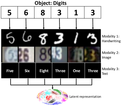
Figure 1: A graphical framework for multimodal learning in which we have access to 3 data modalities: handwriting, images, and text, describing the same object, a digit. Multimodal learning models relate these sources of information to learn a data representation that embeds information on all data modalities.

Multimodal learning is the field in machine learning that designs models which can process and relate information from different stimuli or data modalities (Baltrušaitis et al., 2018). There are two main approaches for multimodal representation learning: i) joint representation and ii) coordinated representation. The former uses all modalities as inputs and projects them into a common space, while the latter assumes that each representation exists in its own space and all representations are coordinated through a similarity or structure constraint (Baltrušaitis et al., 2018). However, it is common to use the term “joint representations” to refer to data representations that embed information from multiple data modalities, regardless of the learning approach. Figure 1 (Mancisidor et al., 2021) shows a multimodal learning scheme, in which we have access to three different modalities (handwriting, image, and text) representing a common object (digits). A multimodal learning model learns a data representation that embeds useful information from each data modality.

In this research, we use the CMMD model, which uses the joint representation approach for representation learning and at the same time trains a classifier conditioned on the learned latent representations. In addition, as we explain in Section 3.3, the CMMD model optimizes mutual information between missing modalities and latent representations used for classification, achieving a more accurate classification.

3.2 Variational Inference

The objective function optimized by the CMMD model is obtained by using the Variational Inference (VI) approach. Therefore, in what follows, we provide a short description of this method. Assume that we have access to $N$ observations and latent variables, i.e., $\bm{X}=\{{\bm{x}}_{1},{\bm{x}}_{2},\cdots,{\bm{x}}_{N}\}$ and $\bm{Z}=\{{\bm{z}}_{1},{\bm{z}}_{2},\cdots,{\bm{z}}_{N}\}$, that are related through the joint density $p(\bm{Z},\bm{X})=p(\bm{X}|\bm{Z})P(\bm{Z})$. Assuming a full factorization for $p(\bm{Z})=\prod_{n=1}^{N}p({\bm{z}}_{i})$ and $p(\bm{X}|\bm{Z})=\prod_{n=1}^{N}p({\bm{x}}_{i}|{\bm{z}}_{i})$, the average marginal log-likelihood of the data set $\bm{X}$ is simply $\frac{1}{N}\log p(\bm{X})=\frac{1}{N}\sum_{i=1}^{N}\log p({\bm{x}}_{i})$. The marginal log-likelihood is, however, intractable due to the integral $\int p(\bm{X},\bm{Z})d\bm{Z}$ (Kingma and Welling, 2013; Blei et al., 2017). VI circumvents this problem by noting that the marginal log-likelihood for the ith observation can be written as

$$\log p({\bm{x}}^{i})= \log\int p({\bm{x}}^{i},{\bm{z}})d{\bm{z}}$$

$$= \log\int q({\bm{z}}|{\bm{x}}^{i})\frac{p({\bm{x}}^{i}|{\bm{z}})p({\bm{z}})}{q({\bm{z}}|{\bm{x}}^{i})}d{\bm{z}}$$

$$= \log\mathbb{E}_{q({\bm{z}}|{\bm{x}}^{i})}\frac{p({\bm{x}}^{i}|{\bm{z}})p({\bm{z}})}{q({\bm{z}}|{\bm{x}}^{i})}$$

$$\geq \mathbb{E}_{q({\bm{z}}|{\bm{x}}^{i})}[\log p({\bm{x}}^{i}|{\bm{z}})+\log p({\bm{z}})-\log q({\bm{z}}|{\bm{x}}^{i})]$$

$$\equiv$$ ELBO (1)

where $q({\bm{z}}|{\bm{x}})$ is a variational distribution (also called inference or recognition model) approximating the true posterior distribution $p({\bm{z}}|{\bm{x}})$, and the inequality is a result of the concavity of log and Jensen’s inequality. Hence, VI optimizes intractable problems by introducing variational distributions and maximizing the Evidence Lower Bound (ELBO) in Equation 1, instead of the intractable marginal log-likelihood. Note that the ELBO in Equation 1 can be derived by minimizing the divergence $KL[q({\bm{z}}|{\bm{x}})||p({\bm{z}}|{\bm{x}})]$ and, in that case, the ELBO can be rewritten as $\text{ELBO}=\log p({\bm{x}}^{i})-KL[q({\bm{z}}|{\bm{x}}^{i})||p({\bm{z}}|{\bm{x}}^{i})]$. Therefore, maximizing the ELBO is equivalent to minimizing the Kullbak-Leibler divergence between the true posterior and its variational approximation, which turns out to improve the tightness of the lower bound.

3.2.1 Variational Inference with Deep Neural Networks

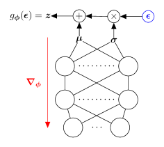
Figure 2: Architecture of a neural network that learns the parameters $\bm{\mu}$ and $\bm{\sigma}$ of a Gaussian distribution. The output layer $\bm{\mu}$ has the same number of neurons as the dimensionality of ${\bm{z}}$. Then we draw a representation ${\bm{z}}$ by using the location-scale transformation ${\bm{z}}=\bm{\mu}+\bm{\sigma}\odot\bm{\epsilon}$, where $\bm{\epsilon}\sim\mathcal{N}(\bm{0},\bm{1})$ and $\odot$ is the element-wise product.

Kingma and Welling (2013) and Rezende et al. (2014) coupled VI methods with deep neural networks and show how these models can be efficiently optimized by backpropagation and the AutoEncoding Variational Bayesian (AEVB) algorithm (Kingma and Welling, 2013). Assume that both densities $q({\bm{z}}|{\bm{x}})$ and $p({\bm{x}}|{\bm{z}})$ in Equation 1 follow a Gaussian distribution with diagonal covariance matrix, and that $p({\bm{z}})$ is an isotropic Gaussian distribution, where ${\bm{z}}\in\mathbb{R}^{d}$. The ELBO in Equation 1 then takes the form

$$\text{ELBO}= \log p_{\bm{\theta}}({\bm{x}}|{\bm{z}})-KL[q_{\bm{\phi}}({\bm{z}}|{\bm{x}})||p({\bm{z}})]$$

$$= \log\mathcal{N}({\bm{x}}|{\bm{z}};\bm{\mu}=f_{\theta}({\bm{z}}),\bm{\sigma}^{2}=f_{\theta}({\bm{z}}))-KL[\mathcal{N}({\bm{z}}|{\bm{x}};\bm{\mu}=f_{\phi}({\bm{x}}),\bm{\sigma}^{2}=f_{\phi}({\bm{x}}))||\mathcal{N}({\bm{z}};\bm{0},\bm{1})]$$

$$= \log\mathcal{N}({\bm{x}}|{\bm{z}};\bm{\mu}=f_{\theta}({\bm{z}}),\bm{\sigma}^{2}=f_{\theta}({\bm{z}}))+\frac{1}{2}\sum_{j=1}^{d}(1+\log\sigma_{j}^{2}-\mu_{j}^{2}-\sigma_{j}^{2}),$$

where $f(\cdot)$ denotes a function composed by a neural network with trainable parameters $\bm{\theta}$ and $\bm{\phi}$ for the generative and inference model, respectively, and $d$ is the dimension of ${\bm{z}}$. Given that the variational distribution and the prior density are both Gaussian, the Kullback-Leibler divergence has a closed-form. Figure 2 shows the architecture of a neural network for the inference model $q({\bm{z}}|{\bm{x}})$. Note that the output layer of such a neural network contains the Gaussian parameters, and that ${\bm{z}}$ is drawn using the location-scale transformation ${\bm{z}}=\bm{\mu}+\bm{\sigma}\odot\bm{\epsilon}$ where $\bm{\epsilon}\sim\mathcal{N}(\bm{0},\bm{1})$ and $\odot$ is the element-wise product. Such an architecture has the advantage that it can be backpropagated. This implies that by updating the trainable parameters $\bm{\theta}$ and $\bm{\phi}$ of the neural network, we learn the parameters $\bm{\mu}$ and $\bm{\sigma}$ for the inference and generative model, respectively, that maximize the ELBO.

At this point, it is worth mentioning that the inference model $q({\bm{z}}|{\bm{x}})$ generates a code of the input data and the generative model $p({\bm{x}}|{\bm{z}})$ takes that code and generates a new instance of the input data. Hence, $q({\bm{z}}|{\bm{x}})$ is often referred to as a probabilistic encoder and $p({\bm{x}}|{\bm{z}})$ is referred to as a probabilistic decoder. Further, note that the code ${\bm{z}}$ is just a representation in a latent space for the input data ${\bm{x}}$. Therefore, it is common to call ${\bm{z}}$ a data representation or simply a representation in short.

3.3 Conditional MultiModal Discriminative Model (CMMD)

The CMMD model relates information from multiple data modalities, assuming that we have access to all modalities and class labels only for model training. That is, at training time we observe $(\bm{x}_{\scriptstyle\scriptscriptstyle\mathcal{O}},\bm{x}_{\scriptstyle\scriptscriptstyle\mathcal{M}},y)$, where $\bm{x}_{\scriptstyle\scriptscriptstyle\mathcal{O}}=({\bm{x}}_{1},\cdots,{\bm{x}}_{n})$ are n modalities that are always observed, and $\bm{x}_{\scriptstyle\scriptscriptstyle\mathcal{M}}=({\bm{x}}_{n+1},\cdots,{\bm{x}}_{n+m})$ are m modalities that together with class labels $y$ are missing at test time. Hence, only $\bm{x}_{\scriptstyle\scriptscriptstyle\mathcal{O}}$ is available during both training and test time. At test time, the CMMD model generates multimodal representations ${\bm{z}}$ using a prior distribution $p({\bm{z}}|\bm{x}_{\scriptstyle\scriptscriptstyle\mathcal{O}})$ conditioned on the observed modalities. These representations ${\bm{z}}\sim p({\bm{z}}|\bm{x}_{\scriptstyle\scriptscriptstyle\mathcal{O}})$ are used in both the generative process $p(\bm{x}_{\scriptstyle\scriptscriptstyle\mathcal{M}}|\bm{x}_{\scriptstyle\scriptscriptstyle\mathcal{O}},{\bm{z}})$ and in the classifier model $p(y|{\bm{z}})$. This learning process encourages the CMMD model to learn multimodal representations that are useful for classification and generating the missing modalities at test time.

The generative model in CMMD factorizes as $p(\bm{x}_{\scriptstyle\scriptscriptstyle\mathcal{M}},y,{\bm{z}}|\bm{x}_{\scriptstyle\scriptscriptstyle\mathcal{O}})=p(y|{\bm{z}})p({\bm{z}}|\bm{x}_{\scriptstyle\scriptscriptstyle\mathcal{O}})p(\bm{x}_{\scriptstyle\scriptscriptstyle\mathcal{M}}|\bm{x}_{\scriptstyle\scriptscriptstyle\mathcal{O}},{\bm{z}})$ and, under this model specification, the posterior distribution $p({\bm{z}}|\bm{x}_{\scriptstyle\scriptscriptstyle\mathcal{O}},\bm{x}_{\scriptstyle\scriptscriptstyle\mathcal{M}},y)$ is intractable (Mancisidor et al., 2021). Therefore, CMMD uses VI and approximates the true posterior distribution with a variational density $q({\bm{z}}|\bm{x}_{\scriptstyle\scriptscriptstyle\mathcal{O}},\bm{x}_{\scriptstyle\scriptscriptstyle\mathcal{M}},y)$. Hence, the variational lower bound on the marginal log-likelihood of the data is

$$\log p(\bm{x}_{\scriptstyle\scriptscriptstyle\mathcal{M}},y|\bm{x}_{\scriptstyle\scriptscriptstyle\mathcal{O}})= \log\int p(\bm{x}_{\scriptstyle\scriptscriptstyle\mathcal{M}},y,{\bm{z}}|\bm{x}_{\scriptstyle\scriptscriptstyle\mathcal{O}})d{\bm{z}}$$

$$= \log\int q({\bm{z}}|\bm{x}_{\scriptstyle\scriptscriptstyle\mathcal{O}},\bm{x}_{\scriptstyle\scriptscriptstyle\mathcal{M}},y)\frac{p(\bm{x}_{\scriptstyle\scriptscriptstyle\mathcal{M}},y,{\bm{z}}|\bm{x}_{\scriptstyle\scriptscriptstyle\mathcal{O}})}{q({\bm{z}}|\bm{x}_{\scriptstyle\scriptscriptstyle\mathcal{O}},\bm{x}_{\scriptstyle\scriptscriptstyle\mathcal{M}},y)}d{\bm{z}}$$

$$= \log\mathbb{E}_{q({\bm{z}}|\bm{x}_{\scriptstyle\scriptscriptstyle\mathcal{O}},\bm{x}_{\scriptstyle\scriptscriptstyle\mathcal{M}},y)}\frac{p(\bm{x}_{\scriptstyle\scriptscriptstyle\mathcal{M}},y,{\bm{z}}|\bm{x}_{\scriptstyle\scriptscriptstyle\mathcal{O}})}{q({\bm{z}}|\bm{x}_{\scriptstyle\scriptscriptstyle\mathcal{O}},\bm{x}_{\scriptstyle\scriptscriptstyle\mathcal{M}},y)}$$

$$\geq \mathbb{E}_{q({\bm{z}}|\bm{x}_{\scriptstyle\scriptscriptstyle\mathcal{O}},\bm{x}_{\scriptstyle\scriptscriptstyle\mathcal{M}},y)}\bigg{[}\log\frac{p(\bm{x}_{\scriptstyle\scriptscriptstyle\mathcal{M}},y,{\bm{z}}|\bm{x}_{\scriptstyle\scriptscriptstyle\mathcal{O}})}{q({\bm{z}}|\bm{x}_{\scriptstyle\scriptscriptstyle\mathcal{O}},\bm{x}_{\scriptstyle\scriptscriptstyle\mathcal{M}},y)}\bigg{]}$$

$$= \mathbb{E}_{q({\bm{z}}|\bm{x}_{\scriptstyle\scriptscriptstyle\mathcal{O}},\bm{x}_{\scriptstyle\scriptscriptstyle\mathcal{M}},y)}[\log p(\bm{x}_{\scriptstyle\scriptscriptstyle\mathcal{M}}|\bm{x}_{\scriptstyle\scriptscriptstyle\mathcal{O}},{\bm{z}})+\log p(y|{\bm{z}})+\log p({\bm{z}}|\bm{x}_{\scriptstyle\scriptscriptstyle\mathcal{O}})-\log q({\bm{z}}|\bm{x}_{\scriptstyle\scriptscriptstyle\mathcal{O}},\bm{x}_{\scriptstyle\scriptscriptstyle\mathcal{M}},y)]$$

$$= \mathbb{E}_{q({\bm{z}}|\bm{x}_{\scriptstyle\scriptscriptstyle\mathcal{O}},\bm{x}_{\scriptstyle\scriptscriptstyle\mathcal{M}},y)}[\log p(\bm{x}_{\scriptstyle\scriptscriptstyle\mathcal{M}}|\bm{x}_{\scriptstyle\scriptscriptstyle\mathcal{O}},{\bm{z}})+\log p(y|{\bm{z}})]-KL[q({\bm{z}}|\bm{x}_{\scriptstyle\scriptscriptstyle\mathcal{O}},\bm{x}_{\scriptstyle\scriptscriptstyle\mathcal{M}},y)||\log p({\bm{z}}|\bm{x}_{\scriptstyle\scriptscriptstyle\mathcal{O}})],$$ (2)

where the inequality is a result of the concavity of log and Jensen’s inequality. Equation 3.3 contains an upper bound on the mutual information between $\bm{x}_{\scriptstyle\scriptscriptstyle\mathcal{M}}$ and ${\bm{z}}$ (Mancisidor et al., 2021), which is exactly a property that we want to maximize. That is, we are interested in learning representations ${\bm{z}}$ that embed as much information as possible about the missing modalities $\bm{x}_{\scriptstyle\scriptscriptstyle\mathcal{M}}$. To achieve this, the CMMD model includes a conditional mutual information $I(\bm{x}_{\scriptstyle\scriptscriptstyle\mathcal{M}},{\bm{z}}|\bm{x}_{\scriptstyle\scriptscriptstyle\mathcal{O}})$ into the lower bound in Equation 3.3 to obtain the following likelihood-free objective function

$$\mathcal{J}(\bm{x}_{\scriptstyle\scriptscriptstyle\mathcal{O}},\bm{x}_{\scriptstyle\scriptscriptstyle\mathcal{M}},y)= \mathbb{E}_{q({\bm{z}}|\bm{x}_{\scriptstyle\scriptscriptstyle\mathcal{O}},\bm{x}_{\scriptstyle\scriptscriptstyle\mathcal{M}},y)}[\log p(\bm{x}_{\scriptstyle\scriptscriptstyle\mathcal{M}}|\bm{x}_{\scriptstyle\scriptscriptstyle\mathcal{O}},{\bm{z}})+\log p(y|{\bm{z}})]$$

$$- KL[q({\bm{z}}|\bm{x}_{\scriptstyle\scriptscriptstyle\mathcal{O}},\bm{x}_{\scriptstyle\scriptscriptstyle\mathcal{M}},y)||\log p({\bm{z}}|\bm{x}_{\scriptstyle\scriptscriptstyle\mathcal{O}})]+(1-\omega)I(\bm{x}_{\scriptstyle\scriptscriptstyle\mathcal{M}},{\bm{z}}|\bm{x}_{\scriptstyle\scriptscriptstyle\mathcal{O}})$$

$$= \mathbb{E}_{q({\bm{z}}|\bm{x}_{\scriptstyle\scriptscriptstyle\mathcal{O}},\bm{x}_{\scriptstyle\scriptscriptstyle\mathcal{M}},y)}[\log p(\bm{x}_{\scriptstyle\scriptscriptstyle\mathcal{M}}|\bm{x}_{\scriptstyle\scriptscriptstyle\mathcal{O}},{\bm{z}})+\log p(y|{\bm{z}})]$$

$$- \omega KL[q({\bm{z}}|\bm{x}_{\scriptstyle\scriptscriptstyle\mathcal{O}},\bm{x}_{\scriptstyle\scriptscriptstyle\mathcal{M}},y)||p({\bm{z}}|\bm{x}_{\scriptstyle\scriptscriptstyle\mathcal{O}})]-(1-\omega)KL[q({\bm{z}}|\bm{x}_{\scriptstyle\scriptscriptstyle\mathcal{O}})||p({\bm{z}}|\bm{x}_{\scriptstyle\scriptscriptstyle\mathcal{O}})],$$ (3)

where $\omega\in[0,1]$ is a weight hyperparameter controlling the influence of the mutual information term. Note that for $\omega=1$, Equation 3 recovers the evidence lower bound in Equation 3.3. The density functions in the CMMD model are assumed to be

$$p(\bm{x}_{\scriptstyle\scriptscriptstyle\mathcal{M}}|\bm{x}_{\scriptstyle\scriptscriptstyle\mathcal{O}},{\bm{z}})\sim \mathcal{N}(\bm{x}_{\scriptstyle\scriptscriptstyle\mathcal{M}}|\bm{x}_{\scriptstyle\scriptscriptstyle\mathcal{O}},{\bm{z}};\bm{\mu}=f_{\bm{\theta}}(\bm{x}_{\scriptstyle\scriptscriptstyle\mathcal{O}},{\bm{z}}),\bm{\sigma}^{2}=f_{\bm{\theta}}(\bm{x}_{\scriptstyle\scriptscriptstyle\mathcal{O}},{\bm{z}}))$$

$$p({\bm{z}}|\bm{x}_{\scriptstyle\scriptscriptstyle\mathcal{O}})\sim \mathcal{N}({\bm{z}}|\bm{x}_{\scriptstyle\scriptscriptstyle\mathcal{O}};\bm{\mu}=f_{\bm{\theta}}(\bm{x}_{\scriptstyle\scriptscriptstyle\mathcal{O}}),\bm{\sigma}^{2}=f_{\bm{\theta}}(\bm{x}_{\scriptstyle\scriptscriptstyle\mathcal{O}}))$$

$$q({\bm{z}}|\bm{x}_{\scriptstyle\scriptscriptstyle\mathcal{O}},\bm{x}_{\scriptstyle\scriptscriptstyle\mathcal{M}},y)\sim \mathcal{N}({\bm{z}}|\bm{x}_{\scriptstyle\scriptscriptstyle\mathcal{O}},\bm{x}_{\scriptstyle\scriptscriptstyle\mathcal{M}},y;\bm{\mu}=f_{\bm{\phi}}(\bm{x}_{\scriptstyle\scriptscriptstyle\mathcal{O}},\bm{x}_{\scriptstyle\scriptscriptstyle\mathcal{M}},y),\bm{\sigma}^{2}=f_{\bm{\phi}}(\bm{x}_{\scriptstyle\scriptscriptstyle\mathcal{O}},\bm{x}_{\scriptstyle\scriptscriptstyle\mathcal{M}},y))$$

$$p(y|{\bm{z}})\sim \text{Bernoulli}(y|{\bm{z}};\pi=f_{\bm{\theta}}({\bm{z}})),$$ (4)

where Gaussian distributions $\mathcal{N}(\cdot)$ assume a diagonal covariance matrix, $f(\cdot)$ denotes a multilayer perceptron model that learns density parameters, $\bm{\theta}$ and $\bm{\phi}$ denote all trainable neural network weights for the generative and inference model, respectively, and ($\bm{\mu}$, $\bm{\sigma}^{2}$) and $\pi$ are the density parameters for the Gaussian and Bernoulli distributions. Figure 3 (Mancisidor et al., 2021) shows the architecture for the CMMD model, which contains a posterior and a prior distribution for multimodal representations, a generative model for missing modalities, and a classifier for class labels.

It is noteworthy that minimizing the divergence term $KL[q({\bm{z}}|\bm{x}_{\scriptstyle\scriptscriptstyle\mathcal{O}},\bm{x}_{\scriptstyle\scriptscriptstyle\mathcal{M}},y)||p({\bm{z}}|\bm{x}_{\scriptstyle\scriptscriptstyle\mathcal{O}})]$ in Equation 3 has the effect of bringing the prior close to the posterior (Suzuki et al., 2016) and it also minimizes the expected information required to convert a sample from the prior into a sample from the posterior distribution (Doersch, 2016). This effect is critical to learn multimodal representations that embed information from all data modalities.

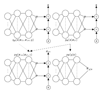
Figure 3: Architecture for the CMMD model that is composed by 4 neural networks: encoder, decoder, prior, and classifier. The dotted arrow indicates a forward pass during training, which is replaced by the dashed arrow at test time, i.e., the input to $p(\bm{x}_{\scriptstyle\scriptscriptstyle\mathcal{M}}|\bm{x}_{\scriptstyle\scriptscriptstyle\mathcal{O}},{\bm{z}})$ is ${\bm{z}}\sim q({\bm{z}}|\bm{x}_{\scriptstyle\scriptscriptstyle\mathcal{O}},\bm{x}_{\scriptstyle\scriptscriptstyle\mathcal{M}},y)$ during training, while ${\bm{z}}\sim p({\bm{z}}|\bm{x}_{\scriptstyle\scriptscriptstyle\mathcal{O}})$ at test time. The solid arrow depicts a common forward propagation during training and testing, i.e., the input to $p(y|{\bm{z}})$ is always ${\bm{z}}\sim p({\bm{z}}|\bm{x}_{\scriptstyle\scriptscriptstyle\mathcal{O}})$.

3.3.1 CMMD for Corporate Bankruptcy Prediction

In the context of corporate bankruptcy prediction, the modalities that are always observed are $\bm{x}_{\scriptstyle\scriptscriptstyle\mathcal{O}}=({\bm{x}}_{1},{\bm{x}}_{2})$, representing accounting and market information, since this information can easily be obtained for all companies on quarterly and daily basis, respectively. On the other hand, $\bm{x}_{\scriptstyle\scriptscriptstyle\mathcal{M}}={\bm{x}}_{3}$ and $y$ correspond to the MDA section in Form 10-K and class labels, respectively, which are assumed to be missing at test time. It makes sense to treat the MDA section as a modality that is not always observable, due to the fact that we rely on technical procedures to extract it from Form 10-K. In addition, not all public companies are under obligation to file annual reports containing such a section. Furthermore, in a real forecast scenario we do not have access to class labels and therefore they cannot be treated as an always observable modality.

The CMMD model uses accounting and market modalities to define an informative prior distribution, which generates data representations. When the MDA is available during model training, the CMMD model draws data representations from a posterior distribution that is updated by this data modality. Furthermore, class posterior probabilities $\pi$ in the CMMD classifier are estimated based on data representations, i.e., $p(y|{\bm{z}})$ with ${\bm{z}}\sim p({\bm{z}}|\bm{x}_{\scriptstyle\scriptscriptstyle\mathcal{O}})$. This classification approach differs from the traditional method where posterior probabilities $\pi^{\prime}$ are estimated based on observed features, i.e., $p(y|\bm{x}_{\scriptstyle\scriptscriptstyle\mathcal{O}})$. Through an efficient learning mechanism, the CMMD model aligns the parameters in the prior and posterior distributions. Therefore, the CMMD classifier anchors its forecasts on data representations that, despite being drawn by the prior distribution, contain information from all data modalities.

To make this point clear, let $q(y|\bm{x}_{\scriptstyle\scriptscriptstyle\mathcal{O}})\sim\text{Bernoulli}(\pi^{\prime})$ be a classifier model that estimates posterior class probabilities $\pi^{\prime}$ given $\bm{x}_{\scriptstyle\scriptscriptstyle\mathcal{O}}$, and the let the CMMD classifier be specified as in Equation 4. Further, let $\bm{Z}_{{\bm{X}_{\scriptstyle\scriptscriptstyle\mathcal{O}}}_{te}}$ denote a data set of representations drawn from the CMMD prior distribution $p({\bm{z}}|\bm{x}_{\scriptstyle\scriptscriptstyle\mathcal{O}})$, where ${\bm{X}_{\scriptstyle\scriptscriptstyle\mathcal{O}}}_{te}$ is a test data set composed by the observable modalities $\bm{x}_{\scriptstyle\scriptscriptstyle\mathcal{O}}$. Given that the CMMD model estimates class posterior probabilities based on representations that embed information from all data modalities, the classification performance of posterior probabilities $\pi_{i}$ for all $i$ in $\bm{Z}_{{\bm{X}_{\scriptstyle\scriptscriptstyle\mathcal{O}}}_{te}}$, should be relatively higher than that of posterior probabilities $\pi^{\prime}_{j}$ for all $j$ in ${\bm{X}_{\scriptstyle\scriptscriptstyle\mathcal{O}}}_{te}$.

4 Data

The data used in this research represent the largest data set ever used for bankruptcy prediction (Table 1). The data set includes accounting, market, and MDA data for publicly traded firms in NYSE, NASDAQ, and AMEX stock exchanges in the period 1994-2020. Accounting and market data are extracted from Wharton Research Data Services (WRDS), which provides access to Compustat Fundamentals and to the Center for Research in Security Prices (CRSP). The MDA section is directly extracted from the Form 10-K, which is available at the Electronic Data, Gathering, Analysis, and Retrieval (EDGAR) system provided by the U.S. Securities and Exchange Commission (SEC). The bankruptcy data used in this research are an updated version of the data used in Chava (2014), which are a comprehensive sample including the majority of publicly listed firms that filed for either Chapter 7 or 11 in the period 1964-2020.

Our data set is constructed in a similar way as in Shumway (2001) and Mai et al. (2019), i.e., letting each firm-quarter represents a separate observation. Hence, for each quarter we collect 31 accounting and 2 market predictors (Table 2). These 33 predictors are merged with the MDA corresponding to the same quarter. To construct a quarterly panel data, we roll-over the MDA data for 3 more quarters merging it with the corresponding predictors in the following 3 quarters. Hence, the same MDA is used for 4 quarters (Figure 4 panel (a)). After 4 quarters, we should get a new MDA that can be merged with its corresponding 33 predictors. If that is not the case, all firm-quarter observations will be missing until we get a new MDA. Finally, to make sure that all information is available for forecasting, we lag all observations by one period.

In this research, we predict bankruptcy for three different forecast horizons: 1, 2, and 3 years (Figure 4 panel (b)). Therefore, the set of 33 predictors and MDA are merged with 1, 2, and 3 years-ahead bankruptcies (Figure 4 panel (a)). For simplicity, we remove all firms from our data set after they file either for Chapter 7 or 11, i.e., the data set does not include reorganized firms after Chapter 11 was filed. Bankruptcies for which we cannot merge a set of predictors, regardless of the forecasting horizons, are discarded from our data set. After merging accounting, market, and MDA data, our data set for 1-year predictions contains 181,472 observations for model training, of which 699 are bankruptcies, and 40,950 observations for testing the model performance, of which 110 are bankruptcies. For 2-years predictions, the training data has 179,181 observations, of which 668 are bankruptcies, and the test data has 27,369 observations with 84 bankruptcies. Finally, the data set for 3-year predictions has 177,835 observations for model training, containing 588 bankruptcies, and 13,725 observations for testing the model, of which 54 are bankruptcies. Figure 5 shows the number of yearly bankruptcies and bankruptcy rates in our data set for 1-year bankruptcy predictions. Note that bankruptcy rates include only firm-quarter observations for which we could either merge the 3 data modalities (healthy firms) or the 3 data modalities with the bankruptcy data (bankrupted firms). On the other hand, the number of bankruptcies represents all yearly bankrupted firms in our bankruptcy data. This difference explains the discrepancy between bankruptcy rate and number of bankruptcies in 2012, as shown in Figure 5.

Table 2: Accounting and market variables used for bankruptcy prediction. The first column shows the variable names, while the second column shows their corresponding column names in the WRDS data base. All accounting information is extracted from comp.fundq and market information from crsp.msf and crsp.dsf. In the column Variable, we use the following abbreviations: ME_TL is market equity + total liabilities, TE is total equity and is calculated as the equity sum for all companies in a given quarter, C&SI is Cash and Short-term Investment, RE is Retained Earnings, CL is Current Liabilities

Variable	Database Names	Variable	Database Names
Assets/Liabilities	actq/lctq	Market-to-Book Ratio	(cshoq*prccq)/(atq-ltq)
Accounts payable/Sales	apq/saleq	Net Income/Total Assets	niq/atq
C&SI/Total Assets	cheq/atq	Net Income/ME_TL	niq/(cshoq*prccq+ltq)
C&SI/ME_TL	cheq/(cshoq*prccq+ltq)	Net Income/Sales	niq/saleq
Cash/Total Assets	chq/atq	Operating Income/Total Asset	oiadpq/atq
Cash/CL	chq/lctq	Operating Income/Sales	oiadpq/saleq
Total Debts/Total Assets	(dlcq+0.5*dlttq)/atq	Quick Assets/CL	(actq-invtq)/lctq
Growth of Inventories /Inventories	invchy/saley	RE/Total Asset	req/atq
Inventories/Sales	invtq/saleq	RE/CL	req/lctq
(CL – Cash)/Total Asset	(lctq-chq)/atq	Sales/Total Assets	saleq/atq
CL/Total Asset	lctq/atq	Equity/Total Asset	seqq/atq
CL/Total Liabilities	lctq/ltq	Working Capital/Total Assets	wcapq/atq
CL/Sales	lctq/saleq	Rsize	log(cshoq*prccq)/TE
Total Liabilities/Total Assets	ltq/atq	Log Price	log(min(prccq,15))
Total Liabilities/ME_TL	ltq/(cshoq*prccq+ltq)	Excess Return Over S&P 500	ret - vwretd
Log(Total Assets)	log(atq)	Stock Volatility	std(ret)
Log(Sale)	log(abs(saleq))

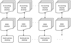
(a)

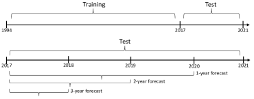
(b)

Figure 4: (a): We collect 31 accounting and 2 market predictors that are merged with an MDA from the same quarter. We roll-over the MDA data for 3 more quarters and merge it with the corresponding predictors in those 3 quarters, i.e., an MDA can be used during 4 quarters. (b): The data set in this research includes bankruptcies from 1994 to 2020. We use data from 1994 to 2016 for model training, while data from 2017 to 2020 are used for testing the predictive power of the models. For 1-year forecasts, for example, the latest quarter in which we can make a forecast is 2019Q4, which corresponds to bankruptcies during 2020Q4.

4.1 Data preprocessing

MDA sections are extracted from the company’s annual reports in Form 10-K and are transformed into a clean text file. Then, we follow the basic steps in natural language processing, i.e., word tokenization, remove stopwords, and stemming. We observe that some MDA documents do not contain substantial information, hence we include MDA documents containing more than 1,500 word tokens. This ensures that MDA documents contain substantial information. We use Term Frequency-Inverse Document Frequency (TF-IDF) to convert the preprocessed MDA documents into a numerical representation with 20,000 dimensions. This is the same number of dimensions as in Mai et al. (2019).

We use similar accounting ratios as in previous research, e.g., Altman (1968); Beaver (1966) and Mai et al. (2019), which reflect the liability, liquidity, and profitability for each company. The main difference with our data set is, however, that we construct a panel data with quarterly observations as shown in Figure 4 panel (a). By doing that, our data set is significantly larger than previous data sets, which is needed to train a model like CMMD. The data set used in Mai et al. (2019), for example, contains only 99,994 firm-year observations compared to 181,472 firm-quarter observations in our data set. All accounting variables are extracted from the Compustat table comp.funq and their calculation is shown in Table 2. In addition, excess returns, defined as the stock return relative to the S&P 500 returns, and stock volatility, defined as the standard deviation for stock returns in the past 63 days, are extracted from CRSP tables crsp.msf and crsp.dsf. Finally, accounting and market variables are scaled in the range 0 and 1 to match the scale of TF-IDF vectors.

Given that the class labels in the data set are highly imbalanced, we down-sample the majority class ($y=0$) until it equals the number of observations in the minority class ($y=1$) for model training. On the other hand, the test data set preserves its original number of classes, ensuring that models are tested on real scenarios.

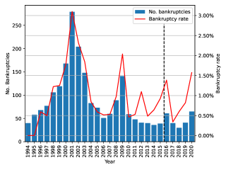
Figure 5: Number of yearly bankruptcies and bankruptcy rates in our data set for 1-year bankruptcy predictions. Bankruptcy rate includes firm-quarter observations for which we could either merge the 3 data modalities or merge the 3 data modalities with 1-year ahead bankruptcies, while the number of bankruptcies include all listed companies that file for Chapter 7 or 11.

5 Experiments and Results

This section compares our proposed methodology for bankruptcy prediction, which is based on multimodal representations generated by the CMMD model, with the traditional approach in which the classifier model is trained and tested on the same observed predictors. To that end, we include the following benchmark models: Logistic Regression (LR), Support Vector Machine (SVM), Multilayer Perceptron (MLP), k-Nearest Neighbors (k-NN), Random Forests (RF), and Naive Bayes (NB). We measure the classification performance of all models using different indicators that evaluate performance from different perspectives. Specifically, we use the Area Under the ROC Curve (AUC) and H-measure (Hand, 2009) as global performance metrics, and the Kolmogorov-Smirnov (KS) test as a local performance metric. Note that all three metrics estimate classification performance in the interval [0 1]. Finally, Section 5.3 analyzes the information embedded in the multimodal representations ${\bm{z}}\sim p({\bm{z}}|\bm{x}_{\scriptstyle\scriptscriptstyle\mathcal{O}})$.

The CMMD model is implemented in TensorFlow and it is trained using the Adam optimizer (Kingma and Ba, 2014) with default values. To provide a fair model comparison, we fine-tune the hyperparameters for all models for all forecast horizons. Appendix 8 shows the grid-search values in our fine-tuning approach, as well as the final architecture for each model and each forecast horizon.

5.1 Experimental Design

We conduct three different experiments to compare the classification performance of our proposed methodology with that of all benchmark models. In Experiments I and II we use the time period 1994 - 2007 for training and the time period 2008 - 2014 for testing, while in Experiment III we use the time period 1994 - 2016 for training and the time period 2017 - 2020 for testing. The difference between Experiment I and Experiment II is that the former uses training and test sets consisting of $\bm{x}_{\scriptstyle\scriptscriptstyle\mathcal{O}}$ only for the benchmark models, while in the latter we also use ${\bm{x}}_{3}$, the 20,000 TF-IDF variables. In both experiments, the CMMD model uses all three modalities for training, and only the accounting and market data for testing.

The time period used in Experiments I and II is chosen to provide a fair and direct comparison with the DL-Embedding + DL-1 Layer model introduced in Mai et al. (2019). Experiment III is similar to Experiment I, except for the fact that the training and test periods are different. These two experiments study the classical scenario in which multimodal learning models assess how much information from missing modalities has been embedded into the multimodal representation, see e.g., Shi et al. (2019); Wang et al. (2016); Sutter et al. (2021) or Mancisidor et al. (2021). Table 3 summarizes the data used in the three experiments. As can be seen from this table, the number of testing observations reduces from 89,582 in Experiment I to 36,240 in Experiment II. This is due to the fact that MDA information is not available for 37% of the test observations in Experiment I (the number of companies reduces from 5,203 to 3,132).

Table 3: Number of observations and bankruptcies, and bankruptcy rates during the two different time periods studied in this research. Experiments I and II are as explained in Section 5.1.

		From 1994 to 2014		From 1994 to 2020
		Experiment I	Experiment II	Experiment III
Training	Observations	122,916	122,916	181,472
	Bankruptcies	537	537	699
	Bankruptcy rate	0.4369%	0.4369%	0.3852%
Testing	Observations	89,582	36,240	40,950
	Bankruptcies	179	94	110
	Bankruptcy rate	0.1998%	0.2594%	0.2686%

5.2 Results

Experiments I and II:

Table 4 measures the classification performance, based on AUC, for 1 year bankruptcy predictions during the first time period from 1994 to 2014. In both Experiment I and II, RF is the model with highest AUC, followed by CMMD and SVM. Further, the benchmark models actually achieve higher classification performance in Experiment I than in Experiment II, meaning that the MDA data does not improve the prediction accuracy for these models. This is in agreement with Mai et al. (2019), where the only model with higher AUC when MDA is used is the one introduced by the authors. Note also that all methods except k-NN and NB achieve higher AUC values than the DL-Embedding model introduced in Mai et al. (2019). This suggests that using panel data based on firm-quarter observations gives more accurate bankruptcy predictions.

The CMMD-model is not able to beat the RF-model in these experiments. We believe that this is due to the fact that it requires more training data than the competing methods. Hence, in Experiment III we have repeated Experiment I for a longer training period.

Table 4: Model performance for 1-year bankruptcy predictions. We report average and standard deviation values for 5 different randomly selected training data sets during the period 1994 to 2007. The test period, in this case, is from 2008 to 2014. Results marked with ${\dagger}$ are taken from Mai et al. (2019).

Experiment I - ${\bm{x}}_{3}$ is missing at test time
Model Name	AUC	H-measure	KS
k-NN	0.8334 $\pm$ 0.0055	0.3633 $\pm$ 0.0122	0.5489 $\pm$ 0.0112
NB	0.6299 $\pm$ 0.0106	0.1719 $\pm$ 0.0084	0.2204 $\pm$ 0.0056
LR	0.8856 $\pm$ 0.0030	0.4643 $\pm$ 0.0040	0.6299 $\pm$ 0.0070
SVM	0.8868 $\pm$ 0.0037	0.4717 $\pm$ 0.0060	0.6289 $\pm$ 0.0123
RF	0.9234 $\pm$ 0.0024	0.5636 $\pm$ 0.0073	0.7302 $\pm$ 0.0055
MLP	0.8738 $\pm$ 0.0091	0.4797 $\pm$ 0.0172	0.6251 $\pm$ 0.0176
CMMD	0.8988 $\pm$ 0.0008	0.4847 $\pm$ 0.0020	0.6551 $\pm$ 0.0063
Experiment II - ${\bm{x}}_{3}$ is available at test time
k-NN	0.8253 $\pm$ 0.0233	0.3544 $\pm$ 0.0563	0.5358 $\pm$ 0.0427
NB	0.6113 $\pm$ 0.0465	0.1305 $\pm$ 0.0654	0.1799 $\pm$ 0.0699
LR	0.8888 $\pm$ 0.0038	0.4792 $\pm$ 0.0034	0.6389 $\pm$ 0.0057
SVM	0.8963 $\pm$ 0.0045	0.5159 $\pm$ 0.0061	0.6538 $\pm$ 0.0094
RF	0.9212 $\pm$ 0.0082	0.5675 $\pm$ 0.0275	0.7310 $\pm$ 0.0241
MLP	0.8773 $\pm$ 0.0052	0.4755 $\pm$ 0.0058	0.6241 $\pm$ 0.0103
CMMD	0.8913 $\pm$ 0.0003	0.5014 $\pm$ 0.0020	0.6576 $\pm$ 0.0107
DL-Embedding + DL-1 Layer	0.8420†

Experiment III:

Table 5 compares the classification performance for three different forecast horizons. We report the average performance, as well as the standard deviation of 5 different randomly selected training data sets. The test period is always the same and only varies depending on the forecast horizon.

Table 5: Model performance for 1-, 2-, and 3-year bankruptcy predictions. Experiment III: We report average and standard deviation values for 5 different randomly selected training data sets. The test period is always the same and it depends on the forecasting horizon. Training and test periods are shown in Figure 4 panel (b).

Model Name	AUC
	1 year	2 years	3 years
k-NN	0.8669 $\pm$ 0.0090	0.7809 $\pm$ 0.0088	0.7526 $\pm$ 0.0190
NB	0.8242 $\pm$ 0.0097	0.7328 $\pm$ 0.0085	0.7422 $\pm$ 0.0088
LR	0.8982 $\pm$ 0.0072	0.8229 $\pm$ 0.0061	0.8293 $\pm$ 0.0060
SVM	0.9017 $\pm$ 0.0057	0.8218 $\pm$ 0.0021	0.8167 $\pm$ 0.0023
RF	0.9251 $\pm$ 0.0047	0.8363 $\pm$ 0.0089	0.8404 $\pm$ 0.0092
MLP	0.9142 $\pm$ 0.0044	0.8355 $\pm$ 0.0083	0.8086 $\pm$ 0.0023
CMMD	$\bm{0.9315}$ $\pm$ 0.0011	$\bm{0.8581}$ $\pm$ 0.0031	$\bm{0.8473}$ $\pm$ 0.0060
	H-measure
k-NN	0.4602 $\pm$ 0.0355	0.2472 $\pm$ 0.0077	0.1968 $\pm$ 0.0457
NB	0.4116 $\pm$ 0.0292	0.2022 $\pm$ 0.0071	0.2162 $\pm$ 0.0124
LR	0.5710 $\pm$ 0.0057	0.3573 $\pm$ 0.0101	0.3486 $\pm$ 0.0159
SVM	0.5764 $\pm$ 0.0040	0.3278 $\pm$ 0.0110	0.3177 $\pm$ 0.0014
RF	0.5938 $\pm$ 0.0071	0.3424 $\pm$ 0.0174	0.3944 $\pm$ 0.0342
MLP	0.5875 $\pm$ 0.0108	0.3685 $\pm$ 0.0091	0.3085 $\pm$ 0.0208
CMMD	$\bm{0.6228}$ $\pm$ 0.0028	0.4058 $\pm$ 0.0043	0.3764 $\pm$ 0.0151
	KS
k-NN	0.6225 $\pm$ 0.0278	0.4463 $\pm$ 0.0227	0.3886 $\pm$ 0.0297
NB	0.6085 $\pm$ 0.0179	0.4252 $\pm$ 0.0105	0.4403 $\pm$ 0.0228
LR	0.7278 $\pm$ 0.0113	0.5619 $\pm$ 0.0067	0.5532 $\pm$ 0.0189
SVM	0.7229 $\pm$ 0.0067	0.5326 $\pm$ 0.0104	0.5516 $\pm$ 0.0027
RF	0.7371 $\pm$ 0.0063	0.5251 $\pm$ 0.0129	0.5604 $\pm$ 0.0334
MLP	0.7363 $\pm$ 0.0100	0.5565 $\pm$ 0.0058	0.5327 $\pm$ 0.0289
CMMD	$\bm{0.7695}$ $\pm$ 0.0039	0.5720 $\pm$ 0.0033	0.5880 $\pm$ 0.0178

As can be seen from the table, the CMMD model now achieves the highest AUC and KS values, which implies that the discriminative power of CMMD is higher than that of all benchmark models. All models perform better in this experiment than in Experiment I. However, for the RF-model the AUC-value is only slightly higher. Interestingly, the AUC and H-measure do not agree on the model with the most accurate 3-year predictions. For this particular forecast horizon, CMMD has the highest AUC value, while RF has the highest H-measure. The KS test suggests, however, that there is a threshold where the CMMD model achieves the largest separation of the two class labels. Hence, from this experiment, it is clear that if the training data set is sufficiently large, the CMMD model outperforms all benchmark models, suggesting that multimodal representations ${\bm{z}}$ embed information from all data modalities and stand out as the best predictor for corporate bankruptcy.

In Experiments I and III the CMMD model is used to compute predictions for all test observations. One might also consider a mixed approach in which the CMMD model is only used in the cases where the MDA data is missing and e.g. the RF model is used in the remaining cases.

5.3 Latent Representations of Companies

In order to better understand the multimodal representations ${\bm{z}}$, it is possible to visualize both the latent variables of the prior distribution ${\bm{z}}\sim p({\bm{z}}|\bm{x}_{\scriptstyle\scriptscriptstyle\mathcal{O}})$ and the time evolution of its parameters $\bm{\mu}$ and $\bm{\Sigma}$, which is a diagonal matrix with parameters $\bm{\sigma}$.

To visualize latent variables ${\bm{z}}$, we use the CMMD model from Experiment I to generate latent representations from the prior distribution $p({\bm{z}}|\bm{x}_{\scriptstyle\scriptscriptstyle\mathcal{O}})$ for the period 2017 to 2020. In this case, the dimension of the latent space is 50 (see Appendix 8), i.e. ${\bm{z}}\in\mathbb{R}^{50}$, hence we use t-SNE (Van der Maaten and Hinton, 2008) to obtain two-dimensional vectors that can be visualized.

Panel (a) in Figure 6 shows data representations for all companies during the entire test period, where the scatter color is given by the probability of bankruptcy estimated by the CMMD classifier. It is interesting to see that companies with relatively high probability of bankruptcy cluster in the upper-right corner. Further, panels (b) and (c) show representations during the first quarters of 2018 and 2019, respectively. Note that there are relatively fewer companies where the CMMD model estimates a high probability of bankruptcy during 2018Q1. From all figures, it is interesting to see that the estimated bankruptcy probability shows a smooth transition across the two-dimensional space. This suggests that the latent representations of the CMMD model are capable of capturing the spatial coherence (Bengio et al., 2013) of financial distress, which means that spatially near-by observations tend to be associated with the same value of probability of bankruptcy.

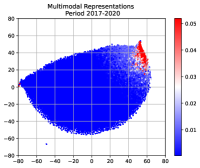
(a)

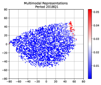
(b)

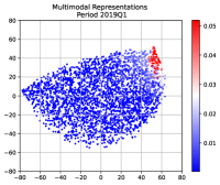
(c)

Figure 6: Latent representations for (a) the period 2017-2020, (b) the first quarter 2018, and (c) the first quarter 2019. The color of the scatter corresponds to the bankruptcy probability estimated by the CMMD model.

To follow the development over time of the parameters $\bm{\mu}$ and $\bm{\sigma}$, we aggregate quarterly latent variables ${\bm{z}}$ for all firms as follows: Let ${\bm{z}}^{k}\sim\mathcal{N}(\bm{\mu}^{k},\bm{\Sigma}^{k})$ be the latent representation for the the kth company. Given that all covariance terms are 0, the standard deviation (std) of the sum of all variables in ${\bm{z}}^{k}$ is $std(z_{1}^{k}+z_{2}^{k}+\cdots+z_{d}^{k})=\sqrt{\sum_{i=1}^{d}var(z_{i}^{k})}$, where $d$ is the dimension of ${\bm{z}}$. Therefore, we define an aggregated $\bm{\sigma}^{*}$ parameter for all companies as

$$\bm{\sigma}^{*}=\sum_{k=1}^{K}\sqrt{\sum_{i=1}^{d}var(z_{i}^{k})},$$ (5)

where $K$ is the total number of companies. Following the same logic, we define an aggregated $\bm{\mu}^{*}$ parameter for all companies as

$$\bm{\mu}^{*}=\sum_{k=1}^{K}\sum_{i=1}^{d}\mu_{i}^{k}.$$ (6)

For each quarter $q$ and company k, we generate multimodal representations ${\bm{z}}_{k}^{q}\sim p({\bm{z}}|\bm{x}_{\scriptstyle\scriptscriptstyle\mathcal{O}})$ and calculate yearly representations ${\bm{z}}_{k}^{Y}=\dfrac{1}{Q}\sum_{q=1}^{Q}{\bm{z}}_{k}^{q}$, where $Y$ denotes a given year and $Q$ is the latest observed quarter in $Y$. Finally, we calculate the aggregate yearly parameters $\bm{\sigma}_{Y}^{*}$ and $\bm{\mu}_{Y}^{*}$ using Equations 5 and 6.

We calculate $\bm{\mu}_{Y}^{*}$ and $\bm{\sigma}_{Y}^{*}$ for all years between 2008 to 2022 using a CMMD model trained with data from 1994 to 2007. Figure 7 compares the lagged parameters $\bm{\mu}^{*}$ and $\bm{\sigma}^{*}$ with the number of bankruptcies from 2008 to 2020. This comparison corresponds to the scenario of 1-year bankruptcy prediction, in which latent representations from the prior distribution ${\bm{z}}\sim p({\bm{z}}|\bm{x}_{\scriptstyle\scriptscriptstyle\mathcal{O}})$ during 2008 are used to forecast bankruptcies in 2009, for example. We can see that the aggregated parameters $\bm{\mu}^{*}$ and $\bm{\sigma}^{*}$ are negatively and positively correlated with the number of bankruptcies, respectively. The correlation factor between $\bm{\mu}^{*}$ and the number of bankruptcies is -0.77 and between $\bm{\sigma}^{*}$ and the number of bankruptcies is 0.78. This correlation explains why multimodal representations ${\bm{z}}$ stand out as the best predictor of corporate bankruptcy, as shown in the experiments of this research.

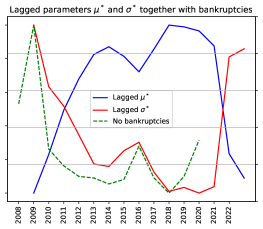
Figure 7: Time evolution of lagged parameters $\bm{\mu}^{*}$ and $\bm{\sigma}^{*}$ together with number of bankruptcies.

6 Conclusion

To the best of our knowledge, this research introduces for the first time the concept of multimodal learning in bankruptcy prediction models. We use the CMMD model to learn multimodal representations that embed information from different data modalities. These modalities, which describe the financial situation of a company from different angles, are accounting, market, and MDA data. The MDA data are not available for all firms. The advantage of the CMMD model is that after using all three modalities for model training, it only needs access to accounting and market modalities during test time. Therefore, this model solves the limitation of previous bankruptcy models using textual data, which can only make predictions for companies for which the MDA information is available.

The empirical results of this research show that if the training data set is large enough, our proposed methodology outperforms a large number of traditional classifier models.

7 Aknowledgments

We thank Sudheer Chava and Feng Mai for sharing the bankruptcy and MDA data with us, respectively.

8 Appendix

We fine-tune the hyperparameters of all models used in this research. Table 6 shows the parameters considered in the grid search approach.

Table 6: Grid search for hyperparameter tuning for all models studied in this research. We consider all combinations of the hyperparameters listed here. The superscripts *, **, and *** denote the best architecture for 1, 2, and 3 years bankruptcy predictions, respectively (see Table 5). Likewise, the subscript **** denotes the best architecture used in the experiments shown in Table 4. For the rest of hyperparamters in the benchmark models, we used default values in the sklearn implementation.

Hyperparameter	CMMD
latent dimension	50∗,∗∗,∗∗∗, 100, 150, 250∗∗∗∗
dropout encoder, prior, decoder	0∗∗∗,∗∗∗∗, 0.1∗,∗∗
layer size classifier	[50,50]∗∗∗, [100,100]∗∗∗∗, [150,150]∗,∗∗
layer size encoder, prior, decoder	[50,50,50]∗∗∗∗, [100,100,100]∗,∗∗,∗∗∗
omega	0.25, 0.5, 0.75∗,∗∗,∗∗∗, 0.9∗∗∗∗
	RF
no. of trees	50∗,∗∗, 100∗∗∗, 150, …, 450∗∗∗∗, …, 900, 950, 1000
max. depth of the tree	10∗∗∗∗, 20∗∗, …, 40∗, 50∗∗∗, …, 100, 110
no. of features when splitting	auto∗,∗∗,∗∗∗∗, sqrt∗∗∗
min. no. of samples to split an internal node	2, 5∗∗,∗∗∗,∗∗∗∗, 10∗
min. no. of samples to be at a leaf node	1∗∗,∗∗∗, 2, 4∗,∗∗∗∗
bootstrap	True∗,∗∗,∗∗∗,∗∗∗∗, False
	SVM
regularization parameter	0.1, 0.5, 1, 5∗∗∗∗, 10∗,∗∗,∗∗∗
kernel	linear, rbf∗,∗∗,∗∗∗,∗∗∗∗
kernel coefficient	scale∗,∗∗,∗∗∗,∗∗∗∗, auto
	MLP
layer size	10∗∗∗∗, 20, 50, 100, [10,10], [20,20]∗,∗∗∗, [50,50], [100,100]∗∗
activation function	logistic, tanh∗∗∗, relu∗,∗∗,∗∗∗∗
learning rate	constant∗,∗∗∗∗, invscaling∗∗∗, adaptive∗∗
L2 regularization	0.0001∗,∗∗, 0.001∗∗∗, 0.01, 1∗∗∗∗
	k-NN
no. of neighbors	3,5,10,15,20,30∗∗∗,50,80,110∗∗∗∗,150∗,∗∗,200,300
weight function for predictions	uniform, distance∗,∗∗,∗∗∗,∗∗∗∗
distance metric	euclidean∗∗∗∗, manhattan∗,∗∗,∗∗∗, minkowski
	NB
prior class probabilities	[0.5, 0.5]∗,∗∗∗,∗∗∗∗, [0.97, 0.03]∗∗
	LR
penalty	l2, l1∗,∗∗,∗∗∗,∗∗∗∗
inverse of regularization	0.0001, 0.001, 0.01, 0.1, 0.5∗∗∗∗, 1, 5, 10∗, 15, 20, 50∗∗,∗∗∗

References

- Alaka et al. (2018) Hafiz A Alaka, Lukumon O Oyedele, Hakeem A Owolabi, Vikas Kumar, Saheed O Ajayi, Olugbenga O Akinade, Muhammad Bilal. Systematic review of bankruptcy prediction models: Towards a framework for tool selection. Expert Systems with Applications, 2018, 94:164–184.
- Alfaro et al. (2008) Esteban Alfaro, Noelia García, Matías Gámez, David Elizondo. Bankruptcy forecasting: An empirical comparison of adaboost and neural networks. Decision Support Systems, 2008, 45(1):110–122.
- Altman (1968) Edward I. Altman. Financial ratios, discriminant analysis and the prediction of corporate bankruptcy. The Journal of Finance, 1968, 23(4):589–609.
- Atiya (2001) Amir F Atiya. Bankruptcy prediction for credit risk using neural networks: A survey and new results. IEEE Transactions on neural networks, 2001, 12(4):929–935.
- Bali et al. (2016) Turan G Bali, Robert F Engle, Scott Murray. Empirical asset pricing: The cross section of stock returns. John Wiley & Sons, 2016.
- Baltrušaitis et al. (2018) Tadas Baltrušaitis, Chaitanya Ahuja, Louis-Philippe Morency. Multimodal machine learning: A survey and taxonomy. IEEE transactions on pattern analysis and machine intelligence, 2018, 41(2):423–443.
- Barniv et al. (1997) Ran Barniv, Anurag Agarwal, Robert Leach. Predicting the outcome following bankruptcy filing: a three-state classification using neural networks. Intelligent Systems in Accounting, Finance & Management, 1997, 6(3):177–194.
- Beaver (1966) William H Beaver. Financial ratios as predictors of failure. Journal of accounting research, 1966, pp. 71–111.
- Bell et al. (1990) Timothy B Bell, Gary S Ribar, Jennifer Verichio. Neural nets versus logistic regression: A comparison of each model’s ability to predict commercial bank failures. 1990.
- Bengio et al. (2013) Yoshua Bengio, Aaron Courville, Pascal Vincent. Representation learning: A review and new perspectives. IEEE transactions on pattern analysis and machine intelligence, 2013, 35(8):1798–1828.
- Berg (2007) Daniel Berg. Bankruptcy prediction by generalized additive models. Applied Stochastic Models in Business and Industry, 2007, 23(2):129–143.
- Berns et al. (2022) John Berns, Patty Bick, Ryan Flugum, Reza Houston. Do changes in md&a section tone predict investment behavior? Financial Review, 2022.
- Blei et al. (2017) David M Blei, Alp Kucukelbir, Jon D McAuliffe. Variational inference: A review for statisticians. Journal of the American statistical Association, 2017, 112(518):859–877.
- Boritz et al. (1995) J Efrim Boritz, Duane B Kennedy, Augusto de Miranda e Albuquerque. Predicting corporate failure using a neural network approach. Intelligent Systems in Accounting, Finance and Management, 1995, 4(2):95–111.
- Cecchini et al. (2010) Mark Cecchini, Haldun Aytug, Gary J Koehler, Praveen Pathak. Making words work: Using financial text as a predictor of financial events. Decision Support Systems, 2010, 50(1):164–175.
- Chauhan et al. (2009) Nikunj Chauhan, Vadlamani Ravi, D Karthik Chandra. Differential evolution trained wavelet neural networks: Application to bankruptcy prediction in banks. Expert Systems with Applications, 2009, 36(4):7659–7665.
- Chava (2014) Sudheer Chava. Environmental externalities and cost of capital. Management science, 2014, 60(9):2223–2247.
- Cho and Muslu (2021) Hyunkwon Cho, Volkan Muslu. How do firms change investments based on md&a disclosures of peer firms? The Accounting Review, 2021, 96(2):177–204.
- Chung and Tam (1993) Hyung-Min Michael Chung, Kar Yan Tam. A comparative analysis of inductive-learning algorithms. Intelligent Systems in accounting, finance and management, 1993, 2(1):3–18.
- Coats and Fant (1993) Pamela K Coats, L Franklin Fant. Recognizing financial distress patterns using a neural network tool. Financial management, 1993, pp. 142–155.
- Demyanyk and Hasan (2010) Yuliya Demyanyk, Iftekhar Hasan. Financial crises and bank failures: A review of prediction methods. Omega, 2010, 38(5):315–324.
- Ding et al. (2012) A. Adam Ding, Shaonan Tian, Yan Yu, Hui Guo. A Class of Discrete Transformation Survival Models With Application to Default Probability Prediction. Journal of the American Statistical Association, 2012, 107(499):990–1003.
- Doersch (2016) Carl Doersch. Tutorial on variational autoencoders. arXiv preprint arXiv:1606.05908, 2016.
- Durnev and Mangen (2020) Art Durnev, Claudine Mangen. The spillover effects of md&a disclosures for real investment: The role of industry competition. Journal of Accounting and Economics, 2020, 70(1):101299.
- Etheridge and Sriram (1997) Harlan L Etheridge, Ram S Sriram. A comparison of the relative costs of financial distress models: artificial neural networks, logit and multivariate discriminant analysis. Intelligent Systems in Accounting, Finance & Management, 1997, 6(3):235–248.
- Fanning and Cogger (1994) Kurt M Fanning, Kenneth O Cogger. A comparative analysis of artificial neural networks using financial distress prediction. Intelligent Systems in Accounting, Finance and Management, 1994, 3(4):241–252.
- Fletcher and Goss (1993) Desmond Fletcher, Ernie Goss. Forecasting with neural networks: an application using bankruptcy data. Information & Management, 1993, 24(3):159–167.
- Hand (2009) David J Hand. Measuring classifier performance: a coherent alternative to the area under the roc curve. Machine learning, 2009, 77(1):103–123.
- Huang (2008) Fu-yuan Huang. A genetic fuzzy neural network for bankruptcy prediction in chinese corporations. In 2008 International Conference on Risk Management & Engineering Management, pp. 542–546. IEEE, 2008.
- Iturriaga and Sanz (2015) Félix J López Iturriaga, Iván Pastor Sanz. Bankruptcy visualization and prediction using neural networks: A study of us commercial banks. Expert Systems with applications, 2015, 42(6):2857–2869.
- Jain and Nag (1997) Bharat A Jain, Barin N Nag. Performance evaluation of neural network decision models. Journal of Management Information Systems, 1997, 14(2):201–216.
- Jeong et al. (2012) Chulwoo Jeong, Jae H Min, Myung Suk Kim. A tuning method for the architecture of neural network models incorporating gam and ga as applied to bankruptcy prediction. Expert Systems with Applications, 2012, 39(3):3650–3658.
- Kim and Yoon (2021) Alex Gunwoo Kim, Sangwon Yoon. Corporate bankruptcy prediction with domain-adapted bert. EMNLP 2021, 2021, p. 26.
- Kim and Kang (2010) Myoung-Jong Kim, Dae-Ki Kang. Ensemble with neural networks for bankruptcy prediction. Expert systems with applications, 2010, 37(4):3373–3379.
- Kingma and Ba (2014) Diederik P Kingma, Jimmy Ba. Adam: A method for stochastic optimization. arXiv preprint arXiv:1412.6980, 2014.