CardiacGen: A Hierarchical Deep Generative Model for Cardiac Signals

Abstract

We present CardiacGen, a Deep Learning framework for generating synthetic but physiologically plausible cardiac signals like ECG. Based on the physiology of cardiovascular system function, we propose a modular hierarchical generative model and impose explicit regularizing constraints for training each module using multi-objective loss functions. The model comprises 2 modules, an HRV module focused on producing realistic Heart-Rate-Variability characteristics and a Morphology module focused on generating realistic signal morphologies for different modalities. We empirically show that in addition to having realistic physiological features, the synthetic data from CardiacGen can be used for data augmentation to improve the performance of Deep Learning based classifiers. CardiacGen code is available at https://github.com/SENSE-Lab-OSU/cardiac_gen_model.

1 Introduction

There are many Machine Learning (ML) algorithms that use physiological signals like Electrocardiogram (ECG) for useful inference tasks such as biometrics (Rathore et al., 2020), Heart-Rate prediction (Reiss et al., 2019) and stress detection (Schmidt et al., 2018). However, the publicly available datasets are limited in size, especially for training large-scale data-driven Artificial Neural Networks (ANN) models. Moreover, collecting data at abnormal physiological conditions such as extreme Heart-Rates and Stress have practical limitations since most people usually have normal physiological conditions. Therefore, there is a potential for creating synthetic training data to improve performance of such Deep Learning (DL) models through data-augmentation. Alternatively, data-augmentation can be interpreted as an indirect method to incorporate domain knowledge into the learning process through this synthetic data. While some parametric models of the data-generation process have been suggested for cardiac signals (McSharry et al., 2003; Jafarnia-Dabanloo et al., 2007; Zeeman, 1973; Roy et al., 2020), they have limitations especially for augmenting datasets as shown by Golany et al. (2020). This is expected as it is difficult to capture the complexity of interactions in biological dynamical systems such as our cardiovascular system.

ANN-based Generative Adversarial Networks (GAN) proposed by Goodfellow et al. (2014) are a possible data-driven solution for data-augmentation, but this immediately raises a question. If the training dataset isn’t large enough to learn a DL classifier, how will we use it to learn a GAN? Since generative models like GANs try to approximate the data-generating process, we can better regularize by incorporating domain knowledge into them, e.g. through appropriate loss functions. Such data-driven models have received much attention recently (Kuznetsov et al., 2020; Zhu et al., 2019; Delaney et al., 2019; Golany et al., 2020).

Unlike existing DL methods, we use the knowledge about Heart Rate Variability (HRV) characteristics and pulse morphological properties of cardiac signals to create a modular generative model called CardiacGen (short for Cardiac-signal-Generator). CardiacGen comprises two ANN modules based on Wasserstein GANs with gradient-penalty (WGAN-GP) (Gulrajani et al., 2017) and its modular design has many advantages described in the following section 2. In addition to being used in conventional simulator applications such as simulated testing of algorithms and privacy preservation, CardiacGen can be employed to produce cardiac signals under rarely observed physiological conditions (e.g. very low/high heart rates) and to transcode from one cardiac modality to another. Moreover, it can enrich existing datasets by generating samples for underrepresented population groups, potentially reducing health disparities (Martin et al., 2019; Gao and Cui, 2020). However, we’ll focus on data-augmentation as its primary application in this paper.

Formal definitions of terms Data-Augmentation and Conditional Generative Modeling, as used in the context of this paper, are provided in appendix Section A. Next, we describe important notation used throughout the text. The lower-case character $x$ represents a fixed sample value of a random vector (rv) $X$ (the corresponding upper-case character), $M:N$ is the enumeration of natural numbers from $M$ to $N$, $g(X_{1:N};w)$ denotes function $g$ of rv’s $X_{1:N}$ with deterministic parameters $w$ and an index-based $x[v]$ represents the $v^{th}$ value from the ordered set $\{x[i]:i\in\{1:N\}\}$.

Our aim is to design a data-augmenting transformation $A$ as an ANN-based conditional generative model $CG$ with parameters $w_{CG}$, that generates random samples of $X$ (a cardiac signal like ECG) conditioned on some $Y$ and a latent rv $Z$, i.e. sampling from $CG(Y,Z;w_{CG})$ must be a good approximation of sampling from $p(X|Y)$. The dataset of all samples is split into 3 subsets $\mathcal{D}_{train}$, $\mathcal{D}_{val}$ and $\mathcal{D}_{test}$ for model training, cross-validation and evaluation respectively. To augment $\mathcal{D}_{train}$, for every $y\in\mathcal{D}_{train}$ we use $CG$ to generate $N$ new samples $(CG(y)[k],y)_{k=1}^{N}$ where $CG(y)[k]$ denotes $k^{th}$ stochastic sample of $CG(y)$.

2 Method

The human heart consists of 4 chambers, the upper two called atria and lower two called ventricles. The right two chambers pump deoxygenated blood and the left two chambers pump oxygenated blood. For doing this, the heart goes through a cardiac cycle of contraction (called systole) and relaxation (called diastole). The timing of contraction and relaxation events is triggered by electrical signals originating in specialized cells of the Sino-Atrial (SA) node. Hence, all 4 chambers undergo corresponding depolarization/repolarization cycles which form the characteristic morphology comprising peaks and valleys of an ECG signal labeled as P, Q, R, S, and T (refer appendix Figure LABEL:fig:cg.ECG_morph). The R-peak is the greatest absolute magnitude point in the signal and is commonly used to locate the cardiac cycles in the ECG signal. The interval between consecutive R-peaks is called the RR-interval. Instantaneous Heart Rate (HR) is defined as the inverse of RR-interval.

Notably, the timing of the SA node is in turn controlled by sympathetic and parasympathetic systems of the Autonomic Nervous System. This forms the basis of inter-beat interval variations known as Heart Rate Variability (HRV). All low-frequency (LF) variations (0.04-0.15 Hz.) are caused by the sympathetic system while high-frequency (HF) modulations (0.15-0.4 Hz.) are caused by both systems, though predominantly by the parasympathetic system.

Based on this knowledge of the heart’s physiology, we modularize the CardiacGen model $CG$ into 2 ANN based modules, $CG_{HRV}$ and $CG_{Morph}$. This imposes a hierarchical structure to the function class in addition to creating a meaningful intermediate representation. As the names suggest, $CG_{HRV}$ models HRV characteristics while $CG_{Morph}$ models morphological properties. It is also important to be able to extract and condense HRV features from cardiac signal $X$ (ECG) into a uniformly resampled RR-tachogram representation (Electrophysiology, 1996) $X_{HRV}[i]=R[i]-R[i-1]$ where $R[i]$ denotes the time of $i^{th}$ R-peak occurrence in seconds. $X_{HRV}$ is further low-pass filtered with a cutoff frequency of 0.5 Hz. to remove noise. This enables training of the $CG_{HRV}$ module. There are several advantages of such modularization including:

1. Ability to enforce signal properties via penalty terms in the loss function.

2. May help in privacy preservation applications by enabling masking of HRV or morphological characteristics that might be used to identify subjects.

3. Meaningful intermediate representation of RR-tachogram adds interpretability and can help locate the problematic module in case of a training failure.

4. Train smaller models (both modules) with fewer parameters compared to a large end-to-end model and with projections of the training data tailored to appropriate time-scale.

5. May enable signal imputation and signal transcoding, e.g. obtaining Photoplethysmogram (PPG) from ECG using $CG_{Morph}$.

6. HRV module will facilitate easier knowledge transfer to new datasets because RR-tachogram representation is robust to most data-set variations.

We use the publicly available WESAD dataset (Schmidt et al., 2018) for training CardiacGen. Details of the dataset are described in appendix Section B.1. The windows of ECG signal being modeled are referred as $X$. Conditioning vector $Y$ is the concatenation of one-hot representations of available emotion labels $Y_{emo}$, identity labels $Y_{id}$ and a conditioning signal $X_{avgHRV}$ or $X_{peak}$ described in the next section.

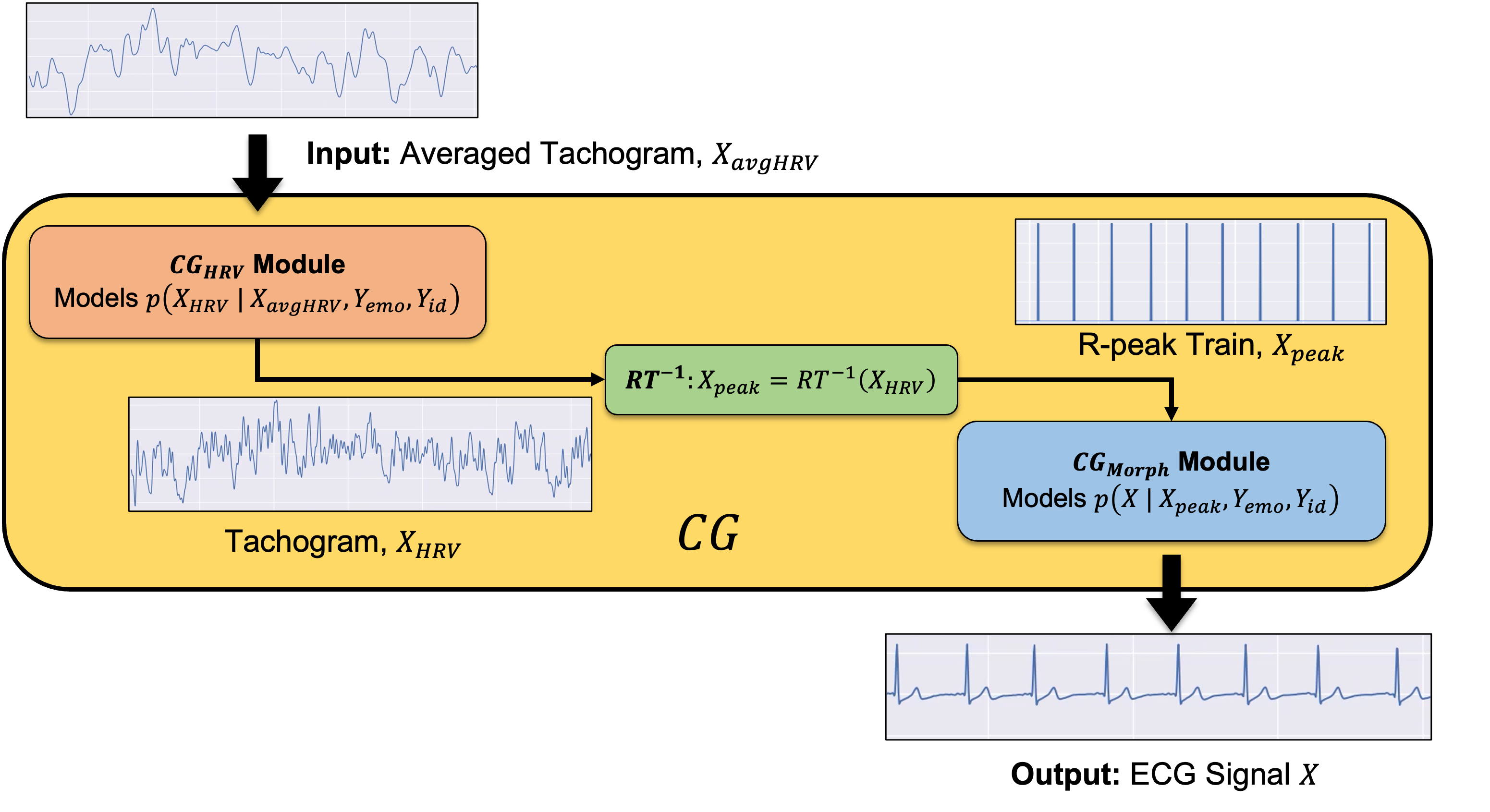
[CardiacGen Model] [Continuity Aware Training]

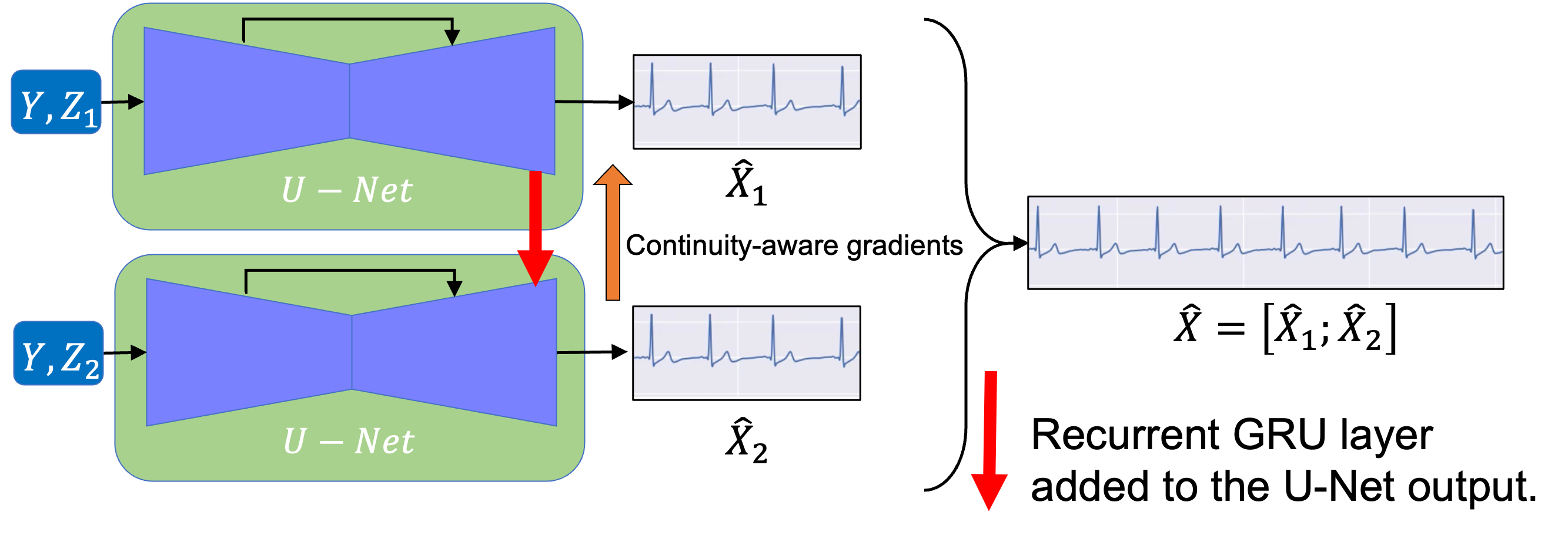
Figure 1: Schematics for CardiacGen Model and continuity aware training of the generators.

3 Model

CardiacGen consists of two ANNs, the HRV module $CG_{HRV}(Y_{HRV},Z_{HRV};w_{HRV})$ which creates samples from $p(X_{HRV}|Y_{HRV})$ and the Morphology module
$CG_{Morph}(Y_{Morph},Z_{Morph};w_{Morph})$ which creates samples from $p(X|Y_{Morph})$ as shown in Figure 1. Here, $Y_{HRV}=[X_{avgHRV};Y_{emo};Y_{id}]$, $Y_{Morph}=[X_{peak};Y_{emo};Y_{id}]$, notation $[u;v]$ represents concatenation of vectors $u$ and $v$. $X_{avgHRV}$ is obtained from the uniformly resampled RR-tachogram and low-pass filtering it to 0.125 Hz. cutoff frequency and $X_{peak}$ is the R-peak train i.e. a binary-valued signal with 1’s at R-peak locations else 0’s. Both $Z_{HRV},Z_{Morph}\sim\mathcal{N}(0,I)$ as in a conventional GAN.

$X_{avgHRV}$ is chosen as an input condition to $CG_{HRV}$ since it represents Low-Frequency (LF) properties of $X_{HRV}$ which remain fairly consistent across subjects. This allows for the desired sampling for augmentation (See appendix Section B.3). $X_{peak}$ is chosen as an input condition to $CG_{Morph}$ because, in our perspective, it is a more conducive input representation for $CG_{Morph}$. Going from $X_{peak}$ to the pulsatile ECG $X$ can be viewed as finding a time-varying non-linear filter. The transformation $RT:X_{HRV}=RT(X_{peak})$ is fully determined and used at training time to obtain training samples. But at inference time, the inverse transformation $X_{peak}=RT^{-1}(X_{HRV})$ is under-determined. So we constrain it by placing the last 1 uniform-randomly in the last 0.25 seconds (s.) of $X_{peak}$ and using $X_{HRV}$ curve to get the previous R-peak locations henceforth.

Both $CG_{HRV}$ and $CG_{Morph}$ modules consist of WGAN-GP (Gulrajani et al., 2017). WGAN-GP was chosen because of its advantages over traditional GANs, especially meaningful loss curves for cross-validation and reliable training. WGAN-GP requires an extra critic ANN $D(\cdot,\cdot;w_{D})$ to be learned simultaneously to aid the learning of the distribution approximators (or generators). Both, the critic and generators are trained alternately using gradient descent steps. Regularizing loss terms are added to the loss functions used for training generators of both modules. A Power Spectral Density (PSD) reconstruction loss $\mathcal{L}_{PSD}$ is added to the loss function $\mathcal{L}_{HRV}$ of $CG_{HRV}$ as shown in appendix eq. 1. Similarly, a mean-squared reconstruction loss $\mathcal{L}_{MSE}$ is added to loss function $\mathcal{L}_{Morph}$ of $CG_{Morph}$ as shown in appendix eq. 2. The WGAN $\mathcal{L}_{W}$ and gradient-penalty $\mathcal{L}_{GP}$ parts of loss functions are from eq. 3 of Gulrajani et al. (2017) and the complete description of loss functions is provided in appendix Section B.

Inspired by the seminal work of Isola et al. (2017), the generators of both modules have a U-Net style architecture comprising convolutional layers. However, since we want to generate time-series of arbitrary durations, we do 2 modifications. We add a Recurrent Layer having Gated-Recurrent-Unit (GRU) cells at the output of the U-Net. This can be viewed as non-linear filtering of features extracted by Convolutional layers and promotes continuity between outputs of consecutive windows as GRU states are propagated forward. Next, to further promote this continuity, we train 2 copies of the generator simultaneously where the second copy uses the GRU state from the first as shown in Figure 1.

4 Experimental Setup

We use the Tensorflow (2.1) (Abadi et al., 2016) for our implementations. More details of software and hardware used can be found in appendix section B. The data pre-processing for training and post-processing for results in Section 5 are described in appendix Sections B.2 and B.3 respectively. Although CardiacGen has multiple use-cases as described in Section 2, we’ll evaluate its utility by its ability of data-augmentation. To this end, we implement and train two supervised ANN multi-class classifiers from recent state-of-the-art works by Sarkar and Etemad (2021) and Donida Labati et al. (2019). $g_{emo}$ is a 4-class classifier (neutral, stress, amusement, and meditation) for emotion recognition based on the former, and $g_{id}$ is a 15-class classifier (identifying every subject) for identity recognition based on the latter. Since HRV features are more important for emotion recognition (Hovsepian et al., 2015; Schmidt et al., 2018) while morphological features are essential for identity recognition, this strategy helps evaluate both modules. Additional details of training these classifiers are provided in the appendix Section B.4.

5 Results

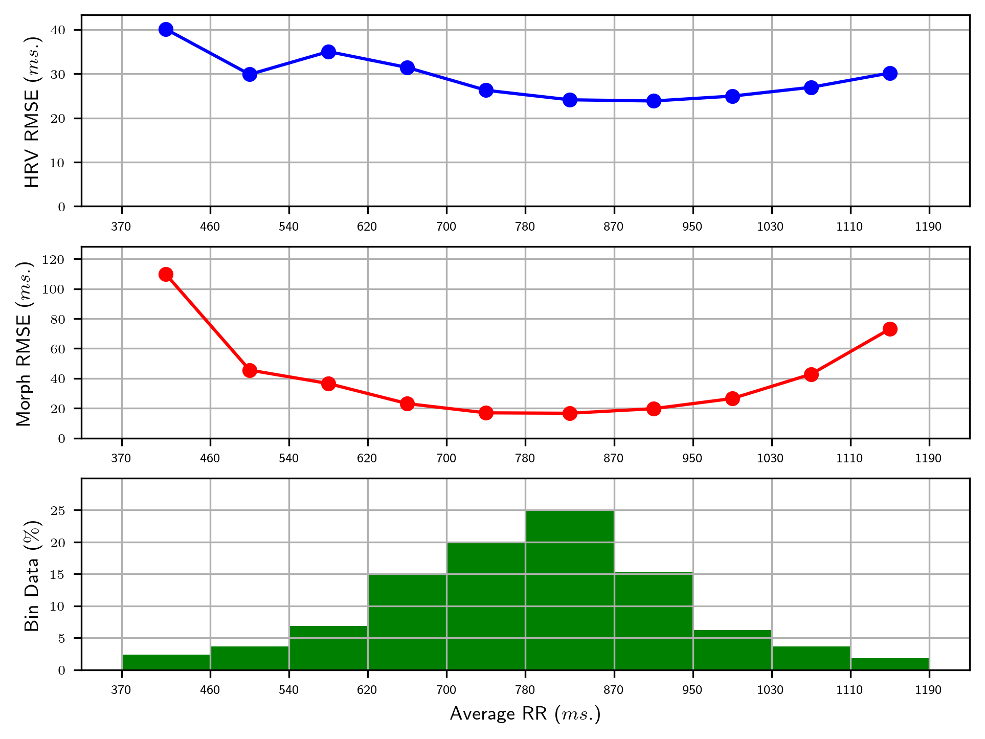
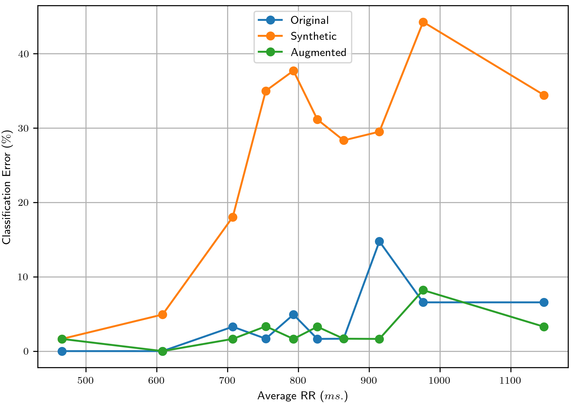
fig:cg.res [Conditional Generation Ability] [RMSSD for subjects S13 to S17]
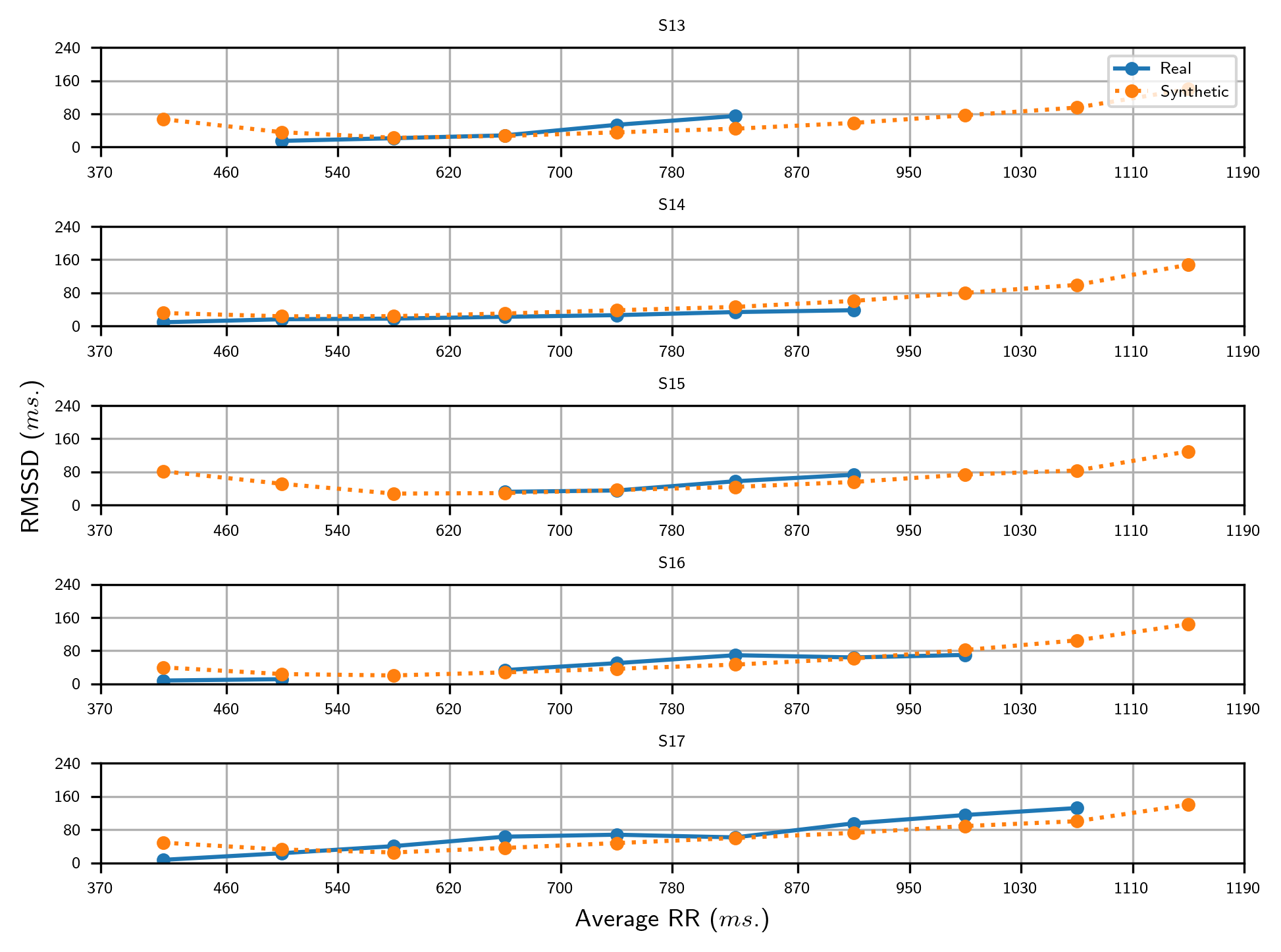
[Test Error for Emotion Recognition] [Test Error for Identity Recognition]

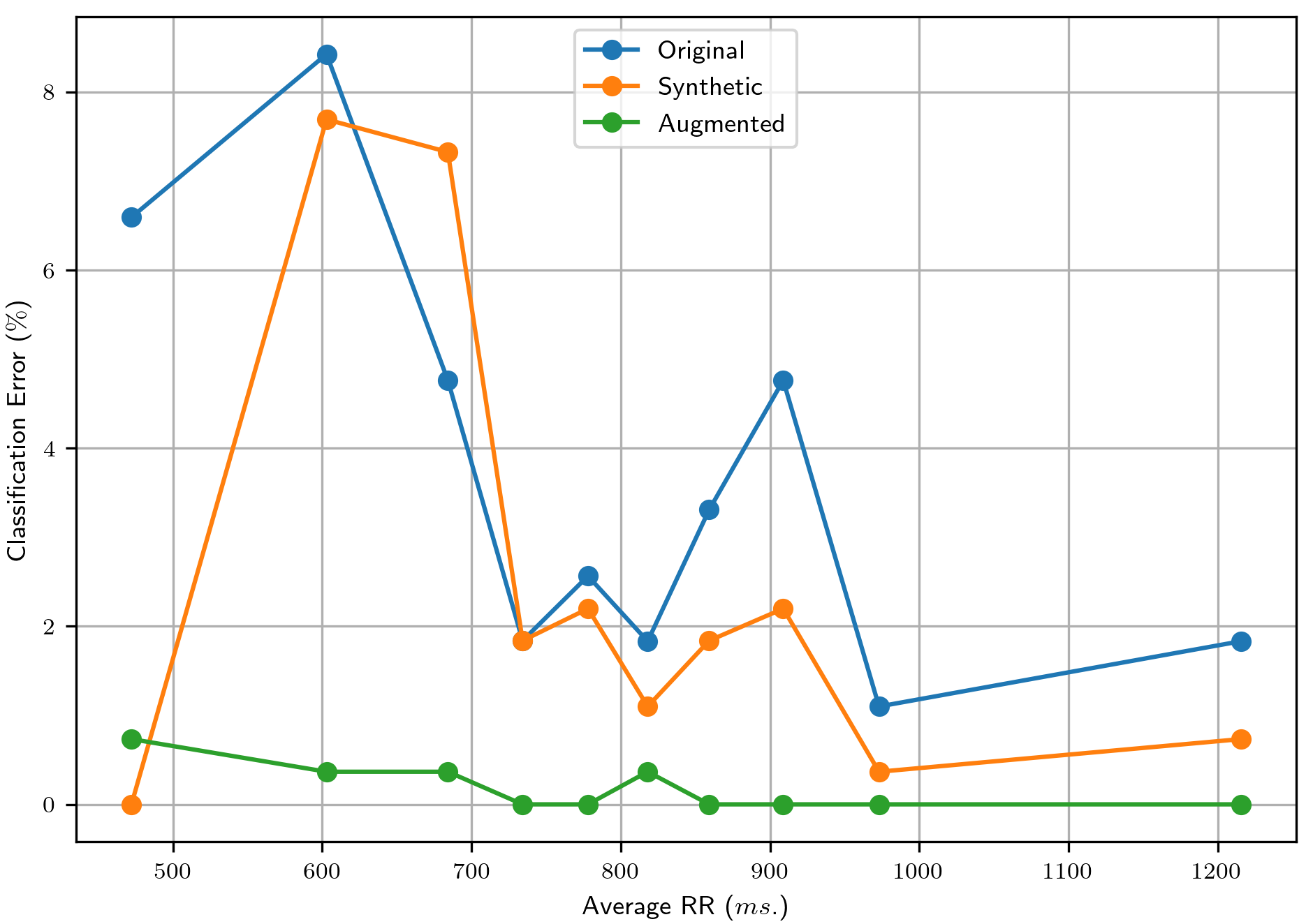
Figure 2: Evaluating various aspects of CardiacGen

In this section, we evaluate CardiacGen based on three quantitative criteria. We first test whether the generated output of both CardiacGen modules actually follows the input real-valued condition. For this, we use the synthetically generated $X_{HRV}$ and ECG to re-derive synthetic $X_{avgHRV}$ and $X_{HRV}$ from $CG_{HRV}$ and $CG_{Morph}$ modules respectively. We then find the root-mean-squared-error (RMSE) between these synthetically re-derived signals and their real counterparts that were used as input conditions (in ms.). For Figure 2, further bin these RMSE values based on the Average RR length of every window and report the mean RMSE in every bin. It is evident from Figure 2 that a significant majority of windows have RMSE lower than 30 ms. for both modules. The overall average RMSE for $CG_{HRV}$ is 27 ms. and for $CG_{Morph}$ is 25 ms. Hence, both modules, and consequently, CardiacGen, retains information about the real-valued condition vectors well. The further evaluation of utility will provide a proxy estimate of conditional generation ability with respect to the categorical condition vectors.

Next, we verify whether CardiacGen synthesizes realistic physiological data by calculating HRV feature RMSSD (Shaffer and Ginsberg, 2017) for 32 s windows of data and binning them as earlier. Effectiveness of our method is demonstrated from Figure 2 as the empirical distributions of RMSSD from real and synthetic data are fairly close for all subjects. The smaller support (i.e. missing bin values) of a subject’s real-data can be explained as follows. A subject experiences only one sequence of HR during real-data collection while we obtained synthetic data with HR of other subjects as well, thus increasing its variety. Results for remaining subjects are provided in appendix section C.

The utility of the synthetic ECG from CardiacGen is measured in terms of its ability to learn ANN models for two classification tasks, emotion and identity recognition. All the test results use samples from the unseen $\mathcal{D}_{test}$ after training the classifiers. The values reported are classification errors, i.e., the percentage of samples misclassified. Graphs show variations across 10 equally-sized HR bins (i.e. same no. of samples in each bin).

It is evident from Figure 2 that the augmented dataset gives the smallest errors in all bins except one. Even while training entirely on synthetic data $\mathcal{D}_{synth}$, the errors are much lower than the random chance error of $75\%$. The overall test errors (in %) are 4.04, 28.08, and 2.8 when training using datasets $\mathcal{D}_{train}$, $\mathcal{D}_{synth}$ and $\mathcal{D}_{aug}$ respectively. Hence, we achieve more than 30% improvement after augmentation. Compared with the results of Sarkar and Etemad (2021), our classification results establish new state-of-the-art accuracy for the Affect recognition task using the WESAD dataset. Although we used the same size of test-set as Sarkar and Etemad (2021), we use a fixed test-set instead of the 10-fold cross-validation done by Sarkar and Etemad (2021) which is a limitation of our evaluation. This was done to make training feasible for all models, in our limited computation and time resources.

Figure 2 further shows the significance of synthetic data from CardiacGen in improving identity recognition performance. In fact, just using synthetic data from CardiacGen is at par with using real data in $\mathcal{D}_{train}$. The overall test errors (in %) are 1.03, 1.94, 0.18 when using datasets $\mathcal{D}_{train}$, $\mathcal{D}_{synth}$ and $\mathcal{D}_{aug}$ respectively. Hence, we get more than 82% improvement after augmentation.

6 Conclusion

We proposed a generative model, CardiacGen, for generating synthetic cardiac signals. We demonstrated the model’s ability to produce physiologically plausible signals as well as its ability to augment datasets. However, the effect of the stochastic latent variable $Z$ on CardiacGen’s output is negligible. As a result, the conditional variance of CardiacGen is smaller than the variance observed in measured signals. This was observed in pix2pix (Isola et al., 2017) as well. Moreover, the WESAD dataset used for training has a limited size and lacks age as well as gender diversity. In future work, we plan to improve on these limitations through additional regularization terms, diverse training datasets as well as extend CardiacGen to generate other cardiac signals like PPG, and explore signal transcoding applications e.g. converting ECG to PPG signals. This research was partially supported by NSF grants CNS-1823070 CBET-2037398 and NIH Grant P41EB028242

Appendix A Definitions

Definition A.1 (Data Augmentation).

Data Augmentation involves applying an appropriate transformation $A:\mathcal{D}_{in}\rightarrow\mathcal{D}_{out}$ to a training data-set $\mathcal{D}_{train}$ and expand it to an augmented data-set $\mathcal{D}_{aug}=A(\mathcal{D}_{train})$. The aim is to find $A$ such that the estimated parameters $w$ for a supervised learning problem $\mathcal{P}$ using $\mathcal{D}_{aug}$, i.e., $w_{aug}=\mathcal{P}(\mathcal{D}_{aug})$ perform better than $w_{train}=\mathcal{P}(\mathcal{D}_{train})$ in terms of the chosen real-valued scalar performance measure $\mathcal{M}$.

Definition A.2 (Conditional Generative Modeling).

It aims to estimate the conditional distribution $p(X|Y)$ using a parameterized distribution family $q(X|Y;w)$ and a set of samples $\mathcal{D}$ from the joint distribution $p(X,Y)$ of random vectors $X,Y$. Since $X$ may depend on other factors of variation in addition to $Y$, there is inherent stochasticity in the generation of $X$ from $Y$. This is typically achieved by sampling a latent random vector $Z$, internal to $q(X|Y;w)$, which has a simpler distribution (e.g. standard Gaussian). Therefore, the goal is to generate $N$ realistic samples $\{x[v]\}_{v=1}^{N}$ from $q(X|Y;w)$ as if they were from $p(X|Y)$.

fig:cg.ECG_morph

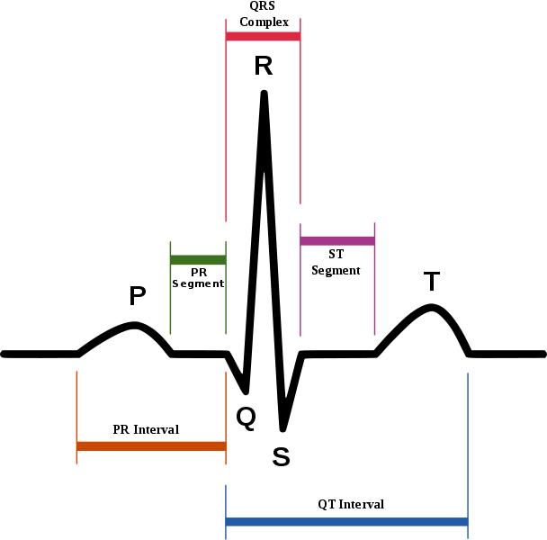
Figure 3: ECG morphology (by Agateller, 2007)

Appendix B Experimental Details

The complete loss functions used for training CardiacGen are as follows.

$$\mathcal{L}_{HRV} =\begin{cases}-\mathcal{L}_{W}+\lambda_{1}\mathcal{L}_{GP}&\text{for }D_{HRV}\\ \mathcal{L}_{W}+\lambda_{2}\mathcal{L}_{PSD}&\text{for }CG_{HRV}\end{cases}$$ (1)

$$\mathcal{L}_{Morph} =\begin{cases}-\mathcal{L}_{W}+\lambda_{1}\mathcal{L}_{GP}&\text{for }D_{Morph}\\ \mathcal{L}_{W}+\lambda_{3}\mathcal{L}_{MSE}&\text{for }CG_{Morph}\end{cases}$$ (2)

$$\mathcal{L}_{W} =\operatorname{\mathbb{E}}_{y}\left[\operatorname{\mathbb{E}}_{x}\left[{D(x,y)}\right]-\operatorname{\mathbb{E}}_{\hat{x}}\left[{D(\hat{x},y)}\right]\right]$$

$$\mathcal{L}_{GP} =\operatorname{\mathbb{E}}_{(y,\bar{x})}\left[(\left\lVert{\nabla_{\bar{x}}D(\bar{x},y)}\right\rVert_{2}-1)^{2}\right]$$

$$\mathcal{L}_{PSD} =\operatorname{\mathbb{E}}_{y}\left[\operatorname{\mathbb{E}}_{(x,\hat{x})}\left[\vphantom{\frac{\left\lVert{\absolutevalue{\mathcal{F}(x)}^{2}}\right\rVert_{2}^{2}}{N_{\mathcal{F}}}}\right.\right.$$

$$\left.\left.W_{\mathcal{F}}\odot\frac{\left\lVert{\absolutevalue{\mathcal{F}(x)}^{2}-\absolutevalue{\mathcal{F}(\hat{x})}^{2}}\right\rVert_{2}^{2}}{N_{\mathcal{F}}}\right]\right]$$

$$\mathcal{L}_{MSE} =\operatorname{\mathbb{E}}_{y}\left[\operatorname{\mathbb{E}}_{(x,\hat{x})}\left[\left\lVert{x-\hat{x}}\right\rVert_{2}^{2}\right]\right]$$

where $y\sim p(Y)$, $x\sim p(X|y)$, $\hat{x}\sim q(X|y;w)$, $\bar{x}\sim r(\bar{X}|y)$ is uniform-sampling along straight lines between pairs of sampled points $x\sim p(X|y),\hat{x}\sim q(X|y;w)$, $\mathcal{F}$ denotes the Fourier transform operator, $N_{\mathcal{F}}$ is the length of the corresponding Fourier transform and $W_{\mathcal{F}}$ is a weighting used to emphasize HF components of the PSD. All expectations are approximated using corresponding empirical means. Motivated by Gulrajani et al. (2017), we employ negative critic loss as our primary metric for model selection. Hence, the weights of the final model are set to their values corresponding to the epoch where the smallest negative critic loss on $\mathcal{D}_{val}$ was achieved. For the hyperparameters, we use $\lambda_{1}=10$ (as in Gulrajani et al. (2017)) and set $\lambda_{2}=10^{-2}$, $\lambda_{3}=5$ to approximately balance the two regularizing loss terms $L_{PSD}$ and $L_{MSE}$ with the WGAN loss term $\mathcal{L}_{W}$ in magnitude. Unless mentioned otherwise, the Adam optimizer from Tensorflow with default parameters is used for most training runs, including the CardiacGen modules. NeuroKit2 (0.1.0) (Makowski et al., 2021) python library is used for various physiological signal processing, like R-peak detection and physiological feature estimation. We use NVIDIA GeForce RTX 2080 Ti GPU along-with Intel Xeon CPU as our primary computation hardware.

B.1 WESAD Dataset

Wearable Stress and Affect Dataset (WESAD) contains data from 15 subjects (12 males, 3 females) collected in a laboratory setting. The dataset has several physiological and motion sensor modalities from both a wrist-worn and a chest-worn device, but we’ll focus on using only ECG signals. We resample it from 700 Hz to 100 Hz and $X_{P}$ from 64 Hz to 25 Hz. The dataset also provides 5 emotion labels (0 = undefined/transient/irrelevant, 1 = baseline, 2 = stress, 3 = amusement, 4 = meditation) and 15 subject-ID labels. Note that we aggregated irrelevant emotion-labels 5/6/7 into 0 as well. We’ll use one-hot-representations $Y_{emo}\in\mathbb{R}^{5}$ of emotion labels and $Y_{id}\in\mathbb{R}^{15}$ of identity labels. WESAD has signals of approx.  90 minutes for each subject. The total duration of data used after pre-processing for ECG is 89,358 s. and the relative proportions of emotion labels {0,1,2,3,4} are {0.47,0.21,0.12,0.07,0.13} respectively.

B.2 Pre-Processing for Training CardiacGen

While constructing datasets $\mathcal{D}_{train}$, $\mathcal{D}_{val}$ and $\mathcal{D}_{test}$ for learning as well as evaluating DL models, we create segments/frames of window-length $win=8s.$ for ECG signals with a step-size $step=2s.$ These segmented input vectors are much more conducive to batch training than arbitrarily long signal vectors and we refer to the dataset of all such segments as $\mathcal{D}_{full}$.

While forming $\mathcal{D}_{val}$ and $\mathcal{D}_{test}$, it is challenging to maintain a variety of all signals. We adopt the following sampling strategy. We fix block size $bsize=13$ of consecutive segments for $\mathcal{D}_{test}$ and $\mathcal{D}_{val}$. Then for every subject’s $N_{id}$ signal segments, we sample $N_{bid}$ blocks of $bsize$ consecutive segments uniformly at random such that $N_{bid}\times bsize\approx 0.1\times N_{id}$ i.e. we select approx. $10\%$ segments. Let’s refer to this sampling process as $UD(N_{id},bsize)$. Hence, $\mathcal{D}_{test}$ is first constructed with test-segments from such a sampling. In addition to these test-segments, we drop the 6 overlapping terminal segments for every block of segments in $\mathcal{D}_{test}$ from $\mathcal{D}_{full}$ to ensure no data overlap further. From the remaining segments, we use the same sampling process $UD(N_{id},bsize)$ to get validation-segments and form $\mathcal{D}_{val}$. We only drop these selected validation segments from $\mathcal{D}_{full}$ and the remaining segments form the train segments of $\mathcal{D}_{train}$. Even though there is some overlap between validation and train segments, the majority of validation segments are non-overlapping which will ensure meaningful cross-validation results.

B.3 Post-Processing for Synthetic Data Generation

We describe our protocol to generate and use synthetic data in this section. We produce synthetic ECG data using the joint input condition $Y_{HRV}=[X_{avgHRV};Y_{emo};Y_{id}]$. $Y_{emo}$ and $Y_{id}$ are one-hot representations of class numbers sampled from the fixed sets $\{0:14\}$ and $\{1:4\}$ respectively. Although we use class 0 of $Y_{emo}$ during training, we don’t use it further as it comprises all irrelevant emotion labels. For $X_{avgHRV}$, $N_{CG}$ continuous windows $\{x_{avgHRV}[v]\}_{v=1}^{N_{CG}}$ can be sampled from the fixed set $HV_{\mathcal{D}}=\{x_{avgHRV}[u]\}_{u=1}^{N_{\mathcal{D}}}$ of all windows from corresponding real dataset $\mathcal{D}$. Thus, for each subject’s continuous windows of $X_{avgHRV}$, we produce synthetic data $\mathcal{D}_{synth}$ by using all $60$ possible permutations of $Y_{emo}$ and $Y_{id}$, i.e. $\mathcal{D}_{synth}$ is $60$ times the size of the corresponding real dataset $\mathcal{D}$.

The overall sampling process for generating synthetic ECG is then

$$x_{peak} =RT^{-1}\circ CG_{HRV}(y_{HRV},z_{HRV})$$ (3)

$$x_{E} =CG_{Morph}([x_{peak};y_{emo};y_{id}],z_{Morph})$$ (4)

For comparing the Physiological Features of real data with synthetic data, $\mathcal{D}_{full}^{32,0}$ consisting of all non-overlapping 32 s. windows of ECG is used as the Real Dataset and $HV_{\mathcal{D}_{full}^{32,0}}=\{x_{avgHRV}[u]\}_{u=1}^{N_{\mathcal{D}_{full}^{32,0}}}$ is used to produce corresponding synthetic dataset $\mathcal{D}_{synth}$. The reason for windowing as such is that HRV features of our interest are usually evaluated for windows of more than 30 s. in length (Kreibig, 2010). Since our sampling process of $\mathcal{D}_{synth}$ equally distributes all stress conditions 1 to 4 for every subject, $\mathcal{D}_{synth}$ is subject-wise sub-sampled such that the ratio of windows with stress conditions 1 to 4 is the same as in $\mathcal{D}_{full}^{32,0}$ of that subject. This is done so that HRV statistics used for further evaluation are comparable. The results are described in Section 5. Errors in the ECG R-peak detection algorithm cause several artificially high and low RR values beyond physiologically possible values. These outliers were present in both $\mathcal{D}_{train}$ and $\mathcal{D}_{synth}$. Removal of 0.5% smallest and 0.5% largest RR values help us to avoid these outliers for our evaluations. We note that the smaller $\mathcal{D}_{test}$ used for utility evaluation didn’t have any such outliers.

For comparing the utility of real ECG data and synthetic ECG data, $\mathcal{D}_{train}$ described above is used as the Real ECG training Dataset and $HV_{\mathcal{D}_{train}}=\{x_{avgHRV}[u]\}_{u=1}^{N_{\mathcal{D}_{train}}}$ is used to produce corresponding synthetic ECG training data $\mathcal{D}_{synth}$. Finally, we form the augmented training dataset $\mathcal{D}_{aug}=\mathcal{D}_{synth}\cup\mathcal{D}_{train}$ where both $\mathcal{D}_{synth}$ and $\mathcal{D}_{train}$ contain approximately same no. of samples obtained by simply repeating $\mathcal{D}_{train}$ samples appropriately. The same $\mathcal{D}_{val}$ is used for evaluation during all utility model-trainings and the same $\mathcal{D}_{test}$ is used for their evaluation after this utility-training. These post utility-training results are described in Section 5.

B.4 Training Deep Classifiers for assessing CardiacGen’s Utility

For ECG based emotion recognition classifier, data-preprocessing and ANN architecture are taken from Sarkar and Etemad (2021) with minor modifications for compatibility. ECG is over-sampled from 100 Hz to 256 Hz, i.e. from the sampling-rate we use to what the authors use. As suggested by the authors, we segment data into 10 s. windows.

For ECG based identity recognition classifier, data-preprocessing is kept almost the same as above and only the ANN architecture is taken from Donida Labati et al. (2019) with some modifications. A stride of 2 is added to all convolutional layers and Local Response Normalization (LRN) layers are replaced with Batch Normalization (BN) layers. We don’t derive feature vectors as in Donida Labati et al. (2019) and directly use signals themselves as inputs. We use signal windows of size 4 s. Since windows of size 10 s. have been shown to be sufficient for extracting stress indicating HRV features by Sarkar and Etemad (2021), the smaller size windows are used to make classifier focus on localized morphological properties for this closed-set-identification problem. Also, the identity recognition classifier are trained using Stochastic Gradient Descent optimizer with a learning rate of 0.001 and Nesterov-momentum of 0.6. All classifiers are trained using the standard categorical cross-entropy loss.

Appendix C Additional Results

fig:cg.res.feat.rmssd.app [Subjects S2 to S6]
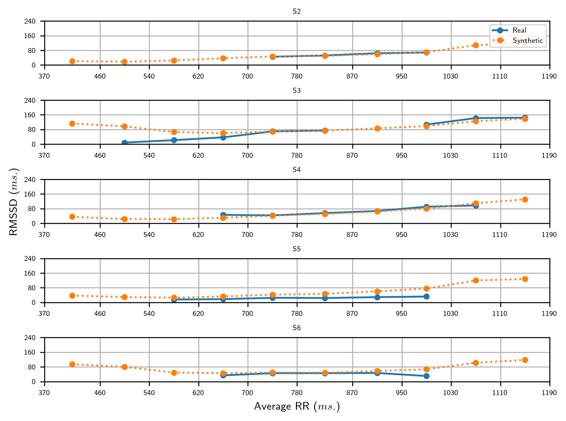
[Subjects S7 to S11]

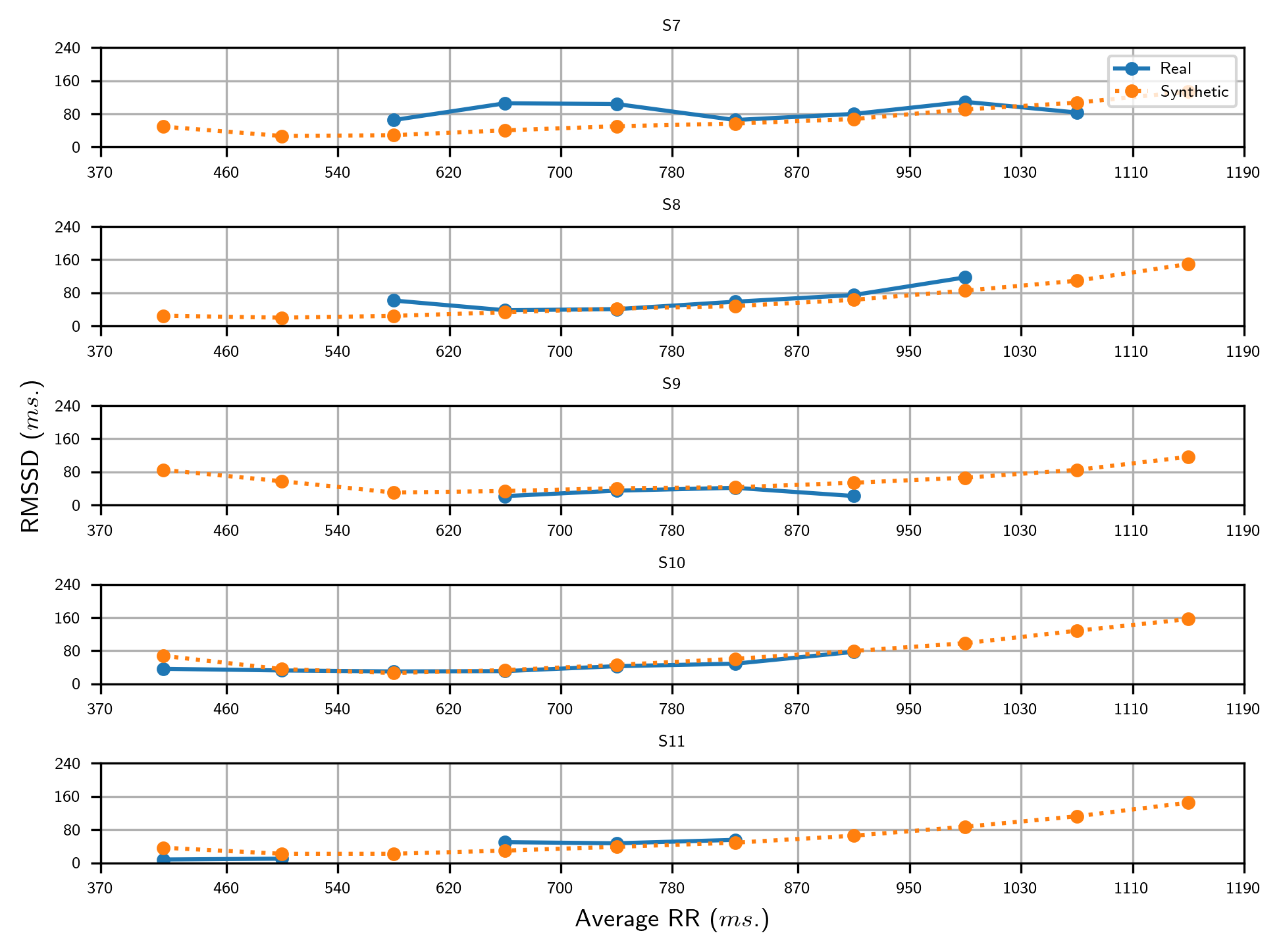
Figure 4: Evaluating HRV feature RMSSD

References

- Abadi et al. (2016) Martin Abadi, Paul Barham, Jianmin Chen, Zhifeng Chen, Andy Davis, Jeffrey Dean, Matthieu Devin, Sanjay Ghemawat, Geoffrey Irving, Michael Isard, Manjunath Kudlur, Josh Levenberg, Rajat Monga, Sherry Moore, Derek G. Murray, Benoit Steiner, Paul Tucker, Vijay Vasudevan, Pete Warden, Martin Wicke, Yuan Yu, and Xiaoqiang Zheng. {TensorFlow}: A System for {Large-Scale} Machine Learning. In 12th USENIX Symposium on Operating Systems Design and Implementation (OSDI 16), pages 265–283, 2016. ISBN 978-1-931971-33-1. URL https://www.usenix.org/conference/osdi16/technical-sessions/presentation/abadi.
- by Agateller (2007) Created by Agateller. Schematic diagram of normal sinus rhythm for a human heart as seen on ECG (with English labels)., 2007. URL https://commons.wikimedia.org/wiki/File:SinusRhythmLabels.svg.
- Delaney et al. (2019) Anne Marie Delaney, Eoin Brophy, and Tomas E. Ward. Synthesis of Realistic ECG using Generative Adversarial Networks. arXiv:1909.09150 [cs, eess, stat], September 2019. URL http://arxiv.org/abs/1909.09150.
- Donida Labati et al. (2019) Ruggero Donida Labati, Enrique Muñoz, Vincenzo Piuri, Roberto Sassi, and Fabio Scotti. Deep-ECG: Convolutional Neural Networks for ECG biometric recognition. Pattern Recognition Letters, 126:78–85, September 2019. ISSN 0167-8655. 10.1016/j.patrec.2018.03.028. URL https://www.sciencedirect.com/science/article/pii/S0167865518301077.
- Electrophysiology (1996) Task Force of the European Society of Cardiology the North American Society of Pacing Electrophysiology. Heart rate variability: Standards of measurement, physiological interpretation, and clinical use. Circulation, 93(5):1043–1065, 1996.
- Gao and Cui (2020) Yan Gao and Yan Cui. Deep transfer learning for reducing health care disparities arising from biomedical data inequality. Nature Communications, 11(1):5131, October 2020. ISSN 2041-1723. 10.1038/s41467-020-18918-3. URL https://www.nature.com/articles/s41467-020-18918-3.
- Golany et al. (2020) Tomer Golany, Kira Radinsky, and Daniel Freedman. SimGANs: Simulator-Based Generative Adversarial Networks for ECG Synthesis to Improve Deep ECG Classification. In Proceedings of the 37th International Conference on Machine Learning, pages 3597–3606. PMLR, November 2020. URL https://proceedings.mlr.press/v119/golany20a.html.
- Goodfellow et al. (2014) Ian Goodfellow, Jean Pouget-Abadie, Mehdi Mirza, Bing Xu, David Warde-Farley, Sherjil Ozair, Aaron Courville, and Yoshua Bengio. Generative Adversarial Nets. In Advances in Neural Information Processing Systems, volume 27. Curran Associates, Inc., 2014.
- Gulrajani et al. (2017) Ishaan Gulrajani, Faruk Ahmed, Martin Arjovsky, Vincent Dumoulin, and Aaron Courville. Improved Training of Wasserstein GANs. arXiv:1704.00028 [cs, stat], December 2017. URL http://arxiv.org/abs/1704.00028. Comment: NIPS camera-ready.
- Hovsepian et al. (2015) Karen Hovsepian, Mustafa al’Absi, Emre Ertin, Thomas Kamarck, Motohiro Nakajima, and Santosh Kumar. cStress: Towards a gold standard for continuous stress assessment in the mobile environment. In Proceedings of the 2015 ACM International Joint Conference on Pervasive and Ubiquitous Computing, UbiComp ’15, pages 493–504, New York, NY, USA, September 2015. Association for Computing Machinery. ISBN 978-1-4503-3574-4. 10.1145/2750858.2807526. URL https://doi.org/10.1145/2750858.2807526.
- Isola et al. (2017) Phillip Isola, Jun-Yan Zhu, Tinghui Zhou, and Alexei A. Efros. Image-To-Image Translation With Conditional Adversarial Networks. In Proceedings of the IEEE Conference on Computer Vision and Pattern Recognition, pages 1125–1134, 2017. URL https://openaccess.thecvf.com/content_cvpr_2017/html/Isola_Image-To-Image_Translation_With_CVPR_2017_paper.html.
- Jafarnia-Dabanloo et al. (2007) N. Jafarnia-Dabanloo, D. C. McLernon, H. Zhang, A. Ayatollahi, and V. Johari-Majd. A modified Zeeman model for producing HRV signals and its application to ECG signal generation. Journal of Theoretical Biology, 244(2):180–189, January 2007. ISSN 0022-5193. 10.1016/j.jtbi.2006.08.005. URL https://www.sciencedirect.com/science/article/pii/S0022519306003481.
- Kreibig (2010) Sylvia D. Kreibig. Autonomic nervous system activity in emotion: A review. Biological Psychology, 84(3):394–421, July 2010. ISSN 0301-0511. 10.1016/j.biopsycho.2010.03.010. URL https://www.sciencedirect.com/science/article/pii/S0301051110000827.
- Kuznetsov et al. (2020) V. V. Kuznetsov, V. A. Moskalenko, and N. Yu Zolotykh. Electrocardiogram Generation and Feature Extraction Using a Variational Autoencoder. arXiv:2002.00254 [cs, eess, q-bio, stat], February 2020. URL http://arxiv.org/abs/2002.00254. Comment: 6 pages, 6 figures Submitted to IJCNN 2020.
- Makowski et al. (2021) Dominique Makowski, Tam Pham, Zen J. Lau, Jan C. Brammer, François Lespinasse, Hung Pham, Christopher Schölzel, and S. H. Annabel Chen. NeuroKit2: A Python toolbox for neurophysiological signal processing. Behavior Research Methods, 53(4):1689–1696, August 2021. ISSN 1554-3528. 10.3758/s13428-020-01516-y. URL https://doi.org/10.3758/s13428-020-01516-y.
- Martin et al. (2019) Alicia R. Martin, Masahiro Kanai, Yoichiro Kamatani, Yukinori Okada, Benjamin M. Neale, and Mark J. Daly. Clinical use of current polygenic risk scores may exacerbate health disparities. Nature Genetics, 51(4):584–591, April 2019. ISSN 1546-1718. 10.1038/s41588-019-0379-x. URL https://www.nature.com/articles/s41588-019-0379-x.
- McSharry et al. (2003) P.E. McSharry, G.D. Clifford, L. Tarassenko, and L.A. Smith. A dynamical model for generating synthetic electrocardiogram signals. IEEE Transactions on Biomedical Engineering, 50(3):289–294, March 2003. ISSN 1558-2531. 10.1109/TBME.2003.808805.
- Rathore et al. (2020) Aditya Singh Rathore, Zhengxiong Li, Weijin Zhu, Zhanpeng Jin, and Wenyao Xu. A Survey on Heart Biometrics. ACM Computing Surveys, 53(6):114:1–114:38, December 2020. ISSN 0360-0300. 10.1145/3410158. URL https://doi.org/10.1145/3410158.
- Reiss et al. (2019) Attila Reiss, Ina Indlekofer, Philip Schmidt, and Kristof Van Laerhoven. Deep PPG: Large-Scale Heart Rate Estimation with Convolutional Neural Networks. Sensors, 19(14):3079, January 2019. 10.3390/s19143079. URL https://www.mdpi.com/1424-8220/19/14/3079.
- Roy et al. (2020) Dibyendu Roy, Oishee Mazumder, Kingshuk Chakravarty, Aniruddha Sinha, Avik Ghose, and Arpan Pal. Parameter Estimation of Hemodynamic Cardiovascular Model for Synthesis of Photoplethysmogram Signal. In 2020 42nd Annual International Conference of the IEEE Engineering in Medicine Biology Society (EMBC), pages 918–922, July 2020. 10.1109/EMBC44109.2020.9175352.
- Sarkar and Etemad (2021) Pritam Sarkar and Ali Etemad. Self-supervised ECG Representation Learning for Emotion Recognition. IEEE Transactions on Affective Computing, pages 1–1, 2021. ISSN 1949-3045, 2371-9850. 10.1109/TAFFC.2020.3014842. URL http://arxiv.org/abs/2002.03898. Comment: Accepted in IEEE Transactions of Affective Computing.
- Schmidt et al. (2018) Philip Schmidt, Attila Reiss, Robert Duerichen, Claus Marberger, and Kristof Van Laerhoven. Introducing WESAD, a Multimodal Dataset for Wearable Stress and Affect Detection. In Proceedings of the 20th ACM International Conference on Multimodal Interaction, ICMI ’18, pages 400–408, New York, NY, USA, October 2018. Association for Computing Machinery. ISBN 978-1-4503-5692-3. 10.1145/3242969.3242985. URL https://doi.org/10.1145/3242969.3242985.
- Shaffer and Ginsberg (2017) Fred Shaffer and J. P. Ginsberg. An Overview of Heart Rate Variability Metrics and Norms. Frontiers in Public Health, 5, 2017. ISSN 2296-2565. URL https://www.frontiersin.org/article/10.3389/fpubh.2017.00258.
- Zeeman (1973) E. C. Zeeman. Differential Equations for the Heartbeat and Nerve Impulse††AMS (MOS) 1970 SUBJECT CLASSIFICATION: 35F99. In M. M. Peixoto, editor, Dynamical Systems, pages 683–741. Academic Press, January 1973. ISBN 978-0-12-550350-1. 10.1016/B978-0-12-550350-1.50055-2. URL https://www.sciencedirect.com/science/article/pii/B9780125503501500552.
- Zhu et al. (2019) Fei Zhu, Fei Ye, Yuchen Fu, Quan Liu, and Bairong Shen. Electrocardiogram generation with a bidirectional LSTM-CNN generative adversarial network. Scientific Reports, 9(1):6734, May 2019. ISSN 2045-2322. 10.1038/s41598-019-42516-z. URL https://www.nature.com/articles/s41598-019-42516-z.