Easy to Decide, Hard to Agree:
Reducing Disagreements Between Saliency Methods

Abstract

A popular approach to unveiling the black box of neural NLP models is to leverage saliency methods, which assign scalar importance scores to each input component. A common practice for evaluating whether an interpretability method is faithful has been to use evaluation-by-agreement – if multiple methods agree on an explanation, its credibility increases. However, recent work has found that saliency methods exhibit weak rank correlations even when applied to the same model instance and advocated for alternative diagnostic methods. In our work, we demonstrate that rank correlation is not a good fit for evaluating agreement and argue that Pearson-$r$ is a better-suited alternative. We further show that regularization techniques that increase faithfulness of attention explanations also increase agreement between saliency methods. By connecting our findings to instance categories based on training dynamics, we show that the agreement of saliency method explanations is very low for easy-to-learn instances. Finally, we connect the improvement in agreement across instance categories to local representation space statistics of instances, paving the way for work on analyzing which intrinsic model properties improve their predisposition to interpretability methods.

1 Introduction

Following the meteoric rise of the popularity of neural NLP models during the neural revolution, they have found practical usage across a plethora of domains and tasks. However, in a number of high-stakes domains such as law (Kehl and Kessler, 2017), finance (Grath et al., 2018), and medicine (Caruana et al., 2015), the opacity of deep learning methods needs to be addressed. In the area of explainable artificial intelligence (XAI), one of the major recent efforts is to unveil the neural black box and produce explanations for the end-user. There are various approaches to rationalizing model predictions, such as using the attention mechanism Bahdanau et al. (2014), saliency methods Denil et al. (2014); Bach et al. (2015); Ribeiro et al. (2016); Lundberg and Lee (2016); Shrikumar et al. (2017); Sundararajan et al. (2017), rationale generation by-design Lei et al. (2016); Bastings et al. (2019); Jain et al. (2020), or self-rationalizing models Marasović et al. (2021). These methods have to simultaneously satisfy numerous desiderata to have practical application in high-stakes scenarios: they have to be faithful – an accurate representation of the inner reasoning process of the model, and plausible – convincing to human stakeholders.

When evaluating faithfulness in using attention as explanations, Jain and Wallace (2019) have shown that attention importance scores do not correlate well with gradient-based measures of feature importance. The authors state that although gradient-based measures of feature importance should not be taken as ground truth, one would still expect importance measures to be highly agreeable, bringing forth the agrement-as-evaluation paradigm Abnar and Zuidema (2020); Meister et al. (2021). While the imperfect agreement is something one could expect as interpretability methods differ in their formulation, and it is reasonable to observe differences in importance scores, subsequent work has shown that saliency methods exhibit low agreement scores even when applied to the same model instance Neely et al. (2021). Since a single trained model instance can only have a single feature importance ranking for its decision, disagreement of saliency methods implies that at least one, if not all methods, do not produce faithful explanations – placing doubt on their practical relevance. It has been hypothesized that unfaithfulness of attention is caused by input entanglement in the hidden space Jain and Wallace (2019). This claim has later been experimentally verified through results showing that regularization techniques targeted to reduce entanglement significantly improve the faithfulness of attention-based explanations Mohankumar et al. (2020); Tutek and Šnajder (2020). While entanglement in the hidden space is clearly a problem in the case of attention explanations, where attention weights directly pertain to hidden states, we also hypothesize that representation entanglement could cause similar issues for gradient- and propagation-based explainability methods – which might not be able to adequately disentangle importance when propagating toward the inputs.

In our work, we first take a closer look at whether the rank correlation is an appropriate method for evaluating agreement and confirm that, as hypothesized in previous work, small differences in values of saliency scores significantly affect agreement scores. We argue that a linear correlation method such as Pearson-$r$ is a better-motivated choice since the exact ranking order of features is not as crucial for agreement as the relative importance values, which Pearson-$r$ adequately captures. We hypothesize that the cause of saliency method disagreements is rooted in representation entanglement and experimentally show that agreement can be significantly improved by regularization techniques such as tying Tutek and Šnajder (2020) and conicity Mohankumar et al. (2020). The fact that regularization methods, which were originally aimed at improving faithfulness of attention, also improve agreement between saliency methods suggests that the two problems have the same underlying cause. Taking the analysis deeper, we apply techniques from dataset cartography Swayamdipta et al. (2020) and show that, surprisingly, the explanations of easy-to-learn instances exhibit a lower agreement than of ambiguous instances. We further analyze how local curvature of the representation space morphs when regularization techniques are applied, paving the way for further analysis of (dis)agreements between interpretability methods.

2 Background and Related Work

Explainability methods come in different flavors determined by the method of computing feature importance scores. Saliency methods perform post-hoc analysis of the trained black-box model by either leveraging gradient information Denil et al. (2014); Sundararajan et al. (2017), modifying the backpropagation rules Bach et al. (2015); Shrikumar et al. (2017), or training a shallow interpretable model to locally approximate behavior of the black-box model Ribeiro et al. (2016), all with the goal of assigning scalar saliency scores to input features. Alternatively, if the analyzed model is capable of generating text, one can resort to self-rationalization by prompting the trained model to generate an explanation for its decision Marasović et al. (2021). In contrast to post-hoc explanations, inherently interpretable models produce explanations as part of their decision process, either by masking a proportion of input tokens and then performing prediction based on the remaining rationale Lei et al. (2016); Bastings et al. (2019); Jain et al. (2020), or jointly performing prediction and rationale generation in cases where datasets with annotated rationales are available Camburu et al. (2018). For some time, the attention mechanism Bahdanau et al. (2014) has also been considered inherently interpretable. However, the jury is still out on whether such explanations can be considered faithful Jain and Wallace (2019); Wiegreffe and Pinter (2019); Tutek and Šnajder (2020); Bastings and Filippova (2020).

Faithfulness is one of the most important desiderata of explanation methods Jacovi and Goldberg (2020) – faithful explanations are those that are true to the inner decision-making process of the model. Approaches to evaluating faithfulness rely on measuring how the confidence of the model changes when inputs are perturbed Kindermans et al. (2019) or completely dropped from the model Li et al. (2016); Serrano and Smith (2019). However, perturbations to input often result in corrupted instances that fall off the data manifold and appear nonsensical to humans Feng et al. (2018) or fail to identify all salient tokens properly (ROAR; Hooker et al., 2019) – raising questions about the validity of perturbation-based evaluation. Recursive ROAR Madsen et al. (2021) alleviates the issues of its predecessor at the cost of requiring many prohibitively expensive retraining steps, further motivating us to seek efficient solutions which do not require retraining the model multiple times. Another option is to leverage the evaluation-by-agreement Jain and Wallace (2019) paradigm, which states that an interpretability method should be highly agreeable with other methods to be considered faithful. However, since empirical evidence has shown that saliency methods exhibit poor agreement between their explanations Neely et al. (2021), Atanasova et al. (2020) recommend practitioners consider alternative methods for evaluating the quality of interpretability methods, such as diagnostic tests. Finally, methods such as data staining Sippy et al. (2020) and lexical shortcuts Bastings et al. (2021) artificially introduce tokens that act as triggers for certain classes – creating a ground truth for faithfulness which can be used as a comparison. Nevertheless, such methods have a certain drawback in that they only offer the ground truth importance of a few artificially inserted tokens, but offer no insight regarding the relative importance of the remainder of the input. Each of the aforementioned methods for estimating faithfulness of interpretability methods has its drawbacks Jacovi and Goldberg (2020), and we argue each should be taken in conjunction with others to increase the credibility of their collective verdict.

3 Preliminaries

In this section, we delineate our experimental setup, detailing the considered datasets, models, their training procedure, the saliency methods which we use to interpret the decisions of the models, and the regularization techniques we use to improve agreement between saliency methods.

3.1 Datasets

Leaning on the work of Neely et al. (2021), which motivated us to explore the valley of explainability, we aim to investigate the protruding problem of low agreement between saliency methods. We investigate three different types of single-sequence binary classification tasks on a total of four datasets. In particular, we evaluate sentiment classification on the movie reviews (IMDB; Maas et al., 2011) and the Stanford Sentiment Treebank (SST-2; Socher et al., 2013) datasets, using the same data splits as Jain and Wallace (2019). We include two more tasks, examining the subjectivity dataset (SUBJ; Pang and Lee, 2004), which classifies movie snippets into subjective or objective, and question type classification (TREC; Li and Roth, 2002). To frame the TREC task as binary classification, we select only the examples labeled with the two most frequent classes (ENTY – entities, HUM – human beings) and discard the rest.

3.2 Models

For comparability, we opt for the same models as Neely et al. (2021). Specifically, we employ the Bi-LSTM with additive self-attention (jwa; Jain and Wallace, 2019). We initialize word representations for the jwa model to $300$-d GloVe embeddings Pennington et al. (2014). We also employ a representative model from the Transformer family Vaswani et al. (2017) in DistilBERT (dbert; Sanh et al., 2019).

Both models work similarly: the input sequence of tokens $\{x_{1},\ldots,x_{T}\}$ is first embedded $\{e_{1},\ldots,e_{T}\}$ and then contextualized $\{h_{1},\ldots,h_{T}\}$ by virtue of an LSTM network or a Transformer. The sequence of contextualized hidden states is then aggregated to a sequence representation $h$, which is then fed as input to a decoder network.

3.3 Explainability Methods

We make use of ready-made explainability methods from the propagation- and gradient-based families used by Neely et al. (2021): Deep-LIFT Shrikumar et al. (2017), Integrated Gradients (Int-Grad; Sundararajan et al., 2017) and their Shapley variants Lundberg and Lee (2016), Deep-SHAP and Grad-SHAP. Since we evaluate agreement on the entire test set instead of an instance subset Neely et al. (2021), we exclude LIME Ribeiro et al. (2016) from the comparison as it is not computationally feasible to train the surrogate model for all test instances across all training setups.

Each saliency method produces a set of importance scores for each input (sub)word token. When evaluating the agreement between different saliency methods for a single trained model, one would expect the importance scores for the same input instance to be similar, as the same set of parameters should produce a unique and consistent importance ranking of input tokens.

3.4 Regularization Methods

As alluded to earlier, we suspect one cause of disagreement between saliency method explanations to be rooted in representation entanglement. To counteract this issue, we employ two regularization schemes that have been shown to improve the faithfulness of the attention mechanism as a method of interpretability: conicity Mohankumar et al. (2020) and tying Tutek and Šnajder (2020). Both of these methods address what we believe is the same underlying issue in recurrent models – the fact that hidden representations $h_{t}$ are often very similar to each other, indicating that they act more as a sequence representation rather than a contextualization of the corresponding input token $x_{t}$.

Each regularization method tackles this problem in a different manner. conicity aims to increase the angle between each hidden representation and the mean of the hidden representations of a single instance. The authors first define the alignment to mean (ATM) for each hidden representation as the cosine similarity of that representation to the average representation:

$$\text{ATM}(h_{i},\mathbf{H})=\text{cosine}(h_{i},\frac{1}{T}\sum_{j=1}^{T}h_{j})$$ (1)

where $\mathbf{H}=\{h_{1},\ldots,h_{T}\}$ is the set of hidden representations for an instance of length $T$. Conicity is then defined as the average ATM for all hidden states $h_{i}\in H$:

$$\text{conicity}(\mathbf{H})=\frac{1}{T}\sum_{i=1}^{T}\text{ATM}(h_{i},H)$$ (2)

A conicity value implies that all hidden representations exist in a narrow cone and have high similarity – to counteract this unwanted effect, during training, we minimize this regularization term weighted by $\lambda_{con}$ along with the binary cross entropy loss.

Similarly, tying also aims to incentivize differences between hidden states by enforcing them to “stay true to their word” through minimizing the $L_{2}$ norm of the difference between each hidden state $h_{t}$ and the corresponding input embedding $e_{t}=\text{embed}(x_{t})$:

$$\text{tying}(\mathbf{H},\mathbf{E})=\frac{1}{T}\sum_{i=1}^{T}\lVert h_{i}-e_{i}\rVert_{2}^{2}$$ (3)

where $\mathbf{E}=\{e_{1},\ldots,e_{T}\}$ is the sequence of embedded tokens. During training, we minimize this regularization term weighted by $\lambda_{tying}$ along with the binary cross entropy loss.

By penalizing the difference between hidden representations and input embedding, one achieves two goals: (1) the embedding and hidden state representation spaces become better aligned, and (2) each hidden representation comes closer to its input embedding. The latter enforces hidden states to differ from each other: because different embeddings represent the semantics of different tokens, their representations should also differ, and this effect is then also evident in the hidden representations.

Although both works introduced other methods of enforcing differences between hidden states, namely orthogonal-LSTM and masked language modeling as an auxiliary task, we opt for conicity and tying as they were both shown to be more efficient and more stable in practice.

4 Improving Agreement

In this section, we present two modifications of the existing evaluation-by-agreement procedure: (1) substituting rank-correlation with a linear correlation measure, which is more robust to rank changes caused by small differences in importance weights, and (2) regularizing the models with the goal of reducing entanglement in the hidden space, and as a consequence, improving agreement.

4.1 Choice of Correlation Metric

Previous work Jain and Wallace (2019); Neely et al. (2021) has evaluated the agreement between two explainability methods by using rank-correlation as measured by Kendall-$\tau$ Kendall (1938). Although Kendall-$\tau$ is generally more robust than Spearman’s rank correlation, i.e., it has smaller gross-error sensitivity Croux and Dehon (2010), we still face difficulties when using Kendall-$\tau$ for evaluating agreement. As Jain and Wallace (2019) also note, perturbations in ranks assigned to tokens in the tail of the saliency distribution have a large influence on the agreement score. In addition, rankings are also unstable when saliency scores for the most relevant tokens are close to one another. In Figure 1, we illustrate the deficiencies of using rank correlation on a toy example of explaining sentiment classification. While saliency scores attributed to tokens differ slightly, the differences in rank order are significant, lowering agreement according to Kendall-$\tau$ due to the discretization of raw saliency scores when converted into ranks. We believe that a better approach to approximating agreement is to use a linear correlation metric such as Pearson’s $r$, as it evaluates whether both saliency methods assign similar importance scores to the same tokens – which is a more robust setup if we assume small amounts of noise in importance attribution between different methods.

		D-SHAP		G-SHAP		Int-Grad
		$k_{\tau}$	$p_{r}$	$k_{\tau}$	$p_{r}$	$k_{\tau}$	$p_{r}$
DeepLIFT	SUBJ	$\mathbf{1.}$	$\mathbf{1.}$	$.31$	$\mathbf{.45}$	$.43$	$\mathbf{.64}$
	SST	$\mathbf{1.}$	$\mathbf{1.}$	$.30$	$\mathbf{.47}$	$.35$	$\mathbf{.54}$
	TREC	$\mathbf{1.}$	$\mathbf{1.}$	$.12$	$\mathbf{.31}$	$.15$	$\mathbf{.33}$
	IMDB	$\mathbf{1.}$	$\mathbf{1.}$	$.29$	$\mathbf{.59}$	$.28$	$\mathbf{.60}$
D-SHAP	SUBJ			$.31$	$\mathbf{.45}$	$.43$	$\mathbf{.64}$
	SST			$.30$	$\mathbf{.47}$	$.35$	$\mathbf{.54}$
	TREC			$.12$	$\mathbf{.31}$	$.15$	$\mathbf{.33}$
	IMDB			$.29$	$\mathbf{.60}$	$.28$	$\mathbf{.60}$
G-SHAP	SUBJ					$.62$	$\mathbf{.78}$
	SST					$.70$	$\mathbf{.87}$
	TREC					$.66$	$\mathbf{.85}$
	IMDB					$.68$	$\mathbf{.94}$

(a) jwa

		D-SHAP		G-SHAP		Int-Grad
		$k_{\tau}$	$p_{r}$	$k_{\tau}$	$p_{r}$	$k_{\tau}$	$p_{r}$
DeepLIFT	SUBJ	$.24$	$\mathbf{.44}$	$.10$	$\mathbf{.19}$	$.12$	$\mathbf{.21}$
	SST	$.19$	$\mathbf{.34}$	$.09$	$\mathbf{.17}$	$.10$	$\mathbf{.20}$
	TREC	$.16$	$\mathbf{.30}$	$.12$	$\mathbf{.25}$	$.12$	$\mathbf{.26}$
	IMDB	$.28$	$\mathbf{.51}$	$.11$	$\mathbf{.24}$	$.13$	$\mathbf{.27}$
D-SHAP	SUBJ			$.11$	$\mathbf{.22}$	$.13$	$\mathbf{.24}$
	SST			$.10$	$\mathbf{.19}$	$.11$	$\mathbf{.23}$
	TREC			$.13$	$\mathbf{.28}$	$.14$	$\mathbf{.30}$
	IMDB			$.12$	$\mathbf{.26}$	$.14$	$\mathbf{.30}$
G-SHAP	SUBJ					$.36$	$\mathbf{.58}$
	SST					$.31$	$\mathbf{.54}$
	TREC					$.42$	$\mathbf{.71}$
	IMDB					$.29$	$\mathbf{.55}$

(b) dbert

Table 1: Agreement between pairs of saliency methods in terms of Kendall-$\tau$ ($k_{\tau}$) and Pearson-$r$ ($p_{r}$) for base variants of (a) jwa and (b) dbert. We average the agreement over five runs with different seeds. D-SHAP and G-SHAP denote Deep-SHAP and Grad-SHAP, respectively. The values in bold indicate which agreement is higher between the two metrics.

We now evaluate how Pearson’s $r$ ($p_{r}$) compares to Kendall-$\tau$ ($k_{\tau}$) when evaluating agreement. In Table 1 we compare agreement scores produced by $p_{r}$ and $k_{\tau}$ across all datasets for jwa and dbert, respectively. Across all datasets and models, we observe consistently higher agreement values for $p_{r}$. We take this as an indication that the minor differences between saliency scores on tokens with approximately the same relative importance produced different rankings which were harshly penalized by $k_{\tau}$. We argue that the higher correlation scores reported by the Pearson correlation coefficient are a better estimate for agreement between saliency scores, and we advocate for its use rather than rank correlation.

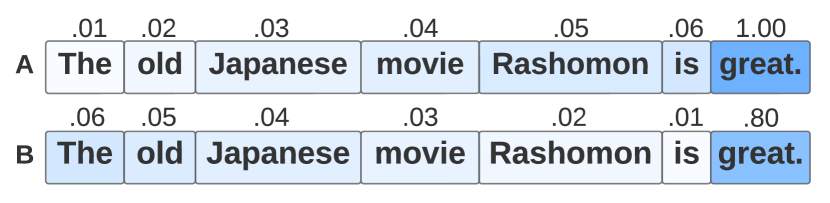
Figure 1: A toy example of sentiment classification illustrating the problems with Kendall-$\tau$. The corresponding agreement on the shown example is $k_{\tau}=-.43$ and $p_{r}=.99$. Token opacity indicates higher saliency score, i.e., token relevance, written out at the top of the token box. Each of the two explainability methods A and B outputs its saliency scores. The value of Kendall-$\tau$ is much lower than Pearson’s correlation, because the irrelevant tokens are perturbed, despite the fact that the tokens are correctly partitioned into more important and less important ones.

4.2 Regularizing Models

		$\tau_{k}$			$r_{p}$
		B	C	T	B	C	T
jwa	SUBJ	$.52$	$.48$	$\mathbf{.65}$†	$.66$	$.70$	$\mathbf{.88}$†
	SST	$.50$	$.67$	$\mathbf{.68}$	$.65$	$\mathbf{.90}$†	$.86$
	TREC	$.37$	$\mathbf{.77}$†	$.68$	$.52$	$\mathbf{.98}$†	$.93$
	IMDB	$.47$	$.52$	$\mathbf{.60}$†	$.72$	$.64$	$\mathbf{.80}$†
dbert	SUBJ	$.18$	$.28$	$\mathbf{.36}$†	$.31$	$.48$	$\mathbf{.57}$†
	SST	$.15$	$.15$	$\mathbf{.33}$†	$.28$	$.27$	$\mathbf{.60}$†
	TREC	$.18$	$.17$	$\mathbf{.28}$†	$.35$	$.34$	$\mathbf{.53}$†
	IMDB	$.18$	$.20$	$\mathbf{.24}$†	$.36$	$.42$	$\mathbf{.51}$†

Table 2: Average agreement over all pairs of saliency methods. We report agreement in terms of Kendall-$\tau$ ($k_{\tau}$) and Pearson-$r$ ($r_{p}$) from the last epoch for three model variants: B – base, C – conicity, and T – tying. Bold numbers indicate highest agreement among the three model flavors. Results are averages over $5$ runs with different seeds. We ran one-sided Wilcoxon signed-rank tests to check for statistical significance. Agreement values significantly higher ($p<.05$) than the other variants in two individual Wilcoxon tests are marked with a $\dagger$. We adjusted the $p$-values for family-wise error rate due to multiple tests using the Holm-Bonferroni method.

		Base	Conicity	Tying
dbert	SUBJ	$.93_{.01}$	$.90_{.02}$	$.93_{.00}$
	SST	$.83_{.00}$	$.83_{.01}$	$.82_{.01}$
	TREC	$.92_{.01}$	$.92_{.01}$	$.91_{.01}$
	IMDB	$.86_{.01}$	$.86_{.01}$	$.88_{.00}$
jwa	SUBJ	$.92_{.00}$	$.90_{.00}$	$.89_{.00}$
	SST	$.78_{.04}$	$.76_{.02}$	$.78_{.02}$
	TREC	$.89_{.02}$	$.86_{.01}$	$.89_{.01}$
	IMDB	$.89_{.00}$	$.88_{.00}$	$.86_{.00}$

Table 3: $F_{1}$ scores on test sets across datasets for dbert and jwa. We report the test results on epochs in which the model had the best performance on the validation set. Columns correspond to the base and regularized models. Numbers in subscript denote standard deviation on $5$ runs with different seeds.

Our next goal is to improve agreement between saliency methods through intervention in the training procedure, namely by applying regularization to promote disentanglement in the hidden space. In Table 2 we report correlation scores on the test splits of all datasets for regularized models (conicity, tying) and their unregularized variants (base). We notice that both regularization techniques have a positive effect on agreement across both correlation metrics, indicating that regularization techniques alleviate a deeper issue that also affects the interpretability of attention weights. In Table 3 we report $F_{1}$ scores on the test set for the regularized and unregularized models with the best performance on the validation split. We observe that regularized models generally perform comparably well to unregularized ones on downstream tasks, indicating that the improvement in the agreement does not come at a cost for downstream performance. When selecting regularized models, we choose ones with the strongest regularization scale hyperparameter that performs within $3$ $F_{1}$ points on the validation set compared to the unregularized model (cf. details in Section A.2).

5 The Cartography of Agreement

We have shown that by using a more appropriate correlation measure and applying regularization, the agreement of saliency methods increases significantly. In this section, we are interested in finding out the cause of increased agreement obtained through applying regularization – are there certain instance groups in the dataset that benefit the most, and if so, what changes in the representation space resulted in the increased agreement? We leverage methods from dataset cartography Swayamdipta et al. (2020) to distribute instances into easy-to-learn, hard-to-learn, and ambiguous categories based on their prediction confidence and variability. Concretely, if an instance exhibits low prediction variability and high prediction confidence between epochs, this implies that the model can quickly and accurately classify those instances, making them easy-to-learn. Instances that also exhibit low variability but low prediction confidence, align with the idea that the model is consistently unable to correctly classify them, making them hard-to-learn. Finally, instances that exhibit high variability and confidence close to the decision threshold indicate that the model is likely often changing its prediction between class labels for those instances, making them ambiguous. Since ambiguous instances are characterized by confidence near the prediction threshold, Swayamdipta et al. (2020) complement variability and confidence with another statistic introduced by Chang et al. (2017), namely closeness, defined as $c_{i}=p^{(i)}\cdot(1-p^{(i)})$, where $p^{(i)}$ is the average correct class probability of instance $x^{(i)}$ across all training epochs. A high closeness value denotes that the instance is consistently near the decision boundary, and thus is a good indicator of ambiguity within the model.

Intuitively, one would expect high agreement between saliency methods on instances that are easy to learn and low agreement otherwise. However, when computing how agreement distributes across instance groups, we find the converse is true. In unregularized models, we observe that easy-to-learn instances exhibit low average agreement, while ambiguous instances have a high average agreement. In Table 4, we report average agreement scores across all pairs of saliency methods on representative samples from each cartography group. We observe a clear distinction in agreement for both the base and regularized models, which is higher for ambiguous instances when compared to easy- and hard-to-learn instance groups. Furthermore, we can observe a consistently high increase in agreement when the models are regularized across all instance groups for all datasets, indicating that regularization techniques reduce representation entanglement.

One might wonder how the increase in agreement distributes across instances and dataset cartography attributes. In Figure 2, we visualize how the relationship between agreement and cartography attributes changes when the models are regularized. We observe that for the jwa model, all datasets exhibit a consistent and significant increase in agreement. Furthermore, we notice that for the dbert model, apart from increasing the agreement, regularization reduces the confidence of the model predictions and increases variability – indicating that it reduces the known problem of overconfidence present in pre-trained language models.

	Easy		Amb		Hard
	B	T	B	T	B	T
SUBJ	$.28$	$\mathbf{.52}$†	$.48$	$\mathbf{.74}$†	$.40$	$\mathbf{.57}$†
SST	$.24$	$\mathbf{.57}$†	$.36$	$\mathbf{.63}$†	$.30$	$\mathbf{.55}$†
TREC	$.33$	$\mathbf{.49}$†	$.50$	$\mathbf{.62}$†	$.32$	$\mathbf{.40}$†
IMDB	$.34$	$\mathbf{.48}$†	$.42$	$\mathbf{.59}$†	$.36$	$\mathbf{.51}$†

Table 4: Average agreement (Pearson-$r$) across saliency methods pairs per cartography groups. We select representative samples for each group based on the number of times a certain instance was classified correctly during training. We report average agreement for the unregularized model (B) and the one regularized by weight tying (T), with the numbers in bold indicating the higher agreement value among the two models. We averaged the results over $5$ runs. We ran one-sided Wilcoxon tests to check whether T is significantly better than B for a particular group. Significantly higher agreement values ($p<.05$) are marked with a $\dagger$.

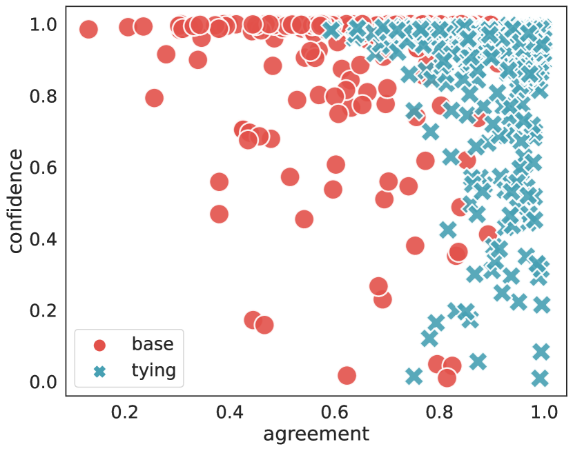
(a) jwa – SUBJ

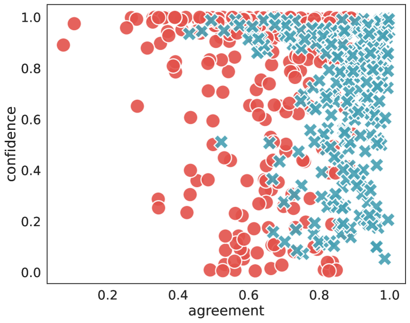
(b) jwa – SST

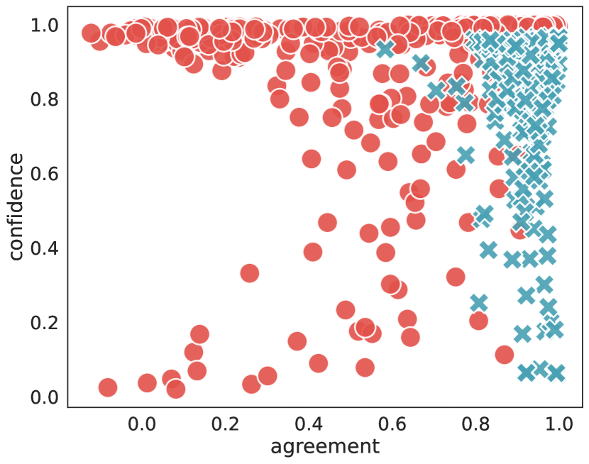
(c) jwa – TREC

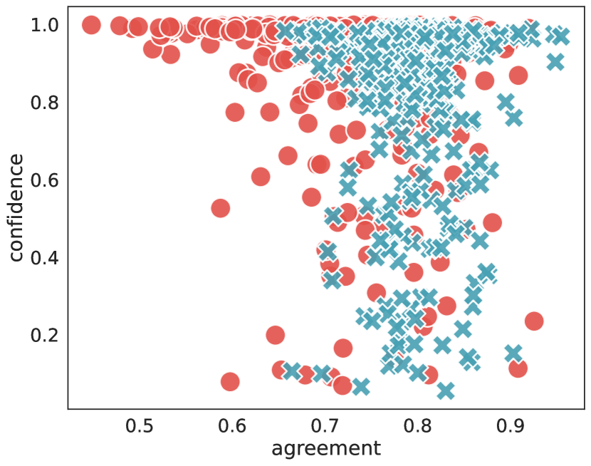
(d) jwa – IMDB

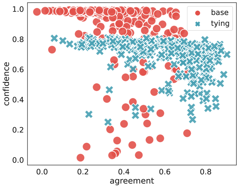
(e) dbert – SUBJ

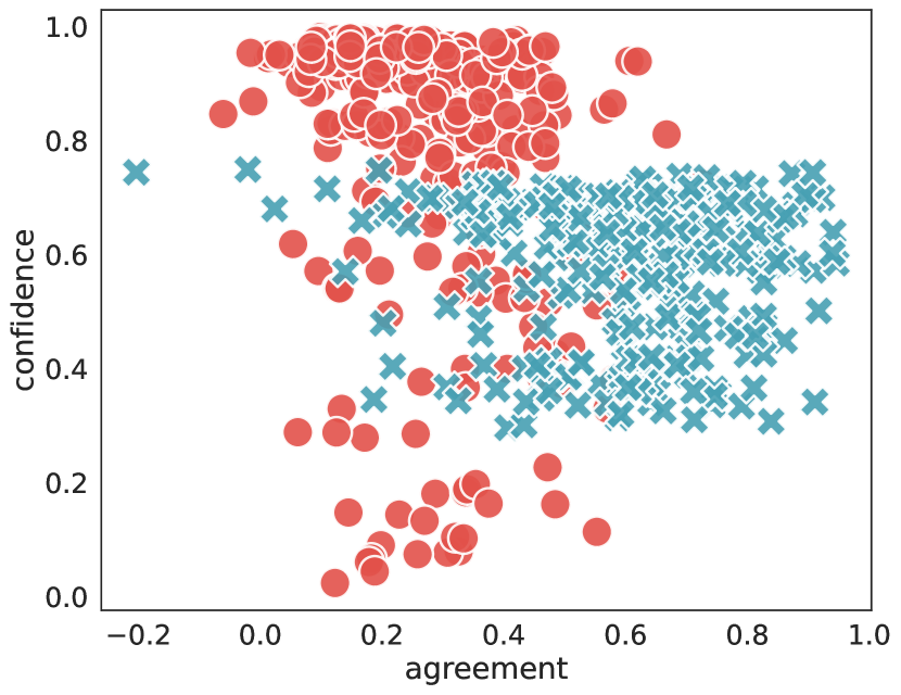
(f) dbert – SST

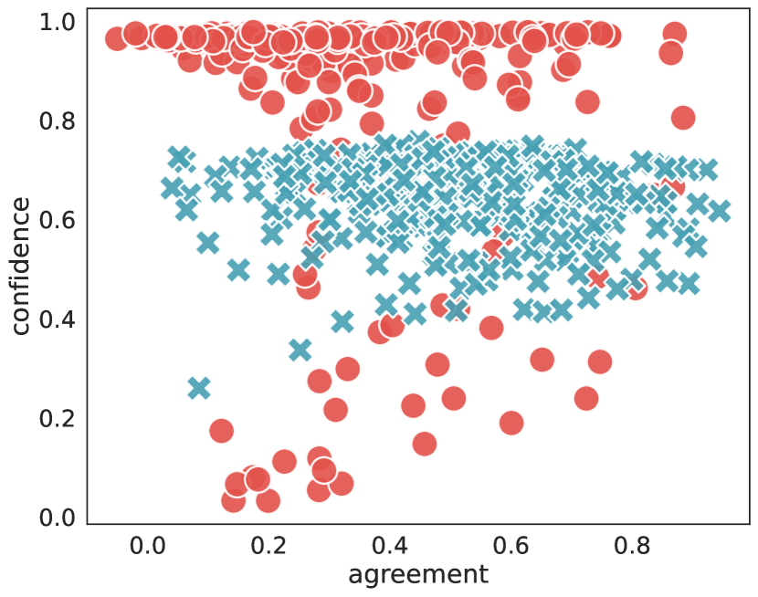
(g) dbert – TREC

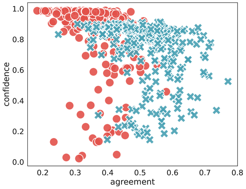
(h) dbert – IMDB

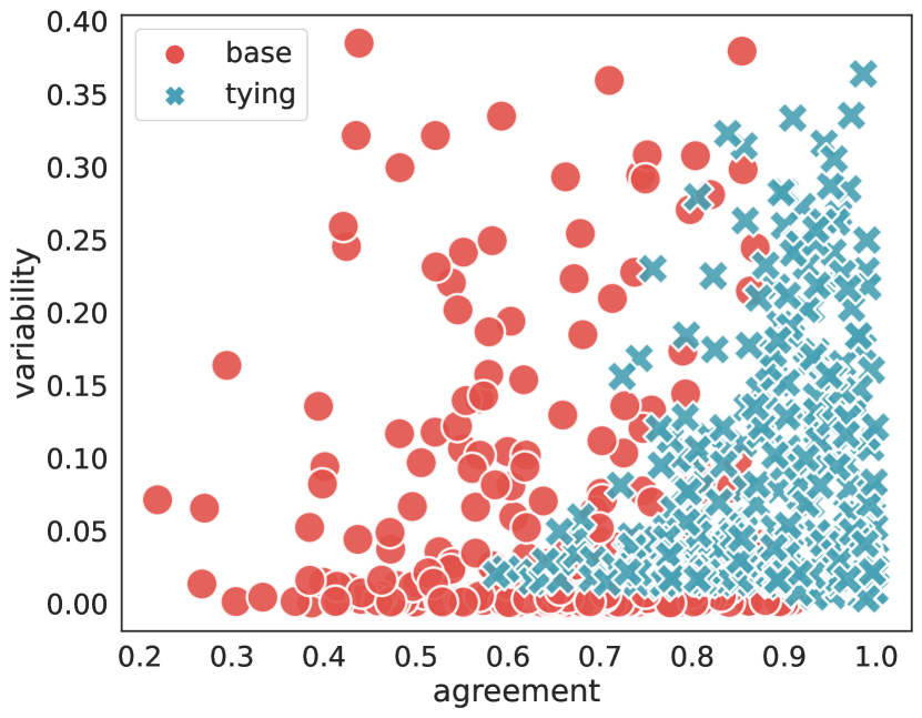
(i) jwa – SUBJ

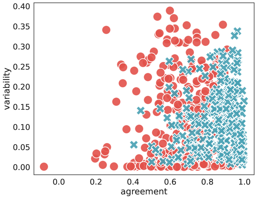
(j) jwa – SST

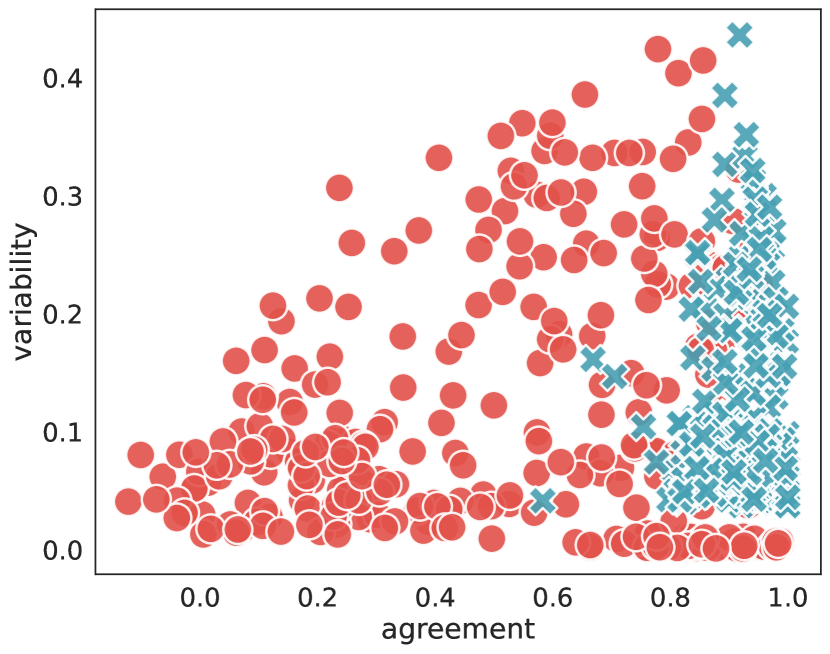
(k) jwa – TREC

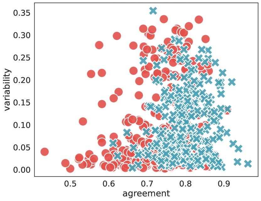
(l) jwa – IMDB

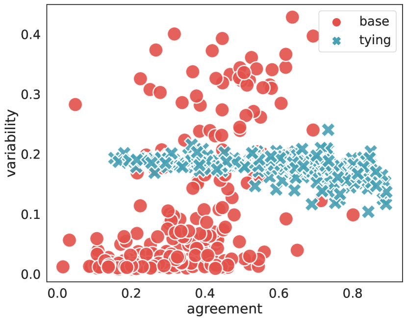
(m) dbert – SUBJ

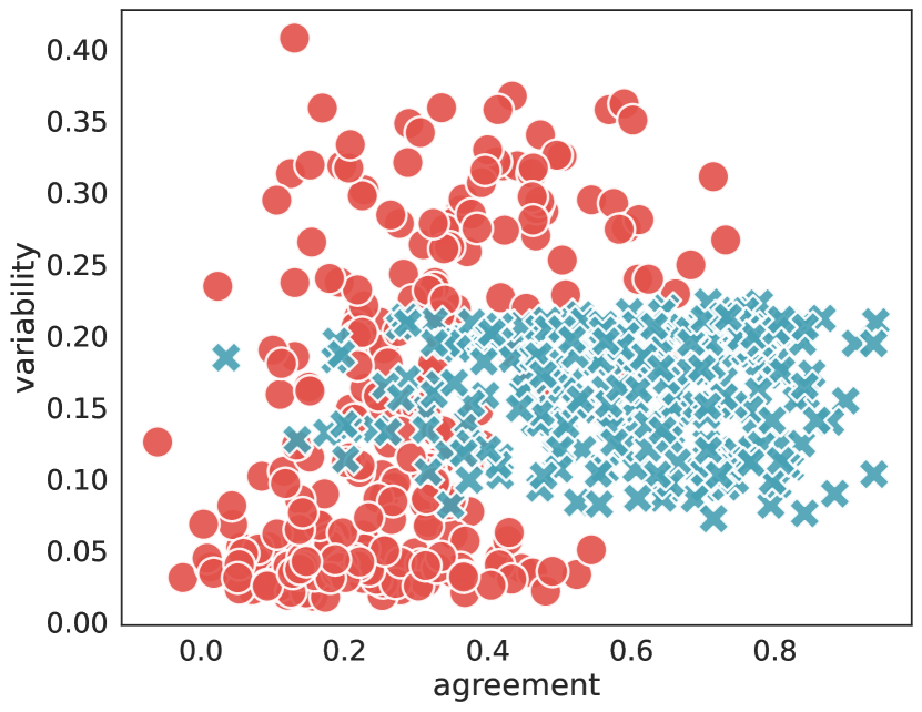
(n) dbert – SST

(o) dbert – TREC

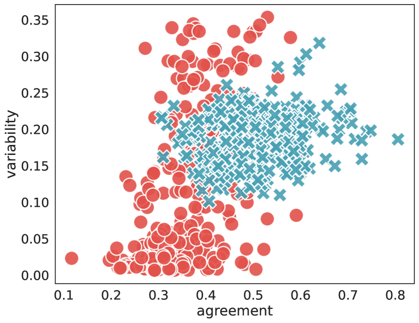
(p) dbert – IMDB

Figure 2: Relationship between agreement and cartography. Subfigures (a)–(h) and (i)–(p) show Pearson-$r$ agreement for each instance in the dataset with respect to confidence and variability, respectively. The red dots pertain to the unregularized model (base), and the blue crosses to the regularized model (tying).

5.1 The Curvature of Agreement

To better understand the cause of this distinction between various feature groups, we now analyze local curvature and density in the representation space. We are interested in: (1) how densely the instances are distributed in the representation space across cartography categories and (2) whether the local space around an instance is sharp or smooth. For both models and all instances, we obtain sequence representations $h$ used as inputs to the decoder. We estimate instance density as the average distance to the nearest instance in the dataset. We estimate local smoothness around an instance representation as the $L_{2}$ norm of the gradient of the hidden representation with respect to the input embeddings. If the gradient norm is high, the local space is sharp and minor perturbations can have a large effect on the prediction probability.

In Table 5, we report correlations between each of these two statistics and dataset cartography attributes. We observe that for the unregularized model, there is a significant negative correlation between confidence and both gradient norm and minimum distance to the nearest example, indicating that the local space around easy instances is smooth and densely populated. On the other hand, there is a high positive correlation between both closeness and variability and both gradient norm and minimum distance to the nearest example – indicating that the local space around ambiguous instances is sharp and sparsely populated. When we turn our attention to the regularized model, we observe that the correlation between the gradient norm and any of the cartography attributes vanishes, while the correlations between distance and the attributes are reduced in absolute value and their sign is flipped.

From these observations, we hypothesize that the cause of low agreement on easy-to-learn instances is the multitude of possible explanations as to why such an instance should be correctly classified. From the viewpoint of plausibility, this hypothesis is in line with the Rashomon effect Breiman (2001) which is about there often existing a multitude of adequate descriptions that end up with the same error rate, or in our case, prediction probability – however it should not apply to faithfulness, as a single model instance should adhere to a single explanation. However, due to a plethora of corroborating evidence for easy-to-learn instances, the representation space around them is smooth to such an extent that perturbations do not significantly affect the prediction probability, which in turn adversely affects gradient- and propagation-based explanation methods. The converse is true for ambiguous instances, where we hypothesize the model observes evidence for both classes and is unable to reach a confident decision. However, this difficulty in reaching a decision also causes saliency methods to have a precise definition of what the evidence is – as the local curvature is sharp, and any minor perturbation could significantly affect prediction probability. We believe that local curvature statistics could be used as a metric for measuring whether a trained model is better suited to analysis through explainability methods.

	Conf		Close		Var
	B	T	B	T	B	T
Grad norm	$-.39$	$-.02$	$.52$	$.05$	$.46$	$.06$
Min dist	$-.53$	$.25$	$.72$	$-.39$	$.64$	$.16$

Table 5: Correlations (Pearson-$r$) between local curvature statistics in the representation space and cartography attributes. We report average gradient norms (grad norm) of the hidden representation with respect to the input embeddings and average distance to the nearest instance (min dist). Columns correspond to the cartography attributes: conf – confidence, close – closeness, and var – confidence variance. We report the results for the base model (B) and the model regularized by tying (T). Results reported are averages over all datasets.

6 Conclusion

We analyzed two prototypical models from different families in jwa and dbert with the goal of finding out the cause of low agreement between saliency method interpretations. We first took a closer look at the previously used rank-order correlation metric and demonstrated that it is prone to exhibiting a high difference in agreement for small changes in importance scores. As an alternative, we used a linear correlation metric that is robust to small importance perturbations and demonstrated that it exhibits consistently higher agreement scores. Taking a step further, we applied two regularization techniques, tying and conicity, originally aimed at increasing faithfulness of attention explanations, with the hypothesis that the issue underpinning disagreements and unfaithfulness is the same – representation entanglement in the hidden space. We showed that regularization consistently and significantly improves agreement scores across all models and datasets with a minimal penalty for classification performance. Having demonstrated that it is possible to improve upon the low agreement scores, we attempted to offer intuition on which instance categories saliency methods agree the least and show that surprisingly, easy-to-learn instances are hard to agree on. Lastly, we offered insights into how the representation space morphs when regularization is applied and linked these findings with dataset cartography categories, paving the way for further work on understanding what properties of neural models affect interpretability.

Limitations

Our work has a number of important limitations that affect the conclusions we can draw from it. First and foremost, evaluating the faithfulness of model interpretations is problematic as we do not have ground truth annotations for token importances. Thus, when applying the agreement-as-evaluation paradigm, we implicitly assume that most saliency methods are close to the truth – an assumption that we cannot verify. However, every method of evaluating faithfulness has its own downsides. Token and representation erasure runs the risk of drawing conclusions from corrupted inputs that fall off the data manifold. We argue that while agreement-as-evaluation is far from an ideal way of evaluating faithfulness, it still increases credibility when used along with other techniques.

Secondly, our work is limited both with respect to the datasets and models considered. Specifically, we only evaluate one Transformer-based model from the masked language modeling family, and it is entirely possible that the findings do not generalize to models pre-trained on different tasks. Also, we only consider single sequence classification datasets – mainly due to the fact that the issues with the faithfulness of attention were most prevalent in those setups, which we assumed would be the same for agreement due to the same hypothesized underlying issue. We believe that tasks that require retention of token-level information in hidden states, such as sequence labeling and machine translation, would exhibit higher agreement overall, even without intervention through regularization. We leave this analysis for future work.

Appendix A Reproducibility

A.1 Experimental results

A.1.1 Setup

For both jwa and dbert, we use the same preprocessing pipeline on all four datasets. First, we filter out instances with fewer than three tokens to achieve stable agreement evaluation. Next, we lowercase the tokens, remove non-alphanumeric tokens, and truncate the sequence to $200$ tokens if the sequence length exceeds this threshold. We set the maximum vocabulary size to $20$k for models which do not leverage subword vocabularies.

A.1.2 Validation set performance

We report the validation set performance in Table 6.

A.1.3 Computing infrastructure

We conducted our experiments on $2\times$ AMD Ryzen Threadripper 3970X 32-Core Processors and $2\times$ NVIDIA GeForce RTX 3090 GPUs with $24$GB of RAM. We used PyTorch version $1.9.0$ and CUDA $11.4$.

A.1.4 Average runtime

Table 9 shows the average experiment runtime for each model across the datasets we used.

		Base	Conicity	Tying
dbert	SUBJ	$.94$	$.89$	$.94$
	SST	$.85$	$.85$	$.85$
	TREC	$.94$	$.89$	$.91$
	IMDB	$.90$	$.89$	$.89$
jwa	SUBJ	$.93$	$.90$	$.91$
	SST	$.82$	$.79$	$.81$
	TREC	$.91$	$.87$	$.89$
	IMDB	$.90$	$.87$	$.88$

Table 6: $F_{1}$ scores on validation sets across datasets for dbert and jwa. We average the results over $5$ runs with different seeds. The scores pertain to the same experiments as in Table 3, where we report test $F_{1}$ scores.

	jwa	dbert
SUBJ	$3.4$	$11.2$
SST	$2.7$	$8.9$
TREC	$1.2$	$3.7$
IMDB	$6.1$	$107.5$

Table 7: Experiment duration in minutes for both models across datasets. We report the average runtime over $5$ different runs.

A.1.5 Number of parameters

The jwa and dbert models that we used contained $1,714,951$ and $66,954,241$ trainable parameters, respectively.

A.2 Hyperparameter search

We used the following parameter grids for jwa: $[10^{-1},10^{-2},10^{-3},10^{-4},10^{-5},10^{-6}]$ for learning rate, and $[50,100,150,200]$ for the hidden state dimension. We yield best average results on validation sets across all datasets when the learning rate is set to $10^{-3}$ and the hidden size is set to $150$. For dbert, we find that the most robust initial learning rate on the four datasets is $2\times 10^{-5}$, among the options we explored $[5\times 10^{-4},10^{-4},10^{-5},2\times 10^{-5},5\times 10^{-5},10^{-6}]$. Additionally, we clip the gradients for both models such that the gradient norm $\leq 1$. We use the Adam Kingma and Ba (2015) optimizer for jwa and AdamW Loshchilov and Hutter (2017) for dbert. We run both models for $5$ epochs and repeat the experiments $5$ times with different seeds: $[1,2,3,4,5]$.

For regularization methods, we conducted a grid search with parameter grid $[0.1,0.3,0.5,1,5,10]$ for conicity and $[0.1,0.3,0.5,1,5,10,20]$ for tying. We select the models with the strongest regularization scale, which is within $3$ $F_{1}$ points from the unregularized model. Table 8 shows the selected values for each model across all datasets.

	jwa		dbert
	C	T	C	T
SUBJ	$1.$	$1.$	$5.$	$1.$
SST	$1.$	$0.5$	$0.1$	$0.5$
TREC	$1.$	$1.$	$0.1$	$0.3$
IMDB	$0.3$	$1.$	$1.$	$1.$

Table 8: Selected hyperparameter values for conicity (C) and tying (T).

	jwa	dbert
SUBJ	$3.4$	$11.2$
SST	$2.7$	$8.9$
TREC	$1.2$	$3.7$
IMDB	$6.1$	$107.5$

Table 9: Experiment duration in minutes for both models across datasets. We report the average runtime over $5$ different runs.

A.3 Dataset statistics

We report the number of instances per split for each dataset in Table 10. We note that all of the datasets we used contain predominantly texts in English.

	Train	Validation	Test	Total
SUBJ	$7,000$	$1,000$	$2,000$	$10,000$
SST	$6,819$	$868$	$1,810$	$9,497$
TREC	$1,987$	$159$	$486$	$2,632$
IMDB	$17,212$	$4,304$	$4,363$	$25,879$

Table 10: Number of instances in each split and the total number of instances in each dataset after we excluded too short examples (see section 3.1).

Appendix B Additional experiments

We show the full version of local curvature statistics in Table 11 (without averaging over datasets). In Figures 3, 4, 5, 6, 8, 7, 9 and 10 we plot correlation scores ($k_{\tau}$ and $p_{r}$) with standard deviation on the test splits. We include the results for all datasets across training epochs for regularized models (conicity, tying) when compared to their unregularized, base variants.

		Confidence		Ambiguity		Variability
		B	T	B	T	B	T
Grad norm	SUBJ	$-.37_{.00}$	$-.06_{.00}$	$.48_{.00}$	$.05_{.02}$	$.45_{.00}$	$.00_{.83}$
	SST	$-.40_{.00}$	$.02_{.34}$	$.58_{.00}$	$.08_{.00}$	$.42_{.00}$	$-.23_{.00}$
	TREC	$-.32_{.00}$	$.05_{.32}$	$.39_{.00}$	$-.12_{.01}$	$.38_{.00}$	$.18_{.00}$
	IMDB	$-.46_{.00}$	$-.11_{.00}$	$.61_{.00}$	$.17_{.00}$	$.60_{.00}$	$.30_{.00}$
Min dist	SUBJ	$-.59_{.00}$	$.01_{.70}$	$.79_{.00}$	$-.10_{.00}$	$.74_{.00}$	$.06_{.00}$
	SST	$-.45_{.00}$	$.30_{.00}$	$.70_{.00}$	$-.44_{.00}$	$.49_{.00}$	$.30_{.00}$
	TREC	$-.55_{.00}$	$.17_{.00}$	$.70_{.00}$	$-.26_{.00}$	$.68_{.00}$	$.25_{.00}$
	IMDB	$-.53_{.00}$	$.50_{.00}$	$.70_{.00}$	$-.74_{.00}$	$.64_{.00}$	$.04_{.00}$

Table 11: Correlations between local curvature statistics in the representation space and cartography attributes for each dataset. We use average gradient norms (grad norm) of the hidden representation with respect to the input embeddings and average distance to the nearest instance (min dist). The columns correspond to the cartography attributes. We report the results for the unregularized model (B) and the regularized one to which we applied tying (T). The values in the subscript denote the standard deviation.

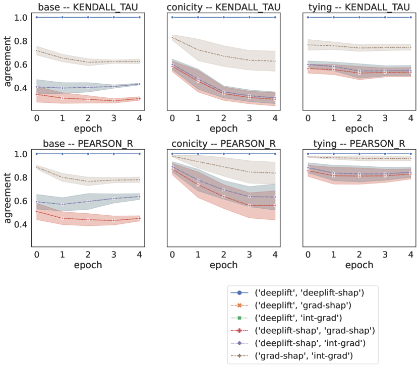
Figure 3: jwa – SUBJ

Figure 4: jwa – SST

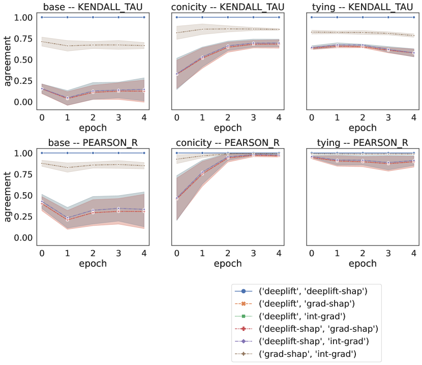
Figure 5: jwa – TREC

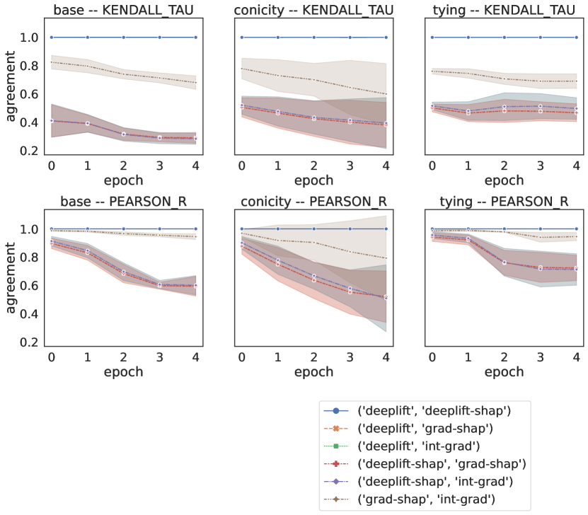
Figure 6: jwa – IMDB

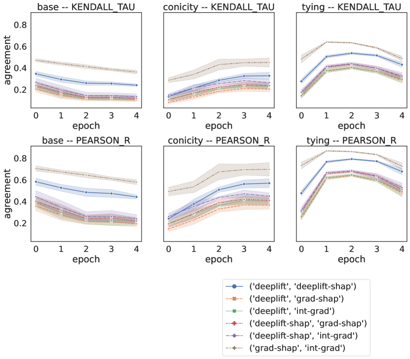
Figure 7: dbert – SUBJ

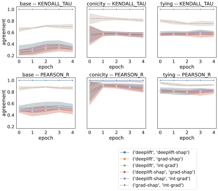
Figure 8: dbert – SST

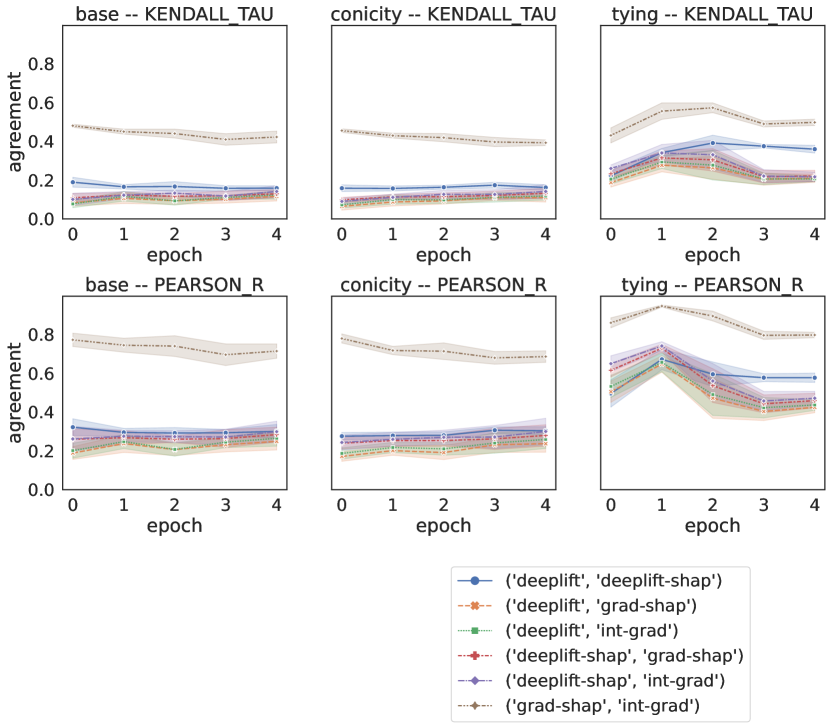
Figure 9: dbert – TREC

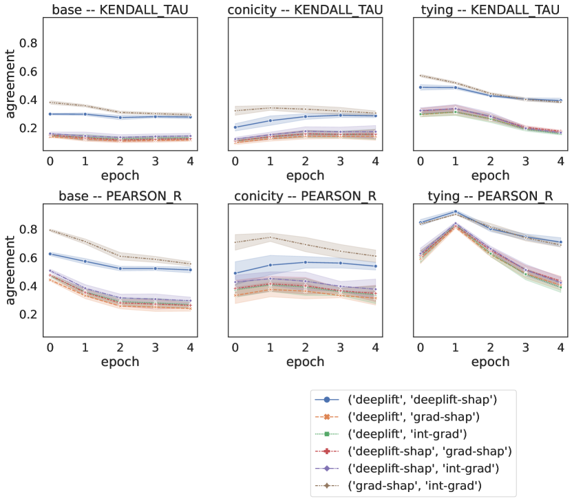
Figure 10: dbert – IMDB

References

- Abnar and Zuidema (2020) Samira Abnar and Willem Zuidema. 2020. Quantifying attention flow in transformers. In Proceedings of the 58th Annual Meeting of the Association for Computational Linguistics, pages 4190–4197.
- Atanasova et al. (2020) Pepa Atanasova, Jakob Grue Simonsen, Christina Lioma, and Isabelle Augenstein. 2020. A diagnostic study of explainability techniques for text classification. arXiv preprint arXiv:2009.13295.
- Bach et al. (2015) Sebastian Bach, Alexander Binder, Grégoire Montavon, Frederick Klauschen, Klaus-Robert Müller, and Wojciech Samek. 2015. On pixel-wise explanations for non-linear classifier decisions by layer-wise relevance propagation. PloS one, 10(7):e0130140.
- Bahdanau et al. (2014) Dzmitry Bahdanau, Kyunghyun Cho, and Yoshua Bengio. 2014. Neural machine translation by jointly learning to align and translate. arXiv preprint arXiv:1409.0473.
- Bastings et al. (2019) Jasmijn Bastings, Wilker Aziz, and Ivan Titov. 2019. Interpretable neural predictions with differentiable binary variables. arXiv preprint arXiv:1905.08160.
- Bastings et al. (2021) Jasmijn Bastings, Sebastian Ebert, Polina Zablotskaia, Anders Sandholm, and Katja Filippova. 2021. " will you find these shortcuts?" a protocol for evaluating the faithfulness of input salience methods for text classification. arXiv preprint arXiv:2111.07367.
- Bastings and Filippova (2020) Jasmijn Bastings and Katja Filippova. 2020. The elephant in the interpretability room: Why use attention as explanation when we have saliency methods? In Proceedings of the Third BlackboxNLP Workshop on Analyzing and Interpreting Neural Networks for NLP, pages 149–155.
- Breiman (2001) Leo Breiman. 2001. Statistical modeling: The two cultures (with comments and a rejoinder by the author). Statistical science, 16(3):199–231.
- Camburu et al. (2018) Oana-Maria Camburu, Tim Rocktäschel, Thomas Lukasiewicz, and Phil Blunsom. 2018. e-snli: Natural language inference with natural language explanations. Advances in Neural Information Processing Systems, 31.
- Caruana et al. (2015) Rich Caruana, Yin Lou, Johannes Gehrke, Paul Koch, Marc Sturm, and Noemie Elhadad. 2015. Intelligible models for healthcare: Predicting pneumonia risk and hospital 30-day readmission. In Proceedings of the 21th ACM SIGKDD international conference on knowledge discovery and data mining, pages 1721–1730.
- Chang et al. (2017) Haw-Shiuan Chang, Erik Learned-Miller, and Andrew McCallum. 2017. Active bias: Training more accurate neural networks by emphasizing high variance samples. In Advances in Neural Information Processing Systems, volume 30. Curran Associates, Inc.
- Croux and Dehon (2010) Christophe Croux and Catherine Dehon. 2010. Influence functions of the spearman and kendall correlation measures. Statistical methods & applications, 19(4):497–515.
- Denil et al. (2014) Misha Denil, Alban Demiraj, and Nando De Freitas. 2014. Extraction of salient sentences from labelled documents. arXiv preprint arXiv:1412.6815.
- Feng et al. (2018) Shi Feng, Eric Wallace, Alvin Grissom II, Mohit Iyyer, Pedro Rodriguez, and Jordan Boyd-Graber. 2018. Pathologies of neural models make interpretations difficult. In Proceedings of the 2018 Conference on Empirical Methods in Natural Language Processing, pages 3719–3728.
- Grath et al. (2018) Rory Mc Grath, Luca Costabello, Chan Le Van, Paul Sweeney, Farbod Kamiab, Zhao Shen, and Freddy Lecue. 2018. Interpretable credit application predictions with counterfactual explanations. arXiv preprint arXiv:1811.05245.
- Hooker et al. (2019) Sara Hooker, Dumitru Erhan, Pieter-Jan Kindermans, and Been Kim. 2019. A benchmark for interpretability methods in deep neural networks. Advances in neural information processing systems, 32.
- Jacovi and Goldberg (2020) Alon Jacovi and Yoav Goldberg. 2020. Towards faithfully interpretable NLP systems: How should we define and evaluate faithfulness? In Proceedings of the 58th Annual Meeting of the Association for Computational Linguistics, pages 4198–4205, Online. Association for Computational Linguistics.
- Jain and Wallace (2019) Sarthak Jain and Byron C Wallace. 2019. Attention is not explanation. In Proceedings of the 2019 Conference of the North American Chapter of the Association for Computational Linguistics: Human Language Technologies, Volume 1 (Long and Short Papers), pages 3543–3556.
- Jain et al. (2020) Sarthak Jain, Sarah Wiegreffe, Yuval Pinter, and Byron C Wallace. 2020. Learning to faithfully rationalize by construction. In Proceedings of the 58th Annual Meeting of the Association for Computational Linguistics, pages 4459–4473.
- Kehl and Kessler (2017) Danielle Leah Kehl and Samuel Ari Kessler. 2017. Algorithms in the criminal justice system: Assessing the use of risk assessments in sentencing.
- Kendall (1938) Maurice G Kendall. 1938. A new measure of rank correlation. Biometrika, 30(1/2):81–93.
- Kindermans et al. (2019) Pieter-Jan Kindermans, Sara Hooker, Julius Adebayo, Maximilian Alber, Kristof T Schütt, Sven Dähne, Dumitru Erhan, and Been Kim. 2019. The (un) reliability of saliency methods. In Explainable AI: Interpreting, Explaining and Visualizing Deep Learning, pages 267–280. Springer.
- Kingma and Ba (2015) Diederik P. Kingma and Jimmy Ba. 2015. Adam: A method for stochastic optimization. In 3rd International Conference on Learning Representations, ICLR 2015, San Diego, CA, USA, May 7-9, 2015, Conference Track Proceedings.
- Lei et al. (2016) Tao Lei, Regina Barzilay, and Tommi Jaakkola. 2016. Rationalizing neural predictions. In Proceedings of the 2016 Conference on Empirical Methods in Natural Language Processing, pages 107–117, Austin, Texas. Association for Computational Linguistics.
- Li et al. (2016) Jiwei Li, Will Monroe, and Dan Jurafsky. 2016. Understanding neural networks through representation erasure. arXiv preprint arXiv:1612.08220.
- Li and Roth (2002) Xin Li and Dan Roth. 2002. Learning question classifiers. In COLING 2002: The 19th International Conference on Computational Linguistics.
- Loshchilov and Hutter (2017) Ilya Loshchilov and Frank Hutter. 2017. Fixing weight decay regularization in adam. CoRR, abs/1711.05101.
- Lundberg and Lee (2016) Scott Lundberg and Su-In Lee. 2016. An unexpected unity among methods for interpreting model predictions. arXiv preprint arXiv:1611.07478.
- Maas et al. (2011) Andrew L. Maas, Raymond E. Daly, Peter T. Pham, Dan Huang, Andrew Y. Ng, and Christopher Potts. 2011. Learning word vectors for sentiment analysis. In Proceedings of the 49th Annual Meeting of the Association for Computational Linguistics: Human Language Technologies, pages 142–150, Portland, Oregon, USA. Association for Computational Linguistics.
- Madsen et al. (2021) Andreas Madsen, Nicholas Meade, Vaibhav Adlakha, and Siva Reddy. 2021. Evaluating the faithfulness of importance measures in nlp by recursively masking allegedly important tokens and retraining. arXiv preprint arXiv:2110.08412.
- Marasović et al. (2021) Ana Marasović, Iz Beltagy, Doug Downey, and Matthew E Peters. 2021. Few-shot self-rationalization with natural language prompts. arXiv preprint arXiv:2111.08284.
- Meister et al. (2021) Clara Meister, Stefan Lazov, Isabelle Augenstein, and Ryan Cotterell. 2021. Is sparse attention more interpretable? In Proceedings of the 59th Annual Meeting of the Association for Computational Linguistics and the 11th International Joint Conference on Natural Language Processing (Volume 2: Short Papers), pages 122–129.
- Mohankumar et al. (2020) Akash Kumar Mohankumar, Preksha Nema, Sharan Narasimhan, Mitesh M Khapra, Balaji Vasan Srinivasan, and Balaraman Ravindran. 2020. Towards transparent and explainable attention models. In Proceedings of the 58th Annual Meeting of the Association for Computational Linguistics, pages 4206–4216.
- Neely et al. (2021) Michael Neely, Stefan F Schouten, Maurits JR Bleeker, and Ana Lucic. 2021. Order in the court: Explainable ai methods prone to disagreement. arXiv preprint arXiv:2105.03287.
- Pang and Lee (2004) Bo Pang and Lillian Lee. 2004. A sentimental education: Sentiment analysis using subjectivity summarization based on minimum cuts. In Proceedings of the 42nd Annual Meeting of the Association for Computational Linguistics (ACL-04), pages 271–278, Barcelona, Spain.
- Pennington et al. (2014) Jeffrey Pennington, Richard Socher, and Christopher Manning. 2014. GloVe: Global vectors for word representation. In Proceedings of the 2014 Conference on Empirical Methods in Natural Language Processing (EMNLP), pages 1532–1543, Doha, Qatar. Association for Computational Linguistics.
- Ribeiro et al. (2016) Marco Tulio Ribeiro, Sameer Singh, and Carlos Guestrin. 2016. " why should i trust you?" explaining the predictions of any classifier. In Proceedings of the 22nd ACM SIGKDD international conference on knowledge discovery and data mining, pages 1135–1144.
- Sanh et al. (2019) Victor Sanh, Lysandre Debut, Julien Chaumond, and Thomas Wolf. 2019. Distilbert, a distilled version of BERT: smaller, faster, cheaper and lighter. CoRR, abs/1910.01108.
- Serrano and Smith (2019) Sofia Serrano and Noah A Smith. 2019. Is attention interpretable? In Proceedings of the 57th Annual Meeting of the Association for Computational Linguistics, pages 2931–2951.
- Shrikumar et al. (2017) Avanti Shrikumar, Peyton Greenside, and Anshul Kundaje. 2017. Learning important features through propagating activation differences. In International conference on machine learning, pages 3145–3153. PMLR.
- Sippy et al. (2020) Jacob Sippy, Gagan Bansal, and Daniel S Weld. 2020. Data staining: A method for comparing faithfulness of explainers. In Proceedings of ICML Workshop on Human Interpretability in Machine Learning.
- Socher et al. (2013) Richard Socher, John Bauer, Christopher D. Manning, and Andrew Y. Ng. 2013. Parsing with compositional vector grammars. In Proceedings of the 51st Annual Meeting of the Association for Computational Linguistics (Volume 1: Long Papers), pages 455–465, Sofia, Bulgaria. Association for Computational Linguistics.
- Sundararajan et al. (2017) Mukund Sundararajan, Ankur Taly, and Qiqi Yan. 2017. Axiomatic attribution for deep networks. In International Conference on Machine Learning, pages 3319–3328. PMLR.
- Swayamdipta et al. (2020) Swabha Swayamdipta, Roy Schwartz, Nicholas Lourie, Yizhong Wang, Hannaneh Hajishirzi, Noah A Smith, and Yejin Choi. 2020. Dataset cartography: Mapping and diagnosing datasets with training dynamics. arXiv preprint arXiv:2009.10795.
- Tutek and Šnajder (2020) Martin Tutek and Jan Šnajder. 2020. Staying true to your word:(how) can attention become explanation? In Proceedings of the 5th Workshop on Representation Learning for NLP, pages 131–142.
- Vaswani et al. (2017) Ashish Vaswani, Noam Shazeer, Niki Parmar, Jakob Uszkoreit, Llion Jones, Aidan N Gomez, Ł ukasz Kaiser, and Illia Polosukhin. 2017. Attention is all you need. In Advances in Neural Information Processing Systems, volume 30. Curran Associates, Inc.
- Wiegreffe and Pinter (2019) Sarah Wiegreffe and Yuval Pinter. 2019. Attention is not not explanation. In Proceedings of the 2019 Conference on Empirical Methods in Natural Language Processing and the 9th International Joint Conference on Natural Language Processing (EMNLP-IJCNLP), pages 11–20.