An environmental disturbance observer framework for autonomous ships

Abstract

This paper proposes a robust disturbance observer framework for maritime autonomous surface ships considering model and measurement uncertainties. The core contribution lies in a nonlinear disturbance observer, reconstructing the forces on a ship impacted by the environment, such as wind, waves, and sea currents. For this purpose, mappings are found that describe global exponentially stable error dynamics by assuming slow changes of disturbances. With the stability theory of Lyapunov, it is proven that the error converges exponentially into a ball, even if the disturbances are highly dynamic. Since measurements are affected by noise and physical models can be erroneous, the measurements are filtered through an unscented Kalman filter and propagated through the proposed observer to deal with noisy measurements and inaccurate models. To investigate the capability of this observer framework, the environmental disturbances are simulated at different severity levels. The results depict the simulation of a severe, worst-case scenario consisting of highly dynamic disturbances, intense measurement noise, and an unreliable ship model. It can be seen that the observer framework accurately reconstructs the forces on a ship impacted by the environment despite using a low measurement sampling rate, an erroneous model, and uncertain measurements.

InfoBox

1 Introduction

In the existing literature, several control concepts have been proposed for path following and collision avoidance for safe navigation. In this context, a precise perception of the environment is one of the essential elements of the ship’s situational awareness for safe sea operations. For example, sea currents might drift the ship away from the desired path, while the wind can affect the ship in its heading by creating a torque on the ship’s hull. If control algorithms are not considering these influences [1], safe and comfortable sea operations are not guaranteed. To accommodate these factors, some previous works consider the environmental impact. For instance, a disturbance observer-based control for dynamic positioning of ships is proposed in [2]. The proposal assumes a constant damping matrix and considers weak disturbances, such as in [3]. One of the few disturbance observers presented in [4] for tracking control considers model uncertainties. However, measurement uncertainties are neglected, and similar to the previously listed work, the damping matrix is oversimplified, making its use in real applications questionable. A backstepping control approach based on a disturbance observer and a neural network is presented in [5], where the ship stability concerning the roll motion is studied. Here, as well as in [6], only slowly varying disturbances are considered, while it is assumed that the measurements are entirely reliable. Despite ignoring model and measurement uncertainties, a widely used disturbance observer is presented in [7]. The proposal does not provide insight into the error dynamics of why it is difficult to guarantee sufficient adaptation speed regarding all observed disturbances. For this reason, synchronizing the error dynamics is a convenient way to supply controllers with consistent estimations. A detailed survey about the most popular disturbance observers is given in [8]. More recently, with the advancement of data-driven modeling, machine learning approaches for observing disturbances are coming up. A disturbance observer constructed by fusion of neural networks and minimal learning parameterization is proposed in [9] for robust dynamic positioning control under consideration of model and servo-system uncertainties. In [10], a data-driven adaptive disturbance observer for model-free trajectory tracking control of maritime autonomous surface ships is introduced. Common to all the data-driven approaches is that the models are trained with historical data and have a memory stack for online learning. Once again, most of such works are limited to scenarios with very weak disturbances. Since data-driven models are prone to overfitting and suffer from poor generalization outside the training scenarios, they are unfit to handling previously unseen severe and dynamic disturbances [11].

To summarise, none of the models demonstrate robust behavior under severe environmental conditions. Furthermore, none of the approaches consider measurement uncertainties, and the proposals disregard that measurements must be treated discretely. However, the sampling frequency of measurements is limited. Hence, this proposal tries to handle the previously described weaknesses in a novel observer framework by avoiding model simplifications but considering model and measurement uncertainties. To this end, the current work attempts to answer the following questions:

• Is it possible to observe the real disturbances accurately in situations where the sampling rate of the measurements is very low?

• Can we reconstruct the unknown disturbances despite measurement uncertainties?

• Is it possible to reconstruct the disturbances despite an unreliable model?

• Can a disturbance observer be designed where we can synchronize the adaptation speed of all observed disturbances?

To the best of our knowledge, none of the previous works have addressed all the research questions mentioned in a single study.

For a better comprehension of the work presented, the relevant theory, including the original contribution, is presented in Section 2. Section 3 presents all the details required to reproduce the results presented in the article. Results and their discussions are presented in Section 4 and finally, Section 5 concludes the current work.

2 Theory

In this section, we present a brief overview of the theory that is required for a better comprehension of the work presented. We begin by explaining the model of the ship used in Section 2.1 followed by a description of the unscented Kalman filter in Section 2.2. The original theoretical contribution of the work is presented in Sections 2.3 and 2.4.

2.1 Model

Considering the ship’s coordinates $\bm{\eta}=[x_{s},y_{s},\psi]^{\top}$, where $x_{s}$ and $y_{s}$ describes the ship’s position with regard to the global coordinates $[x,y]^{\top}$, and $\psi$ is the ship’s heading. Furthermore, the velocities are denoted as $\bm{\nu}=[u,v,r]^{\top}$, where $u$ is the surge, $v$ describes the sway, and $r$ characterizes the rotational speed regarding yaw. With these relations, the kinematics of a ship can be expressed by

$$\bm{\dot{\eta}}=\bm{R}_{\mathrm{rot}}(\psi)\bm{\nu},$$ (1)

where $\bm{R}_{\mathrm{rot}}(\psi)$ denotes the rotational matrix, given by

$$\bm{R}_{\mathrm{rot}}(\psi)=\begin{bmatrix}\mathrm{cos}(\psi)&&-\mathrm{sin}(\psi)&&0\\ \mathrm{sin}(\psi)&&\mathrm{cos}(\psi)&&0\\ 0&&0&&1\end{bmatrix}.$$ (2)

Fig. 1 depicts the relations between the different ship states.

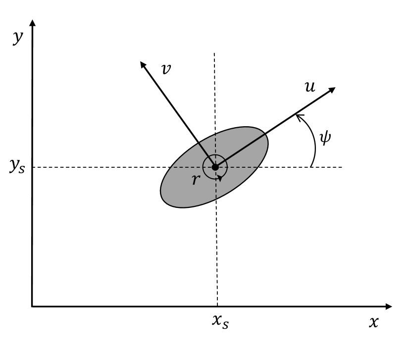
Fig. 1: Kinematics of a ship

The dynamics of a ship can be expressed as

$$\bm{M}\bm{\dot{\nu}}+\bm{D}(\bm{\nu})\bm{\nu}+\bm{C}(\bm{\nu})\bm{\nu}=\bm{\tau}+\bm{\tau_{d}},$$ (3)

where $\bm{M}$ denotes the mass matrix, $\bm{D}(\bm{\nu})$ characterizes the nonlinear damping matrix, $\bm{C}(\bm{\nu})$ describes the Coriolis matrix, $\bm{\tau}$ is the control input, and $\bm{\tau}_{d}$ are all the environmental disturbances. Therefore,

$$\bm{\tau_{d}}=\bm{\tau}_{\mathrm{wind}}+\bm{\tau}_{\mathrm{wave}}+\bm{\tau}_{\mathrm{current}},$$ (4)

which implies that the disturbances are specified as the sum of forces induced by wind, waves, and sea currents. Rewriting the dynamical expression in state space representation leads to

$$\bm{\dot{\nu}}=\bm{M}^{-1}\left(-\bm{D}(\bm{\nu})\bm{\nu}-\bm{C}(\bm{\nu})\bm{\nu}+\bm{\tau}+\bm{\tau_{d}}\right).$$ (5)

It is assumed that the mass matrix is symmetric and positive definite. Furthermore, the mass matrix has constant entries, defined as

$$\bm{M}=\begin{bmatrix}m_{11}&&0&&0\\ 0&&m_{22}&&m_{23}\\ 0&&m_{32}&&m_{33}\end{bmatrix},$$ (6)

since the mass is not dependent on the system states $\bm{\nu}$. Based on later derivations, the entries of the inverted mass matrix are denoted as

$$\bm{M}^{-1}=\begin{bmatrix}\kappa_{11}&&0&&0\\ 0&&\kappa_{22}&&\kappa_{23}\\ 0&&\kappa_{32}&&\kappa_{33}\end{bmatrix}.$$ (7)

Lemma 1

If the matrix $\bm{M}$ is symmetric and invertible, its inverse $\bm{M}^{-1}$ is likewise symmetric, since $(\bm{M}^{-1})^{\top}=\leavevmode\nobreak\ (\bm{M}^{\top})^{-1}$. Since the entries of the mass matrix are positive, $\bm{M}$ is positive definite, and thus invertible.

Moreover, it is assumed that the damping matrix is symmetric, and the Coriolis matrix is skew-symmetric such as in [12], given by

$$\bm{D}(\bm{\nu}) =\begin{bmatrix}d_{11}(\bm{\nu})&&0&&0\\ 0&&d_{22}(\bm{\nu})&&d_{23}(\bm{\nu})\\ 0&&d_{32}(\bm{\nu})&&d_{33}(\bm{\nu})\end{bmatrix},$$ (8)

$$\bm{C}(\bm{\nu}) =\begin{bmatrix}0&&0&&c_{13}(\bm{\nu})\\ 0&&0&&c_{23}(\bm{\nu})\\ c_{31}(\bm{\nu})&&c_{32}(\bm{\nu})&&0\end{bmatrix}.$$ (9)

The entries of the matrices are defined as

$$d_{11}(\bm{\nu}) =-X_{u}-X_{|u|u}-X_{uuu}u^{2},$$ (10a)

$$d_{22}(\bm{\nu}) =-Y_{v}-Y_{|v|v}-Y_{|r|v}|r|-Y_{vvv}v^{2},$$ (10b)

$$d_{23}(\bm{\nu}) =-Y_{r}-Y_{|v|r}|v|-Y_{|r|r}|r|,$$ (10c)

$$d_{32}(\bm{\nu}) =-N_{v}-N_{|v|v}|v|-N_{|r|v}|r|,$$ (10d)

$$d_{33}(\bm{\nu}) =-N_{r}-N_{|v|r}|v|-N_{|r|r}|r|-N_{rrr}r^{2},$$ (10e)

and

$$c_{13}(\bm{\nu}) =-m_{22}v-m_{23}r,$$ (11a)

$$c_{23}(\bm{\nu}) =m_{11}u,$$ (11b)

$$c_{31}(\bm{\nu}) =-c_{13}(\bm{\nu}),$$ (11c)

$$c_{32}(\bm{\nu}) =-c_{23}(\bm{\nu}),$$ (11d)

causing highly nonlinear model dynamics, where $X_{u}$, $X_{|u|u}$, $X_{uuu}$, $Y_{v}$, $Y_{|v|v}$, $Y_{|r|v}$, $Y_{vvv}$, $Y_{r}$, $Y_{|v|r}$, $Y_{|r|r}$, $N_{v}$, $N_{|v|v}$, $N_{|r|v}$, $N_{r}$, $N_{|v|r}$, $N_{|r|r}$, and $N_{rrr}$ are hydrodynamic parameters.

2.2 Unscented Kalman Filter

The unscented Kalman filter (UKF), proposed in [13], is proved to be a very powerful tool for state estimation of nonlinear systems with measurement noise and model uncertainty. Considering the time-discrete nonlinear dynamical system

$$\bm{\mathrm{x}}_{k+1} =\bm{f}(\bm{\mathrm{x}}_{k},\bm{\mathrm{w}}_{k}),$$ (12)

$$\bm{\mathrm{y}}_{k} =\bm{g}(\bm{\mathrm{x}}_{k},\bm{\mathrm{n}}_{k}),$$ (13)

where $\bm{f}$ and $\bm{g}$ are non-linear functions, $\bm{\mathrm{x}}_{k}$ describes the model states, and $\bm{\mathrm{y}}_{k}$ characterizes the measurement model at timestep $k$. The model and measurement uncertainties are modeled as Gaussian noise with zero mean. Hence, they are described by

$$\bm{\mathrm{w}}_{k}\sim\mathcal{N}(\bm{0},\bm{Q}_{k}),$$ (14)

$$\bm{\mathrm{n}}_{k}\sim\mathcal{N}(\bm{0},\bm{R}_{k}),$$ (15)

where $\bm{Q}_{k}$ and $\bm{R}_{k}$ specify the covariance matrix of the model and measurement uncertainties, respectively.
The main idea of the UKF is to use sigma points distributed symmetrically in the area of the mean and gate them through the nonlinear functions. Assume the states $\bm{\mathrm{x}}\in\mathbb{R}^{L}$ have the estimated mean $\bm{\mathrm{\hat{x}}}$ and covariance $\bm{P}$, the sigma points of the entire sigma point matrix $\bm{\mathcal{X}}\in\mathbb{R}^{L\times(2L+1)}$ are generated by

$$\bm{\mathcal{X}}_{0} =\bm{\mathrm{\hat{x}}},$$ (16a)

$$\bm{\mathcal{X}}_{i} =\bm{\mathrm{\hat{x}}}+\left(\sqrt{(L+\lambda)}\bm{P}\right)_{i},\ \ \ \ \ \ i=1,...,L,$$ (16b)

$$\bm{\mathcal{X}}_{i} =\bm{\mathrm{\hat{x}}}-\left(\sqrt{(L+\lambda)}\bm{P}\right)_{i-L},\ \ \ i=L+1,...,2L,$$ (16c)

where $\lambda=\alpha^{2}(L+\kappa)-L$. The tuning parameter $\alpha$ describes the spread of the sigma points, usually set to $\alpha=10^{-3}$, and $\kappa$ is a secondary tuning parameter, usually set to $\kappa=0$. The weights of each sigma point for calculating the means and covariances are defined as

$$W^{m}_{0}=\frac{\lambda}{L+\lambda},$$ (17)

$$W^{c}_{0}=\frac{\lambda}{L+\lambda}+(1-\alpha^{2}+\beta),$$ (18)

$$W^{m}_{i}=W^{c}_{i}=\frac{1}{2(L+\lambda)},\ \ \ i=1,...,2L,$$ (19)

where $\beta$ is a tuning parameter, which is usually set to $\beta=2$ for Gaussian distributions.

Prediction step
Calculate $\bm{\mathcal{X}}$ according to (16a)-(16c). Afterwards compute the following relations:

$$\bm{\check{\mathrm{x}}}=\sum_{i=0}^{2L}W^{m}_{i}\bm{f}(\bm{\mathcal{X}}_{i})$$ (20)

$$\bm{\check{\mathrm{y}}}=\sum_{i=0}^{2L}W^{m}_{i}\bm{g}(\bm{\mathcal{X}}_{i})$$ (21)

$$\bm{P}_{x}=\sum_{i=0}^{2L}W^{c}_{i}\left(\bm{f}(\bm{\mathcal{X}}_{i})-\bm{\check{\mathrm{x}}}\right)\left(\bm{f}(\bm{\mathcal{X}}_{i})-\bm{\check{\mathrm{x}}}\right)^{\top}$$ (22)

$$\bm{P}_{y}=\sum_{i=0}^{2L}W^{c}_{i}\left(\bm{g}(\bm{\mathcal{X}}_{i})-\bm{\check{\mathrm{y}}}\right)\left(\bm{g}(\bm{\mathcal{X}}_{i})-\bm{\check{\mathrm{y}}}\right)^{\top}$$ (23)

$$\bm{P}_{xy}=\sum_{i=0}^{2L}W^{c}_{i}\left(\bm{f}(\bm{\mathcal{X}}_{i})-\bm{\check{\mathrm{x}}}\right)\left(\bm{g}(\bm{\mathcal{X}}_{i})-\bm{\check{\mathrm{y}}}\right)^{\top}$$ (24)

Correction step

$$\bm{K}=\bm{P}_{xy}\bm{P}_{y}^{-1}$$ (25)

$$\bm{\mathrm{\hat{x}}}=\bm{\check{\mathrm{x}}}+\bm{K}(\bm{\mathrm{y}}-\bm{\check{\mathrm{y}}})$$ (26)

$$\bm{P}=\bm{P}_{x}-\bm{K}\bm{P}_{y}\bm{P}_{x}$$ (27)

Here, $\bm{\check{\mathrm{x}}}$ and $\bm{\check{\mathrm{y}}}$ are the predictions of the states and measurements, respectively, calculated by gating the sigma points $\bm{\mathcal{X}}$ through the nonlinear functions. The covariance matrices $\bm{P}_{x}$, $\bm{P}_{y}$, and the cross-covariance matrix $\bm{P}_{xy}$ are used for computing the updated covariance matrix $\bm{P}$ and the Kalman gain matrix $\bm{K}$. Hence, the Kalman gain matrix characterizes the trustworthiness of the predicted states $\bm{\check{\mathrm{x}}}$. If $\bm{K}$ has small values, the predictions are well-performing. Otherwise, the measurements $\bm{\mathrm{y}}$ are weighted stronger to correct the prediction inaccuracy. As a result, the estimations $\bm{\mathrm{\hat{x}}}$ result in a smoothed version of the measurements $\bm{\mathrm{x}}_{m}$.

2.3 Disturbance Observer Design

In the following, the original theoretical contribution of this article is explained. Two assumptions are made to formulate the disturbance observer.

Assumptions:

• It is assumed that the ship’s velocities $\bm{\nu}$ are measured. However, the measurements are expected to have uncertainties, described in more detail in section 2.4.

• It is assumed that the disturbances change slowly such that $\bm{\dot{\tau}_{d}}\approx\bm{0}$ holds for short time intervals.

To design the dynamical observer, we define the following relations

$$\bm{\hat{\tau}_{d}} =\bm{\zeta}+\bm{\mu}(\bm{\nu}),$$ (28)

$$\bm{\dot{\zeta}} =\bm{h}(\bm{\nu},\bm{\hat{\tau}_{d}}),$$ (29)

where the estimation of the disturbances $\bm{\hat{\tau}_{d}}$ is defined as the sum of an observer variable $\bm{\zeta}$ and an unknown mapping $\bm{\mu}(\bm{\nu})$. Hence, the error of the observer is defined as

$$\bm{z}=\bm{\tau_{d}}-\bm{\zeta}-\bm{\mu}(\bm{\nu}).$$ (30)

The dynamics of the observer variable are defined as an unknown mapping $\bm{h}(\bm{\nu},\bm{\hat{\tau}_{d}})$. Therefore, the goal is to find the mappings $\bm{\mu}(\bm{\nu})$ and $\bm{h}(\bm{\nu},\bm{\hat{\tau}_{d}})$, such that the estimation $\bm{\hat{\tau}_{d}}$ has a globally, asymptotically stable equilibrium at $\bm{z}=\bm{0}$, and converges to the manifold

$$\bm{\mathcal{M}}=\left\{(\bm{\nu},\bm{\zeta})\in\mathbb{R}^{3}\times\mathbb{R}^{3}:\bm{\tau_{d}}-\bm{\zeta}-\bm{\mu}(\bm{\nu})=\bm{0}\right\}.$$ (31)

The error dynamics are obtained by the time derivative of (30), yielding

$$\bm{\dot{z}}=\underbrace{\bm{\dot{\tau}_{d}}}_{\approx\bm{0}}-\bm{\dot{\zeta}}-\frac{\partial\bm{\mu}}{\partial\bm{\nu}}\dot{\bm{\nu}},$$ (32)

which leads to

$$\bm{\dot{z}}=-\bm{h}(\bm{\nu},\bm{\hat{\tau}_{d}})-\frac{\partial\bm{\mu}}{\partial\bm{\nu}}\bm{M}^{-1}\left(\left(-\bm{D}(\bm{\nu})-\bm{C}(\bm{\nu})\right)+\bm{\tau}+\bm{\tau_{d}}\right).$$ (33)

Remark 1

Since the error dynamics are described by (33), $\bm{\mu}(\bm{\nu})$ must be differentiable with respect to $\bm{\nu}$.

To find suitable error dynamics, we define $\bm{h}(\bm{\nu},\bm{\hat{\tau}_{d}})$ as

$$\bm{h}(\bm{\nu},\bm{\hat{\tau}_{d}})=-\frac{\partial\bm{\mu}}{\partial\bm{\nu}}\bm{M}^{-1}\left(\left(-\bm{D}(\bm{\nu})-\bm{C}(\bm{\nu})\right)+\bm{\tau}+\bm{\hat{\tau}_{d}}\right),$$ (34)

such that the error dynamics are given by

$$\bm{\dot{z}}=-\frac{\partial\bm{\mu}}{\partial\bm{\nu}}\bm{M}^{-1}(\bm{\tau_{d}}-\bm{\hat{\tau}_{d}})=-\frac{\partial\bm{\mu}}{\partial\bm{\nu}}\bm{M}^{-1}\bm{z}.$$ (35)

Generally, the observer dynamics $\bm{\dot{\zeta}}=\bm{h}(\bm{\nu},\bm{\hat{\tau}_{d}})$ are formulated as

$$\bm{\dot{\zeta}}=-\frac{\partial\bm{\mu}(\bm{\nu})}{\partial\bm{\nu}}\bm{\dot{\nu}}(\bm{\tau_{d}}=\bm{\zeta}+\bm{\mu}(\bm{\nu})),$$ (36)

where the partial derivative $\frac{\partial\bm{\mu}(\bm{\nu})}{\partial\bm{\nu}}$ is given by

$$\frac{\partial\bm{\mu}(\bm{\nu})}{\partial\bm{\nu}}=\begin{bmatrix}\frac{\partial\mu_{1}}{\partial u}&&\frac{\partial\mu_{1}}{\partial v}&&\frac{\partial\mu_{1}}{\partial r}\\[6.0pt] \frac{\partial\mu_{2}}{\partial u}&&\frac{\partial\mu_{2}}{\partial v}&&\frac{\partial\mu_{2}}{\partial r}\\[6.0pt] \frac{\partial\mu_{3}}{\partial u}&&\frac{\partial\mu_{3}}{\partial v}&&\frac{\partial\mu_{3}}{\partial r}\end{bmatrix}.$$ (37)

Considering the error dynamics, and the system dynamics, it is reasonable to define

$$\bm{\mu}(\bm{\nu})=\begin{bmatrix}\mu_{1}(u)\\[6.0pt] \mu_{2}(v,r)\\[6.0pt] \mu_{3}(v,r)\end{bmatrix},$$ (38)

such that

$$\frac{\partial\bm{\mu}(\bm{\nu})}{\partial\bm{\nu}}=\begin{bmatrix}\frac{\partial\mu_{1}}{\partial u}&&0&&0\\[6.0pt] 0&&\frac{\partial\mu_{2}}{\partial v}&&\frac{\partial\mu_{2}}{\partial r}\\[6.0pt] 0&&\frac{\partial\mu_{3}}{\partial v}&&\frac{\partial\mu_{3}}{\partial r}\end{bmatrix}.$$ (39)

With these definitions, the error dynamics yield

$$\leavevmode\resizebox{422.77661pt}{25.72377pt}{$\bm{\dot{z}}=-\begin{bmatrix}\frac{\partial\mu_{1}}{\partial u}\kappa_{11}&&0&&0\\[6.0pt] 0&&\frac{\partial\mu_{2}}{\partial v}\kappa_{22}+\frac{\partial\mu_{2}}{\partial r}\kappa_{32}&&\frac{\partial\mu_{2}}{\partial v}\kappa_{23}+\frac{\partial\mu_{2}}{\partial r}\kappa_{33}\\[6.0pt] 0&&\frac{\partial\mu_{3}}{\partial v}\kappa_{22}+\frac{\partial\mu_{3}}{\partial r}\kappa_{32}&&\frac{\partial\mu_{3}}{\partial v}\kappa_{23}+\frac{\partial\mu_{3}}{\partial r}\kappa_{33}\end{bmatrix}\begin{bmatrix}z_{1}\\ z_{2}\\ z_{3}\end{bmatrix}$}.$$ (40)

Regarding $z_{1}$, it is evident that the error dynamics are exponentially stable for every $\mu_{1}(u)$, which satisfies

$$\frac{\partial\mu_{1}}{\partial u}\kappa_{11}>0.$$ (41)

To guarantee stable error dynamics concerning $z_{2}$ and $z_{3}$, we define the following conditions.

$$\textbf{C1:}\ \ \ \ \ \ \ \ \ \ \ \ \frac{\partial\mu_{2}}{\partial v}\kappa_{23}+\frac{\partial\mu_{2}}{\partial r}\kappa_{33}\stackrel{{\scriptstyle!}}{{=}}0$$ (42)

$$\textbf{C2:}\ \ \ \ \ \ \ \ \ \ \ \ \frac{\partial\mu_{2}}{\partial v}\kappa_{22}+\frac{\partial\mu_{2}}{\partial r}\kappa_{32}\stackrel{{\scriptstyle!}}{{>}}0$$ (43)

$$\textbf{C3:}\ \ \ \ \ \ \ \ \ \ \ \ \frac{\partial\mu_{3}}{\partial v}\kappa_{22}+\frac{\partial\mu_{3}}{\partial r}\kappa_{32}\stackrel{{\scriptstyle!}}{{=}}0$$ (44)

$$\textbf{C4:}\ \ \ \ \ \ \ \ \ \ \ \ \frac{\partial\mu_{3}}{\partial v}\kappa_{23}+\frac{\partial\mu_{3}}{\partial r}\kappa_{33}\stackrel{{\scriptstyle!}}{{>}}0$$ (45)

Here, C1 and C2 guarantee stable error dynamics with regard to $z_{2}$, while C3 and C4 ensure stable error dynamics concerning $z_{3}$. Since C1 and C3 are stronger conditions, we initially define

$$\mu_{2}(v,r)=\Gamma_{2}\left(\frac{1}{\kappa_{22}}v-\frac{\kappa_{23}}{\kappa_{22}\kappa_{33}}r\right),$$ (46)

$$\mu_{3}(v,r)=\Gamma_{3}\left(\frac{1}{\kappa_{33}}r-\frac{\kappa_{32}}{\kappa_{22}\kappa_{33}}v\right),$$ (47)

where $\Gamma_{2}$ and $\Gamma_{3}$ are adaptive gains. With these relations, C1 and C3 hold. Consequential, C2 and C4 lead to

$$\Gamma_{2}\left(1-\frac{\kappa_{23}\kappa_{32}}{\kappa_{22}\kappa_{33}}\right)\stackrel{{\scriptstyle!}}{{>}}0,$$ (48)

$$\Gamma_{3}\left(1-\frac{\kappa_{23}\kappa_{32}}{\kappa_{22}\kappa_{33}}\right)\stackrel{{\scriptstyle!}}{{>}}0.$$ (49)

Hence, we must consider three cases.

Case 1: $\kappa_{23}\kappa_{32}<\kappa_{22}\kappa_{33}$
In practice, the entries of the secondary diagonal of the mass matrix are usually much smaller than the diagonal. Hence, the absolute values of $\kappa_{23}$ and $\kappa_{32}$ are also much smaller than $\kappa_{22}$ and $\kappa_{33}$. In this case C2 and C4 are satisfied if $\Gamma_{2}>0$ and $\Gamma_{3}>0$.

Case 2: $\kappa_{23}\kappa_{32}>\kappa_{22}\kappa_{33}$
This case is usually not true. However, if this unrealistic scenario holds, C2 and C4 are satisfied if $\Gamma_{2}<0$ and $\Gamma_{3}<0$.

Case 3: $\kappa_{23}\kappa_{32}=\kappa_{22}\kappa_{33}$
In this case, the observer will not adapt. However, this case is usually neglectable since this case is also unrealistic.

Remark 2

Since all entries of the mass matrix are positive, $\frac{\kappa_{23}\kappa_{32}}{\kappa_{22}\kappa_{33}}$ is always positive.

For future considerations, we regard the first case. To satisfy (41) and to synchronize the error dynamics, we define

$$\mu_{1}(u)=\Gamma_{1}\frac{1}{\kappa_{11}}u\left(1-\frac{\kappa_{23}\kappa_{32}}{\kappa_{22}\kappa_{33}}\right).$$ (50)

The previous case study also holds for (50) and the corresponding error dynamics of $z_{1}$. Therefore, $\Gamma_{1}>0$ must hold for practical applications. The adaptive gains $\Gamma_{1}$, $\Gamma_{2}$, and $\Gamma_{3}$ define the adaptation speed. These are design parameters and have to be chosen wisely. If $\Gamma_{1}=\Gamma_{2}=\Gamma_{3}$, the estimations of the observed disturbances adapt with the same speed due to the defined error dynamics. Hence, this observer formulation provides a comfortable approach for synchronizing the adaptation speed. With these relations, the error dynamics of the observer are given by

$$\bm{\dot{z}}=-\begin{bmatrix}\Gamma_{1}\sigma&&0&&0\\[6.0pt] 0&&\Gamma_{2}\sigma&&0\\[6.0pt] 0&&0&&\Gamma_{3}\sigma\end{bmatrix}\begin{bmatrix}z_{1}\\ z_{2}\\ z_{3}\end{bmatrix},$$ (51)

where $\sigma=1-\frac{\kappa_{23}\kappa_{32}}{\kappa_{22}\kappa_{33}}$. Denoting $\bm{T}=\frac{\partial\bm{\mu}(\bm{\nu})}{\partial\bm{\nu}}$, yields

$$\bm{T}=\begin{bmatrix}\Gamma_{1}\frac{1}{\kappa_{11}}\sigma&&0&&0\\[6.0pt] 0&&\Gamma_{2}\frac{1}{\kappa_{22}}&&-\Gamma_{2}\frac{\kappa_{23}}{\kappa_{22}\kappa_{33}}\\[6.0pt] 0&&-\Gamma_{3}\frac{\kappa_{32}}{\kappa_{22}\kappa_{33}}&&\Gamma_{3}\frac{1}{\kappa_{33}}\end{bmatrix}.$$ (52)

Thus, the final expression of the disturbance observer is obtained by

$$\bm{\hat{\tau}_{d}}=\bm{\zeta}+\bm{T}\bm{\nu},$$ (53)

where the observer update is given by

$$\bm{\dot{\zeta}}=-\bm{T}\bm{\dot{\nu}}(\bm{\tau_{d}}=\bm{\zeta}+\bm{T}\bm{\nu}).$$ (54)

Considering the Lyapunov function candidate

$$V=\frac{1}{2}\bm{z}^{\top}\bm{z},$$ (55)

it can be shown that even if $\bm{\dot{\tau}_{d}}\neq 0$, the error of the disturbance observer converge exponentially into a ball with radius $r_{b}=\frac{\theta}{\sqrt{2\lambda_{\mathrm{min}}(\bm{\Gamma})\sigma-1}}$.


Proof. Defining the adaptive gain matrix $\bm{\Gamma}=\mathrm{diag}(\Gamma_{1},\Gamma_{2},\Gamma_{3})$, the derivative of the Lyapunov function yields

$$\dot{V}=-\bm{z}^{\top}\bm{\Gamma}\sigma\bm{z}+\bm{z}^{\top}\bm{\dot{\tau}_{d}}.$$ (56)

Since

$$0 \leq(\bm{z}-\bm{\dot{\tau}_{d}})^{\top}(\bm{z}-\bm{\dot{\tau}_{d}})$$

$$=\bm{z}^{\top}\bm{z}-\bm{z}^{\top}\bm{\dot{\tau}_{d}}-\bm{\dot{\tau}_{d}}^{\top}\bm{z}+\bm{\dot{\tau}_{d}}^{\top}\bm{\dot{\tau}_{d}}$$ (57)

$$=\bm{z}^{\top}\bm{z}-2\bm{z}^{\top}\bm{\dot{\tau}_{d}}+\bm{\dot{\tau}_{d}}^{\top}\bm{\dot{\tau}_{d}},$$

(56) leads to inequality

$$\dot{V} \leq-\lambda_{\mathrm{min}}(\bm{\Gamma})\sigma\bm{z}^{\top}\bm{z}+\frac{1}{2}\bm{z}^{\top}\bm{z}+\frac{1}{2}\bm{\dot{\tau}_{d}}^{\top}\bm{\dot{\tau}_{d}}$$ (58)

$$\leq-(2\lambda_{\mathrm{min}}(\bm{\Gamma})\sigma-1)V+\frac{1}{2}\theta^{2},$$ (59)

where $\lambda_{\mathrm{min}}(\bm{\Gamma})$ characterizes the smallest eigenvalue of $\bm{\Gamma}$ which is likewise the smallest adaptive gain $\mathrm{min}(\Gamma_{1},\Gamma_{2},\Gamma_{3})$, and $\theta$ denotes the maximum possible norm $||\bm{\dot{\tau}_{d,max}}||$. To guarantee stable behavior of (59), the expression

$$\lambda_{\mathrm{min}}(\bm{\Gamma})\sigma>\frac{1}{2}$$ (60)

has to be satisfied. The solution of (59) is given by

$$0\leq V(t)\leq\frac{\theta^{2}}{(4\lambda_{\mathrm{min}}(\bm{\Gamma})\sigma-2)}\left(1-e^{-(2\lambda_{\mathrm{min}}(\bm{\Gamma})\sigma-1)t}\right).$$ (61)

Hence, $V$ is bounded by $\frac{\theta^{2}}{(4\lambda_{\mathrm{min}}(\bm{\Gamma})\sigma-2)}$ and thus the estimation error of the disturbance observer converges into a ball with radius $r_{b}=\frac{\theta}{\sqrt{2\lambda_{\mathrm{min}}(\bm{\Gamma})\sigma-1}}$.

Remark 3

The error analysis by using the Lyapunov approach show likewise to the previous formulations that the error converges exponentially to zero if $\theta=0$, which implies that the disturbances are constant.

2.4 Observer Framework

Measurements arrive as a temporal sequence and thus have to be treated as discrete values. Hence, the discrete measurements of the system states are defined as

$$\bm{\nu}_{m,k}=\bm{\nu}_{k}+\bm{\mathrm{n}}_{k},$$ (62)

which expresses the measurement function (13) with Gaussian noise (15). The discretized model of (5) yields

$$\leavevmode\resizebox{422.77661pt}{9.32376pt}{$\bm{\nu}_{k+1}=\bm{\nu}_{k}+\Delta t\left(\bm{M}^{-1}\left(\bm{\tau}_{k}+\bm{\tau_{d,k}}-\bm{D}(\bm{\nu}_{k})\bm{\nu}_{k}-\bm{C}(\bm{\nu}_{k})\bm{\nu}_{k}\right)\right)+\bm{\mathrm{w}}_{k}$},$$ (63)

where $\Delta t$ is the timestep between each measurement, and $\bm{\mathrm{w}}_{k}$ describes the model uncertainty defined in expression (14). The discrete measurements are filtered through the UKF. Subsequently, the filtered measurements $\bm{\hat{\nu}}_{k}$ are used to estimate the disturbances with the discretized observer

$$\bm{\hat{\tau}_{d,k}}=\bm{\zeta}_{k}+\bm{T}\bm{\hat{\nu}}_{k},$$ (64)

where the observer update is given by

$$\bm{\zeta}_{k+1}=\bm{\zeta}_{k}+\Delta t\left(-\bm{T}\bm{\nu}_{k+1}(\bm{\tau_{d,k}}=\bm{\zeta}_{k}+\bm{T}\bm{\hat{\nu}}_{k})\right).$$ (65)

The entire framework is depicted in Fig. 2. Here, $\bm{\eta}_{d,k}$ describes the desired path at timestep $k$.

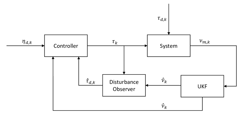
Fig. 2: Observer framework

For traceability, in the following, pseudocode is presented. The code should give clear instructions to reconstruct the entire framework. Initialization parameters are depicted in Table 1. Tuning parameters such as $\Gamma_{1}$, $\Gamma_{2}$, $\Gamma_{3}$, $\alpha$, $\beta$, and $\kappa$, used for this study, are just a recommendation. However, the adaptive gains should be adjusted if the sensor measurements have a lower sampling frequency. This will be discussed in more detail in section 3.2.

Algorithm 1 Pseudocode

1:while $\mathrm{observation}=\mathrm{True}$ do

2:     $\bm{\hat{\tau}_{d,k}}=\bm{\zeta}_{k}+\bm{T}\bm{\hat{\nu}}_{k}$

3:     $\bm{\zeta}_{k+1}=\bm{\zeta}_{k}+\Delta t\left(-\bm{T}\bm{\nu}_{k+1}(\bm{\tau_{d,k}}=\bm{\zeta}_{k}+\bm{T}\bm{\hat{\nu}}_{k})\right)$

4:     $\bm{\mathcal{X}}_{0,k}=\bm{\mathrm{\hat{\nu}}}_{k}$

5:     $\bm{\mathcal{X}}_{i,k}=\bm{\hat{\nu}}_{k}+\left(\sqrt{(L+\lambda)}\bm{P}_{k}\right)_{i},\ i=1,...,L$

6:     $\bm{\mathcal{X}}_{i,k}=\bm{\hat{\nu}}_{k}-\left(\sqrt{(L+\lambda)}\bm{P}_{k}\right)_{i-L},\ i=L+1,...,2L$

7:     $\bm{\check{\nu}}_{k}=\sum_{i=0}^{2L}W^{m}_{i}\bm{\nu}_{k+1}(\bm{\mathcal{X}}_{i,k})$

8:     $\bm{\check{\nu}}_{m,k}=\sum_{i=0}^{2L}W^{m}_{i}\bm{\nu}_{m,k}(\bm{\mathcal{X}}_{i,k})$

9:     $\bm{P}_{x,k}=\sum_{i=0}^{2L}W^{c}_{i}\left(\bm{\nu}_{k+1}(\bm{\mathcal{X}}_{i,k})-\bm{\check{\nu}}_{k}\right)\left(\bm{\nu}_{k+1}(\bm{\mathcal{X}}_{i,k})-\bm{\check{\nu}}_{k}\right)^{\top}$

10:     $\bm{P}_{y,k}=\sum_{i=0}^{2L}W^{c}_{i}\left(\bm{\nu}_{m,k}(\bm{\mathcal{X}}_{i,k})-\bm{\check{\nu}}_{m,k}\right)\left(\bm{\nu}_{m,k}(\bm{\mathcal{X}}_{i,k})-\bm{\check{\nu}}_{m,k}\right)^{\top}$

11:     $\bm{P}_{xy,k}=\sum_{i=0}^{2L}W^{c}_{i}\left(\bm{\nu}_{k+1}(\bm{\mathcal{X}}_{i,k})-\bm{\check{\nu}}_{k}\right)\left(\bm{\nu}_{m,k}(\bm{\mathcal{X}}_{i,k})-\bm{\check{\nu}}_{m,k}\right)^{\top}$

12:     $\bm{K}_{k}=\bm{P}_{xy,k}\bm{P}_{y,k}^{-1}$

13:     $\bm{\hat{\nu}}_{k+1}=\bm{\check{\nu}}_{k}+\bm{K}_{k}(\nu_{m,k}-\bm{\check{\nu}}_{m,k})$

14:     $\bm{P}_{k+1}=\bm{P}_{x,k}-\bm{K}_{k}\bm{P}_{y,k}\bm{P}_{x,k}$

15:end while

3 Method and setup

This study is conducted with the specifications of the milliAmpere ferry. MilliAmpere is Norway’s first driverless ferry and part of the Autoferry project of the Norwegian University of Science and Technology [14].

3.1 Ferry specification

The hydrodynamic parameters and the entries of the mass matrix are identified in [15] by using datasets consisting of velocity measurements $\bm{\nu}_{m}$ of the ship, rotational velocity measurements of the propellers, and azimuth angle measurements of the thrusters. For this purpose, techniques such as optimal control, regularization, and cross-validation are used. The identified parameters are shown in Table 2.

3.2 Scenario description

The observer framework was tested in several scenarios corresponding to different severity levels of the environmental disturbances. However, in the current work, only the most severe scenario with model and measurement uncertainties is discussed to showcase the capability of the framework. For this purpose, the control input $\tau$ is set to zero in order to visualize the environmental impact.

Table 3 provides an overview of the parametrization of the scenario, including parameters such as environmental forces and their impact angles, the covariance matrix $\bm{Q}$ of model uncertainties, the covariance matrix $\bm{R}$ of measurement uncertainties, the covariance matrix $\bm{H}$ to simulate the disturbances as a stochastic process, the observation gains $\Gamma_{i}$ for $i=1,2,3$, and the time step $\Delta t$ between each measurement. Note that $\bm{I}_{3\times 3}$ expresses the identity matrix.

Since the environmental forces depend on the impact surface, real data regarding wind, waves, and sea currents differs from ship to ship and is thus difficult to find. Hence, rough calculations of possible environmental forces $\bar{F}_{\mathrm{wind}}$, $\bar{F}_{\mathrm{wave}}$, and $\bar{F}_{\mathrm{current}}$ were made by the theory of [12] under consideration of storm values. Furthermore, sea current velocity values for severe situations are adopted from [16].

Other simulations have shown that the adaptive gains $\Gamma_{i}$ should be adjusted to the measurement timestep $\Delta t$. A higher sampling frequency, i.e., a lower timestep, offers the possibility to increase the adaptive gains very high. However, reducing the sampling frequency results in a reciprocal effect. If the adaptive gains are improperly adjusted to the sampling frequency, the observer turns unstable. Despite that, a timestep of $\Delta t=0.1\,\mathrm{s}$ still enables $\Gamma_{i}=18$, which is absolutely sufficient for a fast adaptation.

The simulated environmental influences are defined as

$$\bm{\tau}_{\mathrm{wind}}=\begin{bmatrix}\bar{F}_{\mathrm{wind}}\cos(\gamma_{\mathrm{wind}}-\psi)\left(1+\frac{1}{10}\sin(5t)\right)\\[3.0pt] -\bar{F}_{\mathrm{wind}}\sin(\gamma_{\mathrm{wind}}-\psi)\left(1+\frac{1}{10}\sin(5t)\right)\\[3.0pt] \bar{F}_{\mathrm{wind}}\sin(2(\gamma_{\mathrm{wind}}-\psi))\left(1+\frac{1}{10}\sin(5t)\right)\frac{L}{4}\end{bmatrix},$$ (66a)

$$\bm{\tau}_{\mathrm{wave}}=\begin{bmatrix}\bar{F}_{\mathrm{wave}}\cos(\gamma_{\mathrm{wave}}-\psi)\left(1+\sin(t)\right)\\[3.0pt] -\bar{F}_{\mathrm{wave}}\sin(\gamma_{\mathrm{wave}}-\psi)\left(1+\sin(t)\right)\\[3.0pt] 0\end{bmatrix},$$ (66b)

$$\bm{\tau}_{\mathrm{current}}=\begin{bmatrix}\bar{F}_{\mathrm{current}}\cos(\gamma_{\mathrm{current}}-\psi)\left(1-e^{-\frac{t}{T_{s}}})\right)\\[3.0pt] -\bar{F}_{\mathrm{current}}\sin(\gamma_{\mathrm{current}}-\psi)\left(1-e^{-\frac{t}{T_{s}}})\right)\\[3.0pt] 0\end{bmatrix}.$$ (66c)

Note that the impact angles $\gamma_{i}$ of wind, waves, and currents are related to the $x$-axis of the global coordinate system. Since the waves are affected by wind, they have approximately the same direction. Furthermore, it is expected that the torque induced by the environment is mainly influenced by the wind. Hence, it is assumed that the wind force in the sway direction describes the torque dependent on $\cos(\gamma_{\mathrm{wind}}-\psi)$ impacting half of the ship’s length. Note that the identity $\cos(\gamma_{\mathrm{wind}}-\psi)\sin(\gamma_{\mathrm{wind}}-\psi)=\frac{1}{2}\sin(2(\gamma_{\mathrm{wind}}-\psi))$ is valid. In addition, an oscillating force is superposed to the wind’s mean force in order to simulate a pulsating wind behavior. The waves are simulated as oscillating forces, where smaller waves are superposed with larger waves. It is assumed that the sea currents do not exhibit highly dynamic behavior. Therefore, they are simulated as an exponentially decaying force.

4 Results and discussions

To evaluate the sensitivity of the predicted trajectory concerning $\bm{Q}$, we conducted two simulations, one without any model uncertainty (given by (3)) and another with uncertainty containing covariance $\bm{Q}$. Fig. 3 compares the resulting trajectories. The corresponding surge, sway, and rotational speeds are depicted in Fig. 4. It can be clearly seen that an erroneous model can lead to a completely different trajectory, a problem that the observer framework has to deal with. In Fig. 5, the measured states, the real system states considering model uncertainty with covariance $\bm{Q}$, and the filtered measurements from the UKF are visualized. It is obvious that the measurements are significantly noisy, and the UKF successfully smoothens them. Furthermore, a closer look at Fig. 4 and Fig. 5 reveals that the filtered measurements from the UKF show similar behavior to the system states of the model dynamics without uncertainty. Using the filtered measurements of the UKF and propagating them through the proposed disturbance observer leads to accurate estimations of the real disturbances, as shown in Fig. 6. Since the estimations are very close to the real values, a zoomed fraction is additionally depicted. Fig. 7 shows the results of the observer framework where the disturbances are simulated with superposed Gaussian noise containing covariance $\bm{H}$. The estimations of the observer represent a smoothed version of the noisy environmental disturbances. This characteristic could be beneficial for control concepts since actuators should not frequently peak to their limits. The relative error of Fig. 6 concerning the maximum absolute value is showcased in Fig. 8 and is represented by

$$z_{r,i}=\frac{\tau_{d,i}-\hat{\tau}_{d,i}}{\max(|\tau_{d,i}|)},\ \ \ \ \ i=1,2,3.$$ (67)

The relation to the maximum absolute value is chosen since the relative error leads to high peaks if the zero value is crossed. Furthermore, Fig. 8 contains the comparison of simulations with various model uncertainties $\bm{Q}_{1}=10^{3}\bm{I}$, $\bm{Q}_{2}=10^{4}\bm{I}$, $\bm{Q}_{3}=3\cdot 10^{4}\bm{I}$, and $\bm{Q}_{4}=10^{5}\bm{I}$. Fig. 9 visualize the equal adaptation speed by adjusting $\Gamma_{i}$ identically due to the formulation of the error dynamics of the observer. For this purpose, the disturbances $\bm{\tau_{d}}$ are simulated with equal behavior as an exponentially decaying process. Hence, the representation depicted in Fig. 9 is independent of the chosen simulation scenario. It can be seen that a synchronization of the observed disturbances is guaranteed. This property might be beneficial since controllers can be supplied with consistent estimations.

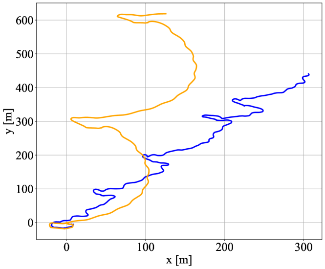
Fig. 3: Trajectories with ( ), and without ( ) model uncertainty for the time interval $t_{\mathrm{end}}-t_{0}=200\,\mathrm{s}$. This figure shows how unreliable the considered model dynamics are.

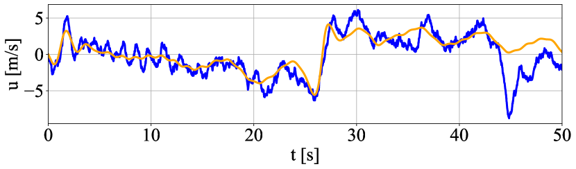
(a) surge

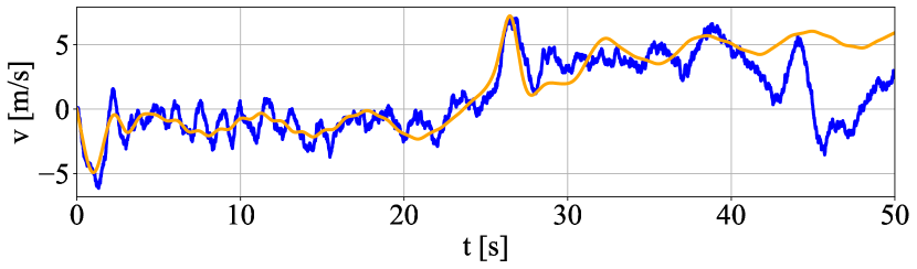
(b) sway

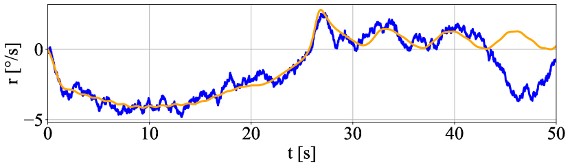
(c) rotational speed

Fig. 4: States with $\bm{Q}$ ( ), and without model uncertainty ( ).

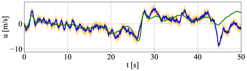
(a) surge

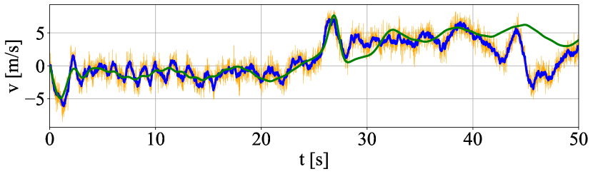
(b) sway

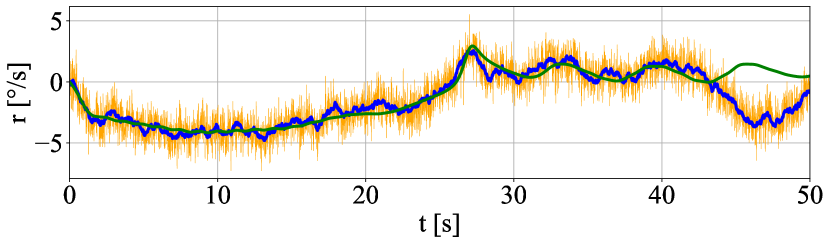
(c) rotational speed

Fig. 5: Measured states with measurement noise ( ), real states ( ), and the filtered states from the UKF ( ).

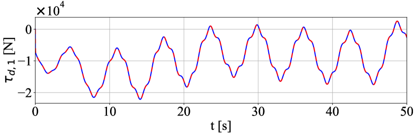
(a) observed disturbances concerning surge

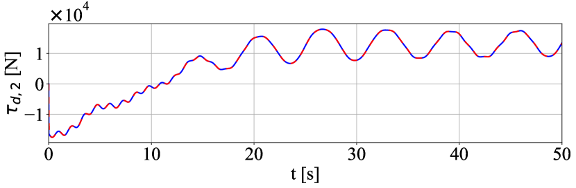
(b) observed disturbances concerning sway

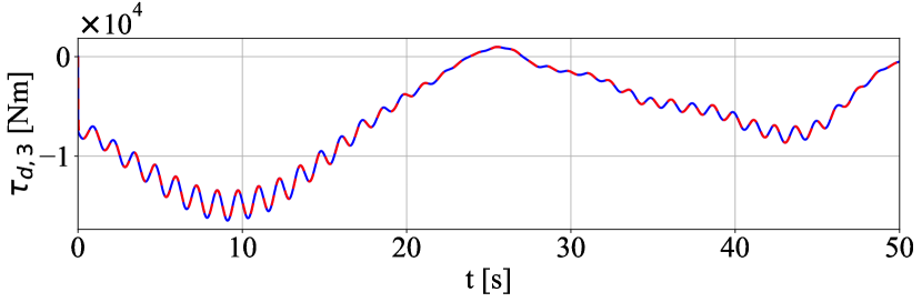
(c) observed disturbances concerning rotational speed

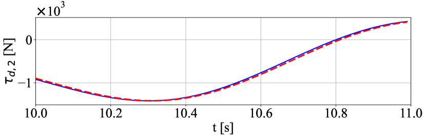
(d) fraction of the observed disturbance $\tau_{d,2}$

Fig. 6: Observed disturbances $\bm{\hat{\tau}_{d}}$ ( ) compared to the real disturbances $\bm{\tau_{d}}$ ( ).

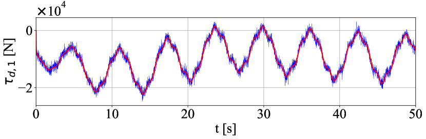
(a) observed disturbances concerning $u$

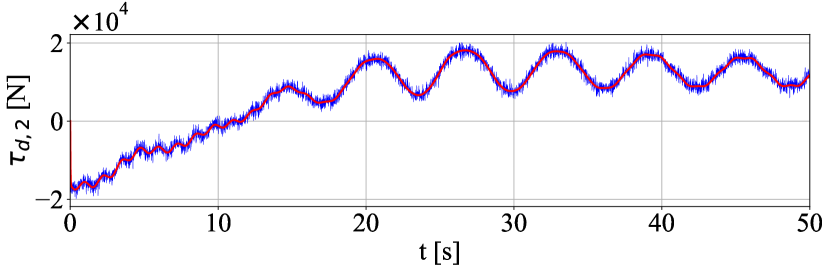
(b) observed disturbances concerning $v$

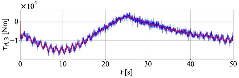
(c) observed disturbances concerning $r$

Fig. 7: Observed disturbances $\bm{\hat{\tau}_{d}}$ ( ) compared to the real disturbances $\bm{\tau_{d}}$ ( ). Here, the real disturbances are additionally simulated with superposed Gaussian noise containing covariance $\bm{H}$.

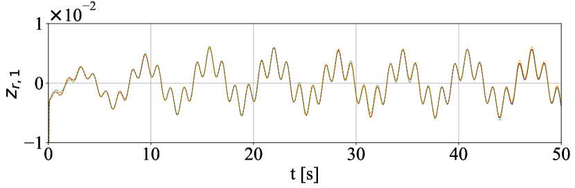
(a) relative error concerning surge

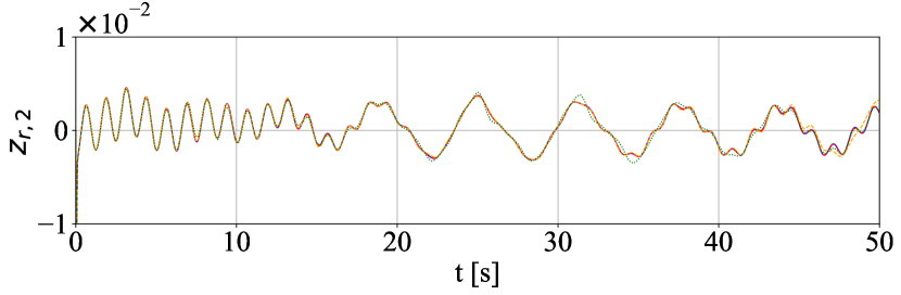
(b) relative error concerning sway

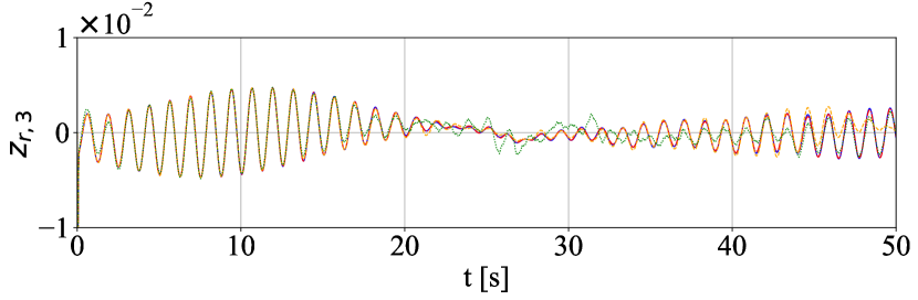
(c) relative error concerning rotational speed

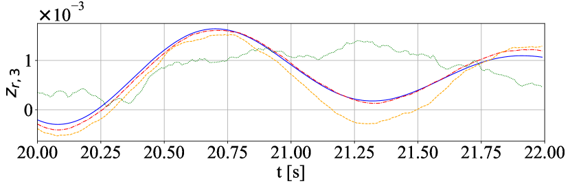
(d) fraction of the relative error $z_{r,3}$

Fig. 8: Relative Error of the observer framework for different model uncertainties with respect to the maximum absolute value. The uncertainties are scaled as $\bm{Q}_{1}$ ( ), $\bm{Q}_{2}$ ( ), $\bm{Q}_{3}$ ( ), and $\bm{Q}_{4}$ ( ).

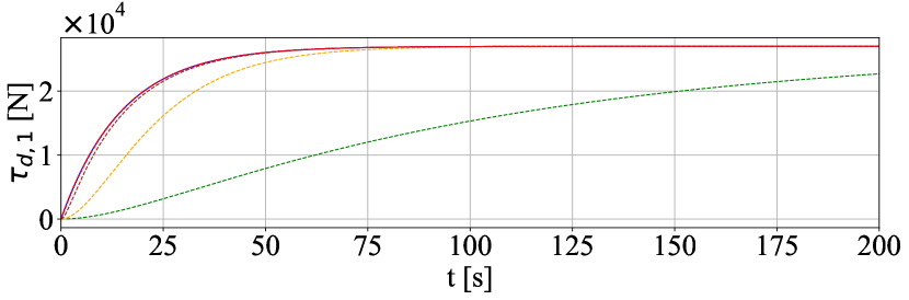
(a) observed disturbances concerning surge

(b) observed disturbances concerning sway

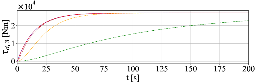
(c) observed disturbances concerning rotational speed

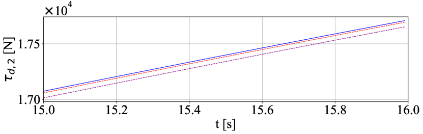
(d) fraction of the observed disturbance $\tau_{d,2}$

Fig. 9: Comparison of different $\Gamma_{i}$, for $i=1,2,3$ with $\Gamma_{i}=0.01$ ( ), $\Gamma_{i}=0.1$ ( ), $\Gamma_{i}=1$ ( ), $\Gamma_{i}=10$ ( ), $\Gamma_{i}=30$ ( ), and the real disturbances ( ). This simulation is designed such that all disturbances represent equal behavior for the purpose of better comparability. Here, it is shown that the designed observer allows a convenient adjustment of the adaptive gains.

5 Conclusion

The proposed disturbance observer framework proved its capability for precisely reconstructing the environmental impact of wind, waves, and sea currents despite an unreliable model and highly noisy measurements. The main takeaway from the current work can be itemized as follows:

• Under consideration of a discrete, temporal sequence of measurements, the framework can accurately observe the real disturbances despite very low sampling rates.

• The Unscented Kalman Filter (UKF) smoothens the noisy measurements. Subsequently, the smoothed measurements are propagated through the disturbance observer. As a result, the observed disturbances have no noisy characteristics. This property might be beneficial for controllers since triggering actuators frequently to their limits has a corrosive character.

• Since the UKF also smoothes model uncertainties, the observer framework correctly reconstructs the disturbances despite using an erroneous model.

• The formulation of the observer’s error dynamics allows the user a convenient approach for synchronizing the adaptation speed concerning the observed disturbances.

Appendix

Table 1: Initialization

Parameter	Value
$\bm{\hat{\nu}}_{0}$	$E[\bm{\nu}_{0}]$
$P_{\mathrm{init}}$	$0.1$
$\bm{P}_{0}$	$P_{\mathrm{init}}\cdot\mathrm{eye}(L,L)$
$\Gamma_{1}$	$50$
$\Gamma_{2}$	$50$
$\Gamma_{3}$	$50$
$\bm{\zeta}_{0}$	$\mathrm{zeros}(L,1)$
$\alpha$	$10^{-3}$
$\beta$	$2$
$\kappa$	$0$

Table 2: Values and units of the parameters of the milliAmpere ferry

Par	Value	Unit	Par	Value	Unit
$m_{11}$	2389.657	kg	$m_{22}$	2533.911	kg
$m_{23}$	62.386	kg	$m_{32}$	28.141	kg
$m_{33}$	5068.910	$\mathrm{kg\cdot m^{2}}$	$X_{u}$	-27.632	$\frac{kg}{s}$
$X_{|u|u}$	-110.064	$\frac{kg}{s}$	$X_{uuu}$	-13.965	$\frac{kg}{s}$
$Y_{v}$	-52.947	$\frac{kg}{s}$	$Y_{|v|v}$	-116.486	$\frac{kg}{s}$
$Y_{vvv}$	-24.313	$\frac{kg}{s}$	$Y_{|r|v}$	-1540.383	$\frac{kg}{s}$
$Y_{r}$	24.732	$\frac{kg}{s}$	$Y_{|v|r}$	572.141	$\frac{kg}{s}$
$Y_{|r|r}$	-115.457	$\frac{kg}{s}$	$N_{v}$	3.5241	$\frac{kg}{s}$
$N_{|v|v}$	-0.832	$\frac{kg}{s}$	$N_{|r|v}$	336.827	$\frac{kg}{s}$
$N_{r}$	-122.860	$\frac{kg}{s}$	$N_{|r|r}$	-874.428	$\frac{kg}{s}$
$N_{rrr}$	0.000	$\frac{kg}{s}$	$N_{|v|r}$	-121.957	$\frac{kg}{s}$

Table 3: Value and units of the Simulation parameters

Par	Value	Unit	Description
$\bm{Q}$	30000$\cdot\bm{I}_{3\times 3}$	-	Covariance matrix
$\bm{R}$	$\bm{I}_{3\times 3}$	-	Covariance matrix
$\bm{H}$	1000$\cdot\bm{I}_{3\times 3}$	-	Covariance matrix
$\Gamma_{1}$	50	-	Adaptive gain
$\Gamma_{2}$	50	-	Adaptive gain
$\Gamma_{3}$	50	-	Adaptive gain
$\Delta t$	0.01	s	Timestep
$\bar{F}_{\mathrm{wind}}$	10000	N	Wind force
$\bar{F}_{\mathrm{wave}}$	8000	N	Wave force
$\bar{F}_{\mathrm{current}}$	18000	N	Current force
$\gamma_{\mathrm{wind}}$	135	deg	Wind angle
$\gamma_{\mathrm{wave}}$	155	deg	Wave angle
$\gamma_{\mathrm{current}}$	300	deg	Current angle
$L$	5	m	Ship length
$T_{s}$	15	s	Time constant
$\bm{\eta}$	$[0,0,30]^{\top}$	[m,m,deg]	Initial position
			and heading
$\bm{\nu}$	$[0,0,0]^{\top}$	[$\frac{\mathrm{m}}{\mathrm{s}}$,$\frac{\mathrm{m}}{\mathrm{s}}$,$\frac{\mathrm{deg}}{\mathrm{s}}$]	Initial velocity

References

- [1] K. Do, Z. Jiang, J. Pan, Global partial-state feedback and output-feedback tracking controllers for underactuated ships, Systems & Control Letters 54 (10) (2005) 1015–1036. doi:10.1016/j.sysconle.2005.02.014.
- [2] X. Wei, L. You, H. Zhang, X. Hu, J. Han, Disturbance observer based control for dynamically positioned ships with ocean environmental disturbances and actuator saturation, International Journal of Robust and Nonlinear Control 32 (7) (2022) 4113–4128. doi:10.1002/rnc.6023.
- [3] J. Huang, C. Wen, W. Wang, Y.-D. Song, Global stable tracking control of underactuated ships with input saturation, Systems & Control Letters 85 (2015) 1–7. doi:10.1016/j.sysconle.2015.07.002.
- [4] Y. Bouteraa, K. A. Alattas, S. Mobayen, M. Golestani, A. Ibrahim, U. Tariq, Disturbance Observer-Based Tracking Controller for Uncertain Marine Surface Vessel, Actuators 11 (5) (2022) 128. doi:10.3390/act11050128.
- [5] N. T. Duong, N. Q. Duy, Adaptive backstepping control for ship nonlinear active fin system based on disturbance observer and neural network, International Journal of Electrical and Computer Engineering (IJECE) 12 (2) (2022) 1392. doi:10.11591/ijece.v12i2.pp1392-1401.
- [6] D. Xu, Z. Liu, X. Zhou, L. Yang, L. Huang, Trajectory Tracking of Underactuated Unmanned Surface Vessels: Non-Singular Terminal Sliding Control with Nonlinear Disturbance Observer, Applied Sciences 12 (6) (2022) 3004. doi:10.3390/app12063004.
- [7] K. D. Do, Practical control of underactuated ships, Ocean Engineering 37 (13) (2010) 1111–1119. doi:10.1016/j.oceaneng.2010.04.007.
- [8] N. Gu, D. Wang, Z. Peng, J. Wang, Q.-L. Han, Disturbance observers and extended state observers for marine vehicles: A survey, Control Engineering Practice 123 (2022) 105158. doi:10.1016/j.conengprac.2022.105158.
- [9] C. Huang, X. Zhang, Y. Deng, G. Zhang, Robust Dynamic Positioning Control of Marine Ships via a Disturbance Observer, Proceedings of the Twenty-ninth (2019) International Ocean and Polar Engineering Conference (2019).
- [10] Z. Peng, D. Wang, J. Wang, Data-Driven Adaptive Disturbance Observers for Model-Free Trajectory Tracking Control of Maritime Autonomous Surface Ships, IEEE Transactions on Neural Networks and Learning Systems 32 (12) (2021) 5584–5594. doi:10.1109/tnnls.2021.3093330.
- [11] U. B. Trivedi, M. Bhatt, P. Srivastava, Prevent Overfitting Problem in Machine Learning: A Case Focus on Linear Regression and Logistics Regression, in: Innovations in Information and Communication Technologies (IICT-2020), Springer International Publishing, 2021, pp. 345–349. doi:10.1007/978-3-030-66218-9\_40.
- [12] T. I. Fossen, Handbook of Marine Craft Hydrodynamics and Motion Control, John Wiley & Sons, Ltd, 2011. doi:10.1002/9781119994138.
- [13] S. J. Julier, J. K. Uhlmann, New extension of the Kalman filter to nonlinear systems, in: I. Kadar (Ed.), SPIE Proceedings, SPIE, 1997. doi:10.1117/12.280797.
- [14] E. F. Brekke, E. Eide, B.-O. H. Eriksen, E. F. Wilthil, M. Breivik, E. Skjellaug, Øystein K. Helgesen, A. M. Lekkas, A. B. Martinsen, E. H. Thyri, milliAmpere: An Autonomous Ferry Prototype, Journal of Physics: Conference Series (2022).
- [15] A. A. Pedersen, Optimization Based System Identification for the milliAmpereFerry, Master’s thesis, Norwegian University of Science and Technology (2019).
- [16] Y. Wang, W. Du, G. Li, Z. Li, J. Hou, H. Hu, Efficient Ship Maneuvering Prediction with Wind, Wave and Current Effects, in: Advances in Transdisciplinary Engineering, IOS Press, 2022. doi:10.3233/atde220115.