MEAL: Stable and Active Learning for Few-Shot Prompting

Abstract

Few-shot classification has made great strides due to foundation models that, through priming and prompting, are highly effective few-shot learners. However, this approach has high variance both across different sets of few shots (data selection) and across different finetuning runs (run variability). This is problematic not only because it impedes the fair comparison of different approaches, but especially because it makes few-shot learning too unreliable for many real-world applications. To alleviate these issues, we make two contributions for more stable and effective few-shot learning: First, we propose novel ensembling methods and show that they substantially reduce run variability. Second, we introduce a new active learning (AL) criterion for data selection and present the first AL-based approach specifically tailored towards prompt-based learning. In our experiments, we show that our combined method, MEAL (Multiprompt finetuning and prediction Ensembling with Active Learning), improves overall performance of prompt-based finetuning by 2.3 points on five diverse tasks. We publicly share our code and data splits in https://github.com/akoksal/MEAL.

MEAL: Stable and Active Learning for Few-Shot Prompting

1 Introduction

Pretrained language models (PLMs) are effective few-shot learners when conditioned with a few examples in the input (Brown et al., 2020; Min et al., 2022, i.a.) or finetuned with a masked language modeling objective on samples converted into cloze-style phrases Schick and Schütze (2021a); Gao et al. (2021). Prompt-based finetuning is especially promising as it enables researchers to train relatively small models as few-shot classifiers that can make accurate predictions with a minimal investment of time and effort.

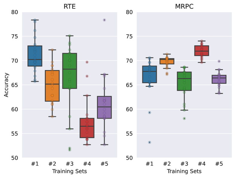
Figure 1: Multiprompt results with 32 examples for ALBERT on RTE and MRPC. Prompt-based finetuning has large variance depending on training data selection and random initialization. The accuracy difference can be up to 23.5 with different random seeds (RTE #3) and 13.7 with different training sets (RTE #1 vs #4).

However, prompt-based finetuning suffers from high variance. We observe two causes in our experiments: run variability (different seeds) and data selection (different training sets). Figure 1 illustrates this for five equal-size training sets and 20 runs for RTE Dagan et al. (2006) and MRPC Dolan and Brockett (2005). Both sources of variance are of particular concern in few-shot learning. We may get lucky and select a “good” training set. But because no dev set is available there is also a high risk of selecting a “bad” training set, resulting in much lower performance than possible for the available annotation budget. In addition, run variability is a great methodological problem because it means that the exact same experimental setup (except for different random seeds, causing variance in the order of training examples and dropout layers) will give different results. This makes fair comparison of different algorithms and architectures difficult.

We propose new approaches to few-shot learning that address both sources of variance. We first focus on run variability and show based on loss/accuracy surface visualizations Li et al. (2018) that run variability in few-shot learning is different from fully-supervised settings: solutions proposed for finetuning PLMs Mosbach et al. (2021) do not work for few-shot prompt-based finetuning. Thus, we propose ensemble techniques to stabilize finetuning for different runs. After mitigating the effects of run variability via a more stable finetuning mechanism, we are able to address training data selection. We modify existing active learning (AL) algorithms and propose a novel approach for selecting training examples that outperforms prior algorithms – not just in terms of final accuracy, but also regarding the diversity and representativeness of selected examples. In general, we are, to the best of our knowledge, the first to develop AL algorithms tailored to prompt-based finetuning.

We combine our contributions – decrease run variance and better training sets for improved performance and stability of few-shot classification – in MEAL (Multiprompt finetuning and prediction Ensembling with Active Learning). MEAL improves performance of prompt-based finetuning by 2.3 points on five tasks. Contributions:

1. We propose a training procedure that produces a single few-shot classification model with multiple prompts on top of PET Schick and Schütze (2021a). This reduces model space complexity and improves overall performance.

2. We show that run variability is a big problem in few-shot classification and conduct an exhaustive analysis of why existing solutions do not apply to few-shot prompt-based finetuning. We propose ensemble techniques to improve run stability.

3. We propose a novel AL method for data selection that outperforms prior AL work and random selection. Our work is the first to demonstrate that AL is beneficial in prompt-based learning.

2 Related Work

Few-shot classification with language model prompting. GPT-3 Brown et al. (2020) prepends examples as conditioning to the input during inference, without parameter updates. PET Schick and Schütze (2021a, b) follows a similar approach with finetuning and achieves comparable results, with fewer parameters. LM-BFF Gao et al. (2021) and ADAPET Tam et al. (2021) extend PET.

Instability. There are two sources of instability in finetuning PLMs for few-shot classification: run variability and data selection. Run variability comes from finetuning PLMs with random seeds. Mosbach et al. (2021) and Dodge et al. (2020a) show that finetuning PLMs is an unstable process for fully supervised training. Recently, Zheng et al. (2022) demonstrated that few-shot finetuning also exhibits run variability but their experiments have different training sets in a cross-validation scenario. They do not address how much instability comes from finetuning vs. data selection. Our findings suggest that the instability issue exists in few-shot training for the same training set, and existing solutions for fully supervised settings (e.g., Dodge et al. (2020a), Mosbach et al. (2021)) do not stabilize finetuning for few-shot classification. We propose the run ensemble method to improve the stability of few-shot classification. The second type of instability is training data selection; we target this issue with AL.

Active Learning. As collecting labeled data is time-consuming and costly, AL has been a crucial part of supervised learning Cohn et al. (1996); Settles (2009); Rotman and Reichart (2022). Apart from efficiency in data labeling, we show that some training sets have significantly worse performance than others for few-shot classification. Zhao et al. (2021a) also show that the selection of the few shots matters a lot. Hence, we follow an AL setup to select informative and diverse training sets for few-shot classification. Schröder et al. (2022) recently showed that uncertainty AL achieves significant improvements for fully supervised settings in PLMs. Following this, we modify a variety of AL algorithms including prior works such as CAL Margatina et al. (2021) and BADGE Ash et al. (2020) for few-shot prompt-based finetuning, and propose a novel AL algorithm, IPUSD.

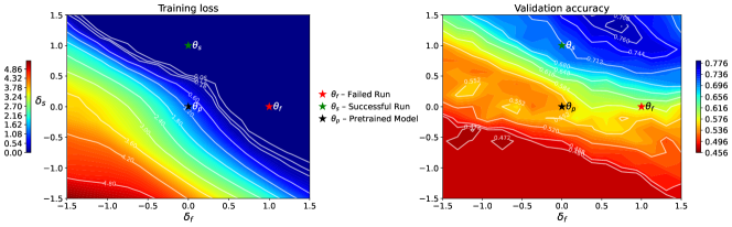
Figure 2: Loss and validation accuracy surface visualizations for two RTE runs with the same training set. Left (training loss): The two models $\theta_{s}$ and $\theta_{f}$ have similar loss – they are both located in the upper right blue zero-loss triangle. Right (validation accuracy): The successful model $\theta_{s}$ performs much better than the failed model $\theta_{f}$.

3 Multiprompt Finetuning

Let $M$ be a masked PLM, $T$ its vocabulary, and $\textit{MASK}\in T$ the mask token. We use Pattern-Exploiting Training (PET) Schick and Schütze (2021a) for prompt-based finetuning experiments on few-shot classification without knowledge distillation and unlabeled data. Patterns ($\mathcal{P}$) transform an input $x$ into a cloze-style phrase $x_{p}$ with a single mask. Verbalizers ($V$) convert each label $l\in L$ into a single token $s_{l}\in T$, representing the task-specific meaning of the output label.

Our prediction for a label is its probability, according to the PLM, as a substitution for the mask:
ab$P(y|x)=\frac{\exp s_{m}(V(y)|x_{p})}{\sum_{y^{*}\in L}\exp s_{m}(V(y^{*})|x_{p})}$
where $s_{m}$ gives the raw score of $V(y)$ from a PLM $M$ for the MASK position in the cloze-style phrase of the input. Using the cross-entropy loss of $P$, PET trains a separate model for each prompt (i.e., single prompt finetuning). In inference, it ensembles model predictions by logit averaging.

We propose multiprompt finetuning, a modified PET that trains a single model $M$ on all prompts for a task simultaneously. During inference time, we also use ensembling with logit averaging across prompts. However, our approach generates a single finetuned model regardless of the number of prompts. Compared to PET, this reduces runtime, memory, and overall complexity.

4 Run Variability

In few-shot classification, finetuning PLMs such as ALBERT Lan et al. (2020) with an MLM objective on samples converted into cloze-style phrases Schick and Schütze (2021b) performs comparably to much larger GPT-3 Brown et al. (2020). Just as prompting methods are sensitive to data order Lu et al. (2022) and label distributions Zhao et al. (2021b), finetuning PLMs also exhibits sensitivity and instability as shown by Dodge et al. (2020b) for a fully supervised setting.

We show that the instability of finetuning PLMs also exists in few-shot prompt-based finetuning. Even though prompt-based finetuning does not introduce new parameters like classifier heads as in fully supervised classification, there is variance from dropout and training data order. We conduct experiments with multiprompt finetuning with default PET Schick and Schütze (2021a) settings without knowledge distillation. Figure 1 shows that runs with different random seeds for the same training set can vary by as much as 23.5 points.

Mosbach et al. (2021) suggest that longer training with a low learning rate and warm-up reduces run variability of PLMs. Their main motivation is to avoid models ending up in suboptimal training loss regions. However, this is not valid in few-shot prompt tuning as the number of training examples is low, and finetuning achieves almost zero training loss quickly. Our initial experiments show that longer training does reduce the standard deviation between different runs, but that it also causes lower mean accuracy for most tasks, of up to 7.3 points.

In Figure 2, we analyze run variability, by creating a training loss and validation accuracy surface visualization of two RTE runs with the same training set and multiprompt finetuning. The failed model $\theta_{f}$ (red) achieves 58.5% validation accuracy while the successful model $\theta_{s}$ (green) achieves 71.5%. The two models only differ in finetuning random seed. The figure illustrates the training loss and validation accuracy surfaces for combinations of the model weights of the pretrained model ($\theta_{p}$), the failed model ($\theta_{f}$), and the successful model ($\theta_{s}$). We create a two-dimensional space based on $f(a,b)=F(\theta_{p}+a\delta_{f}+b\delta_{s})$, where $\delta_{f}=\theta_{f}-\theta_{p}$, $\delta_{s}=\theta_{s}-\theta_{p}$, and $F$ is loss (left) or accuracy (right). We use 16 values for $a$ and $b$ to plot loss and accuracy surface forms.

Figure 2 shows that there is a large region with $\leq$1e-4 training loss (left graph, dark blue) that includes $\theta_{f}$ and $\theta_{s}$. However, most of this region is suboptimal in terms of validation accuracy (right graph). This indicates that our instability problem differs from fully supervised finetuning where large learning rates often result in suboptimal training loss; in contrast, we observe $\approx$0 training loss for each run, including failed ones. Therefore, longer training with a low learning rate and warm-up only leads to finetuned models ending up in a similar region with lower variance, but it causes suboptimal validation accuracy scores; see §6 for more details.

To overcome run variability, we propose two ensemble models: We ensemble the logits over runs in ENSEMBLE_pred and take the average of parameters over runs in ENSEMBLE_para. We will show that, for five tasks, these (i) reduce the effect of failed runs and run variability and (ii) achieve higher accuracy than accuracy averaged over runs.

The prediction of ENSEMBLE_pred for $x$ is:
ab$P(y|x)=\mbox{s}(\sum\limits_{r=1}^{R}[\sum\limits_{p\in\mathcal{P}}F_{r}(y|x_{p})]/(R*|\mathcal{P}|))$
where s is softmax, R is the number of runs, $\mathcal{P}$ is the set of prompts, and $F_{r}$ gives, for the finetuned model in run $r$, the logit of each class for the input $x$ with prompt $p$.

Following work on averaging deep networks Izmailov et al. (2018), we average each parameter of the finetuned PLMs across runs, resulting in a single model. The prediction of ENSEMBLE_para for $x$ is the prediction of this single model.

5 Data Selection

Another important source of variance for few-shot classification is training data selection. Figure 1 shows this effect: validation accuracy greatly varies, with a difference of up to 13.7.

Figure 3 shows how we modify AL algorithms for data selection in few-shot prompt-based finetuning. First, we use a PLM to get contextual embeddings, logits, and probabilities for each unlabeled example in a zero-shot setting. We exploit here that, due to the cloze-style format, PLMs can make predictions before any finetuning. Second, we apply modified AL algorithms for prompts. We select all examples at once to simplify the selection process. For each task, we select $16*L$ training examples, where $L$ is the number of labels.

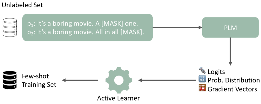
Figure 3: Our modified active learning pipeline for data selection is illustrated with an example sentence and two prompts for sentiment analysis. The PLM outputs several features in a zero-shot manner. AL selects a few-shot training set based on these output features.

5.1 Prior-Work Active Learning

We use a range of prior-work AL algorithms, including random, uncertainty-only (e.g., entropy) and combined approaches (e.g., BADGE). Although these are prior-work, adapting them to a prompt-based setup is non-trivial; e.g., for BADGE it requires concatenating gradient vectors across prompts. Therefore, this adaptation is one of the contributions of our paper. Importantly, none of the prior-work leverages the prediction variety across different prompts.

Random selection draws random examples from an unlabeled set. We report random selection results with five different seeds.

Entropy Roy and McCallum (2001) computes the entropy score of an example by summing the entropy across prompts. We then select examples with highest entropy scores.
a$\mbox{e}(x_{i})\!=\!\sum\limits_{j=1}^{j=L}\sum\limits_{p\in\mathcal{P}}\!-\!P(y\!=\!l_{j}|x_{i,p})\ln P(y\!=\!l_{j}|x_{i,p})$
where $L$ is the number of labels, $\mathcal{P}$ is the set of prompts, and $x_{i,p}$ is input $x_{i}$ with pattern $p$.

Breaking Ties (BT) Luo et al. (2004) selects examples with minimum difference between the highest two probability classes.
ab$\mbox{bt}(x_{i})=\sum\limits_{p\in\mathcal{P}}P(y=l_{1}|x_{i,p})-P(y=l_{2}|x_{i,p})$
where $l_{1}$ and $l_{2}$ are the labels with highest and second highest probability for $x_{i,p}$.

Lowest Confidence (LC) Culotta and McCallum (2005) calculates lc as the sum of probability scores for the predicted class across prompts. We select examples with lowest lc. lc and bt give the same order when there are two labels.
ab$\mbox{lc}(x_{i})=\sum\limits_{p\in\mathcal{P}}\max\{P(y=l_{j}|x_{i,p}):j=1..L\}$

Contrastive AL (CAL) Margatina et al. (2021) selects examples with the highest KL divergence between the example and its $M$ nearest neighbors in the PLM contextual embedding space.
ab$\mbox{cal}(x_{i})=\sum\limits_{m=1}^{m=M}\sum\limits_{p\in\mathcal{P}}\mbox{KL}(P(y|x_{m,p})||P(y|x_{i,p}))$

Batch AL by Diverse Gradient Embeddings (BADGE) Ash et al. (2020) uses as representation the gradient of the cross entropy loss, conditioned on the one-hot encoding of the predicted label, with respect to the parameters of the final (output) layer. For prompt-based finetuning, we represent $x_{i}$ as the concatenation of the gradient vectors across prompts by using the decoder of the masked PLM head as the final layer. We find $16L$ (i.e., the number of training examples) cluster centers using kmeans++. These $16L$ cluster centers are then selected as the training set. We average BADGE over five seeds as k-means++ depends on initialization.

5.2 Prompt-Specific Active Learning

To make AL prior-work usable in prompt-based learning, we sum over different prompts in §5.1. However, these algorithms do not consider the varied predictions made by the PLM across different prompts. Therefore, we propose a new uncertainty-only algorithm, called Prompt-Pair-KL (PP-KL) specifically designed for prompt-based learning. We calculate $\mbox{pp-kl}(x_{i})$ as the sum of KL divergence scores across prompt pairs, and then select examples with the highest pp-kl. This approach gives high scores to $x_{i}$ with high variability in the model’s predictions indicating that such examples are “non-redundant” in that each prompt contributes different information.
ab$\mbox{pp-kl}(x_{i})=\sum\limits_{{(p,q)\in\mathcal{P}^{2}}}\mbox{KL}(P(y|x_{i,p})||P(y|x_{i,q}))$

Inter-prompt uncertainty sampling with diversity (IPUSD) is our novel AL algorithm that combines prompt-specific uncertainty (i.e., PP-KL) and diversity sampling. It first represents each example $x$ as a vector of dimensionality $|\mathcal{P}|\cdot|L|$, the concatenation of the $L$ logits for $x$ for each of the patterns in $\mathcal{P}$. We utilize logits here as they represent the model’s probability distribution, certainty and divergence across different prompts. We cluster these representations with k-means, $k$=8. We sample a training set, uniformly distributed over the 8 clusters. Then the uncertainty score of the training set is calculated as the sum of its Prompt-Pair-KL scores. We repeat the iteration loop 1000 times. Finally, we select the training set with the highest uncertainty score. We select based on 1000 iterations to ensure a balance between randomization and uncertainty. Our initial experiments suggest that choosing the most uncertain examples selects outliers, resulting in poor performance. As k-means and sampling depend on random seed, we repeat IPUSD five times. See §A.4 for the pseudo-code of IPUSD.

6 Experiments and Results

No	Finetuning	Stability Technique	RTE	SST-2	SST-5	TREC	MRPC	Average
L1	Single Prompt	Default (PET)	63.7$\scriptscriptstyle\pm$1.91	93.1$\scriptscriptstyle\pm$0.54	51.6$\scriptscriptstyle\pm$0.73	81.3$\scriptscriptstyle\pm$1.11	67.7$\scriptscriptstyle\pm$1.07	71.5$\scriptscriptstyle\pm$1.07
L2		Longer Training	63.4$\scriptscriptstyle\pm$0.42	92.1$\scriptscriptstyle\pm$0.10	50.2$\scriptscriptstyle\pm$0.20	74.0$\scriptscriptstyle\pm$0.45	67.0$\scriptscriptstyle\pm$0.20	69.3$\scriptscriptstyle\pm$0.27
L3		ENSEMBLEpara	64.0$\scriptscriptstyle\pm$1.35	93.2$\scriptscriptstyle\pm$0.27	51.9$\scriptscriptstyle\pm$0.40	80.6$\scriptscriptstyle\pm$0.56	67.5$\scriptscriptstyle\pm$0.70	71.4$\scriptscriptstyle\pm$0.66
L4		ENSEMBLEpred	64.0$\scriptscriptstyle\pm$0.95	93.2$\scriptscriptstyle\pm$0.30	52.0$\scriptscriptstyle\pm$0.51	81.9$\scriptscriptstyle\pm$0.72	67.9$\scriptscriptstyle\pm$0.58	71.8$\scriptscriptstyle\pm$0.61
L5	Multiprompt	Default (PET)	64.2$\scriptscriptstyle\pm$4.88	91.7$\scriptscriptstyle\pm$1.55	52.1$\scriptscriptstyle\pm$0.92	82.9$\scriptscriptstyle\pm$1.77	67.9$\scriptscriptstyle\pm$2.25	71.8$\scriptscriptstyle\pm$2.28
L6		Longer Training	66.2$\scriptscriptstyle\pm$0.45	93.0$\scriptscriptstyle\pm$0.08	50.4$\scriptscriptstyle\pm$0.26	79.0$\scriptscriptstyle\pm$0.34	66.8$\scriptscriptstyle\pm$0.36	71.1$\scriptscriptstyle\pm$0.30
L7		ENSEMBLEpara	64.4$\scriptscriptstyle\pm$2.53	92.5$\scriptscriptstyle\pm$0.31	52.9$\scriptscriptstyle\pm$0.47	83.7$\scriptscriptstyle\pm$1.00	68.3$\scriptscriptstyle\pm$1.34	72.4$\scriptscriptstyle\pm$1.13
L8		ENSEMBLEpred	65.4$\scriptscriptstyle\pm$2.86	92.4$\scriptscriptstyle\pm$0.43	52.8$\scriptscriptstyle\pm$0.42	84.4$\scriptscriptstyle\pm$0.87	68.9$\scriptscriptstyle\pm$1.03	72.8$\scriptscriptstyle\pm$1.12

Table 1: Comparing stability techniques for prompt-based finetuning with single and multiple prompts with ALBERT on randomly selected training sets. Multiprompt improves overall performance compared to single prompt. ENSEMBLE_pred improves stability while achieving higher performance for single prompt and multiprompt. Standard deviation is calculated across runs (trials for ENSEMBLE) and averaged over five random training sets.

Setup

We use a diverse set of five classification tasks to compare single to multiprompt finetuning, analyze run variability, and evaluate AL algorithms: RTE Dagan et al. (2006), SST-2, SST-5 Socher et al. (2013), TREC Li and Roth (2002), and MRPC Dolan and Brockett (2005). We use four prompts for each, described in §A.3. We report results on the validation set as we conducted all experiments without hyperparameter tuning by assuming a realistic few-shot scenario in which no dev set is available for tuning. For single prompt and multiprompt finetuning, we use PET’s defaults Schick and Schütze (2021a). For longer training, we compare PET’s defaults to Mosbach et al. (2021)’s adapted settings. PET’s defaults: 1e-5 learning rate, 10 epochs, no warm-up. Adapted settings: 1e-6 learning rate, 50 epochs, linear scheduled warm-up with a 0.1 ratio.

Evaluation Metrics

We report the average of both accuracies and run/training set standard deviations for a given dataset and AL algorithm over five training sets and five runs for each training set. For AL algorithms without variance (e.g., entropy and Prompt-Pair-KL), we do not report training set standard deviation as the algorithm outputs a single training set. We increase the number of runs from 5 to 20 for stability experiments and report run variance over 20 runs for default and longer training. For ENSEMBLE, the ensemble size is 5 and we report variance over 4 trials.

For data selection, we treat training examples of each dataset as unlabeled data from which few-shot examples are picked via AL. We report the average accuracy over five datasets and the average ranking of AL algorithms for each dataset following Schröder et al. (2022) with additional analysis of diversity Zhdanov (2019), representativeness Ein-Dor et al. (2020), and label entropy Prabhu et al. (2019) as explained in §7.

Single and Multiprompt Finetuning

In Table 1, we compare single prompt to multiprompt finetuning. Multiprompt consistently outperforms single prompt on average accuracy for each stability technique, up to 1.8 points (L2 vs L6). Across all 20 experimental setups for each dataset and stability technique, multiprompt (L5 – L8) achieves better average accuracy in 16 cases than single prompt (L1 – L4). Even though multiprompt produces a higher standard deviation in the default setup (L5 vs L1), ENSEMBLE (L7, L8) overcomes this. Overall, multiprompt finetuning not only provides better overall performance than single prompt, but also simplifies training and deployment because it outputs a single model, compared to one model per prompt for single prompt.

Run Variability

For each task, we compare the default PET Schick and Schütze (2021a) setup (hyperparameters given in §6), Mosbach et al. (2021)’s proposal of longer training with a lower learning rate and warm-up training, and ENSEMBLE over five randomly selected training sets.

Table 1 shows that Mosbach et al. (2021)’s longer training reduces run standard deviation, but causes suboptimal accuracy results for SST-5, TREC, and MRPC in multiprompt finetuning (L6 vs L5), and for all datasets in single prompt finetuning (L2 vs L1). We conclude: a longer training approach is not advisable for practical scenarios.

ENSEMBLE_pred consistently reduces the standard deviation for each dataset, both in single prompt (L4 vs L1, 43%) and multiprompt finetuning (L8 vs L5, 51%). This reduction in standard deviation is accompanied by an increase in accuracy of up to 1.0 absolute points, contrary to longer training. On the other hand, ENSEMBLE_para consistently performs better than the default only in multiprompt (L7 vs L5), but speeds up the prediction process during inference time with a single model while also reducing the standard deviation.

On top of that, both ENSEMBLE techniques avoid failed runs. For example, the default approach with multiprompt gets 87.4% average accuracy (not shown in the table) with one of the five random training sets in SST-2 while its worst run with the same training set has 77.6% accuracy. ENSEMBLE_pred and ENSEMBLE_para ensure better average accuracy (88.5% and 88.8%) without any suboptimal models (accuracy of worst trials: 87.8% and 88.4%) for the same training set. Thus, the default approach can result in suboptimal performance and is therefore not reliable for real-world applications without validation data. Overall, ENSEMBLE_pred achieves clearly better overall performance and a lower standard deviation, but with the additional cost of multiple models (i.e. five in our experiments) during inference time. ENSEMBLE_para is an alternative approach to increase stability and performance while providing a single model with lower time complexity during inference time.

Data Selection

No	Algorithms	RTE	SST-2	SST-5	TREC	MRPC	Average
L1	Random	65.3$\scriptscriptstyle\pm$5.8	92.1$\scriptscriptstyle\pm$2.4	52.8$\scriptscriptstyle\pm$0.7	83.8$\scriptscriptstyle\pm$2.3	69.3$\scriptscriptstyle\pm$2.7	72.6$\scriptscriptstyle\pm$2.8
L2	Entropy	71.1	89.3	49.0	76.2	68.9	70.9
L3	Lowest Confidence	71.8	91.4	48.8	72.6	70.1	70.9
L4	Breaking Ties	71.8	91.4	49.9	77.2	70.1	72.1
L5	Prompt-Pair-KL (Ours)	59.6	89.8	53.5	77.4	65.4	69.1
L6	CAL Margatina et al. (2021)	56.7	92.9	49.0	81.6	71.8	70.4
L7	BADGE Ash et al. (2020)	68.7$\scriptscriptstyle\pm$8.9	93.2$\scriptscriptstyle\pm$0.8	51.2$\scriptscriptstyle\pm$2.8	82.7$\scriptscriptstyle\pm$3.1	70.3$\scriptscriptstyle\pm$0.9	73.2$\scriptscriptstyle\pm$3.3
L8	IPUSD (Ours)	70.1$\scriptscriptstyle\pm$3.8	92.9$\scriptscriptstyle\pm$0.9	51.4$\scriptscriptstyle\pm$1.4	85.0$\scriptscriptstyle\pm$2.2	69.8$\scriptscriptstyle\pm$3.3	73.9$\scriptscriptstyle\pm$2.3

Table 2: Comparison of active learning methods. Random, BADGE, IPUSD (inter-prompt uncertainty sampling with diversity) are non-deterministic. We run these algorithms for five random seeds and then average accuracy and standard deviation (averaged across training sets with a single trial for non-deterministic algorithms). Best results are indicated in bold, results better than random are underlined.

Table 2 compares our AL algorithms with uncertainty and diversity-based prior-work. To provide more stable results and fair comparison by reducing noise from different runs, we employ multiprompt finetuning with ENSEMBLE_pred for each AL algorithm in this section. Our results show that all uncertainty-only algorithms – entropy, lowest confidence, breaking ties and Prompt-Pair-KL (L2-L5) – perform worse than random selection (L1) on the average over five datasets. Our interpretation is that, considering that we are finetuning a PLM with few examples, finetuning with the highest uncertainty examples does not generalize well. In contrast, Schröder et al. (2022) found that uncertainty-only AL consistently performs better than random selection for fully supervised settings in PLMs.

AL prior-work that combines uncertainty and diversity – CAL (L6) and BADGE (L7) – perform better than uncertainty-only algorithms (L2-L5). Furthermore, BADGE outperforms random on three out of five tasks. However, BADGE has higher standard deviation (3.3) than random (2.8).

Finally, when averaged over the five tasks, our proposed algorithm IPUSD (L8) performs better than random (L1) and better than all AL prior-work (L2-L7) with higher accuracy and lower standard deviation.

7 Analysis

We now perform an in-depth analysis of AL algorithms to understand their relative performance better and to understand failure cases like SST-5. We believe that these insights will lead to improved AL strategies in future work.

Balancing desiderata in AL

We investigate three desiderata in AL: diversity, representativeness and label entropy.

Diversity Zhdanov (2019) measures the redundancy/similarity of training examples by calculating the reciprocal of the average distance between unlabeled examples and their nearest training example. Representativeness Ein-Dor et al. (2020) captures the well-known issue of selecting outlier examples in AL; it is calculated as the reciprocal of the average distance between the selected training examples and their $k$ ($k$=10) nearest neighbors from unlabeled examples. Label Entropy Prabhu et al. (2019) is the KL divergence between the class distribution of the unlabeled data and that of the selected training examples.

	Acc. $\uparrow$	Rank $\downarrow$	Div. $\uparrow$	Repr.$\uparrow$	Ent.$\downarrow$
Random	72.6$\scriptscriptstyle\pm$2.8	4.0	13.6	17.6	2.0
Entropy	70.9	6.4	13.3	16.9	6.1
LC	70.9	5.6	13.5	17.2	5.3
BT	72.1	4.0	13.4	17.1	5.6
PP-KL	69.1	5.6	13.4	16.9	9.0
CAL	70.4	4.4	13.1	17.1	23.5
BADGE	73.2$\scriptscriptstyle\pm$3.3	3.0	13.6	17.6	2.2
IPUSD	73.9$\scriptscriptstyle\pm$2.3	3.0	13.5	17.6	2.0

Table 3: Comparing average accuracy, ranking, diversity (D), representativeness (R), and label entropy (E) scores for seven active learning algorithms. IPUSD outperforms AL algorithms by better balancing out the three desiderata D, R and E. Uncertainty-only AL algorithms have worse scores for each of D, R, E, resulting in lower performance. Arrows indicate whether higher ($\uparrow$) or lower ($\downarrow$) is better.

Table 3 shows that our proposed AL algorithm, IPUSD, outperforms all AL prior-work with higher average accuracy, better ranking, and lower standard deviation. It outperforms random, a strong baseline, by 1.3 points.

Table 3 also shows that uncertainty-only algorithms usually have higher label entropy (E) – which indicates a class distribution different from unlabeled data – and lower representativeness (R) and diversity (D). We see that random selection provides a strong baseline for E, R and D. While BADGE and IPUSD have similar scores for E, R and D, a slight change in label entropy (i.e., selecting a training set with different distribution than unlabeled data) can cause a big performance drop. Our algorithm IPUSD outperforms prior-work AL because it achieves a good balance between the three desiderata of a good few-shot training set: diversity, uncertainty and representativeness.

IPUSD: Underlying assumptions

We observe that a training data selection strategy for few-shot finetuning is quite challenging because it can only rely on zero-shot information gathered from PLMs – in contrast to the fully-supervised PLM setting. Therefore, we now share our insights on the limitations of IPUSD on SST-5 and MRPC to guide future work in the field.

Table 2 shows that IPUSD performs worse than random only on SST-5 even though there is no large difference between random and IPUSD for diversity, representativeness, and label entropy on SST-5 (not shown in the table). The problem is that the SST-5 classes negative/very negative and positive/very positive are not clearly differentiated. In a manual investigation, we found that IPUSD selects examples that are good candidates either for both negative/very negative or for both positive/very positive. Thus, IPUSD succeeds in identifying the most challenging examples. But training on these does not increase accuracy because this is an underlying uncertainty of the dataset. To test this, we finetuned a fully-supervised RoBERTA_LARGE model on a fine-grained sentiment analysis task with YELP Zhang et al. (2015). This model achieves $47.7\%$ accuracy on randomly selected examples vs. $39.2\%$ with IPUSD. This suggests that IPUSD selects challenging examples (i.e., not clear which class they belong to), which are non-helpful examples if there is underlying uncertainty in class distinctions.

In summary, IPUSD makes the assumption that discrimination between classes can be learned well. If that is not the case, then it can underperform.

Table 2 also illustrates a rather small improvement in MRPC with a higher standard deviation than random. MRPC unlabeled data have a non-uniform distribution 68:32 for equivalent class vs non-equivalent class. As indicated by its label entropy score (2.0), IPUSD usually selects training sets with a distribution similar to the original – because of its clustering mechanism. However, IPUSD selected a training set with a 53:47 distribution in one of the five selections – very different from 68:32 and resulting in low accuracy (64.2, not shown). IPUSD’s four other selections are close to 68:32 and have higher accuracy (71.2$\pm$1.3).

In summary, IPUSD makes the assumption that selected training sets have a label distribution similar to the overall distribution. If this assumption is not true, it can underperform.

	ALBERT	RoBERTa
MEAL	73.9	72.7
w/o active learning	72.6	71.8
w/o ensemble	72.0	71.1
w/o multiprompt	71.6	70.7

Table 4: Ablation. Performance over the five tasks for ALBERT_xxlarge-v2 and RoBERTa_LARGE. Average of five runs. MEAL: our method with IPUSD (active learning), ENSEMBLE_pred and multiprompt. The rows show cumulative performance drop – so the last row corresponds to random selection, no ensemble, single prompt. The ablation demonstrates that each component contributes to MEAL’s overall performance gain.

Table 4 shows an ablation study that looks at MEAL’s three main components: active learning, ensemble, multiprompting. We see that, in addition to providing more stable results, MEAL increases overall performance by 2.3 and 2.0 points over default prompt-based finetuning for ALBERT Lan et al. (2020) and RoBERTa${}_{\text{LARGE}}$ Liu et al. (2019). The AL module of MEAL, IPUSD, gives the highest performance improvement by $1.3$ and $0.9$ points (“w/o active learning”), showing the potential of AL in few-shot learning. ENSEMBLE_pred improves overall performance by $0.6$ and $0.7$ (“w/o ensemble”); recall that apart from this positive performance effect, ensembling has the added benefit of improved stability (see §6). We see an additional improvement with multiprompt finetuning by $0.4$ (“w/o multiprompt”), which means that multiprompt is a win both on accuracy and on reduced model space complexity. Finally, we see consistent improvements for each component across the two PLMs; this illustrates MEAL’s robustness.

8 Conclusion

We demonstrate two stability problems of few-shot classification with prompt-based finetuning: instability due to run variability and training data selection. We show that existing solutions for instability fail. We first propose finetuning a single model with multiple prompts. This results in better performance and less model space complexity than finetuning several models with single prompts. We then propose run ensemble techniques that improve stability and overall performance.

Our setup with less run variability allows us to explore training data selection for prompt-based finetuning in a sufficiently stable experimental setup. We compare a set of modified AL algorithms to reduce training data selection instability and improve overall performance. Our novel AL algorithm, inter-prompt uncertainty sampling with diversity (IPUSD), outperforms prior AL algorithms (and random selection) for both ALBERT and RoBERTa${}_{\text{LARGE}}$.

Apart from our algorithmic innovations for few-shot prompt-based learning, we hope that our study will support fairer comparison of algorithms and thereby help better track progress in NLP. We publicly share our code and data splits in https://github.com/akoksal/MEAL.

Appendix A Appendix

A.1 Limitations

We exploit information in Pretrained Language Models (PLMs) to effectively use them in prompt-based finetuning for few-shot classification. Therefore prompt-based few-shot classification might be more open to reflecting biases in pretrained language models. Furthermore, our ENSEMBLE_pred technique increases the model complexity during inference time to provide better performance and stability. However, ENSEMBLE_para can be an alternative as it also improves performance and stability over the default setting while maintaining model complexity same. Furthermore, this work is only demonstrated for tasks in the English language.

A.2 Implementation Details

We implement our contributions on top of the PET library. For prompt-based finetuning with single and multiple prompts, we use 10 epochs, 1e-5 learning rate, and also the default parameters for other hyperparameters. For a longer training approach, we use 50 epochs with a 1e-6 learning rate and warm-up with a ratio of 0.1. We report results with five different runs on five different training data.

We conduct our experiments with NVIDIA GeForce GTX 1080 Ti, and one run of prompt-based finetuning with a single prompt takes approximately 20 minutes while one run of prompt-based finetuning with a multiprompt approach takes approximately 18 minutes for 32 examples and 4 prompts via ALBERT_xxlarge-v2 model with 223M parameters. As described in §5, we select training sets with $16*L$ examples where $L$ is the number of labels. Therefore, RTE, SST-2, and MRPC have 32 training examples, SST-5 has 80 training examples, and TREC has 96 training examples. RTE, SST-2, SST-5, TREC, and MRPC contain 277, 872, 1101, 500, and 408 validation examples respectively.

A.3 Datasets

We provide four fixed prompts and verbalizers for each dataset without performing prompt search. RTE and MRPC prompts are taken from Schick and Schütze (2021b) and SST-2 and SST-5 prompts are taken from Gao et al. (2021). We provide a set of prompts for TREC without performing a prompt search as we were not able to find a prior work on prompting with the TREC dataset.

RTE Dagan et al. (2006) is a textual entailment dataset that contains text pairs of premise and hypothesis with the objective of detecting entailment and contradiction. For a premise-hypothesis pair ($p$, $h$), we use

$$\definecolor{tcbcolback}{rgb}{0.877,0.925,0.897}\definecolor{tcbcolframe}{rgb}{1,1,1}\definecolor{tcbcol@origin}{rgb}{0,0,0}\definecolor{.}{rgb}{0,0,0}\definecolor{.}{rgb}{0,0,0}\leavevmode\hbox to68.18pt{\vbox to12pt{\text{[drawing]}}},\definecolor{tcbcolback}{rgb}{0.877,0.925,0.897}\definecolor{tcbcolframe}{rgb}{1,1,1}\definecolor{tcbcol@origin}{rgb}{0,0,0}\definecolor{.}{rgb}{0,0,0}\definecolor{.}{rgb}{0,0,0}\leavevmode\hbox to91.52pt{\vbox to12pt{\text{[drawing]}}}, h \,|\, p h \,|\, p h \,|\, p h \,|\, p$$

$$\definecolor{tcbcolback}{rgb}{0.877,0.925,0.897}\definecolor{tcbcolframe}{rgb}{1,1,1}\definecolor{tcbcol@origin}{rgb}{0,0,0}\definecolor{.}{rgb}{0,0,0}\definecolor{.}{rgb}{0,0,0}\leavevmode\hbox to68.18pt{\vbox to12pt{\text{[drawing]}}},\definecolor{tcbcolback}{rgb}{0.877,0.925,0.897}\definecolor{tcbcolframe}{rgb}{1,1,1}\definecolor{tcbcol@origin}{rgb}{0,0,0}\definecolor{.}{rgb}{0,0,0}\definecolor{.}{rgb}{0,0,0}\leavevmode\hbox to91.52pt{\vbox to12pt{\text{[drawing]}}} h \,|\, p h \,|\, p h \,|\, p h \,|\, p$$

patterns and a verbalizer yes and no for entailment and no entailment labels.

SST-2 and SST-5 Socher et al. (2013) is a sentiment analysis dataset of movie reviews. SST-2 contains two classes: positive and negative. SST-5 has five labels; very positive, positive, neutral, negative, and very negative. For a given movie review $t$, we use

$$\definecolor{tcbcolback}{rgb}{0.877,0.925,0.897}\definecolor{tcbcolframe}{rgb}{1,1,1}\definecolor{tcbcol@origin}{rgb}{0,0,0}\definecolor{.}{rgb}{0,0,0}\definecolor{.}{rgb}{0,0,0}\leavevmode\hbox to75.78pt{\vbox to8.83pt{\text{[drawing]}}},\definecolor{tcbcolback}{rgb}{0.877,0.925,0.897}\definecolor{tcbcolframe}{rgb}{1,1,1}\definecolor{tcbcol@origin}{rgb}{0,0,0}\definecolor{.}{rgb}{0,0,0}\definecolor{.}{rgb}{0,0,0}\leavevmode\hbox to74.89pt{\vbox to8.83pt{\text{[drawing]}}}, t t t t$$

$$\definecolor{tcbcolback}{rgb}{0.877,0.925,0.897}\definecolor{tcbcolframe}{rgb}{1,1,1}\definecolor{tcbcol@origin}{rgb}{0,0,0}\definecolor{.}{rgb}{0,0,0}\definecolor{.}{rgb}{0,0,0}\leavevmode\hbox to105.22pt{\vbox to8.94pt{\text{[drawing]}}},\definecolor{tcbcolback}{rgb}{0.877,0.925,0.897}\definecolor{tcbcolframe}{rgb}{1,1,1}\definecolor{tcbcol@origin}{rgb}{0,0,0}\definecolor{.}{rgb}{0,0,0}\definecolor{.}{rgb}{0,0,0}\leavevmode\hbox to87.67pt{\vbox to8.94pt{\text{[drawing]}}} t t t t$$

patterns and verbalizers “great”, “terrible” (SST-2) and “great”, “good”, “okay”, “bad”, “terrible” (SST-5).

TREC Li and Roth (2002) is a question classification dataset. We use six coarse classes: abbreviation, entity, description, human, location, numeric value. For a question $t$, we use

$$\definecolor{tcbcolback}{rgb}{0.877,0.925,0.897}\definecolor{tcbcolframe}{rgb}{1,1,1}\definecolor{tcbcol@origin}{rgb}{0,0,0}\definecolor{.}{rgb}{0,0,0}\definecolor{.}{rgb}{0,0,0}\leavevmode\hbox to136.64pt{\vbox to12pt{\text{[drawing]}}}\text{,}\definecolor{tcbcolback}{rgb}{0.877,0.925,0.897}\definecolor{tcbcolframe}{rgb}{1,1,1}\definecolor{tcbcol@origin}{rgb}{0,0,0}\definecolor{.}{rgb}{0,0,0}\definecolor{.}{rgb}{0,0,0}\leavevmode\hbox to94.36pt{\vbox to12pt{\text{[drawing]}}}, t t t t$$

$$\definecolor{tcbcolback}{rgb}{0.877,0.925,0.897}\definecolor{tcbcolframe}{rgb}{1,1,1}\definecolor{tcbcol@origin}{rgb}{0,0,0}\definecolor{.}{rgb}{0,0,0}\definecolor{.}{rgb}{0,0,0}\leavevmode\hbox to203.44pt{\vbox to10.89pt{\text{[drawing]}}}, t t$$

patterns and verbalizers “abbreviated”, “entity”, “description”, “human”, “location”, “number”.

MRPC Dolan and Brockett (2005) is a paraphrase identification dataset of sentence pairs. For two sentences $(t_{1},t_{2})$, the task is to decide whether they are semantically equivalent or not. We use the same pattern and verbalizer as for RTE.

A.4 IPUSD Algorithm

We provide the pseudo-code of IPUSD in Algorithm 1.

Algorithm 1 IPUSD: Inter-prompt uncertainty sampling with diversity

1:Pretrained Language Model $M$, Unlabeled Set $U$, Size of Training Set $N$, Pattern Set $\mathcal{P}$

2:Compute logits representation for each example in the unlabeled set, $L(u)$ by concatenating each pattern’s logits: $M(X=x_{p})$ for $x\in U$ and $p\in\mathcal{P}$

3:Train k-means from logits representation with 8 clusters

4:for iter $=1,2,...,1000$ do

5:     Select $N$ examples, uniformly distributed in $8$ clusters with random seed iter, called $X_{\texttt{iter}}$

6:     Scores_iter $=\sum\limits_{x_{i}\in X_{\texttt{iter}}}\sum\limits_{(p,\ q)\in\mathcal{P}^{2}}\mbox{KL}(P(y|x_{i,p},M)||P(y|x_{i,q},M))$

7:end for

8:MostUncertainIteration $=\underset{\text{{iter}}=1,2,...,1000}{\mathrm{\textbf{argmax}}}$ Scores_iter

9:return $X$_{MostUncertainIteration}

References

- Ash et al. (2020) Jordan T. Ash, Chicheng Zhang, Akshay Krishnamurthy, John Langford, and Alekh Agarwal. 2020. Deep batch active learning by diverse, uncertain gradient lower bounds. In International Conference on Learning Representations.
- Brown et al. (2020) Tom Brown, Benjamin Mann, Nick Ryder, Melanie Subbiah, Jared D Kaplan, Prafulla Dhariwal, Arvind Neelakantan, Pranav Shyam, Girish Sastry, Amanda Askell, Sandhini Agarwal, Ariel Herbert-Voss, Gretchen Krueger, Tom Henighan, Rewon Child, Aditya Ramesh, Daniel Ziegler, Jeffrey Wu, Clemens Winter, Chris Hesse, Mark Chen, Eric Sigler, Mateusz Litwin, Scott Gray, Benjamin Chess, Jack Clark, Christopher Berner, Sam McCandlish, Alec Radford, Ilya Sutskever, and Dario Amodei. 2020. Language models are few-shot learners. In Advances in Neural Information Processing Systems, volume 33, pages 1877–1901. Curran Associates, Inc.
- Cohn et al. (1996) David A Cohn, Zoubin Ghahramani, and Michael I Jordan. 1996. Active learning with statistical models. Journal of artificial intelligence research, 4:129–145.
- Culotta and McCallum (2005) Aron Culotta and Andrew McCallum. 2005. Reducing labeling effort for structured prediction tasks. In Proceedings of the 20th National Conference on Artificial Intelligence - Volume 2, AAAI’05, page 746–751. AAAI Press.
- Dagan et al. (2006) Ido Dagan, Oren Glickman, and Bernardo Magnini. 2006. The pascal recognising textual entailment challenge. In Machine Learning Challenges. Evaluating Predictive Uncertainty, Visual Object Classification, and Recognising Tectual Entailment, pages 177–190, Berlin, Heidelberg. Springer Berlin Heidelberg.
- Dodge et al. (2020a) Jesse Dodge, Gabriel Ilharco, Roy Schwartz, Ali Farhadi, Hannaneh Hajishirzi, and Noah A. Smith. 2020a. Fine-tuning pretrained language models: Weight initializations, data orders, and early stopping. CoRR, abs/2002.06305.
- Dodge et al. (2020b) Jesse Dodge, Gabriel Ilharco, Roy Schwartz, Ali Farhadi, Hannaneh Hajishirzi, and Noah A. Smith. 2020b. Fine-tuning pretrained language models: Weight initializations, data orders, and early stopping. CoRR, abs/2002.06305.
- Dolan and Brockett (2005) William B. Dolan and Chris Brockett. 2005. Automatically constructing a corpus of sentential paraphrases. In Proceedings of the Third International Workshop on Paraphrasing (IWP2005).
- Ein-Dor et al. (2020) Liat Ein-Dor, Alon Halfon, Ariel Gera, Eyal Shnarch, Lena Dankin, Leshem Choshen, Marina Danilevsky, Ranit Aharonov, Yoav Katz, and Noam Slonim. 2020. Active Learning for BERT: An Empirical Study. In Proceedings of the 2020 Conference on Empirical Methods in Natural Language Processing (EMNLP), pages 7949–7962, Online. Association for Computational Linguistics.
- Gao et al. (2021) Tianyu Gao, Adam Fisch, and Danqi Chen. 2021. Making pre-trained language models better few-shot learners. In Proceedings of the 59th Annual Meeting of the Association for Computational Linguistics and the 11th International Joint Conference on Natural Language Processing (Volume 1: Long Papers), pages 3816–3830, Online. Association for Computational Linguistics.
- Izmailov et al. (2018) Pavel Izmailov, Dmitrii Podoprikhin, Timur Garipov, Dmitry Vetrov, and Andrew Gordon Wilson. 2018. Averaging weights leads to wider optima and better generalization. In 34th Conference on Uncertainty in Artificial Intelligence 2018, UAI 2018, pages 876–885. Association For Uncertainty in Artificial Intelligence (AUAI).
- Lan et al. (2020) Zhenzhong Lan, Mingda Chen, Sebastian Goodman, Kevin Gimpel, Piyush Sharma, and Radu Soricut. 2020. Albert: A lite bert for self-supervised learning of language representations. In International Conference on Learning Representations.
- Li et al. (2018) Hao Li, Zheng Xu, Gavin Taylor, Christoph Studer, and Tom Goldstein. 2018. Visualizing the loss landscape of neural nets. In Advances in Neural Information Processing Systems, volume 31. Curran Associates, Inc.
- Li and Roth (2002) Xin Li and Dan Roth. 2002. Learning question classifiers. In COLING 2002: The 19th International Conference on Computational Linguistics.
- Liu et al. (2019) Yinhan Liu, Myle Ott, Naman Goyal, Jingfei Du, Mandar Joshi, Danqi Chen, Omer Levy, Mike Lewis, Luke Zettlemoyer, and Veselin Stoyanov. 2019. Roberta: A robustly optimized BERT pretraining approach. CoRR, abs/1907.11692.
- Lu et al. (2022) Yao Lu, Max Bartolo, Alastair Moore, Sebastian Riedel, and Pontus Stenetorp. 2022. Fantastically ordered prompts and where to find them: Overcoming few-shot prompt order sensitivity. In Proceedings of the 60th Annual Meeting of the Association for Computational Linguistics (Volume 1: Long Papers), pages 8086–8098, Dublin, Ireland. Association for Computational Linguistics.
- Luo et al. (2004) Tong Luo, K. Kramer, S. Samson, A. Remsen, D.B. Goldgof, L.O. Hall, and T. Hopkins. 2004. Active learning to recognize multiple types of plankton. In Proceedings of the 17th International Conference on Pattern Recognition, 2004. ICPR 2004., volume 3, pages 478–481 Vol.3.
- Margatina et al. (2021) Katerina Margatina, Giorgos Vernikos, Loïc Barrault, and Nikolaos Aletras. 2021. Active learning by acquiring contrastive examples. In Proceedings of the 2021 Conference on Empirical Methods in Natural Language Processing, pages 650–663, Online and Punta Cana, Dominican Republic. Association for Computational Linguistics.
- Min et al. (2022) Sewon Min, Xinxi Lyu, Ari Holtzman, Mikel Artetxe, Mike Lewis, Hannaneh Hajishirzi, and Luke Zettlemoyer. 2022. Rethinking the role of demonstrations: What makes in-context learning work? arXiv preprint arXiv:2202.12837.
- Mosbach et al. (2021) Marius Mosbach, Maksym Andriushchenko, and Dietrich Klakow. 2021. On the stability of fine-tuning bert: Misconceptions, explanations, and strong baselines. In ICLR.
- Prabhu et al. (2019) Ameya Prabhu, Charles Dognin, and Maneesh Singh. 2019. Sampling bias in deep active classification: An empirical study. In Proceedings of the 2019 Conference on Empirical Methods in Natural Language Processing and the 9th International Joint Conference on Natural Language Processing (EMNLP-IJCNLP), pages 4058–4068, Hong Kong, China. Association for Computational Linguistics.
- Rotman and Reichart (2022) Guy Rotman and Roi Reichart. 2022. Multi-task active learning for pre-trained transformer-based models. Transactions of the Association for Computational Linguistics, 10:1209–1228.
- Roy and McCallum (2001) Nicholas Roy and Andrew McCallum. 2001. Toward optimal active learning through sampling estimation of error reduction. In Proceedings of the Eighteenth International Conference on Machine Learning, ICML ’01, page 441–448, San Francisco, CA, USA. Morgan Kaufmann Publishers Inc.
- Schick and Schütze (2021a) Timo Schick and Hinrich Schütze. 2021a. Exploiting cloze-questions for few-shot text classification and natural language inference. In Proceedings of the 16th Conference of the European Chapter of the Association for Computational Linguistics: Main Volume, pages 255–269, Online. Association for Computational Linguistics.
- Schick and Schütze (2021b) Timo Schick and Hinrich Schütze. 2021b. It’s not just size that matters: Small language models are also few-shot learners. In Proceedings of the 2021 Conference of the North American Chapter of the Association for Computational Linguistics: Human Language Technologies, pages 2339–2352, Online. Association for Computational Linguistics.
- Schröder et al. (2022) Christopher Schröder, Andreas Niekler, and Martin Potthast. 2022. Revisiting uncertainty-based query strategies for active learning with transformers. In Findings of the Association for Computational Linguistics: ACL 2022, pages 2194–2203, Dublin, Ireland. Association for Computational Linguistics.
- Settles (2009) B. Settles. 2009. Active learning literature survey. Technical report, University of Wisconsin-Madison Department of Computer Sciences.
- Socher et al. (2013) Richard Socher, Alex Perelygin, Jean Wu, Jason Chuang, Christopher D. Manning, Andrew Ng, and Christopher Potts. 2013. Recursive deep models for semantic compositionality over a sentiment treebank. In Proceedings of the 2013 Conference on Empirical Methods in Natural Language Processing, pages 1631–1642, Seattle, Washington, USA. Association for Computational Linguistics.
- Tam et al. (2021) Derek Tam, Rakesh R. Menon, Mohit Bansal, Shashank Srivastava, and Colin Raffel. 2021. Improving and simplifying pattern exploiting training. In Proceedings of the 2021 Conference on Empirical Methods in Natural Language Processing, pages 4980–4991, Online and Punta Cana, Dominican Republic. Association for Computational Linguistics.
- Zhang et al. (2015) Xiang Zhang, Junbo Zhao, and Yann LeCun. 2015. Character-level convolutional networks for text classification. In Advances in Neural Information Processing Systems, volume 28. Curran Associates, Inc.
- Zhao et al. (2021a) Mengjie Zhao, Yi Zhu, Ehsan Shareghi, Ivan Vulić, Roi Reichart, Anna Korhonen, and Hinrich Schütze. 2021a. A closer look at few-shot crosslingual transfer: The choice of shots matters. In Proceedings of the 59th Annual Meeting of the Association for Computational Linguistics and the 11th International Joint Conference on Natural Language Processing (Volume 1: Long Papers), pages 5751–5767, Online. Association for Computational Linguistics.
- Zhao et al. (2021b) Zihao Zhao, Eric Wallace, Shi Feng, Dan Klein, and Sameer Singh. 2021b. Calibrate before use: Improving few-shot performance of language models. In Proceedings of the 38th International Conference on Machine Learning, volume 139 of Proceedings of Machine Learning Research, pages 12697–12706. PMLR.
- Zhdanov (2019) Fedor Zhdanov. 2019. Diverse mini-batch active learning. arXiv preprint arXiv:1901.05954.
- Zheng et al. (2022) Yanan Zheng, Jing Zhou, Yujie Qian, Ming Ding, Chonghua Liao, Li Jian, Ruslan Salakhutdinov, Jie Tang, Sebastian Ruder, and Zhilin Yang. 2022. FewNLU: Benchmarking state-of-the-art methods for few-shot natural language understanding. In Proceedings of the 60th Annual Meeting of the Association for Computational Linguistics (Volume 1: Long Papers), pages 501–516, Dublin, Ireland. Association for Computational Linguistics.