Non-perturbative non-Gaussianity and primordial black holes

Abstract

We present a non-perturbative method for calculating the abundance of primordial black holes given an arbitrary one-point probability distribution function for the primordial curvature perturbation, $P(\zeta)$. A non-perturbative method is essential when considering non-Gaussianities that cannot be treated using a conventional perturbative expansion. To determine the full statistics of the density field, we relate $\zeta$ to a Gaussian field by equating the cumulative distribution functions. We consider two examples: a specific local-type non-Gaussian distribution arising from ultra slow roll models, and a general piecewise model for $P(\zeta)$ with an exponential tail. We demonstrate that the enhancement of primordial black hole formation is due to the intermediate regime, rather than the far tail. We also show that non-Gaussianity can have a significant impact on the shape of the primordial black hole mass distribution.

I Introduction

One of the unanswered questions in $\Lambda$CDM cosmology is the nature of dark matter. One suggestion that has attracted renewed interest recently is that of primordial black holes (PBHs), which could have formed from the collapse of very overdense regions in the early universe [1, 2, 3]. If they survive to the present day, they would constitute some or all of the dark matter content of the universe. This is characterised through the parameter $f_{\mathrm{PBH}}$, the fraction of dark matter in the form of PBHs, i.e. $f_{\mathrm{PBH}}=1$ indicates that PBHs make up the entirety of the dark matter. For a recent review of constraints on $f_{\mathrm{PBH}}$, see Ref. [4]. Even if they are not the main constituent of dark matter, the merger of PBH binaries will also generate gravitational waves, and may contribute to the LIGO–Virgo–KAGRA detections [5, 6, 7, 8, 9].

The simplest formation mechanism for PBHs is from overdensities seeded by inflation, a period of accelerated expansion in the very early universe that also explains the seeding of large scale structure. The perturbations from inflation are typically characterised by the primordial power spectrum of the curvature perturbation, $\mathcal{P}_{\zeta}(k)$, which is observed on cosmic microwave background (CMB) scales to be $\sim 2.1\times 10^{-9}$ [10]. It is commonly assumed that to form PBHs requires increasing $\mathcal{P}_{\zeta}(k)$ by several orders of magnitude on small scales [11]. However, this assumes that the probability distribution function (PDF) of the curvature perturbation is Gaussian. PBHs are formed in the tail of the PDF, and so non-Gaussianity that enhances the occurrence of rare events could have a significant impact on PBH formation, potentially reducing the power required to form them.

Previous studies of PBH abundance in the presence of primordial non-Gaussianity have usually assumed a local, perturbative expansion in terms of a first-order Gaussian curvature perturbation, $\zeta_{\mathrm{G}}$ with higher-order parameters $f_{\mathrm{NL}}$, etc. [12, 13, 14, 15, 16, 17]. However, a non-perturbative calculation can be made using the $\delta N$-method [18]. It has been argued that by fully incorporating quantum diffusion, in the so-called stochastic $\delta N$ formalism [19, 20], we expect the far tail of the probability distribution for primordial curvature perturbations to generically display a non-Gaussian, exponential tail [21, 22, 23, 24, 25, 26, 27, 28, 29, 30] (such heavy tails were also found in Refs. [31, 32, 33] using different methods). Therefore it is important to develop and apply techniques which enable us to explore more general forms for the PDF, and for the tail of the distribution in particular, which encompass a wider range of non-Gaussianity. In this paper, we present for the first time a fully non-perturbative treatment of primordial non-Gaussianity that makes no assumptions about the model other than that $\zeta$ is related to a Gaussian field $\zeta_{\mathrm{G}}$ by what we will call a “generalised local” transformation.

II Method

Primordial black holes form from rare, large fluctuations in the primordial density field. The power spectrum is no longer sufficient to determine the abundance of large fluctuations if we wish to go beyond the simplest Gaussian distribution. Instead we will start from an arbitrary PDF for the primordial curvature perturbation $P[\zeta(\bm{x})]$, e.g., obtained from an inflationary model.

The criteria for formation of PBHs can be given in terms of the compaction function, $C(r)$. This is a volume-averaged version of the density contrast, equivalent to smoothing with a real-space top-hat window function [34, 35]. The relationship between $\zeta$ and $C$ is non-linear, but the compaction during radiation domination can be written in terms of its linear part $C_{{\mathchoice{\mathord{\lower 0.3014pt\hbox{\kern-0.3999pt\hbox{\rotatebox{10.0}{$\displaystyle\ell$}}\kern-0.3999pt}}}{\mathord{\lower 0.3014pt\hbox{\kern-0.3999pt\hbox{\rotatebox{10.0}{$\textstyle\ell$}}\kern-0.3999pt}}}{\mathord{\lower 0.3014pt\hbox{\kern-0.27992pt\hbox{\rotatebox{10.0}{$\scriptstyle\ell$}}\kern-0.27992pt}}}{\mathord{\lower 0.3014pt\hbox{\kern-0.19995pt\hbox{\rotatebox{10.0}{$\scriptscriptstyle\ell$}}\kern-0.19995pt}}}}}$ as

$$C =C_{\mathchoice{\mathord{\lower 0.3014pt\hbox{\kern-0.3999pt\hbox{\rotatebox{10.0}{$\displaystyle\ell$}}\kern-0.3999pt}}}{\mathord{\lower 0.3014pt\hbox{\kern-0.3999pt\hbox{\rotatebox{10.0}{$\textstyle\ell$}}\kern-0.3999pt}}}{\mathord{\lower 0.3014pt\hbox{\kern-0.27992pt\hbox{\rotatebox{10.0}{$\scriptstyle\ell$}}\kern-0.27992pt}}}{\mathord{\lower 0.3014pt\hbox{\kern-0.19995pt\hbox{\rotatebox{10.0}{$\scriptscriptstyle\ell$}}\kern-0.19995pt}}}}-\frac{3}{8}C_{\mathchoice{\mathord{\lower 0.3014pt\hbox{\kern-0.3999pt\hbox{\rotatebox{10.0}{$\displaystyle\ell$}}\kern-0.3999pt}}}{\mathord{\lower 0.3014pt\hbox{\kern-0.3999pt\hbox{\rotatebox{10.0}{$\textstyle\ell$}}\kern-0.3999pt}}}{\mathord{\lower 0.3014pt\hbox{\kern-0.27992pt\hbox{\rotatebox{10.0}{$\scriptstyle\ell$}}\kern-0.27992pt}}}{\mathord{\lower 0.3014pt\hbox{\kern-0.19995pt\hbox{\rotatebox{10.0}{$\scriptscriptstyle\ell$}}\kern-0.19995pt}}}}^{2},$$ (1)

with $C_{\mathchoice{\mathord{\lower 0.3014pt\hbox{\kern-0.3999pt\hbox{\rotatebox{10.0}{$\displaystyle\ell$}}\kern-0.3999pt}}}{\mathord{\lower 0.3014pt\hbox{\kern-0.3999pt\hbox{\rotatebox{10.0}{$\textstyle\ell$}}\kern-0.3999pt}}}{\mathord{\lower 0.3014pt\hbox{\kern-0.27992pt\hbox{\rotatebox{10.0}{$\scriptstyle\ell$}}\kern-0.27992pt}}}{\mathord{\lower 0.3014pt\hbox{\kern-0.19995pt\hbox{\rotatebox{10.0}{$\scriptscriptstyle\ell$}}\kern-0.19995pt}}}}$ related to $\zeta$ by

$$C_{\mathchoice{\mathord{\lower 0.3014pt\hbox{\kern-0.3999pt\hbox{\rotatebox{10.0}{$\displaystyle\ell$}}\kern-0.3999pt}}}{\mathord{\lower 0.3014pt\hbox{\kern-0.3999pt\hbox{\rotatebox{10.0}{$\textstyle\ell$}}\kern-0.3999pt}}}{\mathord{\lower 0.3014pt\hbox{\kern-0.27992pt\hbox{\rotatebox{10.0}{$\scriptstyle\ell$}}\kern-0.27992pt}}}{\mathord{\lower 0.3014pt\hbox{\kern-0.19995pt\hbox{\rotatebox{10.0}{$\scriptscriptstyle\ell$}}\kern-0.19995pt}}}} =-\frac{4}{3}r\zeta^{\prime},$$ (2)

where a prime ^′ denotes a derivative with respect to $r$. This simple relation makes it useful to calculate the PBH properties in terms of $P(C_{\mathchoice{\mathord{\lower 0.3014pt\hbox{\kern-0.3999pt\hbox{\rotatebox{10.0}{$\displaystyle\ell$}}\kern-0.3999pt}}}{\mathord{\lower 0.3014pt\hbox{\kern-0.3999pt\hbox{\rotatebox{10.0}{$\textstyle\ell$}}\kern-0.3999pt}}}{\mathord{\lower 0.3014pt\hbox{\kern-0.27992pt\hbox{\rotatebox{10.0}{$\scriptstyle\ell$}}\kern-0.27992pt}}}{\mathord{\lower 0.3014pt\hbox{\kern-0.19995pt\hbox{\rotatebox{10.0}{$\scriptscriptstyle\ell$}}\kern-0.19995pt}}}})$ instead of $P(C)$. Eq. (1) has a maximum of $C=2/3$ for $C_{\mathchoice{\mathord{\lower 0.3014pt\hbox{\kern-0.3999pt\hbox{\rotatebox{10.0}{$\displaystyle\ell$}}\kern-0.3999pt}}}{\mathord{\lower 0.3014pt\hbox{\kern-0.3999pt\hbox{\rotatebox{10.0}{$\textstyle\ell$}}\kern-0.3999pt}}}{\mathord{\lower 0.3014pt\hbox{\kern-0.27992pt\hbox{\rotatebox{10.0}{$\scriptstyle\ell$}}\kern-0.27992pt}}}{\mathord{\lower 0.3014pt\hbox{\kern-0.19995pt\hbox{\rotatebox{10.0}{$\scriptscriptstyle\ell$}}\kern-0.19995pt}}}}=4/3$, which corresponds to the boundary between type I and type II perturbations. It is unclear what the properties of a PBH resulting from a type II perturbation would be [36], so we restrict to $C_{\mathchoice{\mathord{\lower 0.3014pt\hbox{\kern-0.3999pt\hbox{\rotatebox{10.0}{$\displaystyle\ell$}}\kern-0.3999pt}}}{\mathord{\lower 0.3014pt\hbox{\kern-0.3999pt\hbox{\rotatebox{10.0}{$\textstyle\ell$}}\kern-0.3999pt}}}{\mathord{\lower 0.3014pt\hbox{\kern-0.27992pt\hbox{\rotatebox{10.0}{$\scriptstyle\ell$}}\kern-0.27992pt}}}{\mathord{\lower 0.3014pt\hbox{\kern-0.19995pt\hbox{\rotatebox{10.0}{$\scriptscriptstyle\ell$}}\kern-0.19995pt}}}}\leqslant 4/3$ in this work.

For a Gaussian field, the high peaks in the density field that form PBHs can be approximated as spherical. We assume that this also holds in our non-Gaussian case, and we will show that this is a self-consistent assumption in our subsequent calculations. For the linear compaction in eq. (2) to be spherical, the curvature field $\zeta$ in the same region must also be spherical. In general, we can expand the field in spherical harmonics,

$$\zeta(\bm{x}) =\zeta_{00}(r)+\sum_{\ell>0,m\in[-\ell,\ell]}Y_{\ell m}(\theta,\phi)\zeta_{\ell m}(r).$$ (3)

From now on we will consider only the spherically symmetric monopole term in this expansion and use the shorthand $\zeta\equiv\zeta(r)\equiv\zeta_{00}(r)$.

The reliance on $\zeta^{\prime}$ rather than $\zeta$ itself means that $P(\zeta)$ is not sufficient to calculate the PBH mass distribution and abundance, and instead the joint probability $P[\zeta(r_{1}),\cdots,\zeta(r_{n})]$ is required [37]. Therefore, in our analysis, we will assume that $\zeta(r)$ can be related to a Gaussian field $\zeta_{\mathrm{G}}(r)$ whose statistical properties are well-understood. We introduce a “generalised local” transformation,

$$\zeta(r) =\zeta[\zeta_{\mathrm{G}}(r),r],$$ (4)

where we have allowed for an explicit $r$-dependence independent of the Gaussian field $\zeta_{\mathrm{G}}$. This extra dependence is required to consider arbitrary $P(\zeta)$ since the Gaussian PDF will always carry an $r$ dependence through the variance $\Sigma_{YY}$ as well as $\zeta_{G}$, as can be seen in eqs. (6) and (7). This transformation is a generalisation of a local transformation, in the sense that it includes the local case, where $\zeta$ is a local function of a Gaussian field, $\zeta=\zeta[\zeta_{\mathrm{G}}(r)]$. For a monotonic transformation, high peaks in $\zeta$ necessarily correspond to high peaks in $\zeta_{\mathrm{G}}$, and hence this relation is consistent with our spherical assumption.

We want to connect an arbitrary non-Gaussian $\zeta$ with PDF $P(\zeta)$ to a Gaussian $\zeta_{\mathrm{G}}$ with PDF

$$P_{\mathrm{G}}(\zeta_{\mathrm{G}},\Sigma_{YY}) =\frac{1}{\sqrt{2\pi\Sigma_{YY}}}\exp\left(-\frac{\zeta_{\mathrm{G}}^{2}}{2\Sigma_{YY}}\right),$$ (5)

where we write the variance as $\Sigma_{YY}$ for reasons that shall become apparent. To do this, we utilise the fact that a variable defined by $F_{X}(X)$ is always uniformly distributed, where $F_{X}$ is the cumulative distribution function (CDF) for the variable $X$. This means we can equate the CDFs for $\zeta$ and $\zeta_{\mathrm{G}}$,

$$F\left[\zeta(r),r\right] =F_{\mathrm{G}}\left[\zeta_{\mathrm{G}}(r),\Sigma_{YY}(r)\right],$$ (6)

which can be applied for any $P(\zeta)$, whether analytical or numerical.

The simplest generalised local transformation has all the $r$-dependence coming from $\zeta_{\mathrm{G}}(r)$ and the variance $\Sigma_{YY}(r)$, for which the non-Gaussian field can be written as

$$\zeta(\zeta_{\mathrm{G}},\Sigma_{YY}) =F^{-1}[F_{\mathrm{G}}(\zeta_{\mathrm{G}},\Sigma_{YY})],$$ (7)

where $F^{-1}$ is the inverse CDF for $\zeta$. In this case, $\zeta^{\prime}$ in eq. (2) includes two terms, one from the dependence of $\zeta_{\mathrm{G}}$ on $r$, and one from the dependence of $\Sigma_{YY}$ on $r$. We can therefore write the linear compaction (2) as

$$C_{\mathchoice{\mathord{\lower 0.3014pt\hbox{\kern-0.3999pt\hbox{\rotatebox{10.0}{$\displaystyle\ell$}}\kern-0.3999pt}}}{\mathord{\lower 0.3014pt\hbox{\kern-0.3999pt\hbox{\rotatebox{10.0}{$\textstyle\ell$}}\kern-0.3999pt}}}{\mathord{\lower 0.3014pt\hbox{\kern-0.27992pt\hbox{\rotatebox{10.0}{$\scriptstyle\ell$}}\kern-0.27992pt}}}{\mathord{\lower 0.3014pt\hbox{\kern-0.19995pt\hbox{\rotatebox{10.0}{$\scriptscriptstyle\ell$}}\kern-0.19995pt}}}} =-\frac{4}{3}r\left[\mathcal{J}_{1}(\zeta_{\mathrm{G}})\zeta_{\mathrm{G}}^{\prime}+\mathcal{J}_{2}(\zeta_{\mathrm{G}})\Sigma_{YY}^{\prime}\right],$$ (8)

with Jacobian factors given by

$$\mathcal{J}_{1}(\zeta_{\mathrm{G}}) =\frac{\partial\zeta}{\partial\zeta_{\mathrm{G}}},\quad\mathcal{J}_{2}(\zeta_{\mathrm{G}})=\frac{\partial\zeta}{\partial\Sigma_{YY}}.$$ (9)

Note that by construction, from eq. (7), we have $\mathcal{J}_{1}=P_{\mathrm{G}}(\zeta_{\mathrm{G}})/P(\zeta)$. In the case of a local transformation where $\zeta$ depends only on $\zeta_{\mathrm{G}}$, $\mathcal{J}_{2}$ will be zero.

We can see from eq. (8) that the linear compaction depends on both $\zeta_{\mathrm{G}}$ and $\zeta_{\mathrm{G}}^{\prime}$, and so $P(C_{\mathchoice{\mathord{\lower 0.3014pt\hbox{\kern-0.3999pt\hbox{\rotatebox{10.0}{$\displaystyle\ell$}}\kern-0.3999pt}}}{\mathord{\lower 0.3014pt\hbox{\kern-0.3999pt\hbox{\rotatebox{10.0}{$\textstyle\ell$}}\kern-0.3999pt}}}{\mathord{\lower 0.3014pt\hbox{\kern-0.27992pt\hbox{\rotatebox{10.0}{$\scriptstyle\ell$}}\kern-0.27992pt}}}{\mathord{\lower 0.3014pt\hbox{\kern-0.19995pt\hbox{\rotatebox{10.0}{$\scriptscriptstyle\ell$}}\kern-0.19995pt}}}})$ will be written in general as an integration over a 2D PDF,

$$P(C_{\mathchoice{\mathord{\lower 0.3014pt\hbox{\kern-0.3999pt\hbox{\rotatebox{10.0}{$\displaystyle\ell$}}\kern-0.3999pt}}}{\mathord{\lower 0.3014pt\hbox{\kern-0.3999pt\hbox{\rotatebox{10.0}{$\textstyle\ell$}}\kern-0.3999pt}}}{\mathord{\lower 0.3014pt\hbox{\kern-0.27992pt\hbox{\rotatebox{10.0}{$\scriptstyle\ell$}}\kern-0.27992pt}}}{\mathord{\lower 0.3014pt\hbox{\kern-0.19995pt\hbox{\rotatebox{10.0}{$\scriptscriptstyle\ell$}}\kern-0.19995pt}}}}) =\int\mathrm{d}X\int\mathrm{d}Y\ P(X,Y)\delta_{\mathrm{D}}\left[C_{\mathchoice{\mathord{\lower 0.3014pt\hbox{\kern-0.3999pt\hbox{\rotatebox{10.0}{$\displaystyle\ell$}}\kern-0.3999pt}}}{\mathord{\lower 0.3014pt\hbox{\kern-0.3999pt\hbox{\rotatebox{10.0}{$\textstyle\ell$}}\kern-0.3999pt}}}{\mathord{\lower 0.3014pt\hbox{\kern-0.27992pt\hbox{\rotatebox{10.0}{$\scriptstyle\ell$}}\kern-0.27992pt}}}{\mathord{\lower 0.3014pt\hbox{\kern-0.19995pt\hbox{\rotatebox{10.0}{$\scriptscriptstyle\ell$}}\kern-0.19995pt}}}}-C_{\mathchoice{\mathord{\lower 0.3014pt\hbox{\kern-0.3999pt\hbox{\rotatebox{10.0}{$\displaystyle\ell$}}\kern-0.3999pt}}}{\mathord{\lower 0.3014pt\hbox{\kern-0.3999pt\hbox{\rotatebox{10.0}{$\textstyle\ell$}}\kern-0.3999pt}}}{\mathord{\lower 0.3014pt\hbox{\kern-0.27992pt\hbox{\rotatebox{10.0}{$\scriptstyle\ell$}}\kern-0.27992pt}}}{\mathord{\lower 0.3014pt\hbox{\kern-0.19995pt\hbox{\rotatebox{10.0}{$\scriptscriptstyle\ell$}}\kern-0.19995pt}}}}(X,Y)\right],$$ (10)

where $C_{\mathchoice{\mathord{\lower 0.3014pt\hbox{\kern-0.3999pt\hbox{\rotatebox{10.0}{$\displaystyle\ell$}}\kern-0.3999pt}}}{\mathord{\lower 0.3014pt\hbox{\kern-0.3999pt\hbox{\rotatebox{10.0}{$\textstyle\ell$}}\kern-0.3999pt}}}{\mathord{\lower 0.3014pt\hbox{\kern-0.27992pt\hbox{\rotatebox{10.0}{$\scriptstyle\ell$}}\kern-0.27992pt}}}{\mathord{\lower 0.3014pt\hbox{\kern-0.19995pt\hbox{\rotatebox{10.0}{$\scriptscriptstyle\ell$}}\kern-0.19995pt}}}}(X,Y)$ is given by eq. (8), $\delta_{\mathrm{D}}$ is a Dirac delta function, and $X$ and $Y$ are given by

$$X =r\zeta_{\mathrm{G}}^{\prime},\quad Y=\zeta_{\mathrm{G}}.$$ (11)

The 2D Gaussian distribution, $P(X,Y)$, is given by

$$P(X,Y) =\frac{1}{2\pi\sqrt{\det(\bm{\Sigma})}}\exp\left(-\frac{\bm{V}^{T}\bm{\Sigma}^{-1}\bm{V}}{2}\right),$$ (12)

with

$$\bm{V}^{T} =(X,Y),\quad\bm{\Sigma}=\begin{pmatrix}\Sigma_{XX}&\Sigma_{XY}\\ \Sigma_{XY}&\Sigma_{YY}\end{pmatrix}.$$ (13)

The correlators can then be written in terms of the power spectrum of the Gaussian field, $\mathcal{P}_{\zeta_{\mathrm{G}}}(k)$,

$$\Sigma_{XX} =\int\mathrm{d}(\ln k)\ (kr)^{2}\left[\frac{\mathrm{d}j_{0}}{\mathrm{d}z}(kr)\right]^{2}\mathcal{P}_{\zeta_{\mathrm{G}}}(k),$$ (14)

$$\Sigma_{XY} =\int\mathrm{d}(\ln k)\ (kr)\ j_{0}(kr)\frac{\mathrm{d}j_{0}}{\mathrm{d}z}(kr)\mathcal{P}_{\zeta_{\mathrm{G}}}(k),$$ (15)

$$\Sigma_{YY} =\int\mathrm{d}(\ln k)\ j_{0}^{2}(kr)\mathcal{P}_{\zeta_{\mathrm{G}}}(k),$$ (16)

where $j_{0}=(\sin z)/z$ is the spherical Bessel function. Here we differ from Ref. [38] by retaining the $\Sigma_{XY}$ term, which is not zero for isotropy as claimed. Indeed, for a monochromatic Gaussian power spectrum, studied in Ref. [39], the fields are fully correlated, with $\Sigma_{XY}^{2}=\Sigma_{XX}\Sigma_{YY}$, and the joint PDF in eq. (12) collapses to a 1D case. In this work, to retain generality, we keep the cross-correlation term but assume a lognormal shape for the Gaussian power spectrum,

$$\mathcal{P}_{\zeta_{\mathrm{G}}}(k) =\frac{A}{\sqrt{2\pi}\Delta}\exp\left[-\frac{\ln^{2}(k/k_{*})}{2\Delta^{2}}\right],$$ (17)

with amplitude $A$, width $\Delta$, and peak scale $k_{*}$. This is normalised such that it approaches the monochromatic case of a Dirac delta in ln $k$ in the limit $\Delta\to 0$.

We can then rewrite the linear compaction in terms of $X$ and $Y$ as

$$C_{\mathchoice{\mathord{\lower 0.3014pt\hbox{\kern-0.3999pt\hbox{\rotatebox{10.0}{$\displaystyle\ell$}}\kern-0.3999pt}}}{\mathord{\lower 0.3014pt\hbox{\kern-0.3999pt\hbox{\rotatebox{10.0}{$\textstyle\ell$}}\kern-0.3999pt}}}{\mathord{\lower 0.3014pt\hbox{\kern-0.27992pt\hbox{\rotatebox{10.0}{$\scriptstyle\ell$}}\kern-0.27992pt}}}{\mathord{\lower 0.3014pt\hbox{\kern-0.19995pt\hbox{\rotatebox{10.0}{$\scriptscriptstyle\ell$}}\kern-0.19995pt}}}} =-\frac{4}{3}\left[\mathcal{J}_{1}(Y)X+\mathcal{J}_{2}(Y)r\Sigma_{YY}^{\prime}\right]$$ (18)

$$=-\frac{4}{3}\left[\mathcal{J}_{1}(Y)X+2\mathcal{J}_{2}(Y)\Sigma_{XY}\right].$$ (19)

Finally, carrying out the marginalisation in eq. (10) with $C_{\mathchoice{\mathord{\lower 0.3014pt\hbox{\kern-0.3999pt\hbox{\rotatebox{10.0}{$\displaystyle\ell$}}\kern-0.3999pt}}}{\mathord{\lower 0.3014pt\hbox{\kern-0.3999pt\hbox{\rotatebox{10.0}{$\textstyle\ell$}}\kern-0.3999pt}}}{\mathord{\lower 0.3014pt\hbox{\kern-0.27992pt\hbox{\rotatebox{10.0}{$\scriptstyle\ell$}}\kern-0.27992pt}}}{\mathord{\lower 0.3014pt\hbox{\kern-0.19995pt\hbox{\rotatebox{10.0}{$\scriptscriptstyle\ell$}}\kern-0.19995pt}}}}(X,Y)$ given by eq. (19),

$$P(C_{\mathchoice{\mathord{\lower 0.3014pt\hbox{\kern-0.3999pt\hbox{\rotatebox{10.0}{$\displaystyle\ell$}}\kern-0.3999pt}}}{\mathord{\lower 0.3014pt\hbox{\kern-0.3999pt\hbox{\rotatebox{10.0}{$\textstyle\ell$}}\kern-0.3999pt}}}{\mathord{\lower 0.3014pt\hbox{\kern-0.27992pt\hbox{\rotatebox{10.0}{$\scriptstyle\ell$}}\kern-0.27992pt}}}{\mathord{\lower 0.3014pt\hbox{\kern-0.19995pt\hbox{\rotatebox{10.0}{$\scriptscriptstyle\ell$}}\kern-0.19995pt}}}}) =\int\mathrm{d}\zeta_{\mathrm{G}}\ \frac{3}{4|\mathcal{J}_{1}(\zeta_{\mathrm{G}})|}P\left\{-\frac{1}{\mathcal{J}_{1}(\zeta_{\mathrm{G}})}\left[\frac{3}{4}C_{\mathchoice{\mathord{\lower 0.3014pt\hbox{\kern-0.3999pt\hbox{\rotatebox{10.0}{$\displaystyle\ell$}}\kern-0.3999pt}}}{\mathord{\lower 0.3014pt\hbox{\kern-0.3999pt\hbox{\rotatebox{10.0}{$\textstyle\ell$}}\kern-0.3999pt}}}{\mathord{\lower 0.3014pt\hbox{\kern-0.27992pt\hbox{\rotatebox{10.0}{$\scriptstyle\ell$}}\kern-0.27992pt}}}{\mathord{\lower 0.3014pt\hbox{\kern-0.19995pt\hbox{\rotatebox{10.0}{$\scriptscriptstyle\ell$}}\kern-0.19995pt}}}}+2\Sigma_{XY}\mathcal{J}_{2}(\zeta_{\mathrm{G}})\right],\zeta_{\mathrm{G}}\right\}.$$ (20)

The PBH mass $m$ is related to the linear compaction $C_{\mathchoice{\mathord{\lower 0.3014pt\hbox{\kern-0.3999pt\hbox{\rotatebox{10.0}{$\displaystyle\ell$}}\kern-0.3999pt}}}{\mathord{\lower 0.3014pt\hbox{\kern-0.3999pt\hbox{\rotatebox{10.0}{$\textstyle\ell$}}\kern-0.3999pt}}}{\mathord{\lower 0.3014pt\hbox{\kern-0.27992pt\hbox{\rotatebox{10.0}{$\scriptstyle\ell$}}\kern-0.27992pt}}}{\mathord{\lower 0.3014pt\hbox{\kern-0.19995pt\hbox{\rotatebox{10.0}{$\scriptscriptstyle\ell$}}\kern-0.19995pt}}}}$ by the critical collapse relation [40, 41, 42]

$$m =KM_{H}\left(C_{\mathchoice{\mathord{\lower 0.3014pt\hbox{\kern-0.3999pt\hbox{\rotatebox{10.0}{$\displaystyle\ell$}}\kern-0.3999pt}}}{\mathord{\lower 0.3014pt\hbox{\kern-0.3999pt\hbox{\rotatebox{10.0}{$\textstyle\ell$}}\kern-0.3999pt}}}{\mathord{\lower 0.3014pt\hbox{\kern-0.27992pt\hbox{\rotatebox{10.0}{$\scriptstyle\ell$}}\kern-0.27992pt}}}{\mathord{\lower 0.3014pt\hbox{\kern-0.19995pt\hbox{\rotatebox{10.0}{$\scriptscriptstyle\ell$}}\kern-0.19995pt}}}}-\frac{3}{8}C_{\mathchoice{\mathord{\lower 0.3014pt\hbox{\kern-0.3999pt\hbox{\rotatebox{10.0}{$\displaystyle\ell$}}\kern-0.3999pt}}}{\mathord{\lower 0.3014pt\hbox{\kern-0.3999pt\hbox{\rotatebox{10.0}{$\textstyle\ell$}}\kern-0.3999pt}}}{\mathord{\lower 0.3014pt\hbox{\kern-0.27992pt\hbox{\rotatebox{10.0}{$\scriptstyle\ell$}}\kern-0.27992pt}}}{\mathord{\lower 0.3014pt\hbox{\kern-0.19995pt\hbox{\rotatebox{10.0}{$\scriptscriptstyle\ell$}}\kern-0.19995pt}}}}^{2}-C_{\mathrm{c}}\right)^{\gamma}.$$ (21)

where $K$, $C_{c}$, and $\gamma$ are parameters that control the collapse, which in general are dependent on the shape of the perturbations [43, 44, 45, 46, 47]. The mass distribution is then given by [39]

$$f(m) =Z\frac{K\left(C_{\mathchoice{\mathord{\lower 0.3014pt\hbox{\kern-0.3999pt\hbox{\rotatebox{10.0}{$\displaystyle\ell$}}\kern-0.3999pt}}}{\mathord{\lower 0.3014pt\hbox{\kern-0.3999pt\hbox{\rotatebox{10.0}{$\textstyle\ell$}}\kern-0.3999pt}}}{\mathord{\lower 0.3014pt\hbox{\kern-0.27992pt\hbox{\rotatebox{10.0}{$\scriptstyle\ell$}}\kern-0.27992pt}}}{\mathord{\lower 0.3014pt\hbox{\kern-0.19995pt\hbox{\rotatebox{10.0}{$\scriptscriptstyle\ell$}}\kern-0.19995pt}}}}-\frac{3}{8}C_{\mathchoice{\mathord{\lower 0.3014pt\hbox{\kern-0.3999pt\hbox{\rotatebox{10.0}{$\displaystyle\ell$}}\kern-0.3999pt}}}{\mathord{\lower 0.3014pt\hbox{\kern-0.3999pt\hbox{\rotatebox{10.0}{$\textstyle\ell$}}\kern-0.3999pt}}}{\mathord{\lower 0.3014pt\hbox{\kern-0.27992pt\hbox{\rotatebox{10.0}{$\scriptstyle\ell$}}\kern-0.27992pt}}}{\mathord{\lower 0.3014pt\hbox{\kern-0.19995pt\hbox{\rotatebox{10.0}{$\scriptscriptstyle\ell$}}\kern-0.19995pt}}}}^{2}-C_{\mathrm{c}}\right)^{\gamma+1}}{\gamma\left(1-\frac{3}{4}C_{\mathchoice{\mathord{\lower 0.3014pt\hbox{\kern-0.3999pt\hbox{\rotatebox{10.0}{$\displaystyle\ell$}}\kern-0.3999pt}}}{\mathord{\lower 0.3014pt\hbox{\kern-0.3999pt\hbox{\rotatebox{10.0}{$\textstyle\ell$}}\kern-0.3999pt}}}{\mathord{\lower 0.3014pt\hbox{\kern-0.27992pt\hbox{\rotatebox{10.0}{$\scriptstyle\ell$}}\kern-0.27992pt}}}{\mathord{\lower 0.3014pt\hbox{\kern-0.19995pt\hbox{\rotatebox{10.0}{$\scriptscriptstyle\ell$}}\kern-0.19995pt}}}}\right)}P(C_{\mathchoice{\mathord{\lower 0.3014pt\hbox{\kern-0.3999pt\hbox{\rotatebox{10.0}{$\displaystyle\ell$}}\kern-0.3999pt}}}{\mathord{\lower 0.3014pt\hbox{\kern-0.3999pt\hbox{\rotatebox{10.0}{$\textstyle\ell$}}\kern-0.3999pt}}}{\mathord{\lower 0.3014pt\hbox{\kern-0.27992pt\hbox{\rotatebox{10.0}{$\scriptstyle\ell$}}\kern-0.27992pt}}}{\mathord{\lower 0.3014pt\hbox{\kern-0.19995pt\hbox{\rotatebox{10.0}{$\scriptscriptstyle\ell$}}\kern-0.19995pt}}}}),$$ (22)

where $Z$ depends on the peak scale in the power spectrum and the background cosmology. The diverging term in the denominator arises from the Jacobian factor when changing variable from $C_{\mathchoice{\mathord{\lower 0.3014pt\hbox{\kern-0.3999pt\hbox{\rotatebox{10.0}{$\displaystyle\ell$}}\kern-0.3999pt}}}{\mathord{\lower 0.3014pt\hbox{\kern-0.3999pt\hbox{\rotatebox{10.0}{$\textstyle\ell$}}\kern-0.3999pt}}}{\mathord{\lower 0.3014pt\hbox{\kern-0.27992pt\hbox{\rotatebox{10.0}{$\scriptstyle\ell$}}\kern-0.27992pt}}}{\mathord{\lower 0.3014pt\hbox{\kern-0.19995pt\hbox{\rotatebox{10.0}{$\scriptscriptstyle\ell$}}\kern-0.19995pt}}}}$ to $m$, and is ultimately inherited from the non-linear form of $C$ in eq. (1). The boundary between type I and type II perturbations at $C_{\mathchoice{\mathord{\lower 0.3014pt\hbox{\kern-0.3999pt\hbox{\rotatebox{10.0}{$\displaystyle\ell$}}\kern-0.3999pt}}}{\mathord{\lower 0.3014pt\hbox{\kern-0.3999pt\hbox{\rotatebox{10.0}{$\textstyle\ell$}}\kern-0.3999pt}}}{\mathord{\lower 0.3014pt\hbox{\kern-0.27992pt\hbox{\rotatebox{10.0}{$\scriptstyle\ell$}}\kern-0.27992pt}}}{\mathord{\lower 0.3014pt\hbox{\kern-0.19995pt\hbox{\rotatebox{10.0}{$\scriptscriptstyle\ell$}}\kern-0.19995pt}}}}=4/3$ corresponds to the maximum value of $C=2/3$, and hence a zero derivative. The PBH abundance is determined from the mass distribution $f(m)$ through

$$f_{\mathrm{PBH}} =\int_{0}^{m_{\text{max}}}\mathrm{d}(\ln m)\ f(m),$$ (23)

where $m_{\textsl{max}}$ corresponds to $C_{\mathchoice{\mathord{\lower 0.3014pt\hbox{\kern-0.3999pt\hbox{\rotatebox{10.0}{$\displaystyle\ell$}}\kern-0.3999pt}}}{\mathord{\lower 0.3014pt\hbox{\kern-0.3999pt\hbox{\rotatebox{10.0}{$\textstyle\ell$}}\kern-0.3999pt}}}{\mathord{\lower 0.3014pt\hbox{\kern-0.27992pt\hbox{\rotatebox{10.0}{$\scriptstyle\ell$}}\kern-0.27992pt}}}{\mathord{\lower 0.3014pt\hbox{\kern-0.19995pt\hbox{\rotatebox{10.0}{$\scriptscriptstyle\ell$}}\kern-0.19995pt}}}}=4/3$.

III Results

We now apply the method described in sec. II to two examples of non-Gaussian distributions, $P(\zeta)$. We choose the power spectrum width $\Delta=0.3$ in eq. (17), and take the same peak scale as [39], $k_{*}=1.56\times 10^{13}$ Mpc^-1. The scale $r$ is chosen such that $k_{*}r=2.74$, which maximises the compaction function for a monochromatic power spectrum [48]. Additionally we choose the same critical collapse parameters as Ref. [39], $K=1$, $C_{\mathrm{c}}=0.587$, $\gamma=0.36$, and write the PBH mass in terms of the horizon mass $M_{H}$ evaluated at the peak scale in the power spectrum, $M_{k_{*}}$. For these choices, the factor in the mass distribution (22) is $Z=6.88\times 10^{16}$.

The first non-Gaussian distribution $P(\zeta)$ is an example of a local transformation arising from the classical $\delta N$ approach for an ultra slow roll (USR) phase in the early universe. This results in the transformation [49, 50, 51, 38, 39]

$$\zeta=-\frac{1}{3}\ln\left(1-3\zeta_{\mathrm{G}}\right),$$ (24)

and in the non-Gaussian PDF

$$P(\zeta)=\frac{1}{\sqrt{2\pi\Sigma_{YY}}}\exp\left[-\frac{(1-e^{-3\zeta})^{2}}{18\Sigma_{YY}}-3\zeta\right],$$ (25)

where $\Sigma_{YY}$ is the variance of the Gaussian field $\zeta_{\mathrm{G}}$. From now on we shall refer to this as the classical USR $\delta N$ approach. In this case, and assuming a monochromatic power spectrum, our general method reduces to the ratio distribution approach in Ref. [39].

As an example of a minimal generalised local transformation governed by eq. (7), we also introduce a test model for $P(\zeta)$ consisting of a piecewise matching between a Gaussian distribution and a simple exponential tail,

$$P(\zeta) =N\begin{cases}P_{\mathrm{G}}(\zeta)&\zeta\leqslant\zeta_{\mathrm{t}}\\ P_{\mathrm{G}}(\zeta_{\mathrm{t}})\exp[-\alpha(\zeta-\zeta_{\mathrm{t}})]&\zeta>\zeta_{\mathrm{t}}\end{cases}.$$ (26)

The width of the Gaussian part is chosen to be identical to the distribution for $\zeta_{\mathrm{G}}$, and the factor $N$ is included to give the correct overall normalisation.

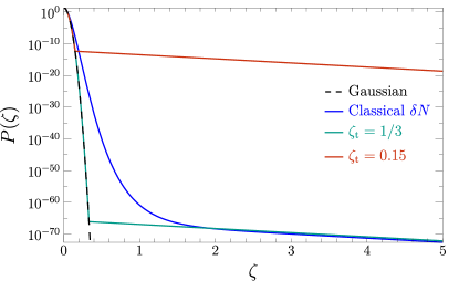
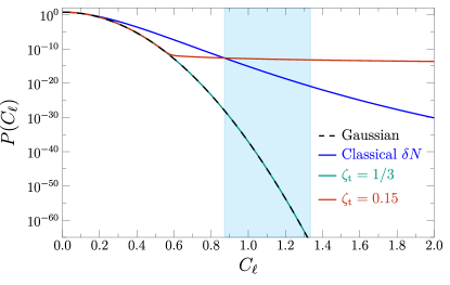
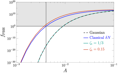
Figure 1: Comparison of the piecewise exponential and the classical USR $\delta N$ transformation. The slope, $\alpha=3$, is taken to match the classical USR $\delta N$ tail. The two values of $\zeta_{\mathrm{t}}$ are chosen to approximately match the classical USR $\delta N$ $P(\zeta)$ tail ($\zeta_{\mathrm{t}}=1/3$) and $f_{\mathrm{PBH}}$ curve ($\zeta_{\mathrm{t}}=0.15$). In the first three panels, $A\sim 4\times 10^{-3}$, for which the classical USR $\delta N$ distribution gives $f_{\mathrm{PBH}}=1$. The blue shaded region in the top right panel represents the region relevant for PBH formation. The grey shaded region in the bottom right panel indicates overproduction of PBHs ($f_{\mathrm{PBH}}>1$).

Figure 1 shows a comparison of the piecewise exponential model in eq. (26) with the Gaussian and classical USR $\delta N$ cases. We choose $\alpha=3$ in order to match the slope in the exponential tail of the classical USR $\delta N$ distribution (25). We select two values for the piecewise transition: $\zeta_{\mathrm{t}}=1/3$, to match the far tail of the classical USR $\delta N$ distribution as can be seen in the top-left panel, and $\zeta_{\mathrm{t}}=0.15$, to approximately match the $f_{\mathrm{PBH}}$ curve in the bottom-right panel. The top-right panel shows $P(C_{\mathchoice{\mathord{\lower 0.3014pt\hbox{\kern-0.3999pt\hbox{\rotatebox{10.0}{$\displaystyle\ell$}}\kern-0.3999pt}}}{\mathord{\lower 0.3014pt\hbox{\kern-0.3999pt\hbox{\rotatebox{10.0}{$\textstyle\ell$}}\kern-0.3999pt}}}{\mathord{\lower 0.3014pt\hbox{\kern-0.27992pt\hbox{\rotatebox{10.0}{$\scriptstyle\ell$}}\kern-0.27992pt}}}{\mathord{\lower 0.3014pt\hbox{\kern-0.19995pt\hbox{\rotatebox{10.0}{$\scriptscriptstyle\ell$}}\kern-0.19995pt}}}})$, calculated using eq. (20). It is clear that for $\zeta_{\mathrm{t}}=1/3$, there is no enhancement in the piecewise model over the Gaussian case, indicating that the exponential tail in the classical USR $\delta N$ model does not actually enhance the production of PBHs, with the enhancement instead coming from the transition region between $\zeta\approx 0.2$ and $1.6$ in the top left panel. This is corroborated by the $f_{\mathrm{PBH}}$ curves, where the $\zeta_{\mathrm{t}}=1/3$ case is identical to the Gaussian. It is also clear from the top right panel that the classical USR $\delta N$ model, and the piecewise model with $\zeta_{\mathrm{t}}=0.15$ chosen to produce a similar PBH enhancement, have significant support for $C_{\mathchoice{\mathord{\lower 0.3014pt\hbox{\kern-0.3999pt\hbox{\rotatebox{10.0}{$\displaystyle\ell$}}\kern-0.3999pt}}}{\mathord{\lower 0.3014pt\hbox{\kern-0.3999pt\hbox{\rotatebox{10.0}{$\textstyle\ell$}}\kern-0.3999pt}}}{\mathord{\lower 0.3014pt\hbox{\kern-0.27992pt\hbox{\rotatebox{10.0}{$\scriptstyle\ell$}}\kern-0.27992pt}}}{\mathord{\lower 0.3014pt\hbox{\kern-0.19995pt\hbox{\rotatebox{10.0}{$\scriptscriptstyle\ell$}}\kern-0.19995pt}}}}$ values larger than the cutoff of 4/3. This suggests that if type II perturbations do collapse to form PBHs, they will contribute significantly to the total abundance in these non-Gaussian models.

The bottom left panel shows the mass distribution $f(m)$, normalised by the total dark matter fraction $f_{\mathrm{PBH}}$. As expected, the Gaussian and $\zeta_{\mathrm{t}}=1/3$ distributions are identical. However, it is clear that the $\zeta_{\mathrm{t}}=0.15$ curve is significantly different, without the decaying behaviour for $m>M_{k_{*}}$. This is because the mass distribution defined in eq. (22) has a divergence at the mass corresponding to $C_{\mathchoice{\mathord{\lower 0.3014pt\hbox{\kern-0.3999pt\hbox{\rotatebox{10.0}{$\displaystyle\ell$}}\kern-0.3999pt}}}{\mathord{\lower 0.3014pt\hbox{\kern-0.3999pt\hbox{\rotatebox{10.0}{$\textstyle\ell$}}\kern-0.3999pt}}}{\mathord{\lower 0.3014pt\hbox{\kern-0.27992pt\hbox{\rotatebox{10.0}{$\scriptstyle\ell$}}\kern-0.27992pt}}}{\mathord{\lower 0.3014pt\hbox{\kern-0.19995pt\hbox{\rotatebox{10.0}{$\scriptscriptstyle\ell$}}\kern-0.19995pt}}}}=4/3$, coming from the $(1-\frac{3}{4}C_{\mathchoice{\mathord{\lower 0.3014pt\hbox{\kern-0.3999pt\hbox{\rotatebox{10.0}{$\displaystyle\ell$}}\kern-0.3999pt}}}{\mathord{\lower 0.3014pt\hbox{\kern-0.3999pt\hbox{\rotatebox{10.0}{$\textstyle\ell$}}\kern-0.3999pt}}}{\mathord{\lower 0.3014pt\hbox{\kern-0.27992pt\hbox{\rotatebox{10.0}{$\scriptstyle\ell$}}\kern-0.27992pt}}}{\mathord{\lower 0.3014pt\hbox{\kern-0.19995pt\hbox{\rotatebox{10.0}{$\scriptscriptstyle\ell$}}\kern-0.19995pt}}}})$ term in the denominator. All of the mass distributions in fig. 1 have this divergence at the right hand limit of the mass range, but it is not visible for the other curves, because $P(C_{\mathchoice{\mathord{\lower 0.3014pt\hbox{\kern-0.3999pt\hbox{\rotatebox{10.0}{$\displaystyle\ell$}}\kern-0.3999pt}}}{\mathord{\lower 0.3014pt\hbox{\kern-0.3999pt\hbox{\rotatebox{10.0}{$\textstyle\ell$}}\kern-0.3999pt}}}{\mathord{\lower 0.3014pt\hbox{\kern-0.27992pt\hbox{\rotatebox{10.0}{$\scriptstyle\ell$}}\kern-0.27992pt}}}{\mathord{\lower 0.3014pt\hbox{\kern-0.19995pt\hbox{\rotatebox{10.0}{$\scriptscriptstyle\ell$}}\kern-0.19995pt}}}})$ is decaying faster than the term in the denominator. However, for the $\zeta_{\mathrm{t}}=0.15$ case, the top-right panel shows that $P(C_{\mathchoice{\mathord{\lower 0.3014pt\hbox{\kern-0.3999pt\hbox{\rotatebox{10.0}{$\displaystyle\ell$}}\kern-0.3999pt}}}{\mathord{\lower 0.3014pt\hbox{\kern-0.3999pt\hbox{\rotatebox{10.0}{$\textstyle\ell$}}\kern-0.3999pt}}}{\mathord{\lower 0.3014pt\hbox{\kern-0.27992pt\hbox{\rotatebox{10.0}{$\scriptstyle\ell$}}\kern-0.27992pt}}}{\mathord{\lower 0.3014pt\hbox{\kern-0.19995pt\hbox{\rotatebox{10.0}{$\scriptscriptstyle\ell$}}\kern-0.19995pt}}}})$ is decaying very slowly, so does not beat the diverging term. The mass distribution $f(m)$ arising from the classical USR $\delta N$ model does decay for $m>M_{k_{*}}$, despite having a far tail slope of $\alpha=3$ in $P(\zeta)$ like the piecewise model. This is because, as stated previously, the relevant part of $P(\zeta)$ is not the far tail, but the transition, during which the effective value of $\alpha$ is significantly larger, leading to a decaying $P(C_{\mathchoice{\mathord{\lower 0.3014pt\hbox{\kern-0.3999pt\hbox{\rotatebox{10.0}{$\displaystyle\ell$}}\kern-0.3999pt}}}{\mathord{\lower 0.3014pt\hbox{\kern-0.3999pt\hbox{\rotatebox{10.0}{$\textstyle\ell$}}\kern-0.3999pt}}}{\mathord{\lower 0.3014pt\hbox{\kern-0.27992pt\hbox{\rotatebox{10.0}{$\scriptstyle\ell$}}\kern-0.27992pt}}}{\mathord{\lower 0.3014pt\hbox{\kern-0.19995pt\hbox{\rotatebox{10.0}{$\scriptscriptstyle\ell$}}\kern-0.19995pt}}}})$ and a tail in the mass distribution. It should also be noted that the critical collapse relation in eq. (21) has been used right up to $C_{\mathchoice{\mathord{\lower 0.3014pt\hbox{\kern-0.3999pt\hbox{\rotatebox{10.0}{$\displaystyle\ell$}}\kern-0.3999pt}}}{\mathord{\lower 0.3014pt\hbox{\kern-0.3999pt\hbox{\rotatebox{10.0}{$\textstyle\ell$}}\kern-0.3999pt}}}{\mathord{\lower 0.3014pt\hbox{\kern-0.27992pt\hbox{\rotatebox{10.0}{$\scriptstyle\ell$}}\kern-0.27992pt}}}{\mathord{\lower 0.3014pt\hbox{\kern-0.19995pt\hbox{\rotatebox{10.0}{$\scriptscriptstyle\ell$}}\kern-0.19995pt}}}}=4/3$, but is expected to break down before this point [52].

Figure 2 shows the effect of changing the piecewise transition point $\zeta_{\mathrm{t}}$ and exponential slope $\alpha$ in eq. (26) on the total PBH abundance $f_{\mathrm{PBH}}$ and the mass distribution $f(m)$. As in fig. 1, the largest values of $\zeta_{\mathrm{t}}$ provide no enhancement over the Gaussian PDF except at the highest amplitudes, for which $f_{\mathrm{PBH}}\gg 1$. For smaller values of $\zeta_{\mathrm{t}}$, the exponential tail does provide a significant enhancement over the Gaussian case, greatly reducing the amplitude required for $f_{\mathrm{PBH}}=1$. In contrast, changing $\alpha$ only moves the $f_{\mathrm{PBH}}$ curve by a (relatively) small amount, e.g. by factors of $10$ rather than the $10^{10}$ coming from changing $\zeta_{\text{t}}$. The steeper values of $\alpha$ are suppressed compared to the shallower slopes, as expected. For large amplitudes, $f_{\mathrm{PBH}}$ is suppressed (even compared to the Gaussian). This suppression comes from the normalisation of $P(\zeta)$ when including a large tail. The details of this suppression are unimportant, since they correspond to $f_{\mathrm{PBH}}\gg 1$ and so these power spectrum amplitudes are disallowed anyway for PBH masses that survive to the present day.

In the bottom two panels we can see the effect of changing $\zeta_{\mathrm{t}}$ and $\alpha$ on the mass distribution $f(m)$. For $\zeta_{\mathrm{t}}$, there are three cases that are visible. The $\zeta_{\mathrm{t}}=0.3$ curve lies on top of the Gaussian, as for the $\zeta_{\mathrm{t}}=1/3$ case in fig. 1. For $\zeta_{\mathrm{t}}=0.25$, the function $f(m)$ starts to decrease for $m>M_{k_{*}}$ as $P(C_{\mathchoice{\mathord{\lower 0.3014pt\hbox{\kern-0.3999pt\hbox{\rotatebox{10.0}{$\displaystyle\ell$}}\kern-0.3999pt}}}{\mathord{\lower 0.3014pt\hbox{\kern-0.3999pt\hbox{\rotatebox{10.0}{$\textstyle\ell$}}\kern-0.3999pt}}}{\mathord{\lower 0.3014pt\hbox{\kern-0.27992pt\hbox{\rotatebox{10.0}{$\scriptstyle\ell$}}\kern-0.27992pt}}}{\mathord{\lower 0.3014pt\hbox{\kern-0.19995pt\hbox{\rotatebox{10.0}{$\scriptscriptstyle\ell$}}\kern-0.19995pt}}}})$ decreases, before growing again due to the diverging term discussed previously. Finally, all values of $\zeta_{\mathrm{t}}$ smaller than 0.25 show no drop-off for $m>M_{k_{*}}$, instead being dominated by the diverging factor. Comparing the $f_{\mathrm{PBH}}$ and $f(m)$ plots for varying $\zeta_{\mathrm{t}}$, it seems clear that the amount of non-Gaussianity required to significantly reduce the power spectrum amplitude corresponding to a fixed $f_{\mathrm{PBH}}$ will also have a large impact on the mass distribution. This is important in the case of evading tight constraints such as those from $\mu$-distortions [53]. The right panel shows that, as with $f_{\mathrm{PBH}}$, the mass distribution is less affected by $\alpha$ than $\zeta_{\mathrm{t}}$, with all the curves appearing basically identical. This is consistent with the conclusion from fig. 1 that the transition regime provides the enhancement, rather than the far tail.

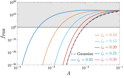
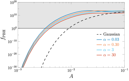
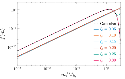
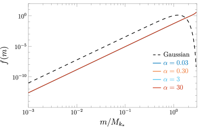
Figure 2: Comparison of $f_{\mathrm{PBH}}(A)$ (top) and $f(m)$ (bottom) for different values of the piecewise distribution parameters $\zeta_{\mathrm{t}}$ and $\alpha$, with $\alpha=3$ (left) and $\zeta_{\mathrm{t}}=0.15$ (right). The grey shaded region in the top row indicates overproduction of PBHs ($f_{\mathrm{PBH}}>1$). The mass distributions $f(m)$ in the bottom row are normalised to $f_{\mathrm{PBH}}=1$.

Table 1: Approximate values of $\nu_{t}=\zeta_{\mathrm{t}}/\sqrt{\Sigma_{YY}}$ and $P(\zeta_{\mathrm{t}})$ required for a specific $f_{\mathrm{PBH}}$, with a given $\alpha$. There is a linear relationship between $P(\zeta_{\mathrm{t}})$ and $f_{\mathrm{PBH}}$ for constant $\alpha$, and an inverse linear relationship between $f_{\mathrm{PBH}}$ and $\alpha$ for fixed $\nu_{t}$, which comes about from the integration of the far tail exponential behaviour.

$\alpha$	$\nu_{t}$	$P(\zeta_{\mathrm{t}})$	$f_{\mathrm{PBH}}$
3	8.2	$10^{-10}$	1
	10.7	$10^{-20}$	$10^{-10}$
0.3	8.2	$10^{-10}$	10
30	8.2	$10^{-10}$	$10^{-1}$

IV Conclusions

In this work, we have developed a non-perturbative treatment of primordial non-Gaussianity, when it is of a generalised local type, and applied it to the formation of primordial black holes by relating the curvature perturbation $\zeta$ to the compaction function $C$. A non-perturbative method is essential when considering non-Gaussianities that are not described by the usual $f_{\mathrm{NL}}$ expansion, such as those appearing in the stochastic treatment of inflation. Our method assumes there exists a generalised local transformation from a Gaussian field, $\zeta(\zeta_{\mathrm{G}},r)$, and it remains to be seen whether this is a good description of the non-Gaussianity generated by stochastic diffusion. Previous works have used the classical USR $\delta N$ relation for a local-type non-Gaussian $\zeta(\zeta_{\mathrm{G}})$ with a PDF that smoothly transitions from a Gaussian to an exponential tail. By comparing to a simple piecewise model with a sudden transition between a Gaussian and an exponential with the same slope, we have shown that the enhanced PBH formation in the classical USR $\delta N$ model is due to the transition regime, rather than the far tail. Additionally, we have examined the transition value, $\zeta_{\mathrm{t}}$, required for $f_{\mathrm{PBH}}=1$ using our piecewise model. We find that $\nu_{t}=\zeta_{\mathrm{t}}/\sqrt{\Sigma_{YY}}$ is approximately independent of the peak amplitude of the Gaussian power spectrum, $A$, for fixed $f_{\mathrm{PBH}}$ and $\alpha$. We also see a linear relationship between $P(\zeta_{\mathrm{t}})$ and $f_{\mathrm{PBH}}$, and when changing the exponential slope $\alpha$ we find an inverse linear relation between $f_{\mathrm{PBH}}$ and $\alpha$, see table 1. We also show that, for sufficiently shallow exponential tail slopes, the PBH mass distribution is dominated by a diverging term for high masses. This effect will be important when significant non-Gaussianity is required to reduce the power spectrum amplitude by orders of magnitude at fixed $f_{\mathrm{PBH}}$, e.g. to evade the $\mu$-distortion constraints for supermassive PBHs.

Note added

During the writing up of this paper, Ref. [54] appeared on the arXiv. The authors utilise the same mechanism of writing $\zeta$ in terms of $\zeta_{\mathrm{G}}$ and applying the product rule to the derivative in the compaction function, but restrict themselves to local transformations $\zeta(\zeta_{\mathrm{G}})$, rather than allowing $P(\zeta)$ to be arbitrary.

References

- [1] Ya. B. Zel’dovich and I. D. Novikov, The Hypothesis of Cores Retarded during Expansion and the Hot Cosmological Model, Soviet Astronomy 10(4) (1967) 602.
- [2] S. Hawking, Gravitationally Collapsed Objects of Very Low Mass, Monthly Notices of the Royal Astronomical Society 152(1) (1971) 75.
- [3] B. J. Carr and S. W. Hawking, Black Holes in the Early Universe, Monthly Notices of the Royal Astronomical Society 168(2) (1974) 399.
- [4] B. Carr, K. Kohri, Y. Sendouda and J. Yokoyama, Constraints on primordial black holes, Reports on Progress in Physics 84(11) (2021) 116902 [2002.12778].
- [5] S. Bird et al., Did LIGO Detect Dark Matter?, Physical Review Letters 116(20) (2016) 201301 [1603.00464].
- [6] M. Sasaki, T. Suyama, T. Tanaka and S. Yokoyama, Primordial Black Hole Scenario for the Gravitational-Wave Event GW150914, Physical Review Letters 117(6) (2016) 061101 [1603.08338].
- [7] S. Clesse and J. García-Bellido, The clustering of massive Primordial Black Holes as Dark Matter: Measuring their mass distribution with advanced LIGO, Physics of the Dark Universe 15 (2017) 142 [1603.05234].
- [8] A. D. Gow, C. T. Byrnes, A. Hall and J. A. Peacock, Primordial black hole merger rates: distributions for multiple LIGO observables, Journal of Cosmology and Astroparticle Physics 2020(01) (2020) 031 [1911.12685].
- [9] G. Franciolini et al., Searching for a subpopulation of primordial black holes in LIGO-Virgo gravitational-wave data, Physical Review D 105(8) (2022) 083526 [2105.03349].
- [10] Planck collaboration, Planck 2018 results. VI. Cosmological parameters, Astronomy & Astrophysics 641 (2020) A6 [1807.06209].
- [11] A. D. Gow, C. T. Byrnes, P. S. Cole and S. Young, The power spectrum on small scales: robust constraints and comparing PBH methodologies, Journal of Cosmology and Astroparticle Physics 2021(02) (2021) 002 [2008.03289].
- [12] J. S. Bullock and J. R. Primack, Non-Gaussian fluctuations and primordial black holes from inflation, Physical Review D 55(12) (1997) 7423 [astro-ph/9611106].
- [13] S. Young, D. Regan and C. T. Byrnes, Influence of large local and non-local bispectra on primordial black hole abundance, Journal of Cosmology and Astroparticle Physics 2016(02) (2016) 029 [1512.07224].
- [14] C.-M. Yoo, J.-O. Gong and S. Yokoyama, Abundance of primordial black holes with local non-Gaussianity in peak theory, Journal of Cosmology and Astroparticle Physics 2019(09) (2019) 033 [1906.06790].
- [15] G. A. Palma, B. Scheihing Hitschfeld and S. Sypsas, Non-Gaussian CMB and LSS statistics beyond polyspectra, Journal of Cosmology and Astroparticle Physics 2020(02) (2020) 027 [1907.05332].
- [16] M. Taoso and A. Urbano, Non-gaussianities for primordial black hole formation, Journal of Cosmology and Astroparticle Physics 2021(08) (2021) 016 [2102.03610].
- [17] S. Young, Peaks and primordial black holes: the effect of non-gaussianity, Journal of Cosmology and Astroparticle Physics 2022(05) (2022) 037 [2201.13345].
- [18] D. H. Lyth and Y. Rodríguez, Inflationary Prediction for Primordial Non-Gaussianity, Physical Review Letters 95(12) (2005) 121302 [astro-ph/0504045].
- [19] T. Fujita, M. Kawasaki, Y. Tada and T. Takesako, A new algorithm for calculating the curvature perturbations in stochastic inflation, Journal of Cosmology and Astroparticle Physics 2013(12) (2013) 036 [1308.4754].
- [20] V. Vennin and A. A. Starobinsky, Correlation functions in stochastic inflation, The European Physical Journal C 75 (2015) 413 [1506.04732].
- [21] C. Pattison, V. Vennin, H. Assadullahi and D. Wands, Quantum diffusion during inflation and primordial black holes, Journal of Cosmology and Astroparticle Physics 2017(10) (2017) 046 [1707.00537].
- [22] J. M. Ezquiaga, J. García-Bellido and V. Vennin, The exponential tail of inflationary fluctuations: consequences for primordial black holes, Journal of Cosmology and Astroparticle Physics 2020(03) (2020) 029 [1912.05399].
- [23] V. Vennin, Stochastic inflation and primordial black holes, Habilitation thesis, (2020) [2009.08715].
- [24] D. G. Figueroa, S. Raatikainen, S. Räsänen and E. Tomberg, Non-Gaussian Tail of the Curvature Perturbation in Stochastic Ultraslow-Roll Inflation: Implications for Primordial Black Hole Production, Physical Review Letters 127(10) (2021) 101302 [2012.06551].
- [25] K. Ando and V. Vennin, Power spectrum in stochastic inflation, Journal of Cosmology and Astroparticle Physics 2021(04) (2021) 057 [2012.02031].
- [26] C. Pattison, V. Vennin, D. Wands and H. Assadullahi, Ultra-slow-roll inflation with quantum diffusion, Journal of Cosmology and Astroparticle Physics 2021(04) (2021) 080 [2101.05741].
- [27] G. Rigopoulos and A. Wilkins, Inflation is always semi-classical: diffusion domination overproduces Primordial Black Holes, Journal of Cosmology and Astroparticle Physics 2021(12) (2021) 027 [2107.05317].
- [28] Y. Tada and V. Vennin, Statistics of coarse-grained cosmological fields in stochastic inflation, Journal of Cosmology and Astroparticle Physics 2022(02) (2022) 021 [2111.15280].
- [29] J. H. P. Jackson et al., Numerical simulations of stochastic inflation using importance sampling, Journal of Cosmology and Astroparticle Physics 2022(10) (2022) 067 [2206.11234].
- [30] C. Animali and V. Vennin, Primordial black holes from stochastic tunnelling, Journal of Cosmology and Astroparticle Physics 2023(02) (2023) 043 [2210.03812].
- [31] G. Panagopoulos and E. Silverstein, Primordial Black Holes from non-Gaussian tails, (2019) [1906.02827].
- [32] A. Achúcarro, S. Céspedes, A.-C. Davis and G. A. Palma, The hand-made tail: non-perturbative tails from multifield inflation, Journal of High Energy Physics 2022(05) (2022) 052 [2112.14712].
- [33] Y.-F. Cai et al., Highly non-Gaussian tails and primordial black holes from single-field inflation, Journal of Cosmology and Astroparticle Physics 2022(12) (2022) 034 [2207.11910].
- [34] M. Shibata and M. Sasaki, Black hole formation in the Friedmann universe: Formulation and computation in numerical relativity, Physical Review D 60(8) (1999) 084002 [gr-qc/9905064].
- [35] T. Harada, C.-M. Yoo, T. Nakama and Y. Koga, Cosmological long-wavelength solutions and primordial black hole formation, Physical Review D 91(8) (2015) 084057 [1503.03934].
- [36] M. Kopp, S. Hofmann and J. Weller, Separate universes do not constrain primordial black hole formation, Physical Review D 83(12) (2011) 124025 [1012.4369].
- [37] V. De Luca and A. Riotto, A note on the abundance of primordial black holes: Use and misuse of the metric curvature perturbation, Physics Letters B 828 (2022) 137035 [2201.09008].
- [38] M. Biagetti et al., The formation probability of primordial black holes, Physics Letters B 820 (2021) 136602 [2105.07810].
- [39] N. Kitajima, Y. Tada, S. Yokoyama and C.-M. Yoo, Primordial black holes in peak theory with a non-Gaussian tail, Journal of Cosmology and Astroparticle Physics 2021(10) (2021) 053 [2109.00791].
- [40] M. W. Choptuik, Universality and scaling in gravitational collapse of a massless scalar field, Physical Review Letters 70(1) (1993) 9.
- [41] C. R. Evans and J. S. Coleman, Critical phenomena and self-similarity in the gravitational collapse of radiation fluid, Physical Review Letters 72(12) (1994) 1782 [gr-qc/9402041].
- [42] J. C. Niemeyer and K. Jedamzik, Near-Critical Gravitational Collapse and the Initial Mass Function of Primordial Black Holes, Physical Review Letters 80(25) (1998) 5481 [astro-ph/9709072].
- [43] I. Musco, Threshold for primordial black holes: Dependence on the shape of the cosmological perturbations, Physical Review D 100(12) (2019) 123524 [1809.02127].
- [44] S. Young, The primordial black hole formation criterion re-examined: Parametrisation, timing and the choice of window function, International Journal of Modern Physics D 29(02) (2019) 2030002 [1905.01230].
- [45] C. Germani and I. Musco, Abundance of Primordial Black Holes Depends on the Shape of the Inflationary Power Spectrum, Physical Review Letters 122(14) (2019) 141302 [1805.04087].
- [46] C. Germani and R. K. Sheth, Nonlinear statistics of primordial black holes from Gaussian curvature perturbations, Physical Review D 101(6) (2020) 063520 [1912.07072].
- [47] A. Escrivà, C. Germani and R. K. Sheth, Analytical thresholds for black hole formation in general cosmological backgrounds, Journal of Cosmology and Astroparticle Physics 2021(01) (2021) 030 [2007.05564].
- [48] I. Musco, V. De Luca, G. Franciolini and A. Riotto, Threshold for primordial black holes. II. A simple analytic prescription, Physical Review D 103(6) (2021) 063538 [2011.03014].
- [49] Y.-F. Cai et al., Revisiting non-Gaussianity from non-attractor inflation models, Journal of Cosmology and Astroparticle Physics 2018(05) (2018) 012 [1712.09998].
- [50] V. Atal, J. Garriga and A. Marcos-Caballero, Primordial black hole formation with non-Gaussian curvature perturbations, Journal of Cosmology and Astroparticle Physics 2019(09) (2019) 073 [1905.13202].
- [51] S. Pi and M. Sasaki, Primordial Black Hole Formation in Non-Minimal Curvaton Scenario, (2021) [2112.12680].
- [52] A. Escrivà, Simulation of primordial black hole formation using pseudo-spectral methods, Physics of the Dark Universe 27 (2020) 100466 [1907.13065].
- [53] J. Chluba, A. L. Erickcek and I. Ben-Dayan, PROBING THE INFLATON: SMALL-SCALE POWER SPECTRUM CONSTRAINTS FROM MEASUREMENTS OF THE COSMIC MICROWAVE BACKGROUND ENERGY SPECTRUM, The Astrophysical Journal 758(2) (2012) 76 [1203.2681].
- [54] G. Ferrante, G. Franciolini, A. J. Iovino and A. Urbano, Primordial non-Gaussianity up to all orders: Theoretical aspects and implications for primordial black hole models, Phys. Rev. D 107(4) (2023) 043520 [2211.01728].