Pruning Very Deep Neural Network Channels for Efficient Inference

Abstract

In this paper, we introduce a new channel pruning method to accelerate very deep convolutional neural networks. Given a trained CNN model, we propose an iterative two-step algorithm to effectively prune each layer, by a LASSO regression based channel selection and least square reconstruction. We further generalize this algorithm to multi-layer and multi-branch cases. Our method reduces the accumulated error and enhances the compatibility with various architectures. Our pruned VGG-16 achieves the state-of-the-art results by $5\times$ speed-up along with only 0.3% increase of error. More importantly, our method is able to accelerate modern networks like ResNet, Xception and suffers only 1.4%, 1.0% accuracy loss under $2\times$ speed-up respectively, which is significant. Our code has been made publicly available.

1 Introduction

Recently, convolutional neural networks (CNNs) are widely used on embed systems like smartphones and self-driving cars. The general trend since the past few years has been that the networks have grown deeper, with an overall increase in the number of parameters and convolution operations. Efficient inference is becoming more and more crucial for CNNs [1]. CNN acceleration works fall into three categories: optimized implementation (e.g., FFT [2]), quantization (e.g., BinaryNet [3]), and structured simplification that convert a CNN into compact one [4]. This work focuses on the last one since it directly deals with the over-parameterization of CNNs.

Structured simplification mainly involves: tensor factorization [4], sparse connection [5], and channel pruning [6]. Tensor factorization factorizes a convolutional layer into several efficient ones (Fig. 1(c)). However, feature map width (number of channels) could not be reduced, which makes it difficult to decompose $1\times 1$ convolutional layers favored by modern networks (e.g., GoogleNet [7], ResNet [8], Xception [9]). This type of method also introduces extra computation overhead. Sparse connection deactivates connections between neurons or channels (Fig. 1(b)). Though it is able to achieve high theoretical ,/the sparse convolutional layers have an ”irregular” shape which is not implementation-friendly. In contrast, channel pruning directly reduces feature map width, which shrinks a network into thinner one, as shown in Fig. 1(d). It is efficient on both CPU and GPU because no special implementation is required.

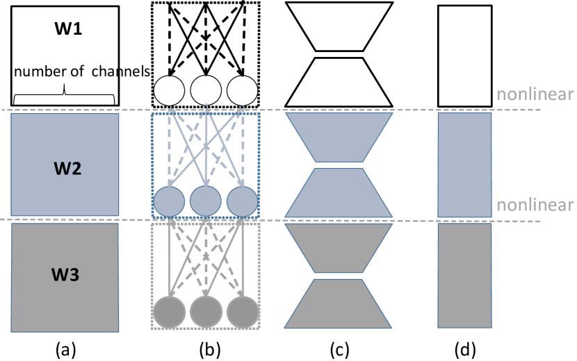
Figure 1: Structured simplification methods that accelerate CNNs: (a) a network with 3 conv layers. (b) sparse connection deactivates some connections between channels. (c) tensor factorization factorizes a convolutional layer into several pieces. (d) channel pruning reduces number of channels in each layer (focus of this paper).

Channel pruning is simple but challenging because removing channels in one layer might dramatically change the input of the following layer. Recently, training-based channel pruning works [10, 6] have focused on imposing the sparse constraint on weights during training, which could adaptively determine hyper-parameters. However, training from scratch is very costly, and results for very deep CNNs on ImageNet have rarely been reported. Inference-time attempts [11, 12] have focused on analysis of the importance of individual weight. The reported  /is very limited.

This work is initially inspired by Net2widerNet [13], which could easily explore new wider networks specification of the same architecture. It makes a convolutional layer wider by creating several copies of itself, calling each copy so that the output feature map is unchanged. It’s nature to ask: Is it possible to convert a net to thinner net of the same architecture without losing accuracy? If we regard each feature map as a vector, then all feature maps form a vector space. The inverse operation of Net2widerNet discussed above is to find a set of base feature vectors and use them to represent other feature vectors, in order to reconstruct the original feature map space.

In this paper, we propose a new inference-time approach for channel pruning, utilizing inter-channel redundancy. Inspired by tensor factorization improvement by feature maps reconstruction [14], instead of pruning according to filter weights magnitude [11, 15], we fully exploit redundancy inter feature maps. Instead of recovering performance with finetuning [5, 11, 15], we propose to reconstruct output after pruning each layer. Specifically, given a trained CNN model, pruning each layer is achieved by minimizing reconstruction error on its output feature maps, as shown in Fig. 2.

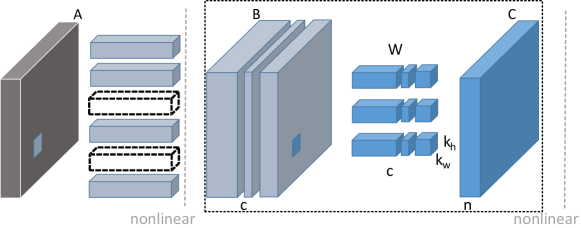
Figure 2: Channel pruning for accelerating a convolutional layer. We aim to reduce the number of channels of feature map and minimize the reconstruction error on feature map C. Our optimization algorithm (Sec. 3.1) performs within the dotted box, which does not involve nonlinearity. This figure illustrates the situation that two channels are pruned for feature map B. Thus corresponding channels of filters $\mathrm{W}$ can be removed. Furthermore, even though not directly optimized by our algorithm, the corresponding filters in the previous layer can also be removed (marked by dotted filters). $c,n$: number of channels for feature maps B and C, $k_{h}\times k_{w}$: kernel size.

We solve this minimization problem by two alternative steps: channels selection and feature map reconstruction. In one step, we figure out the most representative channels, and prune redundant ones, based on LASSO regression. In the other step, we reconstruct the outputs with remaining channels with linear least squares. We alternatively take two steps. Further, we approximate the network layer-by-layer, with accumulated error accounted. We also discuss methodologies to prune multi-branch networks (e.g., ResNet [8], Xception [9]).

We demonstrate the superior accuracy of our approach over other recent pruning techniques [16, 15, 17, 18]. For VGG-16, we achieve $4\times$ acceleration, with only 1.0% increase of top-5 error. Combined with tensor factorization, we reach $5\times$ acceleration but merely suffer 0.3% increase of error, which outperforms previous state-of-the-arts. We further speed up ResNet-50 and Xception-50 by $2\times$ with only 1.4%, 1.0% accuracy loss respectively. Code has been made publicly available .

A preliminary version of this manuscript has been accepted to a conference [19]. This manuscript extends the initial version from several aspects to strengthen our approach:

1. We investigated inter-channel redundancy in each layer, and better analysis it for pruning.

2. We present filter-wise pruning, which has compelling acceleration performance for a single layer.

3. We demonstrated compelling VGG-16 acceleration Top-1 results which outperform its original model.

2 Related Work

There has been a significant amount of work on accelerating CNNs [20], starting from brain damage [21, 22]. Many of them fall into three categories: optimized implementation [23], quantization [24], and structured simplification [4].

Optimized implementation based methods [25, 2, 26, 23] accelerate convolution, with special convolution algorithms like FFT [2]. Quantization [3, 24, 27] reduces floating point computational complexity.

Sparse connection eliminates connections between neurons [5, 28, 29, 30, 31, 32, 33]. [34] prunes connections based on weights magnitude. [35] could accelerate fully connected layers up to $50\times$. However, in practice, the actual speed-up may be very related to implementation.

Tensor factorization [4, 36, 37, 38, 39] decompose weights into several pieces. [40, 41, 42] accelerate fully connected layers with truncated SVD. [14] factorize a layer into $3\times 3$ and $1\times 1$ combination, driven by feature map redundancy.

Channel pruning removes redundant channels on feature maps. There are several training-based approaches [43]. [10, 6, 44] regularize networks to improve accuracy. Channel-wise SSL [6] reaches high compression ratio for first few conv layers of LeNet [45] and AlexNet [46]. [44] could work well for fully connected layers. However, training-based approaches are more costly, and their effectiveness on very deep networks on large datasets is rarely exploited. Inference-time channel pruning is challenging, as reported by previous works [47, 48]. Recently, AMC [49] improves our approach by learning speed-up ratio with reinforcement learning.

Some works [50, 51, 52] focus on model size compression, which mainly operate the fully connected layers. Data-free approaches [11, 12] results for  /(e.g., $5\times$) have not been reported, and requires long retraining procedure. [12] select channels via over 100 random trials. However, it needs a long time to evaluate each trial on a deep network, which makes it infeasible to work on very deep models and large datasets. [11] is even worse than naive solution from our observation sometimes (Sec. 4.1.1).

3 Approach

In this section, we first propose a channel pruning algorithm for a single layer, then generalize this approach to multiple layers or the whole model. Furthermore, we discuss variants of our approach for multi-branch networks.

3.1 Formulation

Figure 2 illustrates our channel pruning algorithm for a single convolutional layer. We aim to reduce the number of channels of feature map B while maintaining outputs in feature map C. Once channels are pruned, we can remove corresponding channels of the filters that take these channels as input. Also, filters that produce these channels can also be removed. It is clear that channel pruning involves two key points. The first is channel selection since we need to select proper channel combination to maintain as much information. The second is reconstruction. We need to reconstruct the following feature maps using the selected channels.

Motivated by this, we propose an iterative two-step algorithm:

1. In one step, we aim to select most representative channels. Since an exhaustive search is infeasible even for small networks, we come up with a LASSO regression based method to figure out representative channels and prune redundant ones.

2. In the other step, we reconstruct the outputs with remaining channels with linear least squares.

We alternatively take two steps.

Formally, to prune a feature map B with $c$ channels, we consider applying $n\times c\times k_{h}\times k_{w}$ convolutional filters $\mathrm{W}$ on $N\times c\times k_{h}\times k_{w}$ input volumes $\mathrm{X}$ sampled from this feature map, which produces $N\times n$ output matrix $\mathrm{Y}$ from feature map C. Here, $N$ is the number of samples, $n$ is the number of output channels, and $k_{h},k_{w}$ are the kernel size. For simple representation, bias term is not included in our formulation. To prune the input channels from $c$ to desired $c^{\prime}$ ($0\leq c^{\prime}\leq c$), while minimizing reconstruction error, we formulate our problem as follow:

$$\operatorname*{arg\,min}_{\boldsymbol{\beta},\mathrm{W}}\frac{1}{2N}\left\lVert\mathrm{Y}-\sum_{i=1}^{c}\beta_{i}\mathrm{X_{i}}\mathrm{W_{i}}^{\top}\right\rVert^{2}_{F}$$ (1)

$$\text{subject to}\left\lVert\boldsymbol{\beta}\right\rVert_{0}\leq c^{\prime}$$

$\left\lVert\cdot\right\rVert_{F}$ is Frobenius norm. $\mathrm{X_{i}}$ is $N\times k_{h}k_{w}$ matrix sliced from $i$th channel of input volumes $\mathrm{X}$, $i=1,...,c$. $\mathrm{W_{i}}$ is $n\times k_{h}k_{w}$ filter weights sliced from $i$th channel of $\mathrm{W}$. $\boldsymbol{\beta}$ is coefficient vector of length $c$ for channel selection, and $\beta_{i}$ ($i$th entry of $\boldsymbol{\beta}$) is a scalar mask to $i$th channel (i.e. to drop the whole channel or not). Notice that, if $\beta_{i}=0$, $\mathrm{X_{i}}$ will be no longer useful, which could be safely pruned from feature map B. $\mathrm{W_{i}}$ could also be removed. $c^{\prime}$ is the number of retained channels, which is manually set as it can be calculated from the desired speed-up ratio. For whole-model speed-up (i.e. Section 4.1.2), given the overall speed-up, we first assign speed-up ratio for each layer then calculate each $c^{\prime}$.

3.2 Optimization

Solving this $\ell_{0}$ minimization problem in Eqn. 1 is NP-hard. Therefore, we relax the $\ell_{0}$ to $\ell_{1}$ regularization:

$$\operatorname*{arg\,min}_{\boldsymbol{\beta},\mathrm{W}}\frac{1}{2N}\left\lVert\mathrm{Y}-\sum_{i=1}^{c}\beta_{i}\mathrm{X_{i}}\mathrm{W_{i}}^{\top}\right\rVert^{2}_{F}+\lambda\left\lVert\boldsymbol{\beta}\right\rVert_{1}$$ (2)

$$\text{subject to}\left\lVert\boldsymbol{\beta}\right\rVert_{0}\leq c^{\prime},\forall i\left\lVert\mathrm{W_{i}}\right\rVert_{F}=1$$

$\lambda$ is a penalty coefficient. By increasing $\lambda$, there will be more zero terms in $\boldsymbol{\beta}$ and one can get higher ./We also add a constraint $\forall i\left\lVert\mathrm{W_{i}}\right\rVert_{F}=1$ to this formulation to avoid trivial solution.

Now we solve this problem in two folds. First, we fix $\mathrm{W}$, solve $\boldsymbol{\beta}$ for channel selection. Second, we fix $\boldsymbol{\beta}$, solve $\mathrm{W}$ to reconstruct error.

3.2.1 (i) The subproblem of $\boldsymbol{\beta}$

In this case, $\mathrm{W}$ is fixed. We solve $\boldsymbol{\beta}$ for channel selection. This problem can be solved by LASSO regression [53, 54], which is widely used for model selection.

$$\hat{\boldsymbol{\beta}}^{LASSO}(\lambda)=\operatorname*{arg\,min}_{\boldsymbol{\beta}}\frac{1}{2N}\left\lVert\mathrm{Y}-\sum_{i=1}^{c}\beta_{i}\mathrm{Z_{i}}\right\rVert_{F}^{2}+\lambda\left\lVert\boldsymbol{\beta}\right\rVert_{1}$$ (3)

$$\text{subject to}\left\lVert\boldsymbol{\beta}\right\rVert_{0}\leq c^{\prime}$$

Here $\mathrm{Z_{i}}=\mathrm{X_{i}}\mathrm{W_{i}}^{\top}$ (size $N\times n$). We will ignore $i$th channels if $\beta_{i}=0$.

3.2.2 (ii) The subproblem of $\mathrm{W}$

In this case, $\boldsymbol{\beta}$ is fixed. We utilize the selected channels to minimize reconstruction error. We can find optimized solution by least squares:

$$\operatorname*{arg\,min}_{\mathrm{W^{\prime}}}\left\lVert\mathrm{Y}-\mathrm{X^{\prime}}(\mathrm{W^{\prime}})^{\top}\right\rVert_{F}^{2}$$ (4)

Here $\mathrm{X^{\prime}}=[\beta_{1}\mathrm{X_{1}}\;\beta_{2}\mathrm{X_{2}}\;...\;\beta_{i}\mathrm{X_{i}}\;...\;\beta_{c}\mathrm{X_{c}}]$ (size $N\times ck_{h}k_{w}$). $\mathrm{W^{\prime}}$ is $n\times ck_{h}k_{w}$ reshaped $\mathrm{W}$, $\mathrm{W^{\prime}}=[\mathrm{W_{1}}\;\mathrm{W_{2}}\;...\;\mathrm{W_{i}}\;...\;\mathrm{W_{c}}]$. After obtained result $\mathrm{W^{\prime}}$, it is reshaped back to $\mathrm{W}$. Then we assign $\beta_{i}\leftarrow\beta_{i}\left\lVert\mathrm{W_{i}}\right\rVert_{F},\mathrm{W_{i}}\leftarrow\mathrm{W_{i}}/\left\lVert\mathrm{W_{i}}\right\rVert_{F}$. Constrain $\forall i\left\lVert\mathrm{W_{i}}\right\rVert_{F}=1$ satisfies.

We alternatively optimize (i) and (ii). In the beginning, $\mathrm{W}$ is initialized from the trained model, $\lambda=0$, namely no penalty, and $\left\lVert\boldsymbol{\beta}\right\rVert_{0}=c$. We gradually increase $\lambda$. For each change of $\lambda$, we iterate these two steps until $\left\lVert\boldsymbol{\beta}\right\rVert_{0}$ is stable. After $\left\lVert\boldsymbol{\beta}\right\rVert_{0}\leq c^{\prime}$ satisfies, we obtain the final solution $\mathrm{W}$ from $\{\beta_{i}\mathrm{W_{i}}\}$. In practice, we found that the two steps iteration is time consuming. So we apply (i) multiple times until $\left\lVert\boldsymbol{\beta}\right\rVert_{0}\leq c^{\prime}$ satisfies. Then apply (ii) just once, to obtain the final result. From our observation, this result is comparable with two steps iteration’s result. Therefore, in the following experiments, we adopt this approach for efficiency.

3.2.3 Discussion

Some recent works [6, 10, 5] (though training based) also introduce $\ell_{1}$-norm or LASSO. However, we must emphasize that we use different formulations. Many of them introduced sparsity regularization into training loss, instead of explicitly solving LASSO. Other work [10] solved LASSO, while feature maps or data were not considered during optimization.

Because of these differences, our approach could be applied at inference time.

3.3 Whole Model Pruning

Inspired by [14], we apply our approach layer by layer sequentially. For each layer, we obtain input volumes from the current input feature map, and output volumes from the output feature map of the un-pruned model. This could be formalized as:

$$\operatorname*{arg\,min}_{\boldsymbol{\beta},\mathrm{W}}\frac{1}{2N}\left\lVert\mathrm{Y}^{\prime}-\sum_{i=1}^{c}\beta_{i}\mathrm{X_{i}}\mathrm{W_{i}}^{\top}\right\rVert^{2}_{F}$$ (5)

$$\text{subject to}\left\lVert\boldsymbol{\beta}\right\rVert_{0}\leq c^{\prime}$$

Different from Eqn. 1, $\mathrm{Y}$ is replaced by $\mathrm{Y}^{\prime}$, which is from feature map of the original model. Therefore, the accumulated error could be accounted during sequential pruning.

3.4 Pruning Multi-Branch Networks

The whole model pruning discussed above is enough for single-branch networks like LeNet [45], AlexNet [46] and VGG Nets [55]. However, it is insufficient for multi-branch networks like GoogLeNet [7] and ResNet [8]. We mainly focus on pruning the widely used residual structure (e.g., ResNet [8], Xception [9]). Given a residual block shown in Figure 3 (left), the input bifurcates into the shortcut and the residual branch. On the residual branch, there are several convolutional layers (e.g., 3 convolutional layers which have spatial size of $1\times 1,3\times 3,1\times 1$, Figure 3, left). Other layers except the first and last layer can be pruned as is described previously. For the first layer, the challenge is that the large input feature map width (for ResNet, four times of its output) can’t be easily pruned since it is shared with the shortcut. For the last layer, accumulated error from the shortcut is hard to be recovered, since there’s no parameter on the shortcut. To address these challenges, we propose several variants of our approach as follows.

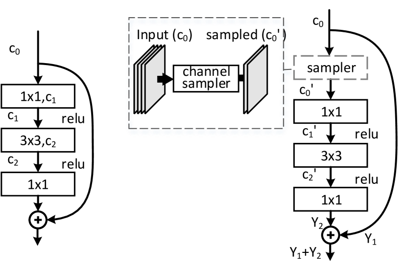
Figure 3: Illustration of multi-branch enhancement for residual block. Left: original residual block. Right: pruned residual block with enhancement, $\mathrm{c_{x}}$ denotes the feature map width. Input channels of the first convolutional layer are sampled, so that the large input feature map width could be reduced. As for the last layer, rather than approximate $\mathrm{Y}_{2}$, we try to approximate $\mathrm{Y}_{1}+\mathrm{Y}_{2}$ directly (Sec. 3 Last layer of residual branch).

3.4.1 Last layer of residual branch

Shown in Figure 3, the output layer of a residual block consists of two inputs: feature map $\mathrm{Y}_{1}$ and $\mathrm{Y}_{2}$ from the shortcut and residual branch. We aim to recover $\mathrm{Y}_{1}+\mathrm{Y}_{2}$ for this block. Here, $\mathrm{Y}_{1},\mathrm{Y}_{2}$ are the original feature maps before pruning. $\mathrm{Y}_{2}$ could be approximated as in Eqn. 1. However, shortcut branch is parameter-free, then $\mathrm{Y}_{1}$ could not be recovered directly. To compensate this error, the optimization goal of the last layer is changed from $\mathrm{Y}_{2}$ to $\mathrm{Y}_{1}-\mathrm{Y}^{\prime}_{1}+\mathrm{Y}_{2}$, which does not change our optimization. Here, $\mathrm{Y}^{\prime}_{1}$ is the current feature map after previous layers pruned. When pruning, volumes should be sampled correspondingly from these two branches.

3.4.2 First layer of residual branch

Illustrated in Figure 3(left), the input feature map of the residual block could not be pruned, since it is also shared with the shortcut branch. In this condition, we could perform feature map sampling before the first convolution to save computation. We still apply our algorithm as Eqn. 1. Differently, we sample the selected channels on the shared feature maps to construct a new input for the later convolution, shown in Figure 3(right). The computational cost for this operation could be ignored. More importantly, after introducing feature map sampling, the convolution is still ”regular”.

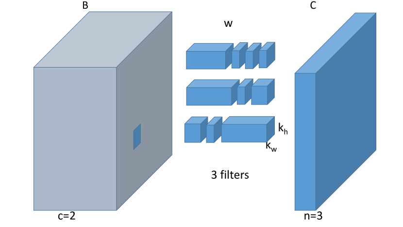
Figure 4: Filter-wise pruning for accelerating the first convolutional layer on the residual branch. We aim to reduce the number of channels filter-wise in weights $\mathrm{W}$, while minimizing the reconstruction error on feature map C. Channels of feature map B is not pruned. We apply our Eqn. 1 to each filter independently (each filter chooses its own representative input channels). $c,n$: number of channels for feature maps B and C, $k_{h}\times k_{w}$: kernel size.

Filter-wise pruning is another option for the first convolution on the residual branch, shown in Figure 4. Since the input channels of parameter-free shortcut branch could not be pruned, we apply our Eqn. 1 to each filter independently (each filter chooses its own representative input channels). It outputs ”irregular” convolutional layers, which need special library implementation support.

3.5 Combined with Tensor Factorization

Channel pruning can be easily combined method with tensor factorization, quantization, and lowbits etc. We focus on combination with tensor factorization.

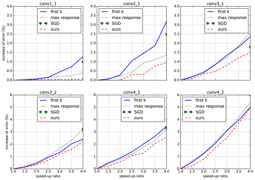
Figure 5: Single layer performance analysis under different speed-up ratios (without fine-tuning), measured by increase of error. To verify the importance of channel selection refered in Sec. 3.1, we considered three naive baselines. first k selects the first $k$ feature maps. max response selects channels based on absolute sum of corresponding weights filter [11]. SGD is a simple SGD alternative of our approach. Our approach is consistently better (smaller is better).

In general, tensor factorization could be represent as:

$$W^{l_{n}}=W_{1}\cdot W_{2}\cdot...\cdot W_{n}$$ (6)

Here, $W^{l_{n}}$ is the original convolutional layer filters for layer $n$, and $W_{1}\cdot W_{2}\cdot...\cdot W_{n}$ are several decomposed weights of the same size as $W$. Since the input and output channels of tensor factorization methods could not shrink, it becomes a bottleneck when reaching high ./We apply channels reduction on first and last weights decomposed layers, namely the output of $W_{n}$ and the input of $W_{1}$. In our experiments (Sec. 4.1.3), we combined [4], [14] and our approach. First, a $3\times 3$ weights is decomposed to $3\times 1,1\times 3,1\times 1$. Then our approach is applied to $3\times 1$ and $1\times 1$ weights.

3.6 Fine-tuning

We fine-tune the approximated model end-to-end on training data, which could gain more accuracy after reduction. We found that since the network is in a pretty unstable state, fine-tuning is very sensitive to the learning rate. The learning rate needs to be small enough. Otherwise, the accuracy quickly drops. If the learning rate is large, the finetuning process may jump out of the initialized local optimum by the pruned network and behave very similar to training the pruned architecture from scratch (Table V).

On ImageNet, we use learning rate of $1e^{-5}$ and a mini-batch size of 128. Fine-tune the models for ten epochs in the Imagenet training data (1/12 iterations of training from scratch). On CIFAR-10, we use learning rate of $1e^{-4}$ and a mini-batch size of 128 and fine-tune the models for 6000 iterations (training from scratch need 64000 iterations).

4 Experiment

TABLE I: The VGG-16 architecture. The column ”complexity” is portion of the theoretical time complexity each layer contributes. The column ”PCA energy” shows feature map PCA Energy (top 50% eigenvalues).

	# channels	# filters	output size	complexity (%)	PCA energy (%)
conv1_1	64	64	224	0.6	99.8
conv1_2	64	64	224	12	99.0
pool1			112
conv2_1	64	128	112	6	96.7
conv2_2	128	128	112	12	92.9
pool2			56
conv3_1	128	256	56	6	94.8
conv3_2	256	256	56	12	92.3
conv3_3	256	256	56	12	89.3
pool3			28
conv4_1	256	512	28	6	89.9
conv4_2	512	512	28	12	86.5
conv4_3	512	512	28	12	81.8
pool4			14
conv5_1	512	512	14	3	83.4
conv5_2	512	512	14	3	83.1
conv5_3	512	512	14	3	80.8

TABLE II: Accelerating the VGG-16 model [55] using a speedup ratio of $2\times$, $4\times$, or $5\times$ (smaller is better).

Increase of top-5 error (1-view, baseline 89.9%)
Solution	$2\times$	$4\times$	$5\times$
Jaderberg et al. [4] ([14]’s impl.)	-	9.7	29.7
Asym. [14]	0.28	3.84	-
Filter pruning [11] (fine-tuned, our impl.)	0.8	8.6	14.6
RNP [16]	-	3.23	3.58
SPP [17]	0.3	1.1	2.3
Ours (without fine-tune)	2.7	7.9	22.0
Ours (fine-tuned)	0	1.0	1.7

We evaluation our approach for the popular VGG Nets [55], ResNet [8], Xception [9] on ImageNet [56], CIFAR-10 [57] and PASCAL VOC 2007 [58].

For Batch Normalization [59], we first merge it into convolutional weights, which do not affect the outputs of the networks. So that each convolutional layer is followed by ReLU [60]. We use Caffe [61] for deep network evaluation, TensorFlow [62] for SGD implementation (Sec. 4.1.1) and scikit-learn [63] for solvers implementation. For channel pruning, we found that it is enough to extract 5000 images, and ten samples per image, which is also efficient (i.e., several minutes for VGG-16 , Sec. 4.1.2). On ImageNet, we evaluate the top-5 accuracy with the single view. Images are resized such that the shorter side is 256. The testing is on the center crop of $224\times 224$ pixels. The augmentation for fine-tuning is the random crop of $224\times 224$ and mirror.

4.1 Experiments with VGG-16

VGG-16 [55] is a 16 layers single-branch convolutional neural network, with 13 convolutional layers. It is widely used for recognition, detection and segmentation, etc. Single view top-5 accuracy for VGG-16 is 89.9%.

4.1.1 Single Layer Pruning

In this subsection, we evaluate single layer acceleration performance using our algorithm in Sec. 3.1. For better understanding, we compare our algorithm with there naive channel selection strategies. first k selects the first k channels. max response selects channels based on corresponding filters that have high absolute weights sum [11]. SGD is a simple alternative of our approach to use the original weights as initialization, as solve the $\ell_{1}$ regularized problem in Eqn. 2 (w.r.t. both the weights and connections) by stochastic gradient descent.

For fair comparison, we obtain the feature map indexes selected by each of them, then perform reconstruction (except SGD, Sec. 3.2.2). We hope that this could demonstrate the importance of channel selection. Performance is measured by the increase of error after a certain layer is pruned without fine-tuning, shown in Fig. 5.

As expected, error increases as  /increases. Our approach is consistently better than other approaches in different convolutional layers under different ./Unexpectedly, sometimes max response is even worse than first k. We argue that max response ignores correlations between different filters. Filters with large absolute weight may have a strong correlation. Thus selection based on filter weights is less meaningful. Correlation on feature maps is worth exploiting. We can find that channel selection affects reconstruction error a lot. Therefore, it is important for channel pruning.

As for SGD, we only performed experiments under $4\times$ speed-up due to time limitation. Though it shares same optimization goal with our approach, simple SGD seems difficult to optimize to an ideal local minimal. Shown in Figure 5, SGD is obviously worse than our optimization method.

Also notice that channel pruning gradually becomes hard, from shallower to deeper layers. It indicates that shallower layers have much more redundancy, which is consistent with [14]. We could prune more aggressively on shallower layers in whole model acceleration.

4.1.2 Whole Model Pruning

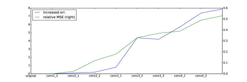
Figure 6: Accumulated layerwise pruning error for accelerating VGG-16 under $4\times$. ”relative MSE” is the relative mean square error. After fine-tuning, the Top-5 drops is 1.0%.

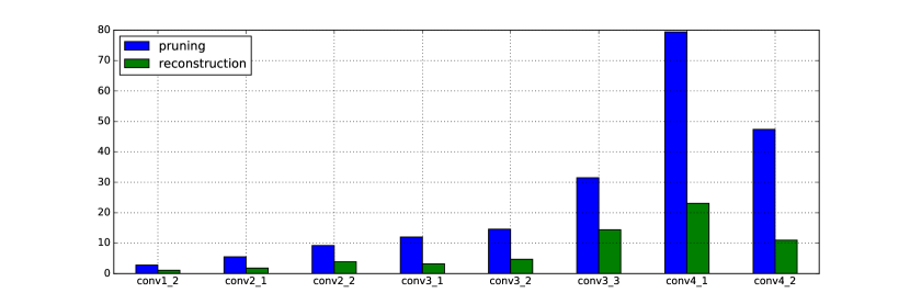
Figure 7: Time consumption for pruning VGG-16 under $4\times$, on Intel Xeon E5-2670 CPU (measured by seconds, time consumption may vary a little in each run). Our algorithm is very efficient.

Shown in Table I, we analyzed PCA energy of VGG-16. It indicates that shallower layers of VGG-16 are more redundant, which coincides with our single layer experiments above. So we prune more aggressive for shallower layers. Preserving channels ratios for shallow layers (conv1_x to conv3_x) and deep layers (conv4_x) is $1:1.5$. conv5_x are not pruned, since they only contribute 9% computation in total and are not redundant, shown in Table I.

We adopt the layer-by-layer whole model pruning proposed in Sec. 3.3. Figure 6 shows pruning VGG-16 under $4\times$ speed-up, which finally reach 1.0% increased of error after fine-tuning. It’s easy to see that accumulated error grows layer-by-layer. And errors are mainly introduced by pruning latter layers, which coincides with our observation from single layer pruning and PCA analysis.

Apart from the efficient inference model we attained, our algorithm is also efficient. Shown in Figure 7, our algorithm could finish pruning VGG-16 under $4\times$ within 5 minutes.

Shown in Table II, whole model acceleration results under $2\times$, $4\times$, $5\times$ are demonstrated. After fine-tuning, we could reach $2\times$ speed-up without losing accuracy. Under $4\times$, we only suffers 1.0% drops. Consistent with single layer analysis, our approach outperforms other recent pruning approaches (Filter Pruning [11], Runtime Neural Pruning [16] and Structured Probabilistic Pruning [17]) by a large margin. This is because we fully exploit channel redundancy within feature maps. Compared with tensor factorization algorithms, our approach is better than Jaderberg et al. [4], without fine-tuning. Though worse than Asym. [14], our combined model outperforms its combined Asym. 3D (Table III). This may indicate that channel pruning is more challenging than tensor factorization, since removing channels in one layer might dramatically change the input of the following layer. However, channel pruning keeps the original model architecture, do not introduce additional layers, and the absolute  /on GPU is much higher (Table VII).

4.1.3 Combined with Orthogonal Approaches

TABLE III: Performance of combined methods on the VGG-16 model [55] using a  /of $4\times$ or $5\times$. Our 3C solution outperforms previous approaches. The top-5 error rate (1-view) of the baseline VGG-16 model is 10.1%. (smaller is better).

Increase of top-5 error (1-view)
Solution	$4\times$	$5\times$
Asym. 3D [14]	0.9	2.0
Asym. 3D (fine-tuned) [14]	0.3	1.0
Our 3C	0.7	1.3
Our 3C (fine-tuned)	0.0	0.3

Since our approach exploits a new cardinality, we further combine our channel pruning with spatial factorization [4] and channel factorization [14] (Sec 3.5). Demonstrated in Table III, our 3 cardinalities acceleration (spatial, channel factorization, and channel pruning, denoted by 3C) outperforms previous state-of-the-arts. Asym. 3D [14] (spatial and channel factorization), factorizes a convolutional layer to three parts: $1\times 3,\ 3\times 1,\ 1\times 1$.

We apply spatial factorization, channel factorization, and our channel pruning together sequentially layer-by-layer. We fine-tune the accelerated models for 20 epochs, since they are three times deeper than the original ones. After fine-tuning, our $4\times$ model suffers no degradation. Clearly, a combination of different acceleration techniques is better than any single one. This indicates that a model is redundant in each cardinality.

4.1.4 Performance without Output Reconstruction

We evaluate whole model pruning performance without output reconstruction, to verify the effectiveness of the subproblem of $\mathrm{W}$ (Sec. 3.2.2). Shown in Table IV, without reconstruction, the accumulated error will be unacceptable for multi-layer pruning. Without reconstruction, the error increases to 99%. Even after fine-tuning the score is still much worse than the counterparts. This is because the LASSO step (Sec. 3.2.1) only updates $\boldsymbol{\beta}$ with limited freedom ($dimensionality=c$), thus it is insufficient for reconstruction. So we must adapt original weights $\mathrm{W}$ ($n\times c\times k_{h}\times k_{w}$) to the pruned input channels.

TABLE IV: Accelerating VGG-16 under $4\times$ with or without subproblem $\boldsymbol{\beta}$. It’s clear that without reconstruction the error increases. The top-5 error rate (1-view) of the baseline VGG-16 model is 10.1%.

Increase of top-5 err. (1-view)
approach	before fine-tuning	fine-tuned
Ours	7.9	1.0
Without subproblem $\boldsymbol{\beta}$	99	3.6

4.1.5 Comparisons with Training from Scratch

TABLE V: Comparisons with training from scratch, under $4\times$ acceleration on the VGG-16 model. Our fine-tuned model outperforms scratch trained counterparts. The top-5 error rate (1-view) of the baseline VGG-16 model is 10.1%. (smaller is better).

	Top-5 err.	Increased err.
From scratch	11.9	1.8
From scratch (uniformed)	12.5	2.4
Ours	18.0	7.9
Ours (fine-tuned)	11.1	1.0

Though training a compact model from scratch is time-consuming (usually 120 epochs), it worths comparing our approach and from scratch counterparts. To be fair, we evaluated both from scratch counterpart, and normal setting network that has the same computational complexity and same architecture.

Shown in Table V, we observed that it’s difficult for from scratch counterparts to reach competitive accuracy. Our model outperforms from scratch one. Our approach successfully picks out informative channels and constructs highly compact models. We can safely draw the conclusion that the same model is difficult to be obtained from scratch. This coincides with architecture design studies [64, 10] that the model could be easier to train if there are more channels in shallower layers. However, channel pruning favors shallower layers.

For from scratch (uniformed), the filters in each layer are reduced by half (e.g., reduce conv1_1 from 64 to 32). We can observe that normal setting networks of the same complexity couldn’t reach the same accuracy either. This consolidates our idea that there’s much redundancy in networks while training. However, redundancy can be opt-out at inference time. This may be an advantage of inference-time acceleration approaches over training-based approaches.

Notice that there’s a 0.6% gap between the from scratch model and the uniformed one, which indicates that there’s room for model exploration. Adopting our approach is much faster than training a model from scratch, even for a thinner one. Further researches could alleviate our approach to do thin model exploring.

4.1.6 Top-1 vs Top-5 Accuracy

TABLE VI: Increase of Top-1 and Top-5 error for accelerating VGG-16 on ImageNet. VGG-16 model’s Top-5 and Top-1 error baselines are 29.5% and 10.1% respectively.

Model	Top-1		Top-5
	err.	increased err.	err.	increased err.
$2\times$, fine-tuned	29.5	0.0	10.1	0.0
$4\times$, fine-tuned	31.7	2.2	11.1	1.0
$5\times$, fine-tuned	32.4	2.9	11.8	1.7
3C, $4\times$, fine-tuned	29.2	-0.3	10.1	0.0
3C, $5\times$, fine-tuned	29.5	0.0	10.4	0.3
From scratch	31.9	2.4	11.9	1.8
From scratch (uniformed)	32.9	3.4	12.5	2.4

Though our approach already achieved good performance with Top-5 accuracy, it is still possible that it can lead to significant Top-1 accuracy decrease. Shown in Table VI, we compare increase of Top-1 and Top-5 error for accelerating VGG-16 on ImageNet. Though the absolute drop is slightly larger, Top-1 is still consistent with top-5 results. For 3C $4\times$ and $5\times$, the Top-1 accuracy is even better. 3C $4\times$ Top-1 accuracy outperforms the original VGG-16 model by 0.3%.

4.1.7 Comparisons of Absolute Performance

TABLE VII: GPU acceleration comparison. We measure forward-pass time per image. Our approach generalizes well on GPU. The top-5 error rate (1-view) of the baseline VGG-16 model is 10.1%. (smaller is better).

Model	Solution	Increased err.	GPU time/ms
VGG-16	-	0	$8.144\,125$
VGG-16 ($4\times$)	Jaderberg et al. [4] ([14]’s impl.)	9.7	$8.050\,593\,75$ ($1.01\times$)
	Asym. [14]	3.8	$5.243\,625$ ($1.55\times$)
	Asym. 3D [14]	0.9	$8.503\,187\,5$ ($0.96\times$)
	Asym. 3D (fine-tuned) [14]	0.3	$8.503\,187\,5$ ($0.96\times$)
	Ours (fine-tuned)	1.0	3.264 ($2.50\times$)
	Our 3C (fine-tuned)	0.0	3.712 ($2.19\times$)

We further evaluate absolute performance of acceleration on GPU. Results in Table VII are obtained under Caffe [61], CUDA8 [65] and cuDNN5 [66], with a mini-batch of 32 on a GPU. Results are averaged from 50 runs. Tensor factorization approaches decompose weights into too many pieces, which heavily increase overhead. They could not gain much absolute speed-up. Though our approach also encountered performance decadence, it generalizes better on GPU than other approaches. Our results for tensor factorization differ from previous research [14, 4], maybe because current library and hardware prefer single large convolution instead of several small ones.

4.1.8 Acceleration for Detection

VGG-16 is popular among object detection tasks [67, 68, 69, 70, 71, 72, 73]. We evaluate transfer learning ability of our $2\times$/$4\times$ pruned VGG-16, for Faster R-CNN [74] object detections. PASCAL VOC 2007 object detection benchmark [58] contains 5k trainval images and 5k test images. The performance is evaluated by mean Average Precision (mAP) and mmAP (AP at IoU=.50:.05:.95, primary challenge metric of COCO [75]). In our experiments, we first perform channel pruning for VGG-16 on the ImageNet. Then we use the pruned model as the pre-trained model for Faster R-CNN.

TABLE VIII: $2\times$, $4\times$ acceleration for Faster R-CNN detection. mmAP is AP at IoU=.50:.05:.95 (primary challenge metric of COCO [75]).

	aero	bike	bird	boat	bottle	bus	car	cat	chair	cow	table	dog	horse	mbike	person	plant	sheep	sofa	train	tv	mAP	mmAP
orig	68.5	78.1	67.8	56.6	54.3	75.6	80.0	80.0	49.4	73.7	65.5	77.7	80.6	69.9	77.5	40.9	67.6	64.6	74.7	71.7	68.7	36.7
$2\times$	69.6	79.3	66.2	56.1	47.6	76.8	79.9	78.2	50.0	73.0	68.2	75.7	80.5	74.8	76.8	39.1	67.3	66.8	74.5	66.1	68.3	36.7
$4\times$	67.8	79.1	63.6	52.0	47.4	78.1	79.3	77.7	48.3	70.6	64.4	72.8	79.4	74.0	75.9	36.7	65.1	65.1	76.1	64.6	66.9	35.1

The actual running time of Faster R-CNN is 220ms / image. The convolutional layers contributes about 64%. We got actual time of 94ms for $4\times$ acceleration. From Table VIII, we observe 0.4% mAP and 0.0% mmAP drops of our $2\times$ model, which is not harmful for practice consideration. Observed from mmAP, For higher localization requirements our speedup model does not suffer from large degradation.

4.2 Experiments with Residual Architecture Nets

For Multi-path networks [7, 8, 9], we further explore the popular ResNet [8] and latest Xception [9], on ImageNet and CIFAR-10. Pruning residual architecture nets is more challenging. These networks are designed for both efficiency and high accuracy. Tensor factorization algorithms [14, 4] are not applicable to these model. Spatially, $1\times 1$ convolution is favored, which could hardly be factorized.

4.2.1 Filter-wise Pruning

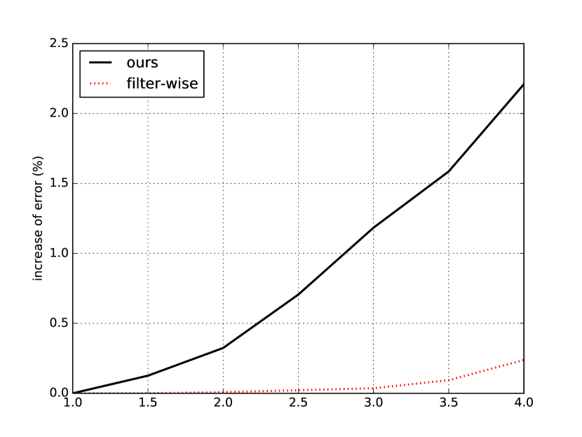
Figure 8: filter-wise pruning performance analysis under different speed-up ratios (without fine-tuning), measured by increase of error on VGG-16 conv3_2. (smaller is better).

Under single layer acceleration, filter-wise pruning (Sec. 3) is more accurate than our original one, since it is more flexible, shown in . From our ResNet pruning experiments in the next section, it improves 0.5% top-5 accuracy for $2\times$ ResNet-50 (applied on the first layer of each residual branch) without fine-tuning. However, after fine-tuning, there’s no noticeable improvement. Besides, it outputs ”irregular” convolutional layers, which need special library implementation support to gain practical speed-up. Thus, we did not adopt it for our residual architecture nets.

4.2.2 ResNet Pruning

TABLE IX: ResNet-50 Computational Complexity (bottleneck structure). ResNet-50 complexity uniformly drops on each residual block. $ix$ stands for the $x$th block of $i$th stage, $i=2,3,4,5,x=a,b,c$. The ”Complexity” column is the portion of computation complexity each block contributes.

layer name	Complexity (‰)
conv1	30
$2a_{1}$	13
$2a_{2a}$	3
$ia_{1}$	26
$ia_{2a}$	6
$ix_{2a}$	13
$ix_{2b}$	29
$ix_{2c}$	13

TABLE X: $2\times$ acceleration for ResNet-50 on ImageNet, the baseline network’s top-5 accuracy is 92.2% (one view). We improve performance with multi-branch enhancement (Sec. 3, smaller is better).

Solution	Speedup	Increased err.
ThiNet [15]	$1.58\times$	1.53
SPP [17]	$2\times$	1.8
Ours	2$\times$	8.0
Ours (enhanced)		4.0
Ours (enhanced, fine-tuned)		1.4

ResNet complexity uniformly drops on each residual block, as is shown in Table IX. Guided by single layer experiments (Sec. 4.1.1), we still prefer reducing shallower layers heavier than deeper ones.

Following similar setting as Filter pruning [11], we keep 70% channels for sensitive residual blocks (res5 and blocks close to the position where spatial size change, e.g. res3a,res3d). As for other blocks, we keep 30% channels. With the multi-branch enhancement, we prune branch2a more aggressively within each residual block. The preserving channels ratios for branch2a,branch2b,branch2c is $2:4:3$ (e.g., Given 30%, we keep 40%, 80%, 60% respectively).

We evaluate the performance of multi-branch variants of our approach (Sec. 3). Our approach outperforms recent approaches (ThiNet [15], Structured Probabilistic Pruning [17]) by a large margin. From Table X, we improve 4.0% with our multi-branch enhancement. This is because we accounted the accumulated error from shortcut connection which could broadcast to every layer after it. And the large input feature map width at the entry of each residual block is well reduced by our feature map sampling.

4.2.3 Xception Pruning

TABLE XI: Comparisons for Xception-50, under $2\times$ acceleration ratio. The baseline network’s top-5 accuracy is 92.8%. Our approach outperforms previous approaches. Most structured simplification methods are not effective on Xception architecture (smaller is better).

Solution	Increased err.
Filter pruning [11] (our impl.)	92.8
Filter pruning [11] (fine-tuned, our impl.)	4.3
Ours	2.9
Ours (fine-tuned)	1.0

Since computational complexity becomes important in model design, separable convolution has been payed much attention [76, 9]. Xception [9] is already spatially optimized and tensor factorization on $1\times 1$ convolutional layer is destructive. Thanks to our approach, it could still be accelerated with graceful degradation. For the ease of comparison, we adopt Xception convolution on ResNet-50, denoted by Xception-50. Based on ResNet-50, we swap all convolutional layers with spatial conv blocks. To keep the same computational complexity, we increase the input channels of all branch2b layers by $2\times$. The baseline Xception-50 has a top-5 accuracy of 92.8% and complexity of 4450 MFLOPs.

We apply multi-branch variants of our approach as described in Sec. 3, and adopt the same pruning ratio setting as ResNet in the previous section. Maybe because of Xception block is unstable, Batch Normalization layers must be maintained during pruning. Otherwise, it becomes non-trivial to fine-tune the pruned model.

Shown in Table XI, after fine-tuning, we only suffer 1.0% increase of error under $2\times$. Filter pruning [11] could also apply on Xception, though it is designed for small ./Without fine-tuning, the top-5 error is 100%. After training 20 epochs, the increased error reach 4.3% which is like training from scratch. Our results for Xception-50 are not as graceful as results for VGG-16 since modern networks tend to have less redundancy by design.

4.2.4 Experiments on CIFAR-10

Even though our approach is designed for large datasets, it could generalize well on small datasets. We perform experiments on CIFAR-10 dataset [57], which is favored by many acceleration studies. It consists of 50k images for training and 10k for testing in 10 classes. The original $32\times 32$ image is zero padded with 4 pixels on each side, then random cropped to $32\times 32$ at training time. Our approach could be finished within minutes.

TABLE XII: $1.4\times$ and $2\times$ speed-up comparisons for ResNet-56 on CIFAR-10, the baseline accuracy is 92.8% (one view). We outperforms previous approaches and scratch trained counterpart (smaller is better).

Model	$1.4\times$		$2\times$
	err.	increased err.	err.	increased err.
Filter pruning [11] (fine-tuned, our impl.)	7.2	0.0	8.5	1.3
From scratch	7.8	0.6	9.1	1.9
Ours	7.7	0.5	9.2	2.0
Ours (fine-tuned)	7.2	0.0	8.2	1.0
from scratch (uniformed)	-		8.7	1.5
ours (uniformed)			10.2	3.0
ours (uniformed, fine-tuned)			8.6	1.4

We reproduce ResNet-56, which has accuracy of 92.8% (Serve as a reference, the official ResNet-56 [8] has accuracy of 93.0%). For $2\times$ acceleration, we follow similar setting as Sec. 4.2.2 (keep the final stage unchanged, where the spatial size is $8\times 8$). Shown in Table XII, our approach is competitive with scratch trained one, without fine-tuning, under both $1.4\times$ and $2\times$ speed-up. After fine-tuning, our result is significantly better than Filter pruning [11] and scratch trained one for both $1.4\times$ and $2\times$ acceleration.

Reduce Shallow vs. Deep layers: Denoted by (uniform) in Table XII, uniformed solution prune each layer while the same pruning ratio. Clearly, our uniformed results are worse than shallow layers heavily reduced ones. However, uniformed model from scratched is better than its counterpart. This is because channel pruning favors less channels on shallow layers, however from scratch models performs better with more shallower layers. It indicates that redundancy on shallow layers is necessary while training, which could be removed at inference time.

5 Conclusion

To conclude, current deep CNNs are accurate with high inference costs. In this paper, we have presented an inference-time channel pruning method for very deep networks. The reduced CNNs are inference efficient networks while maintaining accuracy, and only require off-the-shelf libraries. Compelling speed-ups and accuracy are demonstrated for both VGG Net and ResNet-like networks on ImageNet, CIFAR-10 and PASCAL VOC 2007.

In the future, we plan to involve our approaches to training time to accelerate training procedure, instead of inference time only.

References

- [1] C. Szegedy, V. Vanhoucke, S. Ioffe, J. Shlens, and Z. Wojna, “Rethinking the inception architecture for computer vision,” arXiv preprint arXiv:1512.00567, 2015.
- [2] N. Vasilache, J. Johnson, M. Mathieu, S. Chintala, S. Piantino, and Y. LeCun, “Fast convolutional nets with fbfft: A gpu performance evaluation,” arXiv preprint arXiv:1412.7580, 2014.
- [3] M. Courbariaux and Y. Bengio, “Binarynet: Training deep neural networks with weights and activations constrained to+ 1 or-1,” arXiv preprint arXiv:1602.02830, 2016.
- [4] M. Jaderberg, A. Vedaldi, and A. Zisserman, “Speeding up convolutional neural networks with low rank expansions,” arXiv preprint arXiv:1405.3866, 2014.
- [5] S. Han, J. Pool, J. Tran, and W. Dally, “Learning both weights and connections for efficient neural network,” in Advances in Neural Information Processing Systems, 2015, pp. 1135–1143.
- [6] W. Wen, C. Wu, Y. Wang, Y. Chen, and H. Li, “Learning structured sparsity in deep neural networks,” in Advances In Neural Information Processing Systems, 2016, pp. 2074–2082.
- [7] C. Szegedy, W. Liu, Y. Jia, P. Sermanet, S. Reed, D. Anguelov, D. Erhan, V. Vanhoucke, and A. Rabinovich, “Going deeper with convolutions,” in Proceedings of the IEEE Conference on Computer Vision and Pattern Recognition, 2015, pp. 1–9.
- [8] K. He, X. Zhang, S. Ren, and J. Sun, “Deep residual learning for image recognition,” in Proceedings of the IEEE conference on computer vision and pattern recognition, 2016, pp. 770–778.
- [9] F. Chollet, “Xception: Deep learning with depthwise separable convolutions,” arXiv preprint arXiv:1610.02357, 2016.
- [10] J. M. Alvarez and M. Salzmann, “Learning the number of neurons in deep networks,” in Advances in Neural Information Processing Systems, 2016, pp. 2262–2270.
- [11] H. Li, A. Kadav, I. Durdanovic, H. Samet, and H. P. Graf, “Pruning filters for efficient convnets,” arXiv preprint arXiv:1608.08710, 2016.
- [12] S. Anwar and W. Sung, “Compact deep convolutional neural networks with coarse pruning,” arXiv preprint arXiv:1610.09639, 2016.
- [13] T. Chen, I. Goodfellow, and J. Shlens, “Net2net: Accelerating learning via knowledge transfer,” arXiv preprint arXiv:1511.05641, 2015.
- [14] X. Zhang, J. Zou, K. He, and J. Sun, “Accelerating very deep convolutional networks for classification and detection,” IEEE transactions on pattern analysis and machine intelligence, vol. 38, no. 10, pp. 1943–1955, 2016.
- [15] J.-H. Luo, J. Wu, and W. Lin, “Thinet: A filter level pruning method for deep neural network compression,” in Proceedings of the IEEE Conference on Computer Vision and Pattern Recognition, 2017, pp. 5058–5066.
- [16] J. Lin, Y. Rao, and J. Lu, “Runtime neural pruning,” in Advances in Neural Information Processing Systems, 2017, pp. 2178–2188.
- [17] H. Wang, Q. Zhang, Y. Wang, and R. Hu, “Structured probabilistic pruning for deep convolutional neural network acceleration,” arXiv preprint arXiv:1709.06994, 2017.
- [18] Z. Liu, J. Li, Z. Shen, G. Huang, S. Yan, and C. Zhang, “Learning efficient convolutional networks through network slimming,” in Proceedings of the IEEE Conference on Computer Vision and Pattern Recognition, 2017, pp. 2736–2744.
- [19] Y. He, X. Zhang, and J. Sun, “Channel pruning for accelerating very deep neural networks,” in The IEEE International Conference on Computer Vision (ICCV), Oct 2017, pp. 1389–1397.
- [20] Y. Cheng, D. Wang, P. Zhou, and T. Zhang, “A survey of model compression and acceleration for deep neural networks,” arXiv preprint arXiv:1710.09282, 2017.
- [21] Y. LeCun, J. S. Denker, S. A. Solla, R. E. Howard, and L. D. Jackel, “Optimal brain damage.” in NIPs, vol. 2, 1989, pp. 598–605.
- [22] B. Hassibi and D. G. Stork, Second order derivatives for network pruning: Optimal brain surgeon. Morgan Kaufmann, 1993.
- [23] H. Bagherinezhad, M. Rastegari, and A. Farhadi, “Lcnn: Lookup-based convolutional neural network,” arXiv preprint arXiv:1611.06473, 2016.
- [24] M. Rastegari, V. Ordonez, J. Redmon, and A. Farhadi, “Xnor-net: Imagenet classification using binary convolutional neural networks,” in European Conference on Computer Vision. Springer, 2016, pp. 525–542.
- [25] M. Mathieu, M. Henaff, and Y. LeCun, “Fast training of convolutional networks through ffts,” arXiv preprint arXiv:1312.5851, 2013.
- [26] A. Lavin, “Fast algorithms for convolutional neural networks,” arXiv preprint arXiv:1509.09308, 2015.
- [27] H. Phan, Y. He, M. Savvides, Z. Shen et al., “Mobinet: A mobile binary network for image classification,” in Proceedings of the IEEE/CVF Winter Conference on Applications of Computer Vision, 2020, pp. 3453–3462.
- [28] B. Liu, M. Wang, H. Foroosh, M. Tappen, and M. Pensky, “Sparse convolutional neural networks,” in Proceedings of the IEEE Conference on Computer Vision and Pattern Recognition, 2015, pp. 806–814.
- [29] V. Lebedev and V. Lempitsky, “Fast convnets using group-wise brain damage,” arXiv preprint arXiv:1506.02515, 2015.
- [30] S. Han, X. Liu, H. Mao, J. Pu, A. Pedram, M. A. Horowitz, and W. J. Dally, “Eie: efficient inference engine on compressed deep neural network,” in Proceedings of the 43rd International Symposium on Computer Architecture. IEEE Press, 2016, pp. 243–254.
- [31] Y. Guo, A. Yao, and Y. Chen, “Dynamic network surgery for efficient dnns,” in Advances In Neural Information Processing Systems, 2016, pp. 1379–1387.
- [32] H. Zhong, X. Liu, Y. He, and Y. Ma, “Shift-based primitives for efficient convolutional neural networks,” arXiv preprint arXiv:1809.08458, 2018.
- [33] Y. He, X. Liu, H. Zhong, and Y. Ma, “Addressnet: Shift-based primitives for efficient convolutional neural networks,” in 2019 IEEE Winter conference on applications of computer vision (WACV). IEEE, 2019, pp. 1213–1222.
- [34] T.-J. Yang, Y.-H. Chen, and V. Sze, “Designing energy-efficient convolutional neural networks using energy-aware pruning,” arXiv preprint arXiv:1611.05128, 2016.
- [35] S. Han, H. Mao, and W. J. Dally, “Deep compression: Compressing deep neural network with pruning, trained quantization and huffman coding,” CoRR, abs/1510.00149, vol. 2, 2015.
- [36] V. Lebedev, Y. Ganin, M. Rakhuba, I. Oseledets, and V. Lempitsky, “Speeding-up convolutional neural networks using fine-tuned cp-decomposition,” arXiv preprint arXiv:1412.6553, 2014.
- [37] Y. Gong, L. Liu, M. Yang, and L. Bourdev, “Compressing deep convolutional networks using vector quantization,” arXiv preprint arXiv:1412.6115, 2014.
- [38] Y.-D. Kim, E. Park, S. Yoo, T. Choi, L. Yang, and D. Shin, “Compression of deep convolutional neural networks for fast and low power mobile applications,” arXiv preprint arXiv:1511.06530, 2015.
- [39] Y. He, J. Qian, and J. Wang, “Depth-wise decomposition for accelerating separable convolutions in efficient convolutional neural networks,” in Proceedings of the IEEE Conference on Computer Vision and Pattern Recognition Workshops, 2019.
- [40] J. Xue, J. Li, and Y. Gong, “Restructuring of deep neural network acoustic models with singular value decomposition.” in INTERSPEECH, 2013, pp. 2365–2369.
- [41] E. L. Denton, W. Zaremba, J. Bruna, Y. LeCun, and R. Fergus, “Exploiting linear structure within convolutional networks for efficient evaluation,” in Advances in Neural Information Processing Systems, 2014, pp. 1269–1277.
- [42] R. Girshick, “Fast r-cnn,” in Proceedings of the IEEE International Conference on Computer Vision, 2015, pp. 1440–1448.
- [43] X. Zhang and H. Yihui, “Image processing method and apparatus, and computer-readable storage medium,” Jul. 14 2020, uS Patent 10,713,533.
- [44] H. Zhou, J. M. Alvarez, and F. Porikli, “Less is more: Towards compact cnns,” in European Conference on Computer Vision. Springer International Publishing, 2016, pp. 662–677.
- [45] Y. LeCun, L. Bottou, Y. Bengio, and P. Haffner, “Gradient-based learning applied to document recognition,” Proceedings of the IEEE, vol. 86, no. 11, pp. 2278–2324, 1998.
- [46] A. Krizhevsky, I. Sutskever, and G. E. Hinton, “Imagenet classification with deep convolutional neural networks,” in Advances in neural information processing systems, 2012, pp. 1097–1105.
- [47] S. Anwar, K. Hwang, and W. Sung, “Structured pruning of deep convolutional neural networks,” arXiv preprint arXiv:1512.08571, 2015.
- [48] A. Polyak and L. Wolf, “Channel-level acceleration of deep face representations,” IEEE Access, vol. 3, pp. 2163–2175, 2015.
- [49] Y. He, J. Lin, Z. Liu, H. Wang, L.-J. Li, and S. Han, “Amc: Automl for model compression and acceleration on mobile devices,” in European Conference on Computer Vision, Sept 2018.
- [50] S. Srinivas and R. V. Babu, “Data-free parameter pruning for deep neural networks,” arXiv preprint arXiv:1507.06149, 2015.
- [51] Z. Mariet and S. Sra, “Diversity networks,” arXiv preprint arXiv:1511.05077, 2015.
- [52] H. Hu, R. Peng, Y.-W. Tai, and C.-K. Tang, “Network trimming: A data-driven neuron pruning approach towards efficient deep architectures,” arXiv preprint arXiv:1607.03250, 2016.
- [53] R. Tibshirani, “Regression shrinkage and selection via the lasso,” Journal of the Royal Statistical Society. Series B (Methodological), pp. 267–288, 1996.
- [54] L. Breiman, “Better subset regression using the nonnegative garrote,” Technometrics, vol. 37, no. 4, pp. 373–384, 1995.
- [55] K. Simonyan and A. Zisserman, “Very deep convolutional networks for large-scale image recognition,” arXiv preprint arXiv:1409.1556, 2014.
- [56] J. Deng, W. Dong, R. Socher, L.-J. Li, K. Li, and L. Fei-Fei, “Imagenet: A large-scale hierarchical image database,” in Computer Vision and Pattern Recognition, 2009. CVPR 2009. IEEE Conference on. IEEE, 2009, pp. 248–255.
- [57] A. Krizhevsky and G. Hinton, “Learning multiple layers of features from tiny images,” 2009.
- [58] M. Everingham, L. Van Gool, C. K. I. Williams, J. Winn, and A. Zisserman, “The PASCAL Visual Object Classes Challenge 2007 (VOC2007) Results,” http://www.pascal-network.org/challenges/VOC/voc2007/workshop/index.html.
- [59] S. Ioffe and C. Szegedy, “Batch normalization: Accelerating deep network training by reducing internal covariate shift,” arXiv preprint arXiv:1502.03167, 2015.
- [60] V. Nair and G. E. Hinton, “Rectified linear units improve restricted boltzmann machines,” in Proceedings of the 27th international conference on machine learning (ICML-10), 2010, pp. 807–814.
- [61] Y. Jia, E. Shelhamer, J. Donahue, S. Karayev, J. Long, R. Girshick, S. Guadarrama, and T. Darrell, “Caffe: Convolutional architecture for fast feature embedding,” arXiv preprint arXiv:1408.5093, 2014.
- [62] M. Abadi, A. Agarwal, P. Barham, E. Brevdo, Z. Chen, C. Citro, G. S. Corrado, A. Davis, J. Dean, M. Devin, S. Ghemawat, I. Goodfellow, A. Harp, G. Irving, M. Isard, Y. Jia, R. Jozefowicz, L. Kaiser, M. Kudlur, J. Levenberg, D. Mané, R. Monga, S. Moore, D. Murray, C. Olah, M. Schuster, J. Shlens, B. Steiner, I. Sutskever, K. Talwar, P. Tucker, V. Vanhoucke, V. Vasudevan, F. Viégas, O. Vinyals, P. Warden, M. Wattenberg, M. Wicke, Y. Yu, and X. Zheng, “TensorFlow: Large-scale machine learning on heterogeneous systems,” 2015, software available from tensorflow.org. [Online]. Available: http://tensorflow.org/
- [63] F. Pedregosa, G. Varoquaux, A. Gramfort, V. Michel, B. Thirion, O. Grisel, M. Blondel, P. Prettenhofer, R. Weiss, V. Dubourg, J. Vanderplas, A. Passos, D. Cournapeau, M. Brucher, M. Perrot, and E. Duchesnay, “Scikit-learn: Machine learning in Python,” Journal of Machine Learning Research, vol. 12, pp. 2825–2830, 2011.
- [64] J. Huang, V. Rathod, C. Sun, M. Zhu, A. Korattikara, A. Fathi, I. Fischer, Z. Wojna, Y. Song, S. Guadarrama et al., “Speed/accuracy trade-offs for modern convolutional object detectors,” arXiv preprint arXiv:1611.10012, 2016.
- [65] J. Nickolls, I. Buck, M. Garland, and K. Skadron, “Scalable parallel programming with CUDA,” ACM Queue, vol. 6, no. 2, pp. 40–53, 2008. [Online]. Available: http://doi.acm.org/10.1145/1365490.1365500
- [66] S. Chetlur, C. Woolley, P. Vandermersch, J. Cohen, J. Tran, B. Catanzaro, and E. Shelhamer, “cudnn: Efficient primitives for deep learning,” CoRR, vol. abs/1410.0759, 2014. [Online]. Available: http://arxiv.org/abs/1410.0759
- [67] J. Redmon, S. K. Divvala, R. B. Girshick, and A. Farhadi, “You only look once: Unified, real-time object detection,” CoRR, vol. abs/1506.02640, 2015. [Online]. Available: http://arxiv.org/abs/1506.02640
- [68] W. Liu, D. Anguelov, D. Erhan, C. Szegedy, S. E. Reed, C. Fu, and A. C. Berg, “SSD: single shot multibox detector,” CoRR, vol. abs/1512.02325, 2015. [Online]. Available: http://arxiv.org/abs/1512.02325
- [69] C. Zhu, Y. He, and M. Savvides, “Feature selective anchor-free module for single-shot object detection,” in Proceedings of the IEEE/CVF conference on computer vision and pattern recognition, 2019, pp. 840–849.
- [70] Y. He and J. Wang, “Deep mixture density network for probabilistic object detection,” in 2020 IEEE/RSJ International Conference on Intelligent Robots and Systems (IROS). IEEE, 2020, pp. 10 550–10 555.
- [71] Y. He, C. Zhu, J. Wang, M. Savvides, and X. Zhang, “Bounding box regression with uncertainty for accurate object detection,” in Proceedings of the ieee/cvf conference on computer vision and pattern recognition, 2019, pp. 2888–2897.
- [72] Y. He and J. Wang, “Deep multivariate mixture of gaussians for object detection under occlusion,” 2019.
- [73] Y. He, X. Zhang, M. Savvides, and K. Kitani, “Softer-nms: Rethinking bounding box regression for accurate object detection,” arXiv preprint arXiv:1809.08545, vol. 2, no. 3, pp. 69–80, 2018.
- [74] S. Ren, K. He, R. B. Girshick, and J. Sun, “Faster R-CNN: towards real-time object detection with region proposal networks,” CoRR, vol. abs/1506.01497, 2015. [Online]. Available: http://arxiv.org/abs/1506.01497
- [75] T.-Y. Lin, M. Maire, S. Belongie, J. Hays, P. Perona, D. Ramanan, P. Dollár, and C. L. Zitnick, “Microsoft coco: Common objects in context,” in European conference on computer vision. Springer, Cham, 2014, pp. 740–755.
- [76] S. Xie, R. Girshick, P. Dollár, Z. Tu, and K. He, “Aggregated residual transformations for deep neural networks,” arXiv preprint arXiv:1611.05431, 2016.