Quantum simulation of dynamical phase transitions in noisy quantum devices

Abstract

Zero-noise extrapolation provides an especially useful error mitigation method for noisy intermediate-scale quantum devices. Our analysis, based on matrix product density operators, of the transverse-field Ising model with depolarizing noise, reveals both advantages and inherent problems associated with zero-noise extrapolation when simulating non-equilibrium many-body dynamics. On the one hand, interestingly, noise alters systematically the behavior of the Loschmidt echo at the dynamical phase transition times, doubling the number of non-analytic points, and hence inducing an error that, inherently, cannot be mitigated. On the other, zero-noise extrapolation may be employed to recover quantum revivals of the Loschmidt echo, which would be completely missed in the absence of mitigation, and to retrieve faithfully noise-free inter-site correlations. Our results, which are in good agreement with those obtained using quantum simulators, reveal the potential of matrix product density operators for the investigation of the performance of quantum devices with a large number of qubits and deep noisy quantum circuits.

Quantum computers may outperform their classical counterparts by exploiting the dimensionality of Hilbert space, which increases exponentially with the system size Nielsen and Chuang (2010); Feynman (1982); Lidar. and Brun (2013); Lloyd (1996). They enable a large number of possible applications, including quantum simulation, optimization, machine learning, and more Biamonte et al. (2017); Kandala et al. (2017); Nielsen and Chuang (2010). Despite major technical challenges, recent years have witnessed a rapid experimental progress on quantum computing using various platforms, including superconducting qubits Wendin (2017), trapped ion technologies Bruzewicz et al. (2019); Cirac and Zoller (1995); Blatt and Roos (2012), neutral atoms Jaksch et al. (1998); Bloch et al. (2012), semiconductor spin qubits Burkard et al. (2021), and photonics Slussarenko and Pryde (2019); Weedbrook et al. (2012).

Currently available quantum information processing devices are severely limited by noise and decoherence. For this reason, they are referred to as noisy intermediate-scale quantum (NISQ) devices Preskill (2018). These devices are limited to shallow quantum circuits, but, even then, noise can lead to faulty estimates. Although quantum error correction can, in principle, reduce or eliminate the effect of decoherence it is not possible to implement such schemes on present NISQ devices due to the complex entanglement resource required.

In response to the challenge of quantum noise, quantum error mitigation techniques have been developed for NISQ devices Temme et al. (2017); Endo et al. (2018); Li and Benjamin (2017) to ameliorate the deleterious effects of decoherence in a near-term compatible way. The two major general-purpose error mitigation methods are probabilistic error cancellation van den Berg et al. (2022) and zero-noise extrapolation (ZNE) Li and Benjamin (2017); Mari et al. (2021); Lowe et al. (2021). Although there have been several studies on the general performance of mitigation techniques Takagi et al. (2022a); Tsubouchi et al. (2022); Takagi et al. (2022b), the behavior of ZNE for large-scale quantum simulations is not well explored.

In this paper, we investigate, by means of matrix product density operators (MPDO) Verstraete et al. (2004); Zwolak and Vidal (2004); Cheng et al. (2021); Werner et al. (2016); Schollwöck (2011), the use of ZNE for the study of out-of-equilibrium quantum many-body systems. In particular, we evaluate the simulation of the dynamics of the transverse-field Ising model by means of a NISQ device with depolarizing noise, characterized by a noise channel $\mathcal{E}(\rho)=(1-p)\rho+p\frac{I}{2^{N}}$ Nielsen and Chuang (2010); Lidar. and Brun (2013), with $\rho$ the density matrix, $p$ the probabilistic error rate that depends on the device and the circuit, and $N$ the number of qubits. Although there are other possible noise channels, the depolarizing noise model often appropriately describes the average noise for large circuits involving many qubits and gates Urbanek et al. (2021). Our results indicate that, below a given noise and evolution-time threshold, ZNE may faithfully recover quantum revivals of the Loschmidt echo, which would be otherwise basically lost, as well as the inter-site correlation dynamics. However, we show that the noise-free dynamics during the time windows associated to dynamical quantum phase transitions (DQPTs) is inherently irretrievable using ZNE, due to the systematic noise-induced doubling of non-analytic points in the return rate. Our results, which are in good agreement with direct quantum simulations, show the potential of MPDO calculations for the study of NISQ devices with many qubits and deep circuits.

Model.–

We consider in the following the transverse-field Ising model  (TFIM):

$$\mathcal{H}=-\frac{1}{2}\left[\sum^{N-1}_{i=1}\left(J_{z}\sigma_{i}^{z}\sigma_{i+1}^{z}+J_{x}\sigma_{i}^{x}\sigma_{i+1}^{x}\right)+\sum^{N}_{i=1}h_{x}\sigma_{i}^{x}\right],$$ (1)

where $\sigma_{i}^{x,y,z}$ are the spin-$\frac{1}{2}$ Pauli matrices at the different lattice sites $i=1,\dots,N$, $h_{x}$ is the transverse field, and $J_{z}$ ($J_{x}$) denotes the $z$ ($x$) spin-spin coupling. For convenience, we assume open-boundary conditions. For $J_{x}=0$, the model reduces to the integrable transverse-field Ising chain, which is exactly solvable by a Jordan-Wigner mapping into non-interacting fermions Pfeuty (1970); Osborne and Nielsen (2002). To make the model generic, we add a weak $J_{x}$ term, which becomes equivalent to a two-particle interaction in the fermionic language, rendering the model non-integrable. In this work, we consider $J_{z}=J$, $J_{x}=0.1J$, and $h_{x}=0.1J$.

We are particularly interested in the non-equilibrium dynamics of Model (1) after a quench. Starting with a state $|\psi_{0}\rangle$, the Loschmidt echo is defined as the probability $\Lambda(t)=|\langle\psi_{0}|e^{-i{\cal H}t}|\psi_{0}\rangle|^{2}$ to find the time-evolved system in the initial state. The return-rate function, $\lambda(t)=-\lim\limits_{N\to\infty}\frac{1}{N}\log\Lambda(t)$, is the real-time analogous of the free-energy per site. Non-analiticities of $\lambda(t)$ at critical times indicate the presence of DQPTs Heyl et al. (2013); Heyl (2014, 2018, 2015); Karrasch and Schuricht (2013); Dborin et al. (2022); Halimeh and Zauner-Stauber (2017); Homrighausen et al. (2017); Lang et al. (2018); Van Damme et al. (2022a, b), which have been recently realized experimentally Jurcevic et al. (2017); Wu et al. (2022).

Master equation.–

In the presence of dissipation, the evolution of the density matrix $\rho$ of the system is given by the master equation Lidar. and Brun (2013); Nielsen and Chuang (2010),

$$\partial_{t}\rho= \mathcal{L}(t)[\rho]=-i[\mathcal{H},\rho(t)]$$

$$+\sum_{\begin{subarray}{c}i\\ \mu=x,y,z\end{subarray}}{\gamma_{i}\left(\sigma^{\mu}_{i}(t)\rho\sigma^{\mu\dagger}_{i}(t)-\frac{1}{2}\{\sigma^{\mu\dagger}_{i}(t)\sigma^{\mu}_{i}(t),\rho\}\right)}$$ (2)

where the first line provides the unitary part of the time evolution, whereas the second accounts for dissipation. The Lindblad (jump) operators for depolarizing noise are given by the Pauli operators $\sigma_{i}^{x,y,z}$, and encode the system-reservoir couplings, $\gamma_{i}$ characterizes the dissipation strength at site $i$, and $[]$ and $\{\}$ denote commutator and anti-commutator, respectively. For a time step $\delta t$, the probabilistic error is related to the noise strength through $p_{\delta t}=1-e^{-4\gamma\delta t}$ (see the Supplemental Material). Assuming a constant $\gamma$ for each jump operator, we may re-write Eq. (2) in the form:

$$\partial_{t}\rho_{\gamma}(t)={\cal L}[\rho_{\gamma}]=-i[\mathcal{H}(t),\rho_{\gamma}(t)]+\gamma\mathcal{D}(\rho_{\gamma}(t))$$ (3)

Zero-noise extrapolation.–

ZNE is a relatively simple error-mitigation technique, easy to implement in post-processing, and which requires neither knowledge of the noise, nor a gate-level control of the device. The method assumes the ability to scale the noise parameter to particular values $\alpha\gamma$ with $\alpha>1$. Assuming a constant noise rate, this may be achieved by a proper stretching of the time evolution by the factor $\alpha$, while reducing ${\cal H}\to{\cal H}/\alpha$, resulting in the same overall Hamiltonian evolution, whereas the noise increases to $\alpha\gamma$. This may be realized in practice by changing the duration and strength of the pulses that implement the desired operations. Alternatively one may employ unitary folding, where operations are added that do not affect the Hamiltonian evolution but increase the noise, e.g. for a unitary gate $\mathcal{u}$ one may use $\mathcal{U}\rightarrow\mathcal{U}\mathcal{U}\mathcal{U}^{\dagger}$ Temme et al. (2017); Kandala et al. (2019); Endo et al. (2021); Giurgica-Tiron et al. (2020); LaRose et al. (2022)(see the Supplemental Materia).

For extrapolation to zero noise value, $\gamma=0$, we employ the Richardson extrapolation technique Burden and Faires (2010); Giurgica-Tiron et al. (2020). Given a sequence of noise parameters $\alpha_{i}\gamma$ with $1=\alpha_{0}<\alpha_{1}<...<\alpha_{n}$, the estimated noiseless expectation value for an operator $M$ is $\langle M_{E}\rangle(\gamma=0)=\sum_{k=0}^{n}\beta_{k}\langle M\rangle(\alpha_{k}\gamma)$. The coefficients $\beta_{k}$ satisfy the relations $\sum^{n}_{k=0}\beta_{k}=1$ and $\sum^{n}_{l=0}\beta_{l}\alpha_{l}^{k}=0$, giving $\beta_{k}=\prod_{i\neq k}\frac{\alpha_{i}}{\alpha_{i}-\alpha_{k}}$ Endo et al. (2021); Temme et al. (2017); Kandala et al. (2019).

Matrix Product Density Operators.–

We use MPDOs to simulate noisy quantum circuits. MPDOs are an extension of matrix product states for simulating thermal or dissipative systems Verstraete et al. (2004); Zwolak and Vidal (2004); Schollwöck (2011). We employ an approach based on the work of Zwolak and Vidal Zwolak and Vidal (2004). Based on Choi’s isomorphism $\left|\psi\right\rangle\left\langle\phi\right|=\left|\psi\right\rangle\left|\phi\right\rangle=|{\psi\otimes\phi}\rrangle$, one can vectorize the density matrix $\rho=\left|\psi\right\rangle\left\langle\psi\right|\rightarrow|{\rho}\rrangle=|{\psi\otimes\psi}\rrangle$. Similar to the matrix-product states representation for a quantum state Montangero (2018); Javanmard et al. (2018); Schollwöck (2011); Cirac et al. (2021) $\left|\psi\right\rangle=\sum_{\{\sigma\}}{T^{\sigma_{1}}_{1}\ldots T^{\sigma_{N}}_{N}\left|\sigma_{1}\ldots\sigma_{N}\right\rangle}$, we have in the MPDO representation $|{\rho}\rrangle=\sum_{\{\sigma\sigma^{\prime}\}}{M^{\sigma_{1}\sigma^{\prime}_{1}}_{1}\ldots M^{\sigma_{N}\sigma^{\prime}_{N}}_{N}\left|\sigma_{1}\ldots\sigma_{N}\right\rangle\left\langle\sigma^{\prime}_{1}\ldots\sigma^{\prime}_{N}\right|}$, with $\sigma_{j}$ possible single-site states, and $M^{\sigma_{i},\sigma^{\prime}_{i}}_{i}=T^{\sigma_{i}}_{i}\otimes(T^{\sigma^{\prime}_{i}}_{i})^{\star}$. By reformulating the Liouvillian in a vectorized form $\mathcal{L}_{\#}$, and for a time-independent $\mathcal{L}_{\#}$, the time evolution is given by $|{\rho(T)}\rrangle=e^{T\mathcal{L}_{\#}}|{\rho(0)}\rrangle$. Here we consider the case where $\mathcal{L}_{\#}$ is a sum of nearest-neighbor interaction terms $\mathcal{L}_{\#}[\rho]=\sum_{\langle i,j\rangle}\mathcal{L}^{[i,j]}_{\#}[\rho]$. This structure allows for using time-evolving block decimation to simulate the time evolution (see the Supplemental Material).

In this work, we consider a chain with $N=32$ spins initially prepared in the state $\left|\psi_{0}\right\rangle=\left|+\right\rangle^{\bigotimes N}$, with $|+\rangle=H|\downarrow\rangle=\left(|\downarrow\rangle+|\uparrow\rangle\right)/\sqrt{2}$, with $\{|\uparrow\rangle,|\downarrow\rangle\}$ the eigenstates of $\sigma^{z}$, and $H$ the Hadamard gate. We evolve this state using Hamiltonian  (1). In our MPDO simulation, we use second-order Suzuki-Trotter decomposition Schollwöck (2011); Hatano and Suzuki (2005) with time step $\delta t=0.01/J$. We discard states with Schmidt’s values less than $10^{-5}$ during the algorithm run with maximum bond dimension $\chi_{max}=200$. Although one can reach longer times, we stopped at $t_{max}=14/J$.

Quantum simulation.–

In addition to our MPDO calculations, we have evaluated the noisy dynamics using an IBMQ quantum simulator, which employs either the depolarizing noise model with the one-qubit probabilistic noise parameter $p=0.001$ (corresponding in our MPDO calculations to $\gamma=0.025J$), or a noise model simulating device noise. The latter was simulated using the qiskit Aer noise package for the 7-qubit IBMQ Nairobi device IBM-Quantum (2021). The time evolution given by the unitary operator $\mathcal{U}(t)=e^{-i\mathcal{H}t}$ is evaluated using Suzuki-Trotter decomposition into $M$ time-steps $\delta t_{QS}=t/M$, $\mathcal{U}(t)=[\mathcal{U}(\delta t_{QS})]^{M}$, with $\mathcal{U}(\delta t_{QS})=e^{-i\delta t_{QS}\mathcal{H}_{zz}}e^{-i\delta t_{QS}\mathcal{H}_{xx}}e^{-i\delta t_{QS}\mathcal{H}_{x}}+\mathcal{O}(\delta t^{2}_{QS})$ Smith et al. (2019); Fauseweh and Zhu (2021), with ${\cal H}_{xx}$ (${\cal H}_{zz}$) the $x$ ($z$) spin-spin interactions, and ${\cal H}_{x}$ the part of the Hamiltonian given by the transversal field. The Loschmidt amplitude $\langle\psi_{0}|\mathcal{U}(t)|\psi_{0}\rangle=\langle 0^{\otimes N}|H^{\otimes N}\mathcal{U}(t)H^{\otimes N}|0^{\otimes N}\rangle$ can be evaluated using a gate-based quantum computer with the circuit of Fig. 1. We use the mitiq library LaRose et al. (2022) in order to scale the quantum circuits for the ZNE task.

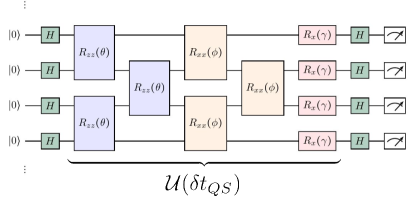
Figure 1: Quantum circuit employed for the quantum simulation. The gate parameters are given by $\theta=-2\delta t_{QS}J_{z}$, $\phi=-2\delta t_{QS}J_{x}$, $\gamma=-2\delta t_{QS}h_{x}$. The part implementing the evolution operator $\mathcal{U}(\delta t_{QS})$ is repeated $M$ times to reach the desired time $t$ (see text).

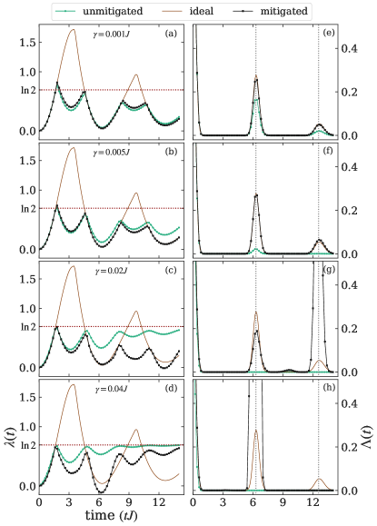
Figure 2: Rate function $\lambda(t)$ as a function of time for different depolarization noise levels, $\gamma$. We show the results for different re-scaling factors $\alpha$, as well as the extrapolated value to zero noise. Loschmidt echo $\Lambda(t)=e^{-N\lambda(t)}$ for depolarizing noise for different noise strength $\gamma$. We show the results for the ideal value and the extrapolated value to zero noise. For long-enough times and large-enough noise, the Loschmidt echo is bounded by a fully mixed state, which results in $\lambda=\ln{2}$, indicated by the red dashed line in each subplot.

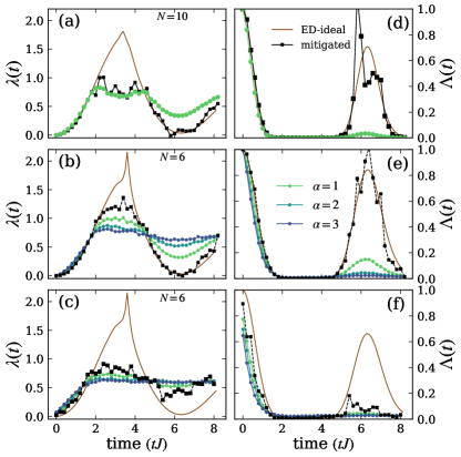
Figure 3: Quantum simulation results of the behavior of the rate function $\lambda(t)$ and the Loschmidt echo $\Lambda(t)$. (a,d) and (b,e) show the results using the depolarizing noise model with one-qubit error $p=0.001$, for $N=10$ and $N=6$ qubits, respectively. (c,f) show the simulation results with the noise model of the IBMQ Nairobi 7-qubit device. In all the figures we depict the exact diagonalization (ED) results, the unmitigated evolution, as well as the mitigated curve. In Figs. (b,e) and (c,f) we show as well the results for different noise scaling factors $\alpha$.

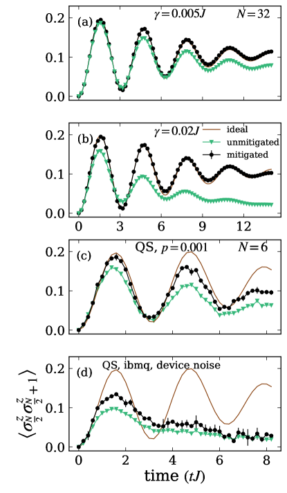
Figure 4: Two-point correlation $C_{zz}(t)=\langle\sigma_{\frac{N}{2}}^{z}\sigma_{\frac{N}{2}+1}^{z}\rangle$. (a, b) show MPDO simulations results for depolarizing noise with noise strength $\gamma$ for $N=32$. (c, d) shows the quantum simulator results for $N=6$ for $\alpha=1.0,1.5,2.0$. (c) shows the results for depolarizing noise channel with $p=0.001$ and (d) shows the results using the device noise of the IBMQ Nairobi. We show the results for the ideal, the unmitigated and the extrapolated value to zero noise.

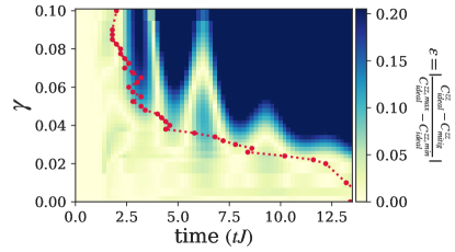
Figure 5: Error rate $\varepsilon=\left|\frac{C^{zz}_{\mathrm{ideal}}-C^{zz}_{\mathrm{mitigated}}}{C^{zz,max}_{\mathrm{ideal}}-C^{zz,min}_{\mathrm{ideal}}}\right|$ as a function of noise strength $\gamma$ and time $tJ$. The red curve shows the threshold $\varepsilon<0.04$, below which the simulation faithfully retrieves the dynamics of Model (1).

Loschmidt echo.–

Figure 2 shows the return rate $\lambda(t)$ for different values of $\gamma$ versus the ideal (noise-free) case. For a low noise $\gamma\leq 0.01J$, extrapolation recovers very well the ideal results, away from the DQPTs, all the way up to the maximal time considered $t=14/J$. For larger noise, ZNE may be significantly successful below a given noise and evolution-time threshold. In the right panels of Fig. 2 we show the Loschmidt echo $\Lambda(t)$. Note that ZNE recovers the first revival up to $\gamma=0.02J$, although for an unmitigated noise the revival is basically lost for $\gamma\gtrsim 0.005J$. For longer times and/or larger $\gamma$, ZNE fails eventually to recover, even qualitatively, the noise-free results. When accumulating noise, the system reaches a fully mixed state, $\rho_{s}(t)\equiv\frac{I}{2^{N}}$, such that $\operatorname{Tr}(\rho_{0}\rho_{s})\equiv\frac{1}{2^{N}}$ and the return rate is equivalent to $\lambda_{s}\rightarrow\ln{2}$.

The results in the vicinity of the DQPTs are considerably more affected by the noise. The expected peaks in $\lambda(t)$ associated to the DQPTs are not recovered even for a very low noise. Interestingly, for any noise, we observe rather a minimum of $\lambda(t)$, and hence a spurious revival of the Loschmidt echo, within the time window at which the DQPT occurs in the noise-free system. This minimum results from the noise-induced doubling of the non-analytic points of $\lambda(t)$, which seem to indicate noise-induced DQPTs. As a result, ZNE cannot recover (even qualitatively) the noise-free DQPT. This points to an inherent limitation of ZNE when applied to the quantum simulation of many-body dynamics.

Figure 3 shows our results obtained from the quantum simulator. For the case of depolarizing noise the results resemble those on the MPDO calculations (see Figs. 3 (a,d) and (b,e)). Note in particular that, as already observed in our MPDO calculations, using ZNE allows for the basically perfect recovery of the first revival of the Loschmidt echo, which is almost unobservable for the unmitigated case. Our quantum simulation results for up to $10$ spins, although significantly noisy in the DQPT region, suggest as well the doubling effect mentioned above (see Fig. 3(a)). The MPDO study of systems with variable number of spins indicate that the doubling, and the associated noise-induced spurious revival, become more prominent for a larger number of spins. Hence, finite-size effects may explain the differences with the MPDO results in the DQPT window.

In contrast, the device-noise simulations, see Figs. 3 (c,f), show that the noise strength in the considered device is large, and the results approach the fully-mixed state. As a result, ZNE can faithfully recover the exact results only for very short times ($t<2/J$), while failing at later times.

Two-site correlation.–

The analysis of the two-site correlation function in the middle of the spin chain, $C^{zz}(t)=\langle\sigma_{\frac{N}{2}}^{z}\sigma_{\frac{N}{2}+1}^{z}\rangle$, provides further information about the ZNE performance. The zero-noise evolution is characterized by oscillations of period $\pi/J$, which damp to a finite value. Figure 4 shows $C^{zz}(t)$ for different values of $\gamma$. We depict for each case the noise-free result $C_{\mathrm{ideal}}^{zz}(t)$, as well as the mitigated value $C_{\mathrm{mitigated}}^{zz}(t)$. For short times (shallow circuits), $Jt<2$, ZNE is successful for all $\gamma$ up to $0.1J$. For small values of the noise strength, $\gamma\leq 0.02J$, ZNE can recover the noise-free results up to the longest time considered. Note that, remarkably, this is so despite of the strong noise-induced damping observed already for $\gamma=0.005J$. For large $\gamma$ values noise results at long-enough times in a vanishing correlation, rendering the ZNE eventually unable to recover the noise-free result.

In Fig. 5, we depict the error rate, defined as $\varepsilon=\left|\frac{C^{zz}_{\mathrm{ideal}}-C^{zz}_{\mathrm{mitigated}}}{C^{zz,max}_{\mathrm{ideal}}-C^{zz,min}_{\mathrm{ideal}}}\right|$, as a function of both noise strength $\gamma$ and time $tJ$. Our results show a threshold, given by the red curve in Fig. 5, such that the ZNE is reliable below this threshold. In Fig. 5, for a given $\gamma$ we have determined the threshold time as that in which $\varepsilon<0.04$. One can, however, employ other thresholds that would provide a similar picture.

Our quantum simulation results for $N=6$, using depolarizing noise, confirm the significant improvement of the $C_{zz}(t)$ calculation when using ZNE (see Fig. 4 (c)). In contrast, ZNE produces a more modest improvement for the device-noise calculation (see Fig. 4 (d)).

Conclusions.–

We have investigated the performance of zero-noise extrapolation for the digital quantum simulation of the dynamics of many-body quantum systems. By means of matrix-product density operators, we have evaluated the particular case of the simulation of a quenched transverse-field Ising model in the presence of depolarizing noise. Our results show that zero-noise extrapolation allows to recover noise-free results, for both the Loschmidt echo and the inter-site correlation dynamics, below a given noise and evolution-time threshold. However, the method seems to be inherently unable to recover the ideal Loschmidt dynamics at dynamical phase transitions due to the appearance of a noise-induced revival. Our matrix-product density analysis, backed up by direct quantum simulations, provides a blueprint for the study of the performance of ZNE on noisy quantum processors with large number of qubits and deep circuits. Future work will address different noise models using the MPDO simulations for different quantum computing tasks, such as quantum optimization, and will benchmark these results with those on the actual device, developing a device-specific noise analysis. Another possibility would be to consider the role of cross-talks between qubits in the simulations and show how to mitigate them. Furthermore, one could expand such simulations to higher dimensions and a more realistic quantum chip geometry.

Supplemental Material: Quantum simulation of dynamical phase transitions in noisy quantum devices

We provide additional details and numerical results supplementing the conclusions from the main text.

I Matrix product density operators

The vectorized Liouvillian is given by

$$\mathcal{L}_{\#} \equiv-i(\mathcal{H}\otimes I-I\otimes\mathcal{H}^{T})$$

$$+\sum_{\mu}{(L_{\mu}\otimes L^{*}_{\mu}-\frac{1}{2}L^{\dagger}_{\mu}L_{\mu}\otimes I-\frac{1}{2}I\otimes L^{*}_{\mu}L^{T}_{\mu})}$$ (S1)

Fig. S1 shows different steps for MPDO time evolution

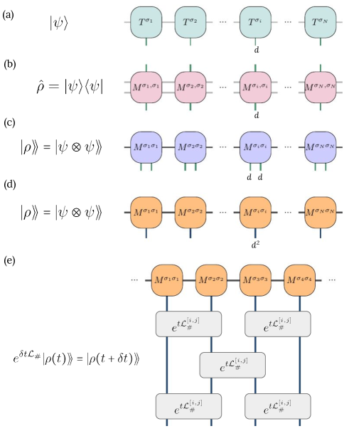
Figure S1: MPDO steps to evolve a system based on the Liouvilian master equation.

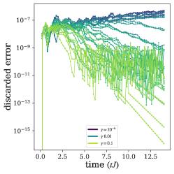
Figure S2: Discarded error of the MPDO simulation for the main results in the paper.

II Depolarizing noise channel

We comment in the following on the relation between the probabilistic error $p$ of the depolarizing channel, and the dissipation strength $\gamma$ in the Lindblad master equation:

$$\dot{\rho}=\gamma\sum_{\mu=x,y,z}\left(-\rho+\sigma^{\mu}\rho\sigma^{\mu}\right)=2\gamma(I-2\rho).$$ (S2)

Here we have employed the identity $\sum_{\mu}\sigma^{\mu}M\sigma^{\mu}=2\operatorname{Tr}(M)I-M$, valid for any $2\times 2$ matrix $M$, and $\operatorname{Tr}(\rho)=1$. Using the parametrization: $\rho(t)=\frac{1}{2}(I+\vec{r}(t)\cdot\vec{\sigma})$, we can rewrite the master equation in the form:

$$\dfrac{1}{2}\sum_{\mu}\dot{r}_{\mu}\sigma^{\mu}=-2\gamma\sum_{\mu}r_{\mu}\sigma^{\mu},$$ (S3)

and hence $r_{\mu}(t)=e^{-4\gamma t}r_{\mu}(0)$. Then:

$$\rho(\delta t)=\frac{1}{2}(I+e^{-4\gamma\delta t}\vec{r}(0)\cdot\vec{\sigma})=\left(1-p(\delta t)\right)\rho(0)+\frac{I}{2}p(\delta t),$$ (S4)

which has the form of a depolarizing channel with $p(\delta t)=1-e^{-4\gamma\delta t}$.

III Benchmarking the MPDO simulations vs exact diagonalization

In order to benchmark our MPDO results, we compare in the following the results obtained using exact diagonalisation and those from the MPDO calculation. We consider a small system site ($N=8$) and different noise strengths. We consider the integrable TFIM:

$$\mathcal{H}=\sum_{i}{(\sigma_{i}^{z}\sigma_{i+1}^{z}+h\sigma_{i}^{z})},$$ (S5)

with $J=1$ and $h=0.1$, and we quench from the same initial state as in the main text. Our results for the return rate depicted in Fig. S3 show an excellent agreement between exact diagonalization and MPDO calculations. Note also that compared to our MPDO calculations with $N=32$ sites, we do not observe for $N=8$ the same behavior within the DQPT region, which rather resembles more closely our quantum simulation results. This indicates that the differences in the main text between the quantum simulation and MPDO results in the vicinity of the DQPT are due to the different system sizes.

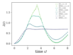
Figure S3: Dynamics of model (S5) for $N=8$ sites. Comparison of the return rate $\lambda(t)$ evaluated with exact diagonalization (ED) and with MPDO for different noise strengths. In our MPDO calculations we have employed a maximum bond dimension $\chi_{max}=200$.

IV Noise scaling in the quantum simulation

Noise scaling in gate-based quantum computation is based on unitary folding, which consists in replacing a unitary operation $U$ by $U\rightarrow U(U^{\dagger}U)^{n}$ with $n$ being a positive integer. As $U^{\dagger}U=I$, folding does not have any logical effect. However, the noise is increased with the prolongation of the circuit. The mitiq library is used to scale the quantum circuits for zero noise extrapolation. The scaling is done using folding at random introduced in LaRose et al. (2022); Giurgica-Tiron et al. (2020). Before scaling the circuits, one needs to transpile the quantum circuits using a set of universal basis gates, so that the depth of the circuit ran is precisely known; Here we have used basis gates $=[u1,~{}u2,~{}u3,~{}cx]$.

The value of the scaling factor $\alpha$ is important for the performance of ZNE. There are two options for unitary folding, circuit-folding and layer- or gate-based folding. The methods differ in the values of scaling factor $\alpha$ that can be reached. In circuit-folding the entire circuit is folded, and the values of $\alpha$ are of form $\alpha=1+2n$ where $n$ is the number of identities added. In order to get finer scaling, i.e. $\alpha$ being able to reach all real numbers, one can scale part of a circuit (folding only a selected number of layers from the entire circuit). The values of $\alpha$ are then of form $\alpha=1+(2k)/d$ where $k$ is any natural number and $d$ is the depth of the circuit. In this work we have employed layer-based folding. For more detailed information see Ref. Giurgica-Tiron et al. (2020).

References

- Nielsen and Chuang (2010) M. A. Nielsen and I. L. Chuang, Quantum Computation and Quantum Information: 10th Anniversary Edition (Cambridge University Press, 2010).
- Feynman (1982) R. P. Feynman, Int J Theor Phys 21, 467 (1982).
- Lidar. and Brun (2013) D. A. Lidar. and T. A. Brun, Quantum Error Correction (Cambridge University Press, 2013).
- Lloyd (1996) S. Lloyd, Science 273, 1073 (1996).
- Biamonte et al. (2017) J. Biamonte, P. Wittek, N. Pancotti, P. Rebentrost, N. Wiebe, and S. Lloyd, Nature 549, 195 (2017).
- Kandala et al. (2017) A. Kandala, A. Mezzacapo, K. Temme, M. Takita, M. Brink, J. M. Chow, and J. M. Gambetta, Nature 549, 242 (2017).
- Wendin (2017) G. Wendin, Rep. Prog. Phys. 80, 106001 (2017).
- Bruzewicz et al. (2019) C. D. Bruzewicz, J. Chiaverini, R. McConnell, and J. M. Sage, Applied Physics Reviews 6, 021314 (2019).
- Cirac and Zoller (1995) J. I. Cirac and P. Zoller, Phys. Rev. Lett. 74, 4091 (1995).
- Blatt and Roos (2012) R. Blatt and C. F. Roos, Nature Phys 8, 277 (2012).
- Jaksch et al. (1998) D. Jaksch, C. Bruder, J. I. Cirac, C. W. Gardiner, and P. Zoller, Phys. Rev. Lett. 81, 3108 (1998).
- Bloch et al. (2012) I. Bloch, J. Dalibard, and S. Nascimbène, Nature Phys 8, 267 (2012).
- Burkard et al. (2021) G. Burkard, T. D. Ladd, J. M. Nichol, A. Pan, and J. R. Petta, (2021), 10.48550/arXiv.2112.08863, comment: Rev. Mod. Phys. - Corrections and comments welcome, arXiv:2112.08863 [cond-mat, physics:physics, physics:quant-ph] .
- Slussarenko and Pryde (2019) S. Slussarenko and G. J. Pryde, (2019), 10.1063/1.5115814, comment: 21 pages, 3 figures. A brief review on some topics in photonic quantum computing with lots of references to longer specialist reviews. Close to published version, arXiv:1907.06331 [quant-ph] .
- Weedbrook et al. (2012) C. Weedbrook, S. Pirandola, R. García-Patrón, N. J. Cerf, T. C. Ralph, J. H. Shapiro, and S. Lloyd, Rev. Mod. Phys. 84, 621 (2012).
- Preskill (2018) J. Preskill, Quantum 2, 79 (2018).
- Temme et al. (2017) K. Temme, S. Bravyi, and J. M. Gambetta, Phys. Rev. Lett. 119, 180509 (2017).
- Endo et al. (2018) S. Endo, S. C. Benjamin, and Y. Li, Phys. Rev. X 8, 031027 (2018).
- Li and Benjamin (2017) Y. Li and S. C. Benjamin, Phys. Rev. X 7, 021050 (2017).
- van den Berg et al. (2022) E. van den Berg, Z. K. Minev, A. Kandala, and K. Temme, (2022), 10.48550/arXiv.2201.09866, arXiv:2201.09866 [quant-ph] .
- Mari et al. (2021) A. Mari, N. Shammah, and W. J. Zeng, Phys. Rev. A 104, 052607 (2021).
- Lowe et al. (2021) A. Lowe, M. H. Gordon, P. Czarnik, A. Arrasmith, P. J. Coles, and L. Cincio, Phys. Rev. Research 3, 033098 (2021).
- Takagi et al. (2022a) R. Takagi, S. Endo, S. Minagawa, and M. Gu, (2022a), 10.48550/arXiv.2109.04457, arXiv:2109.04457 [quant-ph] .
- Tsubouchi et al. (2022) K. Tsubouchi, T. Sagawa, and N. Yoshioka, (2022), 10.48550/arXiv.2208.09385, arXiv:2208.09385 [quant-ph] .
- Takagi et al. (2022b) R. Takagi, H. Tajima, and M. Gu, (2022b), 10.48550/arXiv.2208.09178, arXiv:2208.09178 [quant-ph] .
- Verstraete et al. (2004) F. Verstraete, J. J. García-Ripoll, and J. I. Cirac, Phys. Rev. Lett. 93, 207204 (2004).
- Zwolak and Vidal (2004) M. Zwolak and G. Vidal, Phys. Rev. Lett. 93, 207205 (2004).
- Cheng et al. (2021) S. Cheng, C. Cao, C. Zhang, Y. Liu, S.-Y. Hou, P. Xu, and B. Zeng, Phys. Rev. Research 3, 023005 (2021).
- Werner et al. (2016) A. H. Werner, D. Jaschke, P. Silvi, M. Kliesch, T. Calarco, J. Eisert, and S. Montangero, Phys. Rev. Lett. 116, 237201 (2016).
- Schollwöck (2011) U. Schollwöck, Annals of Physics 326, 96 (2011), january 2011 Special Issue.
- Urbanek et al. (2021) M. Urbanek, B. Nachman, V. R. Pascuzzi, A. He, C. W. Bauer, and W. A. de Jong, Phys. Rev. Lett. 127, 270502 (2021).
- Pfeuty (1970) P. Pfeuty, Annals of Physics 57, 79 (1970).
- Osborne and Nielsen (2002) T. J. Osborne and M. A. Nielsen, Phys. Rev. A 66, 032110 (2002).
- Heyl et al. (2013) M. Heyl, A. Polkovnikov, and S. Kehrein, Phys. Rev. Lett. 110, 135704 (2013).
- Heyl (2014) M. Heyl, Phys. Rev. Lett. 113, 205701 (2014).
- Heyl (2018) M. Heyl, Rep. Prog. Phys. 81, 054001 (2018).
- Heyl (2015) M. Heyl, Phys. Rev. Lett. 115, 140602 (2015).
- Karrasch and Schuricht (2013) C. Karrasch and D. Schuricht, Phys. Rev. B 87, 195104 (2013).
- Dborin et al. (2022) J. Dborin, V. Wimalaweera, F. Barratt, E. Ostby, T. E. O’Brien, and A. G. Green, Nat Commun 13, 5977 (2022).
- Halimeh and Zauner-Stauber (2017) J. C. Halimeh and V. Zauner-Stauber, Phys. Rev. B 96, 134427 (2017).
- Homrighausen et al. (2017) I. Homrighausen, N. O. Abeling, V. Zauner-Stauber, and J. C. Halimeh, Phys. Rev. B 96, 104436 (2017).
- Lang et al. (2018) J. Lang, B. Frank, and J. C. Halimeh, Phys. Rev. B 97, 174401 (2018).
- Van Damme et al. (2022a) M. Van Damme, J.-Y. Desaules, Z. Papić, and J. C. Halimeh, (2022a), 10.48550/arXiv.2210.02453, arXiv:2210.02453 [cond-mat, physics:quant-ph] .
- Van Damme et al. (2022b) M. Van Damme, T. V. Zache, D. Banerjee, P. Hauke, and J. C. Halimeh, (2022b), 10.48550/arXiv.2203.01337, arXiv:2203.01337 [cond-mat, physics:hep-lat, physics:quant-ph] .
- Jurcevic et al. (2017) P. Jurcevic, H. Shen, P. Hauke, C. Maier, T. Brydges, C. Hempel, B. P. Lanyon, M. Heyl, R. Blatt, and C. F. Roos, Phys. Rev. Lett. 119, 080501 (2017).
- Wu et al. (2022) L.-N. Wu, J. Nettersheim, J. Feß, A. Schnell, S. Burgardt, S. Hiebel, D. Adam, A. Eckardt, and A. Widera, (2022), 10.48550/arXiv.2208.05164, arXiv:2208.05164 [cond-mat, physics:quant-ph] .
- Kandala et al. (2019) A. Kandala, K. Temme, A. D. Córcoles, A. Mezzacapo, J. M. Chow, and J. M. Gambetta, Nature 567, 491 (2019).
- Endo et al. (2021) S. Endo, Z. Cai, S. C. Benjamin, and X. Yuan, J. Phys. Soc. Jpn. 90, 032001 (2021).
- Giurgica-Tiron et al. (2020) T. Giurgica-Tiron, Y. Hindy, R. LaRose, A. Mari, and W. J. Zeng, in 2020 IEEE International Conference on Quantum Computing and Engineering (QCE) (2020) pp. 306–316.
- LaRose et al. (2022) R. LaRose, A. Mari, S. Kaiser, P. J. Karalekas, A. A. Alves, P. Czarnik, M. E. Mandouh, M. H. Gordon, Y. Hindy, A. Robertson, P. Thakre, M. Wahl, D. Samuel, R. Mistri, M. Tremblay, N. Gardner, N. T. Stemen, N. Shammah, and W. J. Zeng, Quantum 6, 774 (2022).
- Burden and Faires (2010) R. L. Burden and J. D. Faires, Numerical Analysis (Cengage Learning, 2010).
- Montangero (2018) S. Montangero, Introduction to Tensor Network Methods: Numerical Simulations of Low-Dimensional Many-Body Quantum Systems (Springer International Publishing, Cham, 2018).
- Javanmard et al. (2018) Y. Javanmard, D. Trapin, S. Bera, J. H. Bardarson, and M. Heyl, New J. Phys. 20, 083032 (2018).
- Cirac et al. (2021) J. I. Cirac, D. Pérez-García, N. Schuch, and F. Verstraete, Rev. Mod. Phys. 93, 045003 (2021).
- Hatano and Suzuki (2005) N. Hatano and M. Suzuki, Quantum Annealing and Other Optimization Methods, Lecture Notes in Physics, 37 (2005).
- IBM-Quantum (2021) IBM-Quantum, “Qiskit: An open-source framework for quantum computing,” (2021).
- Smith et al. (2019) A. Smith, M. S. Kim, F. Pollmann, and J. Knolle, npj Quantum Information 5, 106 (2019).
- Fauseweh and Zhu (2021) B. Fauseweh and J.-X. Zhu, Quantum Inf Process 20, 138 (2021).