Forecasting Bitcoin volatility spikes from whale transactions and CryptoQuant data using Synthesizer Transformer models

Abstract

The cryptocurrency market is highly volatile compared to traditional financial markets. Hence, forecasting its volatility is crucial for risk management. In this paper, we investigate CryptoQuant data (e.g. on-chain analytics, exchange and miner data) and whale-alert tweets, and explore their relationship to Bitcoin’s next-day volatility, with a focus on extreme volatility spikes. We propose a deep learning Synthesizer Transformer model for forecasting volatility. Our results show that the model outperforms existing state-of-the-art models when forecasting extreme volatility spikes for Bitcoin using CryptoQuant data as well as whale-alert tweets. We analysed our model with the Captum XAI library to investigate which features are most important. We also backtested our prediction results with different baseline trading strategies and the results show that we are able to minimize drawdown while keeping steady profits. Our findings underscore that the proposed method is a useful tool for forecasting extreme volatility movements in the Bitcoin market.

[label1]organization=SUTD,addressline=Somapah Road 8, city=Singapore, postcode=487372, state=Singapore, country=SG

We propose a new Synthesizer Transformer model to predict next-day BTC volatility.

Our predictive model takes as input whale-alert data from Twitter.

Our model also uses CryptoQuant data, which includes on-chain and exchange data.

Explainable AI techniques (XAI) are used to uncover important features.

Basic trading strategies show that the volatility predictions can reduce risk.

1 Introduction

This paper studies the most popular cryptocurrency, Bitcoin, which is currently traded on more than 500 exchanges. Since Bitcoin is the first cryptocurrency, established in 2008 (Nakamoto, 2008), it provides the longest historical data to study. Compared to traditional financial instruments like equities and commodities, cryptocurrencies like Bitcoin have large, so-called ‘whale’ holders, which consist of about 1,000 people who own around 40% of the market (Kharif, 2017). In this paper, we explore how large Bitcoin transactions from these whales affect the market volatility. We propose a state-of-the-art deep learning Synthesizer Transformer model (Tay et al., 2020) that predicts if Bitcoin’s volatility will be extreme the next day, based on transaction data from these whales as well as a variety of features from CryptoQuant, including on-chain metrics, miner flows, and more. We compare this proposed model with existing baseline models and propose a simple trading strategy to demonstrate the practical usefulness of the predictions. In our experiments, we also analyse the importance of the different CryptoQuant and whale-alert features that most influence volatility. An overview of our paper is provided in Figure 1. The code of our proposed (trained) models is made available online.

Figure 1: Overview of the proposed study.

We focus on the volatility of Bitcoin as this digital asset dominates the cryptocurrency market with the largest market cap after USDT. In finance, volatility refers to the degree of variation of an asset’s price over time (Black et al., 2012). Market volatility is generally considered a vital metric to evaluate the level of risk, and thus it plays a critical role in assessing the stock market risk and the pricing of derivative securities (Yang et al., 2020). Compared to traditional financial instruments, the price of Bitcoin is highly volatile (Blau, 2017). In general, the Bitcoin market is currently highly speculative, and thus more susceptible to speculative bubbles than other traditional currency markets (Grinberg, 2012; Cheah and Fry, 2015). Bitcoin has recently also found its place in portfolios to hedge against the global geopolitical crisis (Dyhrberg, 2016) and reduce financial market uncertainty ((Platanakis and Urquhart, 2019; Fang et al., 2019; Colon et al., 2021), hence studying risk and assessing exposure is important to cryptocurrency investors, and it becomes important to model and forecast the volatility of Bitcoin. In this paper, we focus on predicting future spikes in Bitcoin’s volatility.

This study aims to gain further insights into the market conditions that may cause drastic increases in volatility in Bitcoin markets. Our contribution is threefold. We first thoroughly explore both CryptoQuant data and the influence of whale transactions on volatility. Second, we propose and evaluate a state-of-the-art Synthesizer Transformer model to predict volatility. Finally, we propose a basic trading strategy that leverages the volatility predictions to reduce downward risk. We briefly touch upon the importance of these contributions in what follows.

First, in this study, we gather a dataset from CryptoQuant, as well as whale transaction tweets from January 2018 to September 2021. The former includes information such as exchange and miners transactions as well as liquidations and open interest caused by trading with leverage (full feature set, see Table LABEL:tab:cryptoquant_table). We thoroughly explore the relationship between this data and Bitcoin’s next-day volatility, and focus on discovering large market movements induced by the ripple effects of large whale transactions and on-chain movements.

Second, we propose a Synthesizer Transformer model to perform the volatility spike prediction. The Transformer architecture has proven to be extremely efficient for a range of tasks related to time series such as text translation (Vaswani et al., 2017), music generation (Makris et al., 2021), emotion prediction from movies (Thao et al., 2021), and speech synthesis (Li et al., 2019). In finance, it has been shown to be efficient at stock price (Liu et al., 2019; Zhang et al., 2022) and even stock volatility prediction (Yang et al., 2020). In the cryptocurrency markets, we see that it has been used for Dogecoin (Sridhar and Sanagavarapu, 2021) and Bitcoin (JAIN, 2019) price prediction. In this work, we expand the existing literature by including CryptoQuant and whale data (plus technical indicators calculated on this data). We then go beyond just building a black-box model, but also explore the influence of these features on volatility prediction through explainable artificial intelligence (XAI) techniques with the Captum library (Kokhlikyan et al., 2020). Instead of using Vanilla (standard) Transformer architectures, we change the typical dot product self-attention mechanism to Synthesizer attention, which learns synthetic attention weights without token-to-token interactions. By doing so, we optimize the attention span of the model. Recent work has shown that Synthesizer Transformers outperform traditional Transformers. Even a simple Random Synthesizer has shown to be 60% faster than a traditional Transformer (Tay et al., 2020). In an experiment, we compare our proposed architecture to other configurations and baseline traditional models like GARCH. We show that it is a useful and reliable method for forecasting volatility in cryptocurrencies.

Finally, we explore the usefulness of our predictions by backtesting a number of trading strategies that use the predicted volatility. In practice, investors often use volatility to trade derivative instruments such as put and call options (Ni et al., 2008). Since it is hard to backtest such a strategy in a Bitcoin context, we propose examples of simple trading strategies which use trading signals based on our volatility prediction model. We explore four different strategies: buy & hold, buy-low-sell-high, mean reversion and momentum-based. When we include position scaling based on volatility, we notice an increase in the cumulative returns as well as the Sharpe ratio. In future work, these strategies should further be improved, but for now, they serve as a simple example that our prediction model can be used to lower the downside risk of a portfolio.

The rest of this paper is structured as follows. In Section 2, we review the existing literature, followed by a thorough description and visualisation of the dataset that was collected. Next, the proposed Synthesizer Transformer models are introduced in Section 4. Section 5 provides a detailed account of the performance of the volatility prediction models compared to benchmarks, as well as insight into the important features through XAI. The setup and results of the backtesting experiment is described in Section 6. Finally, we provide conclusions and suggestions for further work in Section 7.

2 Literature Review

We provide a brief overview of literature related to on-chain data, using Twitter data for volatility and price prediction, followed by deep models for cryptocurrency-related predictions. For a more complete overview, the reader is referred to (Zou and Herremans, 2022; Charandabi and Kamyar, 2021; Khedr et al., 2021; Charandabi and Kamyar, 2022).

2.1 Cryptocurrency-specific data

The cryptocurrency markets are fundamentally quite different from traditional stock markets. One of the key differences is the transparency provided by blockchain technologies (Biswas and Gupta, 2019). Transparency is one of the key features of Bitcoin trading as the entire trading history is available and traders are provided with information on the complete state of the order book, but trading itself is pseudonymous. This transparency provides unique features that may be useful for price and volatility prediction.

On-chain data includes information from the blockchain ledger, such as the details of each transaction (e.g. from which wallet, to which wallet, amount, fees paid to miners), and the difficulty of mining blocks as well as the block sizes (Jagannath et al., 2021; Kim et al., 2022). The availability of such data can gives us incredible insight in upcoming price movements (Zheng et al., 2021). The transparency in the blockchain even allows us to access the entire transaction history ever recorded. There is no hidden volume (as in iceberg orders) nor dark pools (Dimpfl, 2017). However, to use this data would require a huge amount of computing power, hence, we focus on aggregated on-chain data instead. CryptoQuant provides us with a wide selection of such features, and also includes exchange data such as the amount of liquidations, as well as data on Bitcoin miners.

Looking at existing literature, we see that utilizing this transparency allows one to establish a trader’s edge. For instance, Kim et al. (2022) show that on-chain data can be useful when predicting Bitcoin’s price with a self-attention-based multiple long short-term memory model (SA-LSTM). While they provide a list of 42 variables used, there is no ablation study or XAI method used to identify which variables are most important. Jagannath et al. (2021) equally show that the Ethereum price can be predicted using on-chain data and a self-adaptive LSTM model. A correlation analysis using their data reveals important correlated on-chain features to the price of Ethereum. These features include transaction rate, supply in smart contracts, block difficulty and hash rate.

On-Chain data is not only useful for price prediction, the correlation between on-chain transaction activities and volatility has been shown by Gkillas et al. (2021). Raheman et al. (2021)’s developed agent for crypto-portfolio management also uses on-chain data for price trend and volatility prediction. The literature available on the effects of various cryptocurrency-specific data such as on-chain data is still in its early shoes. In this work, we aim to not just build a predictive model for volatility, but also thoroughly analyse the patterns within the data and provide an XAI interpretation of the resulting model.

In addition to CryptoQuant data, we also parsed a new dataset of whale transactions. An overview of the literature related to this is provided in the next subsection.

2.2 Importance of Twitter data for volatility

The CryptoQuant data offers us nice insights into aggregated on-chain data, miner data and more. It does not, however, include transactions by so-called ‘crypto-whales’, holders of very large wallets. It is well known that cryptocurrencies are very volatile in nature, thus creating both outstanding benefits as well as a huge risk to investors (Bariviera et al., 2017; Klein et al., 2018). Part of this volatility can be attributed to large (whale) transactions and their ripple effect on the market. In this work, we will be using very specific Twitter content, namely ‘whale-alert’ tweets. The Twitter account@whale_alert, is a third-party information provider that “monitors millions of daily cryptocurrency transactions and publishes notable events on Twitter in near real-time” (Saggu, 2022). Scaillet et al. (2020) found a correlation between their ‘whale index’ and high-frequency price jumps of Bitcoin.

Social media sources such as Twitter have been shown to be helpful data sources for stock or cryptocurrency price predictions. To name a few examples, Lamon et al. (2017) study whether including sentiment analysis of news and social media can improve models when predicting the price of Bitcoin and Ethereum. Aharon et al. (2022) explore the relationship between two novel Twitter-based measures of economic and market uncertainty and the performance of four major cryptocurrencies. Zou and Herremans (2022) shows that using BERT context embeddings of tweets with an LSTM model can improve Bitcoin price prediction. News and social media data have also been shown to be useful for volatility prediction, as Sapkota (2022) predicts Bitcoin volatility based on news sentiment, and Akbiyik et al. (2021) use temporal convolutional neural networks for Bitcoin volatility prediction with Twitter sentiment. Shen et al. (2019) show that the number of tweets is a major determinant of the next day’s trading volume and realised volatility of Bitcoin. Finally, Wu et al. (2021) reported that there is a significant Granger-causality from Twitter-based uncertainty measures to Bitcoin, Ethereum, Litecoin, and Ripple prices in different time periods. In this work, we will focus on integrating tweets by @whale_alert into our Transformer model.

2.3 Deep neural networks for financial time series predictions

Traditional models, like Generalised autoregressive conditional heteroscedasticity (GARCH)-based models) are widely used for volatility forecasting (Engle, 1982; Bollerslev, 1986). Katsiampa (2017) and Bergsli et al. (2022) study volatility forecasting for Bitcoin using GARCH and its variants. Naimy and Hayek (2018) concluded, however, that the predictive ability of GARCH is not good in the context of unusually high volatility, and performs better when volatility is relatively low. Vilasuso (2002) brings up one of GARCH’s major limitations where “its memory is sometimes not long enough to capture the persistence of some shocks that are observed to last for a very long time”. Jiang et al. (2022) propose a time-varying mixture model, which includes an accelerating generalized autoregressive score (aGAS) technique into the Gaussian-Cauchy mixture (TVM)-aGAS model for forecasting Value-at-Risk for cryptocurrencies. Recently, however, many researchers have turned to ever more powerful deep learning models for financial time series prediction.

Just like in the stock market (Ding et al., 2015; Hu et al., 2021; Jiang, 2021), deep learning models have become popular tools for price prediction in cryptocurrency markets (Zou and Herremans, 2022; Yao et al., 2018; Patel et al., 2020; Akyildirim et al., 2021; Alessandretti et al., 2018; Khedr et al., 2021). Looking at time series in general, recurrent neural networks, such as long-short term memory models (LSTMs) (Hochreiter and Schmidhuber, 1997) and gated recurrent unit (GRUs) (Chung et al., 2014) have been widely used for forecasting. When it comes to volatility prediction, Vidal and Kristjanpoller (2020) proposed an architecture based on convolutional neural networks (CNNs) and long-short term memory (LSTM) units to forecast gold volatility. LSTMs were also used by Jung and Choi (2021) to forecast currency exchange rate volatility. Finally, temporal convolutional neural networks have been used with Twitter sentiment data to predict Bitcoin volatility (Akbiyik et al., 2021).

In recent years, with the invention of the Transformer network (Vaswani et al., 2017), deep models for time series prediction have become even more powerful. Transformers use a self-attention mechanism, to give relative focus on the context of an element of a time series, and are better able to capture long-term trends. In finance, we have seen the successful use of Transformer architectures for tasks such as stock price prediction (Ding et al., 2020), stock volatility prediction (Ramos-Pérez et al., 2021), and even cryptocurrency price prediction such as Dogecoin (Sridhar and Sanagavarapu, 2021) and Bitcoin (JAIN, 2019). The work on volatility prediction for Bitcoin with Transformers is relatively non-existent, except for the work by Sapkota (2022) who built a model based on Twitter sentiment data. In this work, we explore how we can use the powerful Transformer architecture to perform Bitcoin volatility prediction, not only based on candlestick data, but also CryptoQuant data and whale-alert tweets. In addition, we implement the Synthesizer Transformer, to further optimize the attention mechanism.

3 Dataset collection and analysis

The Bitcoin market provides interesting conditions from a volatility point of view. There is 24-hour continuous trading, 365 days a year, with a lack of central authorities (e.g., central banks), resulting in the absence of a volatility trading halt, and no pre-market/post-market trading as compared to the equities market (Brandvold et al., 2015). These market conditions, along with the complete transparency of the on-chain trading data, create an interesting opportunity for us to study the influence of different factors on volatility. To do so, we have gathered a dataset from January 2016 until September 2021, which consists of CryptoQuant (on-chain data and market data from cryptocurrency exchanges), and whale transaction tweets. We will start below by discussing the features in this dataset and how we gathered them, and then move on to include technical indicators and data preprocessing.

3.1 Data sources

In this section, we discuss how we gathered whale transaction data which includes many aspects such as whale accumulation, whale dumping, miners’ inflow and outflow, as well as exchanges’ inflow and outflow.

3.1.1 Whale-alert data

Crypto ‘whales’ include some of the largest wallet holders, and hence have a significant influence on both price and volatility (Nguyen et al., 2018). In any volatility model, it is thus essential to include data about whale transactions. In order to do so, we tracked the Twitter handle @whale_alert, which provides continuous alerts as whale transactions happens. Some example tweets by this handle are shown below:

• “997 #BTC (6,269,280 USD) transferred from #Bitfinex

  to Unknown wallet”

• “11,000 #ETH (2,473,411 USD) transferred from Unknown

  wallet to #Gemini”

• “6,000,000 #USDC (6,000,000 USD) burned at USDC Treasury”

Once we collected all of the tweets from 12 September 2018 (earliest available) to 18 October 2021, we filtered transactions using the hashtag #BTC and the keyword ‘transferred’, resulting in a total of 52,787 tweets. We then wrote a parser that uses a set of rules to obtain useful data from these tweets such as total daily inflow and outflow of wallet to exchange, e.g. the word after ‘from’ will be the source of transaction and the word after ‘to’ will be the destination. For all of the tweets gathered in a day, we determine the overall net transaction outflow or inflow of wallets to exchanges in one day, resulting in the following daily features:

BTCminus

The amount of Bitcoin flowing out of wallets into exchanges.

BTCplus

The amount of Bitcoin flowing into wallets from exchanges.

USDminus

The amount of USD flowing out of wallets into exchanges.

USDplus

The amount of USD flowing into wallets from exchanges.

This data is relevant for our task: a transaction from wallet to exchange typically indicates a bearish sentiment given that the seller is closing their Bitcoin position and may want to exchange it into fiat currency. On the other hand, a transaction from exchange to wallet means that a buyer is planning to keep their Bitcoin position (or at least not exchange it into fiat) and is therefore bullish. For the purpose of this study, we only examine Bitcoin transactions that flow either from exchange to wallet or wallet to exchange. The total net flow of transactions from wallet to wallet and exchange to exchange is ignored.

Figure 2 plots the BTC price volatility against the number of BTC transactions measured in the daily amount of BTC that flowed to and from exchanges as per our whale-alert tweets. We see that there are patterns where volatility spikes during a spike in BTC transactions. There are 330 volatility spikes in total and we see that the net daily amount of BTC that flowed to or from exchanges (calculated as $abs(\text{BTCplus}-\text{BTCminus})$) has a Pearson correlation of 0.47 with daily BTC price volatility.

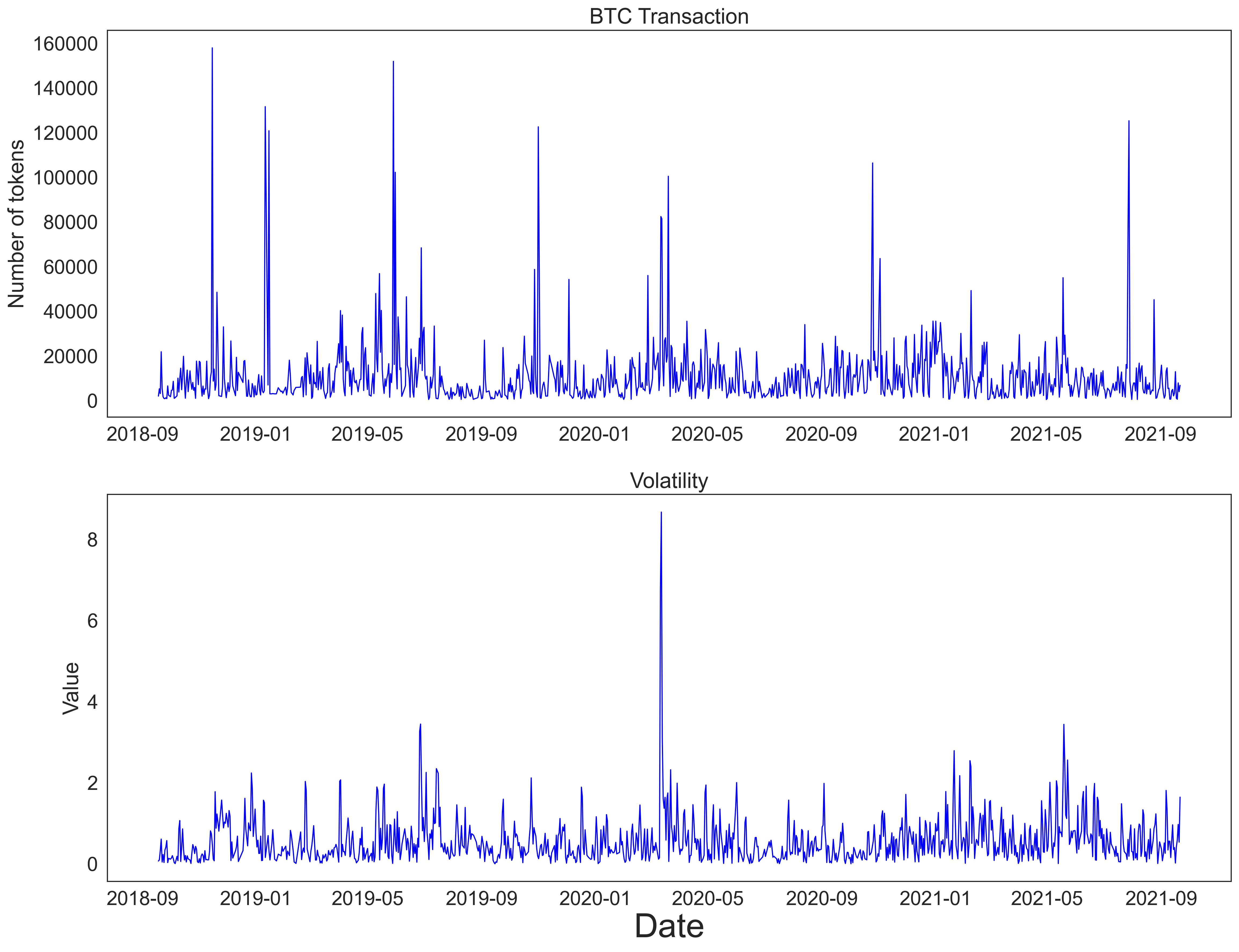
Figure 2: The daily amount of net BTC that flowed to or from exchanges per day, calculated as $abs(\text{BTCplus}-\text{BTCminus})$ (top). The BTC price volatility (bottom).

3.1.2 CryptoQuant on-chain and exchange data

CryptoQuant data provides comprehensive on-chain and market data gathered from both the blockchain as well as major cryptocurrency exchanges. Every single transaction that occurs in these markets is tracked by CryptoQuant. CryptoQuant even keeps track of which addresses are exchanges or mining pools, and aggregates the amount of BTC flowing between different types of entities, such as miners, and exchanges. In this study, we use CryptoQuant’s API to gather BTC related data. While a full overview of all the features we use is provided in Table LABEL:tab:cryptoquant_table based on CryptoQuant’s documentation, we elaborate on a few specific examples below:

miner_inflow_mean_ma7

The 7-day moving average of miner inflow gives us insight into when whale accumulation occurs. Miners are often considered to be the original whales, as they typically hold large wallets.

mtoe_flow_total

The miners-to-exchanges feature will keep track of how much BTC miners are transferring to exchanges. Typically, the main reason to send Bitcoin to an exchange would be to sell it, hence this can be a bearish indicator.

miner_outflow_top10

The amount of Bitcoin that flows out of the 10 largest Bitcoin wallets held by miners. These whale wallets will be responsible for downward pressure and increased volatility if this variable increases.

long_liquidation

The amount of leveraged positions in BTC that were forced to exit due to volatility. High values for this variable hence often go hand in hand with high volatility.

3.2 Technical Indicators

In order to improve the prediction of our volatility prediction model, we include some traditional technical indicators as input which have shown to be correlated to volatility (Liashenko et al., 2020). These include Exponential Moving Average (EMA), High-Low Spread, and Close-Open Spread. Exponential moving average indicators place a higher weighting on recent data compared to old data, hence, they are more reactive to the latest price changes compared to simple moving averages (SMAs). For this reason, we chose to include the 10th day EMA of the closing price instead of its SMA. This was calculated as per the below Equation 1 whereby $n$ is the number of days over which the EMA at time $t$ for a time series $X$ is calculated. The variable $S$ represents a smoothing factor, which we set to 2 for our study.

$$\text{EMA}_{t}=X_{t}\times(\frac{S}{1+n})+\text{EMA}_{t-1}\times(1-\frac{S}{1+n})$$ (1)

A second technical indicator is the High-Low Spread. This indicator gives insight into the intra-day total price movement. A higher value means that the price fluctuated in either direction in one day, thus indicating a higher volatility for that day, and vice versa.

$$\text{High-Low Spread}=\frac{\text{High}-\text{Low}}{\text{Close}}$$ (2)

Finally, the Open-Close indicator provides a sense of the direction and size of the move. If the price goes up, this indicator will be negative, and vice versa.

$$\text{Close-Open Spread}=\frac{\text{Close}-\text{Open}}{\text{Open}}$$ (3)

3.3 Data preprocessing

3.3.1 Missing values

Some of the used technical indicators, such as exponential moving average, have a short warm-up period resulting in missing values. We can fill up the missing values by using the first available value since this only occurs at the very beginning of our (training) dataset.

The whale exchange tweets and derivatives data were only available from 2018 onwards. Before that period, we consider them to be zero. For leverage and derivatives data, it is easy to assume that the missing values are 0 since these assets were not yet available or created.

3.3.2 Standardization

Some of the distributions of the input features are skewed which would affect the Transformer’s predictive abilities, hence we set out to standardize this. The descriptive statistics of features in Table LABEL:tab:before_normalization are standardized in Table LABEL:tab:after_normalization. Depending on how the data was skewed, we used five different techniques to standardize them as much as possible, as summarised in the latter table. We perform no change to features that are left skewed or that have a skewness less than 0.5 close to 0. As a default, for features with a higher right skewness (>0.5), we will perform a log() transform. In some cases, this can result in negative values, more specifically when the original values are <1, hence we cannot simply apply log(). We discuss the cases in which that happened and how we accounted for this:

• MVRV, miner_inflow_mean_ma7 and exchange_mean_ma7 have a skewness of 0.875, 1.55, and 1.16. Since all three of them have values in the range of 0.6 to 4, taking the logarithm would introduce negative values, therefore, we took the square root.

• The features HL_sprd, miner_inflow_mean, exchange_inflow_mean, exchange_outflow_mean and miner_outflow_mean, have a higher maximum value (>5) and skewness (>3). Hence, we perform a slightly stronger transformation and take the cube root, so as the make the maximum values closer to 1.

• Both the etom_flow_mean and mtoe_flow_mean features have a high skewness value of 17.19 and 20.48. Since their minimum value is below 1 (0.0769 and 0.298), we first add a value of 1 to them and then take the logarithm.

• For the feature vol_future, we took the power of $\frac{1}{4}$, to make the maximum value of 8.67 as close to 1 (threshold value) as possible. Given that this is our forecast variable, it was important to standardize this as good as possible.

3.4 Volatility

3.4.1 Calculating volatility

We calculated the daily volatility $V_{annualised}$ for our dataset using the formula below.

$$log-returns=x_{i}=ln(\frac{C_{i}}{C_{i-1}})$$ (4)

$$V_{annualised}=\sqrt{\frac{\sum\limits_{i=1}^{N}(x_{i}-\mu)^{2}\times 365}{N}}$$ (5)

where:

$$\textit{$\mu$}=\text{mean of log-returns}$$

$$\textit{$C_{i}$}=\text{closing price of day $i$}$$

$$\textit{$C_{i-1}$}=\text{closing price of day $i-1$}$$

$$\textit{$N$}=\text{number of days}$$

As shown in Figure 3, the daily volatility in our dataset is in the range of 0.000234 to 8.67. This results in a long-tailed distribution (see Figure 4) with a skewness of 3.35. Since statistical learning models typically work better with normally distributed data, we apply a transformation to the volatility data by taking the power of $\frac{1}{4}$. This results in a distribution with a skewness of -0.001 and a volatility range of volatility of 0.124 to 1.72.

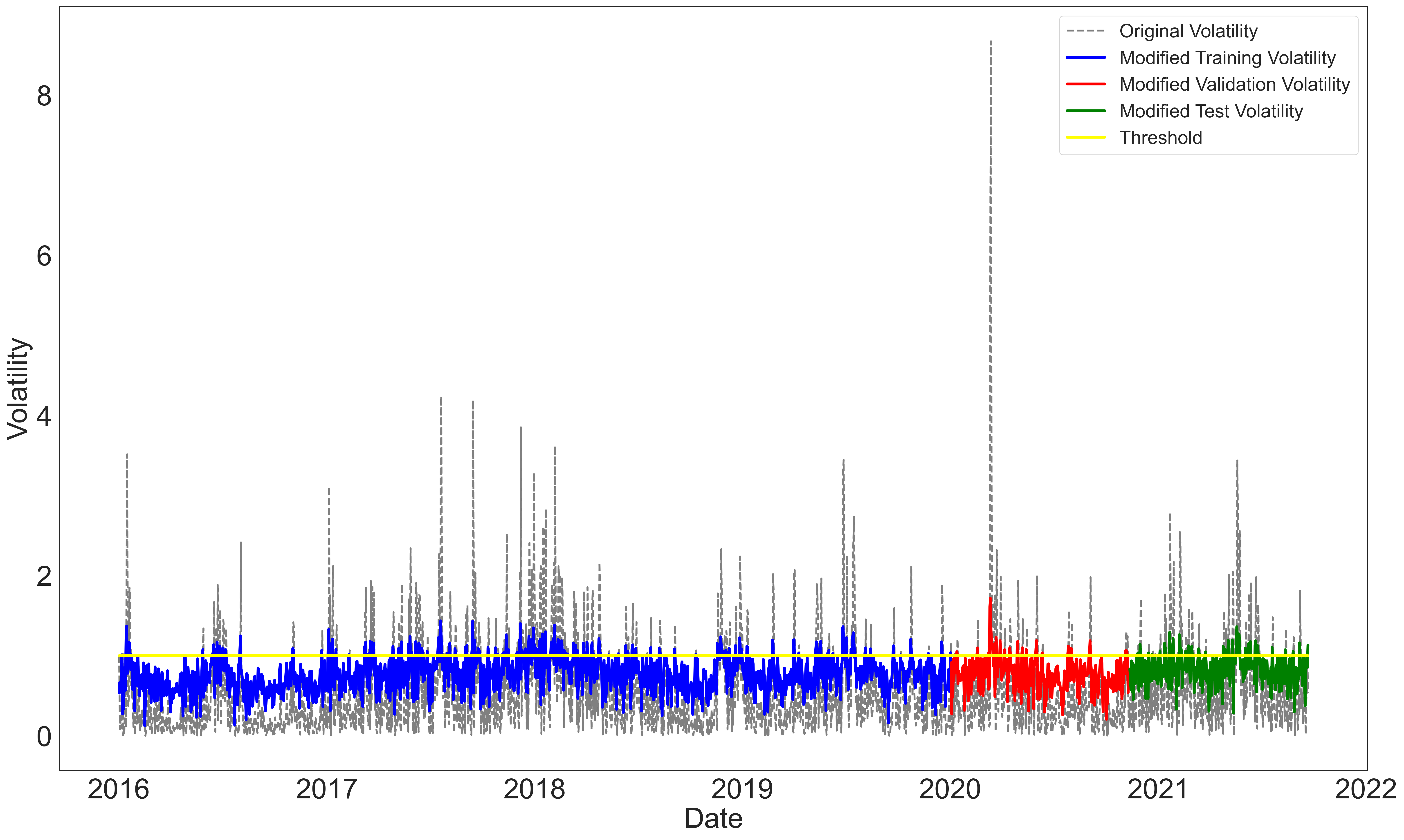
Figure 3: Daily Volatility before and after transformation.

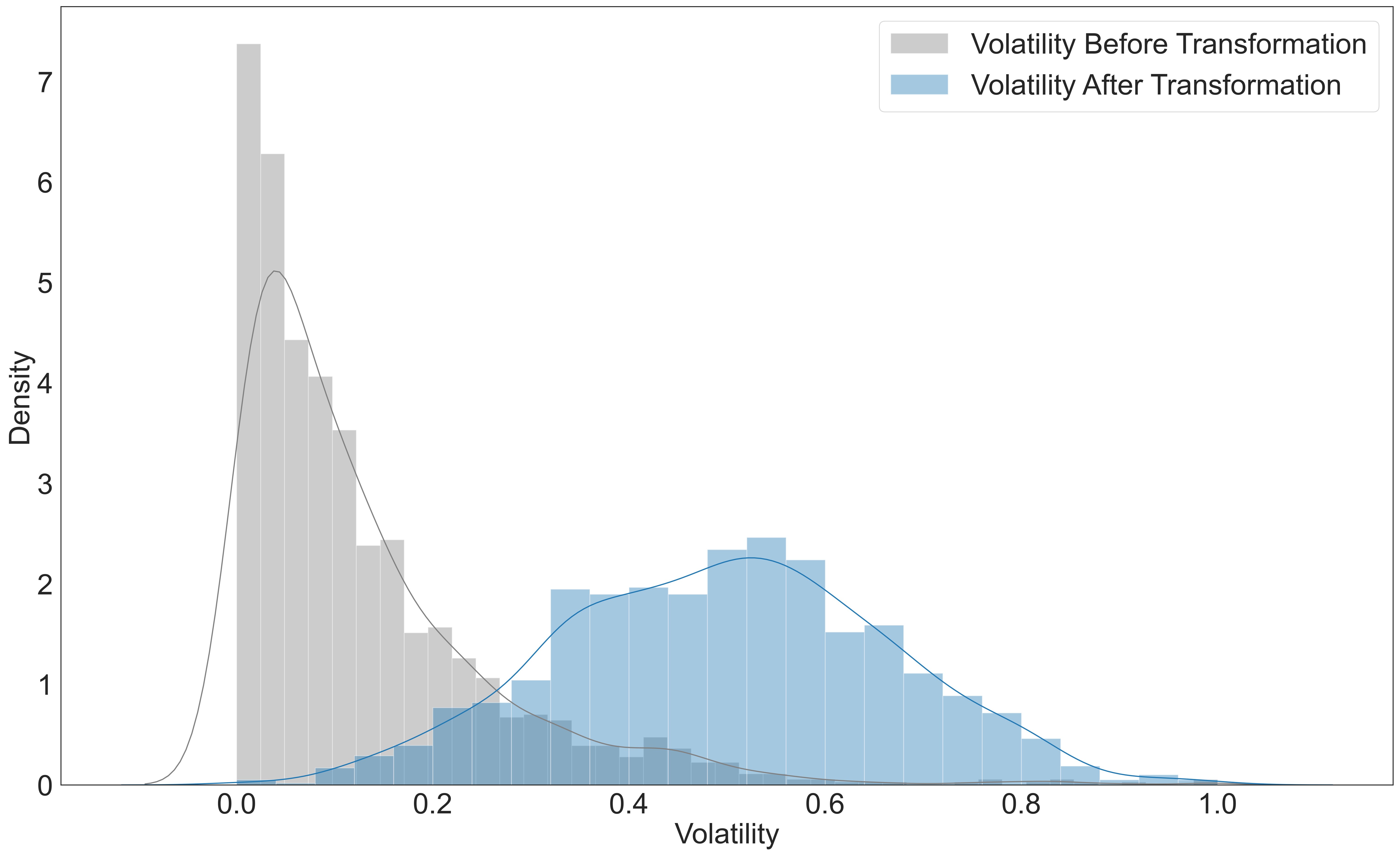
Figure 4: Volatility distribution before and after transformation.

3.4.2 Volatility spikes

As shown in Figure 3, we classify days with a volatility $\geq$ 1.0 and with positive log-returns of the closing price as a volatility spike. We set this volatility threshold to 1, because after applying the preprocessing transformation to the volatility (taking the power of $\frac{1}{4}$), all of the high volatilities with a magnitude > 1 will still be greater than 1 even though their magnitude has shrunk, and all of the low volatilities with a magnitude < 1 will still remain < 1. There are 232 volatility spikes in the training set and 38 volatility spikes in the validation set. In the test set, there are 60 volatility spikes.

3.4.3 Feature correlation with volatility

To explore which of the (input) features from our dataset may be most correlated with the next-day volatility, and thus most important for our predictive model, we calculated several correlation metrics. Table LABEL:tab:corr shows the R², and the Pearson as well as the Spearman correlation coefficients. We can see from the table that some features, such as volume, exchange_inflow_total and High_Low_Spread show a high correlation with the volatility. This indicates that these features will likely be important to improve our model’s predictive power. This will later be verified by doing a Captum analysis in Section 5 to explore the importance of each feature in our predictive model.

4 Proposed Synthesizer Transformer

In this paper, we leverage a new type of Transformer, the Synthesizer Transformer (Tay et al., 2021). To properly understand our architecture, we first provide an overview of the Vanilla Transformer architecture upon which our proposed model is based.

4.1 Transformer architecture

The architecture used in this paper draws inspiration from the Generative Pre-trained Transformer 2 (GPT-2)’s decoder-only Transformer (Radford et al., 2018), as shown in the Figure 5(a). In this architecture, the input to the Transformer is a multivariate time series. The decoder takes the masked target sequence so that at each time step the decoder can attend to the previous $i$ time steps. This is illustrated in Figure 5(b) where the first input $X_{1}$ will result in a prediction for the next time step: $X_{2}$’. In the next step, the decoder is given the ground truth $X_{1}$ and $X_{2}$ values to predict $X_{3}$’ and so forth. Therefore, at every new step, the model receives all the true inputs prior to predicting its next output, whereby each output token contributes equally to the training loss.

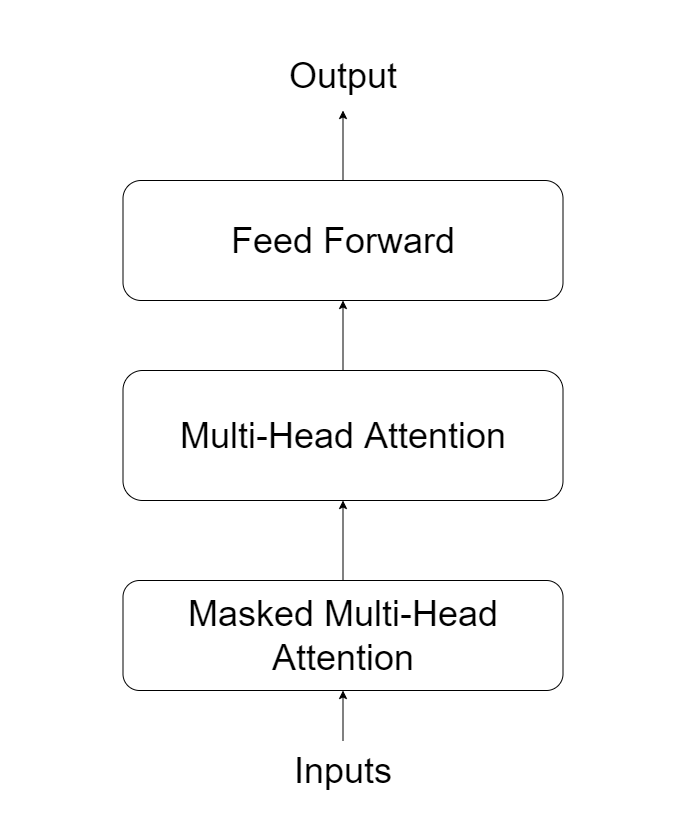
(a) The proposed decoder-only Transformer architecture inspired by (Radford et al., 2018).

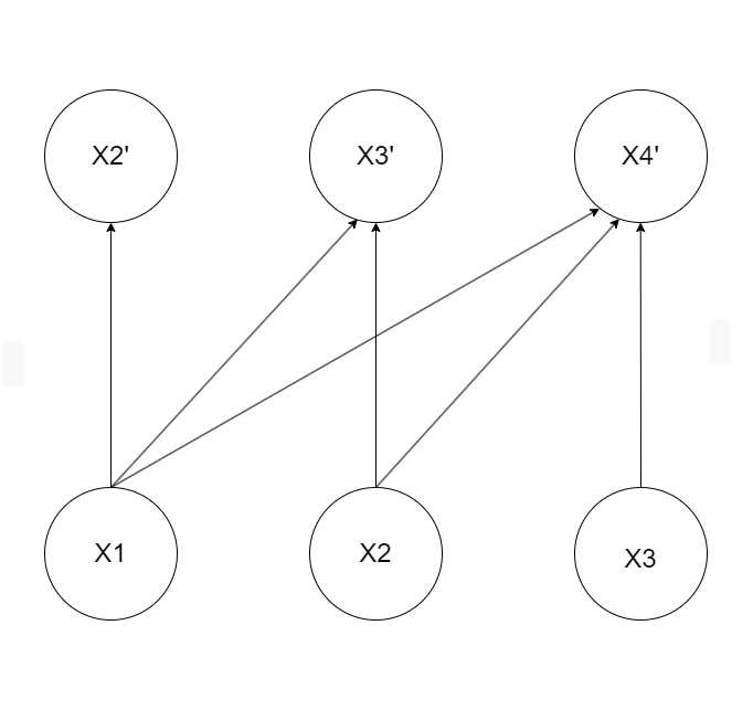
(b) Transformer self-attention flows. The arrows indicate which inputs are received for making each prediction based on a time series $X$.

Figure 5: Insights into the used Transformer architecture.

For every output token, the self-attention score measures the importance of looking at each of the tokens previously seen in the sequence, for predicting the current token. In this traditional attention model (left in Figure 6), the formula to calculate the attention score is provided in Equation 6, and involves computing the dot product between the query vector ($Q$) and the key vector ($K)$ of the current token. For details, the reader is referred to Radford et al. (2018).

$$\textit{Attention(Q, K, V)}=softmax(\frac{QK^{T}}{\sqrt{d_{k}}})V$$ (6)

whereby $\sqrt{d_{k}}$ represents both the dimension of the key vector $K$ as well as the query vector $Q$, and $V$ is the value vector.

4.2 Synthesizer Transformer

Tay et al. (2021)’s Synthesizer Transformer is able to learn attention weights synthetically, without token-token interaction. This increases the speed of the Transformer by up to 60%. Synthesizer Transformers can do this by removing the notion of query-key-values in the self-attention calculation and instead directly synthesizing the attention matrix. This is done using input $X_{h,l}\in\mathbb{R}^{N\times d}$ , where $h$ is the number of heads, $l$ is the sequence length and $d$ is the dimensionality of the model. This eliminates the need to calculate the dot product attention as described in the previous subsection. In their original paper, Tay et al. (2021) propose several synthetic attention variants, in this work, we implemented some of the best performing variants: dense, random, both of their factorized version, as well as a combination of dense and random with the Vanilla Transformer attention.

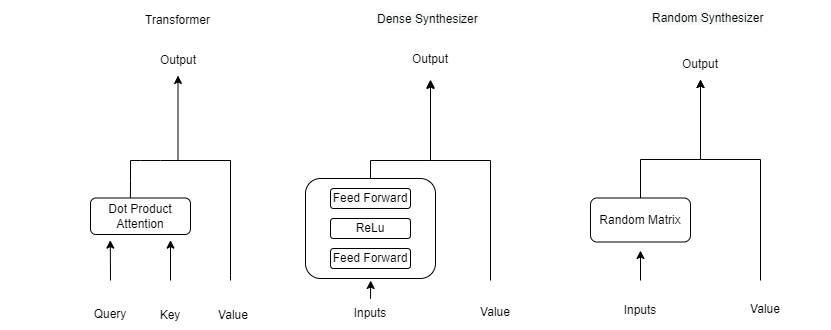
Figure 6: Types of self-attention mechanisms. On the left side, the traditional self-attention mechanism is depicted. The Dense and Random Synthesizer attention mechanism are shown next to it. Figure inspired by Tay et al. (2021).

Dense

This type of dense synthetic attention uses a two-layer feed-forward network with ReLU activation to replace the traditional dot product attention. The attention matrix is simply learned by the dense neural network.

$$\textit{Attention(V)}=Softmax(W_{2}(\sigma_{R}(W_{1}(X_{h,l})))V$$ (7)

whereby $W_{2}$ and $W_{1}$ are feed-forward layers and $\sigma_{R}$ is a ReLu function

Random

The random synthetic attention mechanism does not rely on pairwise token interactions or any information from individual tokens. This way, it aims to capture a global task-specific alignment that obtains good results across a large number of samples. The attention is calculated as follows:

$$\textit{Attention(V)}=Softmax(R)V$$ (8)

whereby $R$ is a randomly initialised $N\times N$ matrix. The weights in this matrix are then optimized during training.

Factorized Dense and Random

The number of parameters added to the network in the above variations is $d\times N$ and $N\times N$ respectively. When the sequence length is large, these synthetic attention models can be slightly harder to train. Hence, we also included factorized variations, which allow the models to perform competitively in practice. In addition, this form of attention also seems to help prevent overfitting. For details on how to calculate attention the reader is referred to Tay et al. (2021).

Mixture dense and random

All of the proposed synthetic attention variants can be mixed in an additive fashion. This results in mixture Synthesizer Transformers (mix). In this work, we experiment by mixing a dense Synthesizer Transformer and a Vanilla Transformer (mix dense) as well as a random Synthesizer and Vanilla Transformer (mix random). The resulting attention is calculated as the sum of the attention calculated by the Vanilla Transformer and the selected Synthesizer Transformer’s attention.

5 Volatility prediction

5.1 Experimental setup

We conduct a thorough experiment to evaluate the performance of the volatility prediction Synthesizer Transformer models (with different attention mechanisms) and compare it to existing baseline models: Vanilla Transformer, LSTM, and GARCH. We first perform hyperparameter optimization using the validation set. The final results using the best parameters are reported on the test set. After finding the best model, we use Captum, a PyTorch library for model interpretability, to identify the input features that contribute most to the prediction result.

We evaluate the models on two tasks: predicting calculated volatility (regression) and predicting volatility spikes (classification). The latter is accomplished by converting the predicted volatility values into two classes: ‘volatility spike’ and ‘non-volatility spike’. A prediction is considered to be a volatility spike when the predicted volatility is greater than or equal to 1 and the log-returns were positive, otherwise we label it as ‘non-volatility spike’.

5.1.1 Training-Test Split

We train our models using the dataset described in Section 3, split into a training, validation, and test set as described below:

• Complete dataset: 02/01/2016 to 21/09/2021 (2,090 days).

• Training set: 02/01/2016 to 02/01/2020 (1,462 days) (70%).

• Validation set: 03/01/2020 to 11/11/2020 (314 days) (15%).

• Test set: 12/11/2020 to 21/09/2021 (314 days) (15%).

There are a total of 232 volatility spikes in the training set and 38 volatility spikes in the validation set. In the test set, there are 46 volatility spikes. We should note that the non-stationarity of financial data is a known issue (De Prado, 2018). Ideally, we would train and test with a rolling time frame over our entire dataset, however, due to the fact that the Transformer model needs as much data as possible, we use an out-of-time test set.

5.1.2 Baseline comparison models

Since we are working with a new dataset, there are no existing benchmarks available to directly compare our results to. In order to overcome this, we trained a few baseline models: a Vanilla Transformer, long-short term memory model (LSTM), and GARCH.

The Vanilla Transformer is the same architecture as our proposed Synthesizer Transformer, but uses the original attention mechanism as per Subsection 4.1. Secondly, long-short term memory models (LSTMs) (Hochreiter and Schmidhuber, 1997) are a type of recurrent neural network that are known for their ability to capture long-term dependencies in time series data as well as avoid the vanishing gradient issue (Chuan and Herremans, 2018). The full configuration of the networks used as baseline is described in Subsection 5.2. Finally, we also explore a statistical model often used in time series analysis: Generalized AutoRegressive Conditional Heteroskedasticity, or GARCH (Li et al., 2002). This model extends the Autoregressive Conditional Heteroskedastic Models (ARCH) model, by including a moving average component (ma) joint with the autoregressive component. This model is often used for volatility prediction, even for Bitcoin  (Dyhrberg, 2016). As our baseline model, we use GARCH(1,1), which is the first order GARCH model using the ARCH library in Python .

5.1.3 Evaluation Metrics

We use several metrics to evaluate the volatility prediction models: root mean square error (RMSE), F1-score, precision, and recall. The first metric looks directly at the regression results, the others look at the resulting predicted volatility spikes (classification). For the regression evaluation, we opted to use RMSE as it is more sensitive to prediction errors with a large difference from the ground truth.

When evaluating volatility spike prediction, we need to take into account that our (test) dataset is not balanced as there are fewer volatility spikes (60) than non-volatility spikes (254). We use precision to see how many correctly predicted spikes (TP) the model predicted correctly out of all predicted spikes (TP+FP).

$$Precision=\frac{TP}{TP+FP}$$ (9)

Recall complements precision by measuring how many spikes the model predicted correctly out of the actual spikes.

$$Recall=\frac{TP}{TP+FN}$$ (10)

In addition, the F1-score provides an integrated metric as the harmonic mean between precision and recall. Overall, a balance of high recall and high precision is preferred because it assumes that the model is well fitted, although it is possible to rely solely on either recall or precision depending on the use case.

$$F1-score=\frac{2*Precision*Recall}{Precision+Recall}=\frac{2*TP}{2*TP+FP+FN}$$ (11)

5.2 Hyperparameter tuning and implementation details

We set the sequence length of all Transformer models to be 64 and the weight decay to be $1\text{e}^{-6}$. We train all the neural network models using Adam optimizer with an initial learning rate of $1\text{e}^{-5}$. All Transformer models use early stopping with the maximum number of epochs set to 10,000 and a patience of 200 to prevent overfitting. In addition, we use the validation set to finetune the models’ hyperparameters as displayed in Table 1. The resulting best parameter settings with the lowest RMSE loss on the validation set are displayed in Table 2.

Feature	LSTM models	Transformer models
Number of layers	1, 2, 4, 8	1, 2, 4, 8
Number of hidden layers	16, 32, 64, 128	NA
Number of heads	NA	2, 4, 8
Batch size	4, 8, 16, 32, 64	4, 8, 16, 32, 64
Dropout	0.1, 0.2	0.1, 0.2

Table 1: An overview of the hyperparameters tested for different neural network architectures.

Model	Best hyperparameter settings
LSTM	batch size=4, dropout=0.2, hidden layer=64, layers=8
Transformer (V)	batch size=4, dropout=0.2, heads=4, layers=2
Synthesizer (R)	batch size=4, dropout=0.2, heads=4, layers=4
Synthesizer (FR)	batch size=4, dropout=0.2, heads=4, layers=8
Synthesizer (D)	batch size=4, dropout=0.2, heads=8, layers=4
Synthesizer (FD)	batch size=4, dropout=0.2, heads=4, layers=4
Synthesizer (MD)	batch size=4, dropout=0.1, heads=2, layers=4
Synthesizer (MR)	batch size=4, dropout=0.1, heads=8, layers=2

Table 2: The best hyperparameters based on the validation set, for the different Transformer models. We use R for random, F for factorised, M for mixed, D for dense, and V for Vanilla models.

5.3 Volatility prediction results

The results for predicting next-day volatility are displayed in Table 3. The left column displays the RMSE for the regression problem (predicting next-day volatility). We then used a threshold $T$, to determine if a volatility spike was predicted. Our default value for $T$ is 1, and for this value we show the F1-score, precision, and recall in the table. We also included the number of True Positives and False Negatives for a few other thresholds to gain insight in how to improve the prediction certainty in Table 4.

From the table, we can see that many of the proposed Synthesizer Transformer models perform well, both in terms of the F1-score (which is consistently above 0.377) as well as RMSE (which is close to 0.1). The baseline LSTM model as well as the Vanilla Transformer consistently perform worse with F1-scores of 0.1714 and 0.2857 respectively. We also ran a basic GARCH(1,1) model which does not perform very well. Since the predictions were too low, no spikes were detected, leaving the precision and recall as zero. We can speculate that GARCH is not the most appropriate model for our task definition. This is in line with the findings of Naimy and Hayek (2018), who find that GARCH is not well suited in a high-volatility context.

When comparing the different types of Synthesizer Transformers, the dense model has a slightly better performance, with the model with factorized dense attention obtaining 0.101 in RMSE and 0.4625 in F1-score. In general, the factorised models slightly outperform the non-factorized models in terms of the F1-score.

Model	RMSE	F1-score	Precision	Recall	TP	FN	TN	FP
GARCH(1,1)	0.303	0.000	0.000	0.000	0	60	254	0
LSTM	0.095	0.171	0.600	0.100	6	54	250	4
Transformer (V)	0.095	0.286	0.500	0.200	12	48	242	12
Synthesizer (R)	0.114	0.374	0.303	0.500	30	30	185	69
Synthesizer (FR)	0.123	0.414	0.316	0.600	36	24	176	78
Synthesizer (D)	0.103	0.448	0.405	0.500	30	30	210	44
Synthesizer (FD)	0.101	0.463	0.370	0.617	37	23	191	63
Synthesizer (MD)	0.100	0.385	0.429	0.350	21	39	226	28
Synthesizer (MR)	0.101	0.400	0.400	0.400	24	36	218	36

Table 3: Model Prediction Results for predicting volatility as regression (RMSE), and as a classification task (F1-score etc.). The True/False Positive/negative (TFPN) results for predicting extreme volatility spikes are also displayed in the last columns. We use R for random, F for factorised, M for mixed, D for dense, and V for Vanilla models.

We included different values for our classification threshold $T$ and reported TP and FN values in Table 4. We see that if we want to have a higher certainty for true positives and a lower chance of false negatives, then setting a higher threshold can help us achieve this. Looking at the Synthesizer (FD), a threshold of 1.2 can help us obtain a recall of 0.85714 (6/(1+6) compared to the original 0.370. This means that we correctly predict 6 our of 7 (larger) volatility spikes. Even with a threshold of 1.1, the Synthesizer Transformer correctly predicts more than 50% of the volatility spikes.

Model TP	FN	TP	FN	TP	FN	TP
	T $\geq$ 1.3		T $\geq$ 1.2		T $\geq$ 1.1
GARCH	0	1	0	7	0	29
LSTM	1	0	2	5	4	25
Transformer (V)	1	0	4	3	6	23
Synthesizer (R)	1	0	5	2	18	11
Synthesizer (FR)	1	0	6	1	21	8
Synthesizer (D)	1	0	6	1	17	12
Synthesizer (FD)	1	0	6	1	21	8
Synthesizer (MD)	1	0	4	3	15	14
Synthesizer (MR)	1	0	4	3	16	13

Table 4: True positive (TP) and false negative (FN) when predicting extreme volatility spikes with different thresholds. We use R for random, F for factorised, M for mixed, D for dense, and V for Vanilla models.

5.4 Model explainability

To gain insight into which features are important for predicting volatility, we used the Captum library for model interpretability. More specifically, we used the feature ablation function (Kokhlikyan et al., 2020) to understand important features that contribute to the prediction of each of the models. Table 5 shows the top 3 features in terms of the absolute value of the weight attribute score based on the feature ablation attribution algorithm for each of the models.

The absolute value of the score, informs us about the importance of this feature for predicting the next-day volatility. Some notable recurring features are important across different models based: taker_buy_volume, HL_spread and volume. Looking back at the initial correlation analysis that we performed in Table LABEL:tab:corr, we confirm the importance of HL_spread and volume for volatility prediction since they have the highest correlation with vol_future.

The feature called taker_buy_volume refers to the volume of perpetual swap trades that market takers buy (and vice versa for taker_sell_volume). Being a ‘taker’ indicates someone who buys or sells at the market price. When the takers’ buy volume is much larger than the takers’ sell volume, this indicates a bullish movement. Other important features include exchange_outflow_mean_ma7 and exchange_transactions_count_inflow. An increase in the latter indicates that more people are active in exchange flows which in turn indicates an increase in interest, leading to an increase in volatility.

Looking at the features that we extracted from Twitter, we find that our variables related to whale transactions also come out as being important with most of them listed as the 10th or 20th most important feature. The most important is the USDminus, which is the 4th most important feature for the Synthesizer Transformer (FD) with an ablation score of -0.0398. This feature is also shown as the 12th most important feature for the Synthesizer Transformer (MD).

Model	Feature 1	Score	Feature 2	Score	Feature 3	Score
V	HL_sprd	0.09	volume	0.07	funding_rates	-0.06
R	taker_sell_volume	0.09	HL_sprd	0.09	taker_buy_volume	0.07
D	exchange_outflow_mean_ma7	-0.07	close	0.05	HL_sprd	0.05
FR	HL_sprd	0.08	taker_buy_volume	0.08	taker_sell_volume	0.08
FD	close	0.07	volume	0.05	exchange_transactions_count_inflow	0.05
MD	taker_buy_volume	0.08	taker_sell_volume	0.06	volume	0.06
MR	volume	0.08	HL_sprd	0.06	taker_buy_volume	0.06

Table 5: The top 3 most important features of the Transformer models according to Captum’s feature ablation function with their attribute score.

6 Trading strategy experiment

In order to evaluate the usefulness of the volatility model, we implemented a few simple trading strategies that take signals from the volatility prediction model, and backtested them. It is worth noting that these strategies are very basic, and can undoubtedly be improved. They solely serve to show whether our predicted volatility metric can help increase our risk-adjusted profits.

6.1 Backtesting strategies

We used the predicted volatility (for each model) and used it as a signal for our strategies. For all of the strategies, we start with an initial capital of $10,000. Each buy signal will be 5% of the remaining capital, with pyramiding. Trading costs were set to 0.1% for this experiment which is relatively higher than many exchanges. The backtesting was performed using the Backtrader library in Python.

We test each of the strategies with and without volatility scaling for setting the position size. As explained above, the strategies typically open a position by buying a fixed percentage of total capital (5%). With volatility scaling, they open a position by buying 5% of capital $times$ volatility. This means that when the volatility is higher, we are trying to gain an edge by using a higher percentage of capital to open a position. Hoyle and Shephard (2018) suggest that volatility scaling can potentially improve the Sharpe ratio of the returns. The four strategies that we tested are described below.

6.1.1 Buy-and-hold

This baseline strategy buys Bitcoin at the start and holds it until the very last day. Due to its constant market exposure, we can expect a higher risk, with, during long enough certain periods, higher returns.

6.1.2 Buy-low-sell-high

An often used strategy is to buy when prices are low, and sell when they are high. We modified this idea to buy when volatility is low ($V<1$) and there is a decrease in log-returns, and sell when a volatility spike is detected ($V\geq 1$), regardless of the price.

6.1.3 Momentum

The proposed Momentum strategy will buy when a volatility spike is predicted and there is an increase in log-returns over the past 2 days. The position will close the next day.

6.1.4 Mean Reversion

The proposed Mean Reversion strategy will buy when a volatility spike is predicted and there is a decrease in the log-returns over the past 2 days. The position will close the next day.

6.2 Evaluation metrics

We used the following metrics to evaluate our backtesting experiment:

Time in market

- The number of days for which a position was open.

Max. Drawdown

- The maximum observed loss from the maximum portfolio value to a subsequent through value before a new maximum is attained (in percentage).

Kelly Criterion

- Determines the optimal theoretical positions size.

Daily VaR(%)

- Daily Value-at-Risk. The VaR reflects the potential loss within a day and a certain confidence level (95%).

PnL

The total profit and loss in percentage.

6.3 Backtesting results

Table LABEL:tab:backtest_results shows the result of our backtesting experiment. The Buy and hold strategy has a Profit and Loss (PnL) of 12.2% for almost one year of holding. The disadvantage of such a strategy, is its constant market exposure, resulting in a high maximum drawdown of 13.66%. Many investors may want to avoid such exposure and instead save fiat for bargain buying opportunities. The buy-low-sell-high strategy performs best in terms of PnL (24%), especially with volatility scaling. This strategy, however, still has a very high time in the market, resulting in a max. drawdown ranging from -15% to -25%. The Momentum strategy, on the other hand, shows a very low time in the market (less than 20%), with a PnL between 2% to 10% for the different proposed Transformer models and a max. drawdown of less than 5%.

In general, profit increases when volatility scaling is used. The Sharpe ratio, Kelly criterion and PnL generally all increase when using volatility scaling for position size, compared to unscaled position sizing. The risk, however, also increases in terms of Daily VaR and max. drawdown. Hence, investors and traders have to weigh the cost and benefits of volatility scaling and see whether are they comfortable adding more risk to their strategy so as to profit more.

	Time In	Sharpe	Max	Kelly	Daily
Model	Market(%)	Ratio	Drawdown(%)	Criterion(%)	VaR(%)	PnL(%)
buy and hold	100	0.8	-13.66	6.84	-1.27	12.2
Transformer (V)
(U) buy-low-sell-high	94.0	0.94	-10.83	8.16	-1.21	14.2
(S) buy-low-sell-high	94.0	0.96	-17.08	8.4	-2.0	24.1
(U) Momentum	2.0	0.84	-0.01	43.76	-0.01	0.148
(S) Momentum	2.0	0.84	-0.03	43.7	-0.03	0.307
(U) Mean Reversion	9.0	-0.14	-2.56	-2.4	-0.31	-0.571
(S) Mean Reversion	9.0	0.03	-5.17	0.55	-0.71	-0.006
Synthesizer Transformer (R)
(U) buy-low-sell-high	75.0	1.06	-7.76	9.37	-1.04	14.1
(S) buy-low-sell-high	75.0	1.0	-12.83	9.0	-1.82	22.9
(U) Momentum	15.0	0.94	-0.93	10.65	-0.21	2.43
(S) Momentum	15.0	1.09	-1.95	12.13	-0.48	6.58
(U) Mean Reversion	23.0	-0.03	-5.77	-0.46	-0.55	-0.395
(S) Mean Reversion	23.0	0.04	-12.92	0.55	-1.31	-0.361
Synthesizer Transformer (FR)
(U) buy-low-sell-high	70.0	0.59	-13.37	5.51	-0.98	6.70
(S) buy-low-sell-high	70.0	0.32	-23.56	3.12	-1.77	5.12
(U) Momentum	17.0	0.05	-3.26	0.72	-0.28	0.135
(S) Momentum	17.0	0.22	-7.07	2.8	-0.64	1.45
(U) Mean Reversion	27.0	0.89	-4.54	9.79	-0.7	7.68
(S) Mean Reversion	27.0	0.84	-11.76	9.44	-1.65	16.8
Synthesizer Transformer (D)
(U) buy-low-sell-high	78.0	0.51	-13.84	4.65	-0.98	5.68
(S) buy-low-sell-high	78.0	0.41	-24.03	3.8	-1.75	7.25
(U) Momentum	10.0	0.81	-1.5	12.13	-0.19	1.88
(S) Momentum	10.0	0.82	-3.11	12.27	-0.39	3.97
(U) Mean Reversion	23.0	0.79	-3.73	9.61	-0.71	6.89
(S) Mean Reversion	23.0	0.75	-8.24	9.22	-1.48	13.2
Synthesizer Transformer (FD) r
(U) buy-low-sell-high	71.0	0.19	-14.59	1.89	-1.01	1.71
(S) buy-low-sell-high	71.0	0.06	-26.18	0.59	-1.88	-0.753
(U) Momentum	13.0	1.54	-1.36	18.78	-0.23	4.55
(S) Momentum	13.0	1.56	-2.64	19.07	-0.47	9.60
(U) Mean Reversion	26.0	1.03	-3.72	11.92	-0.66	8.67
(S) Mean Reversion	26.0	1.03	-8.39	12.13	-1.46	19.2
Synthesizer Transformer (DM)
(U) buy-low-sell-high	85.0	0.76	-16.11	6.86	-1.09	9.96
(S) buy-low-sell-high	85.0	0.77	-25.36	6.95	-1.78	16.21
(U) Momentum	4.0	1.72	-0.02	48.36	-0.14	3.12
(S) Momentum	4.0	1.72	-0.05	48.37	-0.3	6.73
(U) Mean Reversion	16.0	-0.04	-6.99	-0.74	-0.58	-0.483
(S) Mean Reversion	16.0	0.01	-15.37	0.2	-1.32	-0.818
Synthesizer Transformer (MR)
(U) buy-low-sell-high	83.0	0.49	-16.12	4.4	-1.13	6.17
(S) buy-low-sell-high	83.0	0.5	-26.36	4.5	-1.93	10.0
(U) Momentum	6.0	1.97	-0.24	40.56	-0.17	4.32
(S) Momentum	6.0	1.98	-0.5	40.67	-0.35	9.36
(U) Mean Reversion	16.0	0.07	-6.97	1.2	-0.57	0.26
(S) Mean Reversion	16.0	0.16	-15.53	2.95	-1.35	1.62

Table 6: Backtesting Strategy Results. We use U for unscaled (no volatility scaling) position sizing, and S for volatility scaled position sizes.

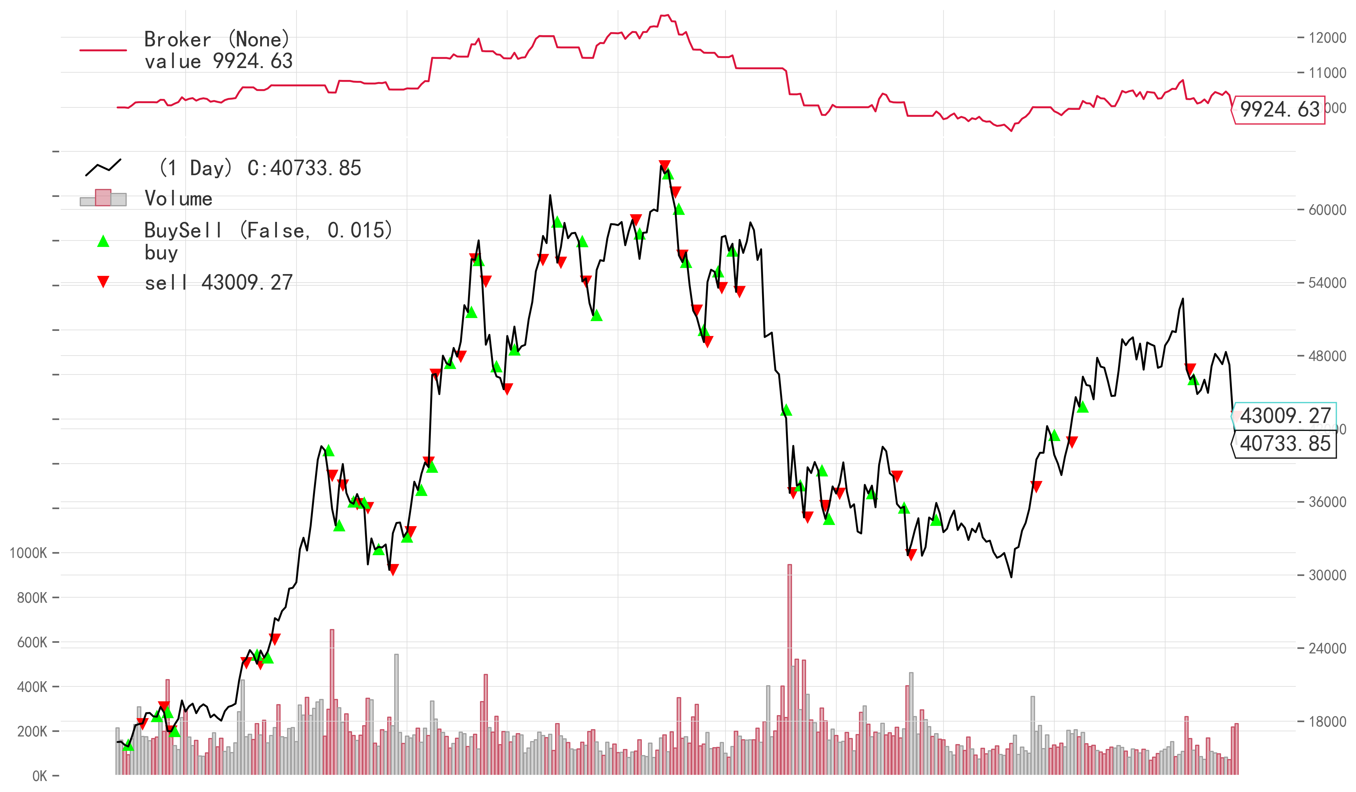
(a) The buy-low-sell-high strategy.

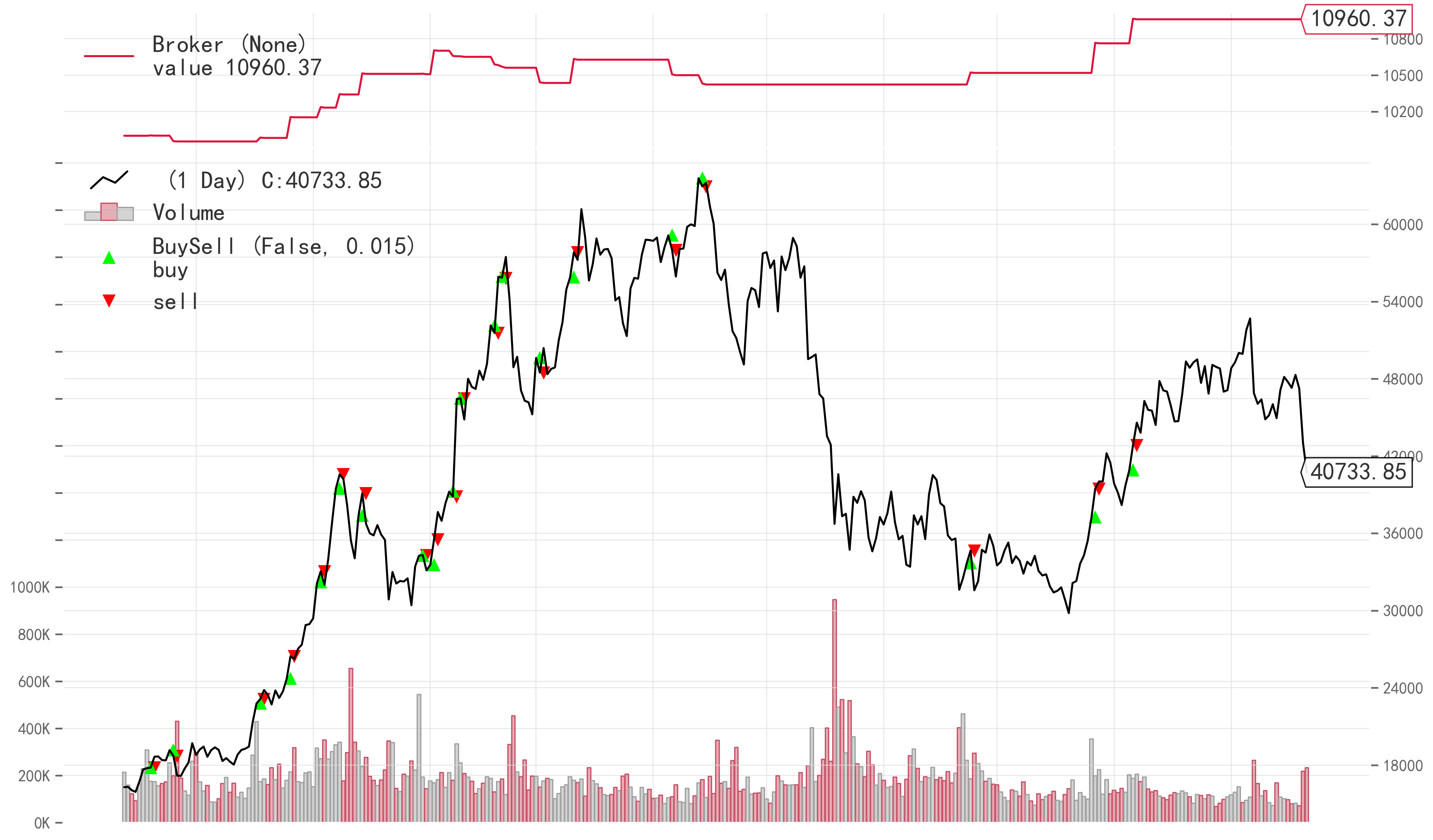
(b) The Momentum strategy.

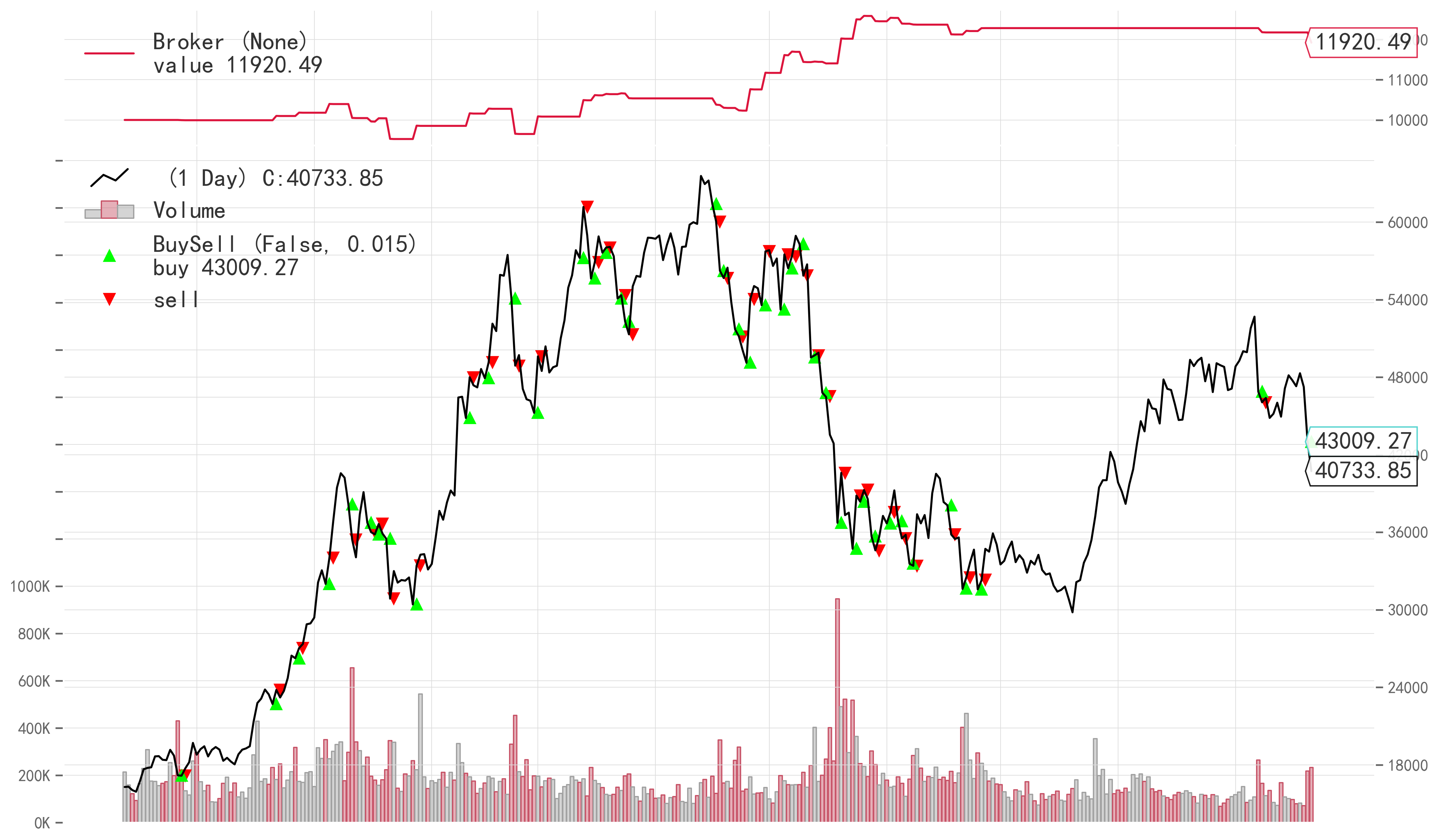
(c) The Mean reversal strategy.

Figure 7: Backtesting graph of the Synthesizer (FD) model. The red down arrows indicate sell signals, and the green up arrows buy signals, and the red curve at the top shows the evolution of the portfolio value.

When looking at one of the better performing models in terms of extreme volatility prediction of the previous section, Synthesizer FD, we notice that the strategies based on this model consistently obtain one of the highest Sharpe ratios. Especially, the momentum and mean reversal strategies (with volatility position scaling), obtain a profit of 9.6% and 19.2%. In Figure 7 details are shown of the actual trades for each of the three (scaled) strategies based on the Synthesizer (FD) model. We notice that the most steady increase in total portfolio value is obtained with both the momentum as well as the mean reversal strategy, which is consistent with the results in table. Overall, while these strategies are overly simple and have ample room for improvements, they show the potential of using volatility predictions for risk reduction and finding trading opportunities.

7 Conclusions

In this work, we investigate the usefulness of CryptoQuant data (e.g. on-chain analytics, exchange data, miner data) as well as whale-alert tweets for predicting Bitcoin’s next-day volatility. The dataset that was analysed in detail, and the correlation between features and next-day volatility was explored. This analysis uncovered the features important for volatility prediction.

We then propose a deep learning Transformer model to predict extreme volatility spikes. In particular, we developed a Synthesizer Transformer, a state-of-the-art architecture that is known for its computational efficiency due to the elimination of the dot-product attention mechanism. After parameter tuning, we performed detailed experiments wherein we examined the influence of different synthetic attention mechanisms on the model’s performance. We also compared the proposed models to baseline models such as LSTM, Vanilla Transformer, and GARCH. The different Synthesizer models outperform all of the baseline models, both in terms of volatility prediction (regression) as well as volatility spike prediction (classification). The proposed Synthesizer Transformer, especially the one with factorised dense attention, manages to obtain state-of-the-art performance when predicting volatility using CryptoQuant data and whale-alert tweets.

To gain insight into the inner workings of our Transformer model, we used the Captum XAI library. This allowed us to uncover important input features such as ‘taker buy volume’ and ‘exchange outflow (ma7)’, and USDminus (USD flowing out of wallets into exchanges, from whale-alert tweets). We thus confirmed the importance of both on-chain and whale-alert Twitter features for volatility prediction.

Finally, we integrated our prediction results with several simple baseline trading strategies. The results show that we are able to minimize drawdown while keeping steady profits. Notably, the Synthesizer Transformer with factorized dense attention performs very well and mitigates downside risk while maintaining a steady profit. We also notice that volatility predicted by our models is especially powerful when used to perform volatility scaling of position sizes, as it increases both the PnL as well as the Sharpe ratio. We should note that these strategies are very simple, each with their own strengths and downfalls, and that they should be improved for use in a real scenario, still, even in this simple form, they demonstrate the power and benefits of our volatility prediction model.

In future research, it would be useful to expand the time frame of both the training and test data, to account for more types of markets. It may also be useful to explore this model for other asset types and on different time scales. Currently, our complete model source code (including trained models) is available online, so that it may be used by anyone interested in forecasting extreme volatility movements in the Bitcoin market.

Appendix A Overview of features

Variable	Description
Inter-entity flow:
etom_flow_total	The total amount of BTC transferred from exchanges to mining pools
etom_transactions_count_flow	Number of transactions from exchanges to mining pools
etom_flow_mean	Mean amount of BTC transferred from exchanges to mining pools
mtoe_flow_total	The total amount of BTC transferred from mining pools to exchanges
mtoe_transactions_count_flow	Number of transactions from mining pool to exchange
mtoe_flow_mean	Mean amount of BTC transferred from mining pools to exchanges
Exchange flows:
exchange_inflow_total	Total amount of BTC flowing into exchanges
exchange_inflow_top10	Total amount of BTC flowing into top 10 exchanges
exchange_inflow_mean	Average daily transaction value for transactions flowing into exchanges
exchange_inflow_mean_ma7	7-day moving average of mean exchange_inflow_mean
exchange_outflow_total	Total amount of BTC flowing out of exchanges
exchange_outflow_top10	Total amount of BTC flowing out of top 10 exchanges
exchange_outflow_mean	Average daily transaction value for transactions flowing out of exchanges
exchange_outflow_mean_ma7	7-day moving average of exchange_outflow_mean_ma7
exchange_addresses_count_inflow	Number of addresses involved in inflow transactions
exchange_addresses_count_outflow	Number of addresses involved in outflow transactions
exchange_transactions_count_inflow	Number of transactions flowing into exchanges
exchange_transactions_count_outflow	Number of transactions flowing out of exchanges
exchange_minus	Net amount of BTC flowing out of exchanges
exchange_plus	Net amount of BTC flowing into exchanges
Miner flows:
miner_inflow_total	Total amount of BTC flowing into mining pool wallets
miner_inflow_top10	Total amount of BTC flowing into top 10 mining pool wallets
miner_inflow_mean	Average daily transaction value for transactions flowing into mining
	pool wallets
miner_inflow_mean_ma7	7-day moving average of miner_inflow_mean
miner_outflow_total	Total amount of BTC flowing out of mining pool wallets
miner_outflow_top10	Total amount of BTC flowing out of top 10 mining pool wallets
miner_outflow_mean	Average daily transaction value for transactions flowing out of mining
	pool wallets
miner_outflow_mean_ma7	7-day moving average of miner_outflow_mean
miner_addresses_count_inflow	Number of addresses involved in inflow transactions
miner_addresses_count_outflow	Number of addresses involved in outflow transactions
miner_transactions_count_inflow	Number of transactions flowing into BTC miner wallets
miner_transactions_count_outflow	Number of transactions flowing out of BTC miner wallets
miner_minus	Net amount of BTC flowing out of miner wallets
miner_plus	Net BTC amount of BTC flowing into miner wallets
Network indicators:
cdd	Coins destroyed by flowing into exchanges
sca	The sum of the days of all coins that was in a kept single wallet
Market data:
open	Opening price of BTC in USD at the beginning of the day
high	Highest daily price of BTC in USD
low	Lowest daily price of BTC in USD
close	the closing price in USD at the end of the day
volume	Daily amount of BTC traded
open_interest	The BTC Perpetual Open Interest from derivative exchanges
market_cap	Total market capitalization of Bitcoin
funding_rates	Periodic payments to traders based on the difference
	between perpetual contract markets and spot prices
taker_buy_volume	Volume of perpetual swap trades bought by takers
taker_sell_volume	Volume of perpetual swap trades sold by takers
taker_buy_ratio	Ratio of taker_buy_volume divided by taker_total_volume
taker_sell_ratio	Ratio of taker_sell_volume divided by taker_total_volume
long_liquidations	Long leveraged positions in BTC that are forced to exit caused by
	price volatility
short_liquidations	Short leveraged positions in BTC that are forced to exit caused by
	price volatility
long_liquidations_usd	Total Amount in USD in long leveraged positions that are forced to exit
	caused by price volatility
short_liquidations_usd	Total Amount in USD in short leveraged positions that are forced to exit
	caused by price volatility
Market indicator:
MVRV (Market-Value-to-Realized-Value)	A ratio of market_cap divided by realized_cap
Flow indicators:
exchange_whale_ratio	Relative size of the top 10 inflows to total inflows of BTC to exchange
fund_flow_ratio	Amount of Bitcoin that exchanges own among the amount of Bitcoin sent
	to the blockchain network
MPI (Miners’ Position Index)	An index to understand miners’ behavior by examining
	the total outflow out of miner wallets
Twitter whale-alerts:
BTCminus	The amount of Bitcoin flowing out of wallets into exchange
BTCplus	Total amount of Bitcoin flowing into wallets from exchanges
USDminus	Total amount in USD flowing out of wallets into exchanges
USDplus	Total amount in USD flowing into wallets from exchanges
Technical indicators:
ema10	10-day exponential moving average
HL_sprd	High-low spread.
CO_sprd	Close-open spread
log_returns	Logarithmic return of Bitcoin

Table 7: Description of (daily) features used in the proposed framework.

Appendix B Correlation of features with volatility

Feature	R2	Pearson	Spearman
exchange_inflow_total	0.125	0.3528	0.287
exchange_outflow_total	0.102	0.3193	0.2744
etom_flow_total	0.0014	0.0377	0.0876
etom_transactions_count_flow	0.006	0.0777	0.1394
etom_flow_mean	0.0003	0.0172	0.0126
mtoe_flow_total	0.0035	0.0592	0.0758
mtoe_transactions_count_flow	0.02	0.1415	0.2341
mtoe_flow_mean	0.0002	0.0152	-0.0961
exchange_addresses_count_inflow	0.0758	0.2752	0.3047
exchange_addresses_count_outflow	0.0491	0.2217	0.2368
exchange_inflow_total	0.1245	0.3528	0.287
exchange_inflow_top10	0.0589	0.2427	0.2425
exchange_inflow_mean	0.0049	0.0702	-0.0047
exchange_inflow_mean_ma7	0.0007	-0.0267	-0.0751
exchange_transactions_count_inflow	0.0802	0.2833	0.3042
exchange_transactions_count_outflow	0.005	0.0711	0.0499
exchange_whale_ratio	0.042	-0.2048	-0.1863
fund_flow_ratio	0.0429	0.2071	0.1871
mpi	0.0227	0.1507	0.1716
miner_addresses_count_inflow	0.0005	-0.0232	0.1058
miner_addresses_count_outflow	0.0006	-0.0249	0.0227
miner_inflow_total	0.0018	-0.0428	-0.026
miner_inflow_top10	0.0	-0.0035	-0.0002
miner_inflow_mean	0.001	-0.0324	-0.0455
miner_inflow_mean_ma7	0.0034	-0.0586	-0.0748
miner_outflow_total	0.0016	-0.0397	-0.0185
miner_outflow_top10	0.0003	-0.0167	-0.0181
miner_outflow_mean	0.0011	-0.0334	-0.0902
miner_outflow_mean_ma7	0.0039	-0.0622	-0.1197
miner_transactions_count_inflow	0.0	0.0041	-0.0325
miner_transactions_count_outflow	0.0007	0.0268	0.013
market_cap	0.0093	0.0966	0.2006
long_liquidations	0.103	0.3209	0.1245
short_liquidations	0.0341	0.1847	0.1193
long_liquidations_usd	0.0537	0.2318	0.1358
short_liquidations_usd	0.0351	0.1874	0.1342
open	0.0108	0.104	0.2085
high	0.0122	0.1104	0.2175
low	0.0083	0.091	0.1962
close	0.0102	0.1008	0.2058
volume	0.1586	0.3982	0.3705
open_interest	0.0023	0.0483	0.0794
mvrv	0.0177	0.1332	0.1661
cdd	0.0222	0.1491	0.1868
sca	0.0012	0.0351	0.0816
funding_rates	0.0052	-0.0724	-0.0057
taker_buy_volume	0.0274	0.1655	0.2336
taker_sell_volume	0.0274	0.1655	0.2352
taker_buy_ratio	0.0	0.0004	-0.0032
taker_sell_ratio	0.0	-0.0004	0.0032
exchange_outflow_total	0.102	0.3193	0.2744
exchange_outflow_top10	0.0538	0.2319	0.2381
exchange_outflow_mean	0.0473	0.2176	0.206
exchange_outflow_mean_ma7	0.0253	0.159	0.1773
HL_sprd	0.3309	0.5752	0.5117
CO_sprd	0.0068	-0.0825	-0.029
log_returns	0.0098	-0.0992	-0.0254
ema10	0.0121	0.1101	0.2123
BTCminus	0.0542	0.2329	0.0649
BTCplus	0.0	0.0058	0.0248
USDminus	0.0151	0.1227	0.0671
USDplus	0.0009	0.0293	0.035
exchange_minus	0.0004	-0.0197	-0.0416
exchange_plus	0.0454	0.213	0.1104
miner_minus	0.0005	-0.0234	-0.0076
miner_plus	0.0009	-0.0304	-0.0292

Table 8: Correlation between volatility and different input features. Values greater than 0.1 are marked in bold.

Appendix C Descriptive statistics of features

Variable	N	Mean	Std	Minimum	Maximum	Skewness	Kurtosis
etom_flow_total	2090	671.64	1782.41	5.31	40381.38	12.24	199.89
etom_transactions_count_flow	2090	324.09	314.13	51.00	5935.00	8.19	101.87
etom_flow_mean	2090	1.81	2.87	0.0769	71.49	17.19	374.87
mtoe_flow_total	2090	924.30	1757.58	90.25	56263.99	19.77	535.17
mtoe_transactions_count_flow	2090	408.73	344.20	46.00	5602.00	6.06	53.43
mtoe_flow_mean	2090	3.27	10.28	0.298	332.92	20.48	562.53
cdd	2090	1.21e+07	1.73e+07	1.33e+06	3.97e+08	9.93	161.97
sca	2090	1.63e+10	3.10e+09	1.14e+10	2.23e+10	0.389	-1.18
open	2090	10961.95	13905.24	359.09	63555.94	2.08	3.48
high	2090	11321.22	14356.97	373.97	64894.67	2.07	3.39
low	2090	10557.51	13376.04	352.40	62016.75	2.10	3.57
close	2090	10981.18	13918.65	358.85	63572.72	2.08	3.46
volume	2090	104172.70	97245.49	3624.27	1.39e+06	3.32	25.21
open_interest	907	3.60e+09	3.53e+09	4.38e+08	1.48e+10	1.21	0.178
market_cap	2090	2.00e+11	2.62e+11	5.41e+09	1.19e+12	2.10	3.50
funding_rates	1956	0.00760	0.0250	-0.257	0.159	0.632	12.90
taker_buy_volume	2090	3.48e+09	5.89e+09	39306.00	4.71e+10	2.51	7.01
taker_sell_volume	2090	3.52e+09	5.98e+09	60220.00	4.83e+10	2.54	7.24
taker_buy_ratio	2090	0.497	0.0384	0.266	0.819	-0.310	11.04
taker_sell_ratio	2090	0.503	0.0384	0.181	0.734	0.310	11.04
long_liquidations	904	4212.18	9965.51	7.86	178839.46	11.47	178.48
short_liquidations	904	2451.05	4980.42	3.47	113129.98	13.28	272.97
long_liquidations_usd	904	7.07e+07	1.43e+08	89528.66	2.03e+09	6.73	66.14
short_liquidations_usd	904	3.89e+07	5.51e+07	35850.00	5.11e+08	3.54	17.95
MVRV(Market-Value-to-Realized-Value)	2090	1.90	0.694	0.695	4.84	0.875	0.387
exchange_whale_ratio	2090	0.410	0.0779	0.101	0.734	0.304	0.716
fund_flow_ratio	2090	0.0669	0.0327	0.000811	0.257	0.748	0.884
MPI(Miners’ Position Index)	2090	0.0906	1.28	-1.79	17.62	2.91	21.27
BTCminus	2090	498.77	2096.25	0.00	50983.00	11.09	199.47
BTCplus	2090	2110.08	8208.79	0.00	150730.00	10.95	152.33
USDminus	2090	9.33e+06	4.52e+07	0.00	1.23e+09	13.05	280.52
USDplus	2090	2.89e+07	1.40e+08	0.00	4.80e+09	21.58	671.08
ema10	2082	10924.28	13792.68	376.82	60859.06	2.08	3.43
HL_sprd	2090	0.0633	0.0491	0.00713	0.717	3.14	21.37
CO_sprd	2090	0.00301	0.0410	-0.392	0.271	-0.147	7.49
log_returns	2090	0.00217	0.0414	-0.493	0.240	-0.843	12.57
vol_future	2090	0.561	0.593	0.000234	8.67	3.34	25.92
miner_inflow_total	2090	6365.36	7371.97	617.31	69414.91	3.56	14.73
miner_inflow_top10	2090	2681.30	1934.40	516.95	23227.61	3.48	19.93
miner_inflow_mean	2090	1.64	0.958	0.103	8.71	2.10	6.54
miner_inflow_mean_ma7	2090	1.65	0.813	0.425	4.84	1.55	2.90
miner_outflow_total	2090	6501.13	8085.25	751.89	87732.70	4.03	21.22
miner_outflow_top10	2090	4329.98	3799.29	719.92	59621.15	4.99	42.45
miner_outflow_mean	2090	6.39	4.66	0.580	79.36	4.27	40.34
miner_outflow_mean_ma7	2090	6.40	3.29	1.07	34.92	2.05	10.91
miner_addresses_count_inflow	2090	5323.60	4411.59	1664.00	34392.00	3.37	11.17
miner_addresses_count_outflow	2090	4556.38	5028.56	672.00	55463.00	3.30	13.13
miner_transactions_count_inflow	2090	3573.62	2035.90	1637.00	21456.00	3.40	15.18
miner_transactions_count_outflow	2090	1075.75	936.26	282.00	8833.00	3.21	13.83
miner_minus	2090	866.67	2881.88	0.00	36966.66	6.75	57.83
miner_plus	2090	730.33	2038.84	0.00	32402.41	7.71	79.15
exchange_inflow_total	2090	53086.70	28663.04	11099.87	338823.11	2.25	11.03
exchange_inflow_top10	2090	20998.42	11238.30	5053.41	134045.94	3.22	19.60
exchange_inflow_mean	2090	1.47	0.72	0.405	7.46	1.89	7.05
exchange_inflow_mean_ma7	2090	1.47	0.602	0.525	4.16	1.16	0.926
exchange_outflow_total	2090	52382.69	27237.06	11922.52	334359.32	2.17	11.36
exchange_outflow_top10	2090	25372.54	12905.31	5475.27	128484.75	2.31	10.34
exchange_outflow_mean	2090	4.94	3.01	0.435	29.57	1.75	5.97
exchange_outflow_mean_ma7	2090	4.93	2.55	1.00	15.79	1.03	0.911
exchange_addresses_count_inflow	2090	48372.63	24352.00	14052.00	234312.00	3.29	17.01
exchange_addresses_count_outflow	2090	43924.36	34987.83	8963.00	397816.00	3.97	23.97
exchange_transactions_count_inflow	2090	39649.27	21199.12	8512.00	216757.00	2.94	15.11
exchange_transactions_count_outflow	2090	12393.55	5948.59	2478.00		2.25	13.26
exchange_minus	2090	2434.06	5150.79	0.00	108428.54	6.72	98.52
exchange_plus	2090	3137.54	6151.34	0.00	89512.88	5.02	44.07

Table 9: Descriptive statistics for the features.

Variable	N	Mean	Std	Minimum	Maximum	Skewness	Kurtosis	TR
etom_flow_total	2090	5.909	0.935	1.67	10.61	0.514	2.26	1
etom_transactions_count_flow	2090	5.61	0.516	3.93	8.69	1.10	3.73	1
etom_flow_mean	2090	0.912	0.421	0.07	4.28	1.44	6.12	5
mtoe_flow_total	2090	6.51	0.703	4.50	10.9	0.528	2.238	1
mtoe_transactions_count_flow	2090	5.84	0.563	3.83	8.63	0.0680	2.50	1
mtoe_flow_mean	2090	1.14	0.572	0.261	5.81	2.31	9.10	5
cdd	2090	15.96	0.751	14.10	19.80	0.719	0.957	1
sca	2090	23.50	0.188	23.16	23.83	0.186	-1.20	1
open	2090	8.55	1.36	5.88	11.06	-0.331	-0.644	1
high	2090	8.58	1.36	5.92	11.08	-0.338	-0.637	1
low	2090	8.51	1.35	5.86	11.04	-0.327	-0.651	1
close	2090	8.55	1.36	5.88	11.06	-0.332	-0.643	1
volume	2090	11.16	0.967	8.20	14.15	-0.482	-0.168	1
open_interest	2090	9.35	10.70	0.00	23.42	0.277	-1.91	1
market_cap	2090	25.11	1.42	22.41	27.80	-0.344	-0.645	1
funding_rates	2090	0.00711	0.0242	-0.260	0.159	0.706	13.8	0
taker_buy_volume	2090	19.61	3.40	10.58	24.60	-0.907	-0.330	1
taker_sell_volume	2090	19.61	3.38	11.00	24.60	-0.886	-0.390	1
taker_buy_ratio	2090	0.497	0.0384	0.266	0.819	-0.310	11.0	0
taker_sell_ratio	2090	0.503	0.0384	0.181	0.734	0.310	11.0	0
long_liquidations	2090	3.24	3.81	0.00	12.09	0.421	-1.64	1
short_liquidations	2090	3.07	3.60	0.00	11.64	0.407	-1.67	1
long_liquidations_usd	2090	7.39	8.52	0.00	21.43	0.312	-1.86	1
short_liquidations_usd	2090	7.23	8.33	0.00	20.05	0.306	-1.87	1
MVRV(Market-Value-to-Realized-Value)	2090	1.36	0.244	0.834	2.20	0.459	-0.153	2
exchange_whale_ratio	2090	0.410	0.0780	0.101	0.734	0.304	0.716	0
fund_flow_ratio	2090	0.0669	0.0327	0.000811	0.257	0.748	0.884	0
MPI(Miners’ Position Index)	2090	0.0906	1.28	-1.79	17.62	2.91	21.3	0
BTCminus	2090	1.18	2.76	0.00	10.84	1.99	2.11	1
BTCplus	2090	2.53	3.81	0.00	11.92	0.906	-1.05	1
USDminus	2090	2.72	6.27	0.00	20.93	1.89	1.63	1
USDplus	2090	5.47	8.11	0.00	22.30	0.830	-1.27	1
ema10	2090	8.54	1.36	5.93	11.02	-0.334	-0.65	0
HL_sprd	2090	0.379	0.0861	0.192	0.895	0.785	1.203	3
CO_sprd	2090	0.00301	0.0410	-0.392	0.271	-0.147	7.49	0
log_returns	2090	0.00217	0.0414	-0.493	0.249	-0.843	12.6	0
vol_future	2090	0.786	0.217	0.124	1.72	-0.00200	-0.0569	4
miner_inflow_total	2090	8.44	0.690	6.43	11.15	1.18	1.79	1
miner_inflow_top10	2090	7.73	0.530	6.25	10.05	0.759	0.882	1
miner_inflow_mean	2090	1.14	0.202	0.469	2.06	0.672	1.20	3
miner_inflow_mean_ma7	2090	1.25	0.294	0.652	2.20	0.786	0.990	2
miner_outflow_total	2090	8.43	0.730	6.62	11.38	1.12	1.51	1
miner_outflow_top10	2090	8.18	0.571	6.58	11.00	0.908	1.35	1
miner_outflow_mean	2090	1.80	0.366	0.834	4.30	0.827	2.50	3
miner_outflow_mean_ma7	2090	1.55	0.195	0..834	4.30	0.0365	0.698	1
miner_addresses_count_inflow	2090	8.42	0.484	7.42	10.45	1.95	4.25	1
miner_addresses_count_outflow	2090	8.13	0.653	6.51	10.92	1.47	2.12	1
miner_transactions_count_inflow	2090	8.09	0.393	7.40	9.97	1.51	2.78	1
miner_transactions_count_outflow	2090	6.76	0.600	5.64	9.09	1.02	0.776	1
miner_minus	2090	2.78	3.36	0.00	10.52	0.543	-1.41	1
miner_plus	2090	3.62	3.29	0.00	10.39	-0.0393	-1.72	1
exchange_inflow_total	2090	10.76	0.493	9.31	12.73	0.00779	0.294	1
exchange_inflow_top10	2090	9.85	0.445	8.53	11.81	0.248	1.08	1
exchange_inflow_mean	2090	1.11	0.169	0.740	1.95	0.665	0.719	3
exchange_inflow_mean_ma7	2090	1.19	0.234	0.725	2.04	0.782	-0.0268	2
exchange_outflow_total	2090	10.75	0.484	9.39	12.72	-0.0628	0.238	1
exchange_outflow_top10	2090	10.03	0.460	8.61	11.76	0.00670	0.539	1
exchange_outflow_mean	2090	1.64	0.321	0.758	3.09	0.400	0.241	3
exchange_outflow_mean_ma7	2090	1.45	0.188	0.100	1.99	0.170	-0.435	1
exchange_addresses_count_inflow	2090	10.70	0.398	9.55	12.36	0.608	1.54	1
exchange_addresses_count_outflow	2090	10.49	0.616	9.10	12.90	0.172	0.579	1
exchange_transactions_count_inflow	2090	10.48	0.461	9.05	12.29	0.0935	0.770	1
exchange_transactions_count_outflow	2090	9.32	0.460	7.82	11.29	-0.319	0.858	1
exchange_minus	2090	3.70	4.05	0.00	11.59	0.260	-1.80	1
exchange_plus	2090	4.31	4.13	0.00	11.40	-0.00799	-1.87	1

Table 10: Descriptive statistics for all variables after postprocessing. The standardization method (TR) used for each value is indicated in the last column with 0: no change - 1: log() - 2: sqrt root - 3: cube root - 4: power of (1/4) - 5: +1 then log().

References

- Aharon et al. (2022) Aharon, D.Y., Demir, E., Lau, C.K.M., Zaremba, A., 2022. Twitter-based uncertainty and cryptocurrency returns. Research in International Business and Finance 59, 101546.
- Akbiyik et al. (2021) Akbiyik, M.E., Erkul, M., Kaempf, K., Vasiliauskaite, V., Antulov-Fantulin, N., 2021. Ask" who", not" what": Bitcoin volatility forecasting with twitter data. arXiv preprint arXiv:2110.14317 .
- Akyildirim et al. (2021) Akyildirim, E., Goncu, A., Sensoy, A., 2021. Prediction of cryptocurrency returns using machine learning. Annals of Operations Research 297, 3–36.
- Alessandretti et al. (2018) Alessandretti, L., ElBahrawy, A., Aiello, L.M., Baronchelli, A., 2018. Anticipating cryptocurrency prices using machine learning. Complexity 2018.
- Bariviera et al. (2017) Bariviera, A.F., Basgall, M.J., Hasperué, W., Naiouf, M., 2017. Some stylized facts of the bitcoin market. Physica A: Statistical Mechanics and its Applications 484, 82–90.
- Bergsli et al. (2022) Bergsli, L.Ø., Lind, A.F., Molnár, P., Polasik, M., 2022. Forecasting volatility of bitcoin. Research in International Business and Finance 59, 101540.
- Biswas and Gupta (2019) Biswas, B., Gupta, R., 2019. Analysis of barriers to implement blockchain in industry and service sectors. Computers & Industrial Engineering 136, 225–241.
- Black et al. (2012) Black, J., Hashimzade, N., Myles, G., 2012. A dictionary of economics. Oxford university press.
- Blau (2017) Blau, B.M., 2017. Price dynamics and speculative trading in bitcoin. Research in International Business and Finance 41, 493–499.
- Bollerslev (1986) Bollerslev, T., 1986. Generalized autoregressive conditional heteroskedasticity. Journal of econometrics 31, 307–327.
- Brandvold et al. (2015) Brandvold, M., Molnár, P., Vagstad, K., Valstad, O.C.A., 2015. Price discovery on bitcoin exchanges. Journal of International Financial Markets, Institutions and Money 36, 18–35.
- Charandabi and Kamyar (2021) Charandabi, S.E., Kamyar, K., 2021. Prediction of cryptocurrency price index using artificial neural networks: a survey of the literature. European Journal of Business and Management Research 6, 17–20.
- Charandabi and Kamyar (2022) Charandabi, S.E., Kamyar, K., 2022. Survey of cryptocurrency volatility prediction literature using artificial neural networks. Business and Economic Research 12.
- Cheah and Fry (2015) Cheah, E.T., Fry, J., 2015. Speculative bubbles in bitcoin markets? an empirical investigation into the fundamental value of bitcoin. Economics letters 130, 32–36.
- Chuan and Herremans (2018) Chuan, C.H., Herremans, D., 2018. Modeling temporal tonal relations in polyphonic music through deep networks with a novel image-based representation, in: Proceedings of the AAAI Conference on Artificial Intelligence.
- Chung et al. (2014) Chung, J., Gulcehre, C., Cho, K., Bengio, Y., 2014. Empirical evaluation of gated recurrent neural networks on sequence modeling. arXiv preprint arXiv:1412.3555 .
- Colon et al. (2021) Colon, F., Kim, C., Kim, H., Kim, W., 2021. The effect of political and economic uncertainty on the cryptocurrency market. Finance Research Letters 39, 101621.
- De Prado (2018) De Prado, M.L., 2018. Advances in financial machine learning. John Wiley & Sons.
- Dimpfl (2017) Dimpfl, T., 2017. Bitcoin market microstructure. Available at SSRN 2949807 .
- Ding et al. (2020) Ding, Q., Wu, S., Sun, H., Guo, J., Guo, J., 2020. Hierarchical multi-scale gaussian transformer for stock movement prediction., in: IJCAI, pp. 4640–4646.
- Ding et al. (2015) Ding, X., Zhang, Y., Liu, T., Duan, J., 2015. Deep learning for event-driven stock prediction, in: Twenty-fourth international joint conference on artificial intelligence.
- Dyhrberg (2016) Dyhrberg, A.H., 2016. Bitcoin, gold and the dollar–a garch volatility analysis. Finance Research Letters 16, 85–92.
- Engle (1982) Engle, R.F., 1982. Autoregressive conditional heteroscedasticity with estimates of the variance of united kingdom inflation. Econometrica: Journal of the econometric society , 987–1007.
- Fang et al. (2019) Fang, L., Bouri, E., Gupta, R., Roubaud, D., 2019. Does global economic uncertainty matter for the volatility and hedging effectiveness of bitcoin? International Review of Financial Analysis 61, 29–36.
- Gkillas et al. (2021) Gkillas, K., Tantoula, M., Tzagarakis, M., 2021. Transaction activity and bitcoin realized volatility. Operations Research Letters 49, 715–719.
- Grinberg (2012) Grinberg, R., 2012. Bitcoin: An innovative alternative digital currency. Hastings Sci. & Tech. LJ 4, 159.
- Hochreiter and Schmidhuber (1997) Hochreiter, S., Schmidhuber, J., 1997. Long short-term memory. Neural computation 9, 1735–1780.
- Hoyle and Shephard (2018) Hoyle, E., Shephard, N., 2018. Volatility scaling’s impact on the sharpe ratio. Available at SSRN 3279787 .
- Hu et al. (2021) Hu, Z., Zhao, Y., Khushi, M., 2021. A survey of forex and stock price prediction using deep learning. Applied System Innovation 4, 9.
- Jagannath et al. (2021) Jagannath, N., Barbulescu, T., Sallam, K.M., Elgendi, I., McGrath, B., Jamalipour, A., Abdel-Basset, M., Munasinghe, K., 2021. An on-chain analysis-based approach to predict ethereum prices. IEEE Access 9, 167972–167989.
- JAIN (2019) JAIN, D., 2019. Cryptocurrency price prediction using transformer: a deep learning architecture. Ph.D. thesis.
- Jiang et al. (2022) Jiang, K., Zeng, L., Song, J., Liu, Y., 2022. Forecasting value-at-risk of cryptocurrencies using the time-varying mixture-accelerating generalized autoregressive score model. Research in International Business and Finance 61, 101634.
- Jiang (2021) Jiang, W., 2021. Applications of deep learning in stock market prediction: recent progress. Expert Systems with Applications 184, 115537.
- Jung and Choi (2021) Jung, G., Choi, S.Y., 2021. Forecasting foreign exchange volatility using deep learning autoencoder-lstm techniques. Complexity 2021.
- Katsiampa (2017) Katsiampa, P., 2017. Volatility estimation for bitcoin: A comparison of garch models. Economics letters 158, 3–6.
- Kharif (2017) Kharif, O., 2017. The bitcoin whales: 1,000 people who own 40 percent of the market. Bloomberg Businessweek 8.
- Khedr et al. (2021) Khedr, A.M., Arif, I., El-Bannany, M., Alhashmi, S.M., Sreedharan, M., 2021. Cryptocurrency price prediction using traditional statistical and machine-learning techniques: A survey. Intelligent Systems in Accounting, Finance and Management 28, 3–34.
- Kim et al. (2022) Kim, G., Shin, D.H., Choi, J.G., Lim, S., 2022. A deep learning-based cryptocurrency price prediction model that uses on-chain data. IEEE Access .
- Klein et al. (2018) Klein, T., Thu, H.P., Walther, T., 2018. Bitcoin is not the new gold–a comparison of volatility, correlation, and portfolio performance. International Review of Financial Analysis 59, 105–116.
- Kokhlikyan et al. (2020) Kokhlikyan, N., Miglani, V., Martin, M., Wang, E., Alsallakh, B., Reynolds, J., Melnikov, A., Kliushkina, N., Araya, C., Yan, S., et al., 2020. Captum: A unified and generic model interpretability library for pytorch. arXiv preprint arXiv:2009.07896 .
- Lamon et al. (2017) Lamon, C., Nielsen, E., Redondo, E., 2017. Cryptocurrency price prediction using news and social media sentiment. SMU Data Sci. Rev 1, 1–22.
- Li et al. (2019) Li, N., Liu, S., Liu, Y., Zhao, S., Liu, M., 2019. Neural speech synthesis with transformer network, in: Proceedings of the AAAI Conference on Artificial Intelligence, pp. 6706–6713.
- Li et al. (2002) Li, W.K., Ling, S., McAleer, M., 2002. Recent theoretical results for time series models with garch errors. Journal of Economic Surveys 16, 245–269.
- Liashenko et al. (2020) Liashenko, O., Kravets, T., Bobro, O., 2020. Fractionally cointegrated vector autoregression model of spread estimation for metals, in: 2020 10th International Conference on Advanced Computer Information Technologies (ACIT), IEEE. pp. 643–646.
- Liu et al. (2019) Liu, J., Lin, H., Liu, X., Xu, B., Ren, Y., Diao, Y., Yang, L., 2019. Transformer-based capsule network for stock movement prediction, in: Proceedings of the First Workshop on Financial Technology and Natural Language Processing, pp. 66–73.
- Makris et al. (2021) Makris, D., Agres, K.R., Herremans, D., 2021. Generating lead sheets with affect: A novel conditional seq2seq framework, in: 2021 International Joint Conference on Neural Networks (IJCNN), IEEE. pp. 1–8.
- Naimy and Hayek (2018) Naimy, V.Y., Hayek, M.R., 2018. Modelling and predicting the bitcoin volatility using garch models. International Journal of Mathematical Modelling and Numerical Optimisation 8, 197–215.
- Nakamoto (2008) Nakamoto, S., 2008. Bitcoin: A peer-to-peer electronic cash system. Decentralized Business Review , 21260.
- Nguyen et al. (2018) Nguyen, T., de Bodisco, C., Thaver, R., 2018. Factors affecting bitcoin price in the cryptocurrency market: An empirical study. International Journal of Business & Economics Perspectives 13.
- Ni et al. (2008) Ni, S.X., Pan, J., Poteshman, A.M., 2008. Volatility information trading in the option market. The Journal of Finance 63, 1059–1091.
- Patel et al. (2020) Patel, M.M., Tanwar, S., Gupta, R., Kumar, N., 2020. A deep learning-based cryptocurrency price prediction scheme for financial institutions. Journal of information security and applications 55, 102583.
- Platanakis and Urquhart (2019) Platanakis, E., Urquhart, A., 2019. Portfolio management with cryptocurrencies: The role of estimation risk. Economics Letters 177, 76–80.
- Radford et al. (2018) Radford, A., Narasimhan, K., Salimans, T., Sutskever, I., et al., 2018. Improving language understanding by generative pre-training .
- Raheman et al. (2021) Raheman, A., Kolonin, A., Goertzel, B., Hegyközi, G., Ansari, I., 2021. Architecture of automated crypto-finance agent, in: 2021 International Symposium on Knowledge, Ontology, and Theory (KNOTH), IEEE. pp. 10–14.
- Ramos-Pérez et al. (2021) Ramos-Pérez, E., Alonso-González, P.J., Núñez-Velázquez, J.J., 2021. Multi-transformer: A new neural network-based architecture for forecasting s&p volatility. Mathematics 9, 1794.
- Saggu (2022) Saggu, A., 2022. The intraday bitcoin response to tether minting and burning events: Asymmetry, investor sentiment, and “whale alerts” on twitter. Finance Research Letters 49, 103096.
- Sapkota (2022) Sapkota, N., 2022. News-based sentiment and bitcoin volatility. International Review of Financial Analysis 82, 102183.
- Scaillet et al. (2020) Scaillet, O., Treccani, A., Trevisan, C., 2020. High-frequency jump analysis of the bitcoin market. Journal of Financial Econometrics 18, 209–232.
- Shen et al. (2019) Shen, D., Urquhart, A., Wang, P., 2019. Does twitter predict bitcoin? Economics Letters 174, 118–122.
- Sridhar and Sanagavarapu (2021) Sridhar, S., Sanagavarapu, S., 2021. Multi-head self-attention transformer for dogecoin price prediction, in: 2021 14th International Conference on Human System Interaction (HSI), IEEE. pp. 1–6.
- Tay et al. (2020) Tay, Y., Bahri, D., Metzler, D., Juan, D., Zhao, Z., Zheng, C., 2020. Synthesizer: Rethinking self-attention in transformer models. arxiv 2020. arXiv preprint arXiv:2005.00743 2.
- Tay et al. (2021) Tay, Y., Bahri, D., Metzler, D., Juan, D.C., Zhao, Z., Zheng, C., 2021. Synthesizer: Rethinking self-attention for transformer models, in: International Conference on Machine Learning, PMLR. pp. 10183–10192.
- Thao et al. (2021) Thao, H.T.P., Balamurali, B., Roig, G., Herremans, D., 2021. Attendaffectnet–emotion prediction of movie viewers using multimodal fusion with self-attention. Sensors 21, 8356.
- Vaswani et al. (2017) Vaswani, A., Shazeer, N., Parmar, N., Uszkoreit, J., Jones, L., Gomez, A.N., Kaiser, Ł., Polosukhin, I., 2017. Attention is all you need. Advances in neural information processing systems 30.
- Vidal and Kristjanpoller (2020) Vidal, A., Kristjanpoller, W., 2020. Gold volatility prediction using a cnn-lstm approach. Expert Systems with Applications 157, 113481.
- Vilasuso (2002) Vilasuso, J., 2002. Forecasting exchange rate volatility. Economics Letters 76, 59–64.
- Wu et al. (2021) Wu, W., Tiwari, A.K., Gozgor, G., Leping, H., 2021. Does economic policy uncertainty affect cryptocurrency markets? evidence from twitter-based uncertainty measures. Research in International Business and Finance 58, 101478.
- Yang et al. (2020) Yang, L., Ng, T.L.J., Smyth, B., Dong, R., 2020. Html: Hierarchical transformer-based multi-task learning for volatility prediction, in: Proceedings of The Web Conference 2020, pp. 441–451.
- Yao et al. (2018) Yao, Y., Yi, J., Zhai, S., Lin, Y., Kim, T., Zhang, G., Lee, L.Y., 2018. Predictive analysis of cryptocurrency price using deep learning. International Journal of Engineering & Technology 7, 258–264.
- Zhang et al. (2022) Zhang, Q., Qin, C., Zhang, Y., Bao, F., Zhang, C., Liu, P., 2022. Transformer-based attention network for stock movement prediction. Expert Systems with Applications 202, 117239.
- Zheng et al. (2021) Zheng, P., Zheng, Z., Wu, J., Dai, H.N., 2021. On-chain and off-chain blockchain data collection, in: Blockchain Intelligence. Springer, pp. 15–39.
- Zou and Herremans (2022) Zou, Y., Herremans, D., 2022. A multimodal model with twitter finbert embeddings for extreme price movement prediction of bitcoin. arXiv preprint arXiv:2206.00648 .