Reads2Vec: Efficient Embedding of Raw High-Throughput Sequencing Reads Data

Abstract

The massive amount of genomic data appearing for SARS-CoV-2 since the beginning of the COVID-19 pandemic has challenged traditional methods for studying its dynamics. As a result, new methods such as Pangolin, which can scale to the millions of samples of SARS-CoV-2 currently available, have appeared. Such a tool is tailored to take as input assembled, aligned and curated full-length sequences, such as those found in the GISAID database. As high-throughput sequencing technologies continue to advance, such assembly, alignment and curation may become a bottleneck, creating a need for methods which can process raw sequencing reads directly.

In this paper, we propose Reads2Vec, an alignment-free embedding approach that can generate a fixed-length feature vector representation directly from the raw sequencing reads without requiring assembly. Furthermore, since such an embedding is a numerical representation, it may be applied to highly optimized classification and clustering algorithms. Experiments on simulated data show that our proposed embedding obtains better classification results and better clustering properties contrary to existing alignment-free baselines. In a study on real data, we show that alignment-free embeddings have better clustering properties than the Pangolin tool and that the spike region of the SARS-CoV-2 genome heavily informs the alignment-free clusterings, which is consistent with current biological knowledge of SARS-CoV-2.

1 Introduction

The first significant worldwide pandemic to arise in the era of widely accessible high-throughput sequencing tools is COVID-19 [S⁺15]. As a result, SARS-CoV-2 has orders of magnitude more sequencing information than any other virus in history. Research efforts to produce publicly available high-quality full-length nucleotide and amino acid (e.g., spike) sequences in user-friendly formats (e.g., FASTA) have been greatly facilitated by global efforts in the collection, assembly, alignment, and curation of high-throughput sequencing data, such as GISAID [GIS22]. There are already more than $13$ million sequences on GISAID. There probably exist even more unassembled or unaligned raw high-throughput sequencing read samples, because it takes time, money, and quality control to publish a sequence on GISAID or such databases for sequences. As nations worldwide continue to spend substantially on sequencing infrastructure to monitor COVID-19 and upcoming pandemics, this sum will only rise [Rep]. It will thus be essential to this monitoring endeavor to have flexible data analysis processes that can swiftly and automatically process large amounts of such data, perhaps in real time. Since genome (or proteome) assembly and alignment tend to be time-consuming activities from a computing viewpoint, such techniques may not have enough time to complete them [SMG⁺11]. Additionally, selecting and parameterizing an assembler often needs some expertise, yet it still produces an inherent bias that we would like to eliminate [GWEJ07].

By the end of 2020, there were close to one million curated full-length sequences accessible on databases such as GISAID [GIS22], which pushed the study of these sequences into the realm of big data to learn anything about the dynamics, diversity, and evolution of this virus. Many conventional approaches for analyzing viruses that rely on building a phylogenetic tree, such as Nextstrain [HMB⁺18], which can only grow to thousands of sequences, were rapidly made ineffective. Even cutting-edge phylogenetic tree construction techniques, such as IQ-TREE 2 [MS⁺20], can only handle tens of thousands of sequences by leveraging parallel processing. The current approaches, which extend to millions of sequences, use classification or clustering in some capacity, either in place of or in addition to phylogenetic reconstruction. One of the primary aspects of (e.g., SARS-CoV-2) sequences that these approaches prefer to categorize or cluster is lineage label (e.g., B.1.1.7 or the Alpha variant). The cutting-edge Pangolin tool classifier was created using a machine learning (ML) framework built on top of some of the most notable phylogenetics research on the lineage dynamics of SARS-CoV-2, such as  [DPMZ⁺21].

GISAID sequence metadata, such as lineage labels, are currently built using the Pangolin tool. There have also been other approaches that are still based on classification and clustering but were created independently of the Pangolin tool and its body of literature, such as  [MMK⁺21, AAK⁺21, AP21, ABC⁺22]. On sets of GISAID sequences with “ground truth” lineage labels — assigned by the cutting-edge Pangolin tool — such techniques have been demonstrated to have high prediction potential. A million [MMK⁺21] or several million sequences [AP21] have already been used to illustrate scalability.

However, only curated full-length nucleotide or amino acid sequences from sources like GISAID have been used for testing and validation. In this study, we investigate how these current tools might be adapted to this environment given that unassembled, unaligned raw high-throughput sequencing reads data will become increasingly prevalent in the future. Modern tools like Pangolin accept full-length SARS-CoV-2 nucleotide sequences as input, making it challenging to adapt directly to the raw high-throughput reads scenario. The $k$-mers-based approaches [AAK⁺21, AP21], however, are alignment-free by nature, allowing their direct application to such unprocessed high-throughput sequencing reads. In this study, we offer Reads2Vec, a unique alignment-free embedding based on the idea of spaced seeds [BSK15].

Our contributions to this paper are as follows:

1. We propose an efficient and alignment-free embedding approach, called Reads2Vec, which can be used as input to any supervised and unsupervised machine learning method.

2. Using a simulated dataset of $\approx$8K high-throughput reads samples of SARS-CoV-2, we show that Reads2Vec outperforms other state-of-the-art alignment-free embedding methods in terms of predictive performance, and that with the Synthetic Minority Oversampling Technique (SMOTE), we can improve the classification performance even more so.

3. Using a real dataset of $\approx$7K high-throughput reads samples of SARS-CoV-2 (PCR tests from nasal swabs), we show that alignment-free embeddings have better clustering properties (in terms of several internal clustering quality metrics) than Pangolin.

4. Using this real dataset, we also show that a disproportionate number of genomic positions in the spike region of the aligned sequences inform the clustering (in terms of information gain), which is consistent with known properties of the SARS-CoV-2 genome [K⁺20].

5. We perform various clustering comparison analyses of the different embeddings, as well as some statistical analyses to understand properties of such representations.

The rest of the paper is organized as follows. Related work may be found in Section 2. All of the techniques we devise and employ for carrying out the classification and clustering experiments, as well as for assessing the outcomes of those techniques, are described in Section 3. The specifics of our classification and clustering studies on synthetic and real data are provided in Section 4. The outcomes of the conducted experiments are discussed in Section  5. The article is concluded in  6, where some potential avenues for future work are also highlighted.

2 Related Work

By applying classification and clustering to protein sequences as in [SRAPK18, ASU⁺21, AAK⁺21, ABC⁺22, TAP21], some effort has been made in recent years to comprehend the behavior of SARS-CoV-2 using machine learning models. Although these studies use $k$-mers to produce fixed length feature embeddings that can be input to machine learning models, it is unclear if these methods would perform as well on the raw sequencing reads samples directly, since they have only been demonstrated on full-length spike or nucleotide sequences. The classification of metagenomic data has been proposed in [WS14, KD15]. It is unknown, though, if such techniques could be used on samples of SARS-CoV-2 reads. Therefore, it is important to explore how well machine learning models can categorize SARS-CoV-2 sequencing read samples. The authors of [GPC16] employ probabilistic sequence signatures to get precise read binning for metagenomic data. Their research intends to separate the read samples into different groups in order to prevent overestimation of $k$-mer frequencies.

In many fields, including graph analytics [ASK⁺21, AAT⁺20], smart grid [AMAK19, AMK⁺19], electromyography [UAK⁺20], clinical data analysis [AZP22], and network security [AAF⁺20], designing fixed length feature embeddings is a popular research area. Another area of study that addresses the issue of sequence classification entails creating a kernel matrix, also known as a Gram matrix, that contains the separation between pairs of sequences [ASK⁺22, ASU⁺21]. When doing sequence classification, kernel-based classifiers like the support vector machine (SVM) may take these kernel matrices as input. Despite having a strong track record for prediction performance, kernel-based approaches have one disadvantage: they have a prohibitive memory cost [ASU⁺21]. Given that a kernel matrix has a dimension of $n\times n$, where $n$ is the number of sequences, it is nearly impossible to keep a kernel matrix in memory when $n$ is a huge number (e.g., one million sequences), as demonstrated in [ASU⁺21].

For classification and clustering problems, a number of machine learning methods based on $k$-mers have been presented in the literature [SRAPK18, QPTZ20, ASU⁺21, AAK⁺21]. There are many classical algorithms for sequence classification [WS14, KD15]. Although these techniques have been shown to be effective in the corresponding research, it is unclear if they can be applied to coronavirus data. The high computational cost of the techniques (due to the large dimensionality of the data) is also a significant issue with all those methods, which might lead to longer runtimes for the underlying classification algorithms.

For machine learning (ML) tasks like classification and clustering, a number of alignment-based [K⁺20, ABC⁺22], alignment-free [AP21], embedding techniques have recently been presented. One-Hot-Encoding (OHE), a simple method, was employed by the authors in [K⁺20] to create a numerical representation for biological sequences. However, the technique is not scalable because of the enormous dimensionality of the feature vector. Position weight matrix (PWM)-based techniques are used by the authors in [ABC⁺22] to produce feature embeddings for spike sequences. However, it only works for aligned sequences, though, which is a drawback. Making use of phylogenetic applications of $k$-mers counts were initially investigated in [Bla86] where authors suggested the creation of precise phylogenetic trees from several coding and non-coding DNA sequences. The $k$-mers method was used for a description of sequence analysis in metagenomics. An alignment-free SARS-CoV-2 classification method based on $k$-mers, was proposed in [AP21].

3 Methods

Here, we outline all of the methods (designed, and) used in this paper. We first discuss the different embedding methods we use to generate a feature vector representation, including our newly proposed Reads2Vec. We also detail the SMOTE method, for overcoming the class imbalance issue in classification. We then discuss the clustering algorithms we used in this paper, including the Pangolin tool as a baseline for comparison. We then discuss different internal clustering evaluation metrics that we use to measure the performance of the clustering algorithms. Finally, we detail several clustering comparison measures, such as the adjusted Rand index, that we use to compare each pair of clusterings.

3.1 Embedding Approaches

In this section, we describe all embedding approaches we used for the experiments. Figure 4 depicts a flow chart of the three alignment-free embeddings used.

3.1.1 One-Hot Embedding (OHE) [K⁺20]

As a baseline embedding, we use the one-hot encoding (OHE) [K⁺20]. This approach generates a binary vector for each nucleotide $\{A,C,G,T\}$ of a nucleotide sequence, where the vector associated with nucleotide $N$ will have 1s for the positions in this sequence that correspond to $N$, and all other positions will have value $0$. Such binary vectors are generated for all nucleotides and are concatenated to form a single vector.

3.1.2 Spike2Vec [AP21]

Spike2Vec [AP21] is an alignment-free $k$-mers based approach which computes $k$-mers directly from the reads sample. The $k$-mers are sub-strings of length $k$ extracted from the reads using a sliding window, as shown in Figure 1(a). The $k$-mers allow preserving some of the sequential ordering information on the nucleotides within each read. From a read of length $N$ we extract $N-k+1$ $k$-mers.

These generated $k$-mers are then used to create a fixed-length feature vector by taking the frequency of each $k$-mer. The length of this feature vector is $|\Sigma|^{k}$ where $\Sigma$ is the character alphabet (and $k$ is the length of the $k$-mers). In our experiments we took $k=3$ and the alphabet is the nucleotides $\{A,C,G,T\}$. Therefore the feature vector length is $4^{3}=64$.

3.1.3 Minimizers2Vec

We describe a minimizers based embedding, which we name Minimizers2Vec. A minimizer [RHH⁺04] is the lexicographically smallest $m$-mer in forward and reverse order within a window of size $k$.

Minimizers2Vec on Real Short Read Sequences.

Here we just compute the minimizer of each short read (the window is the read), as shown in Figure 1(b), allowing for a much more compact frequency vector, as compared to computing all the $k$-mers.

These generated minimizers are then used to create a fixed-length feature vector in the same way as in the $k$-mers based embedding. Clearly, this approach discards almost entirely the sequences, since it preserves only a representative $m$-mer for each short read.

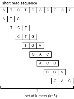
(a) $k$-mers for read “ATCTGACGAC”

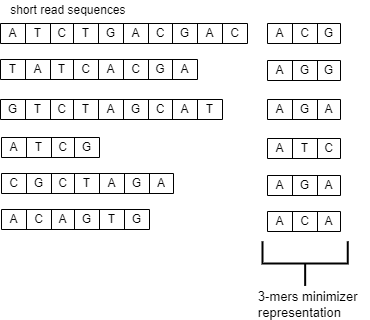
(b) Set of minimizers for a reads sample

Figure 1: Example of $k$-mers, and minimizers. This way of computing minimizer is used on real data only — where we have 1 minimizer per short read.

Minimizers2Vec on Simulated Sequences.

We compute the minimizer of each $k$-mer (the window is the $k$-mer of length 9), as shown in Figure 2, allowing for a much more compact frequency vector, as compared to storing all $k$-mers.

These generated minimizers are then used to create a fixed-length feature vector in the same way as in the $k$-mers based embedding. Clearly, this approach is more compact since it preserves only a representative $m$-mer ($m=3$) for each $k$-mer ($k=9$) in the short read sequence.

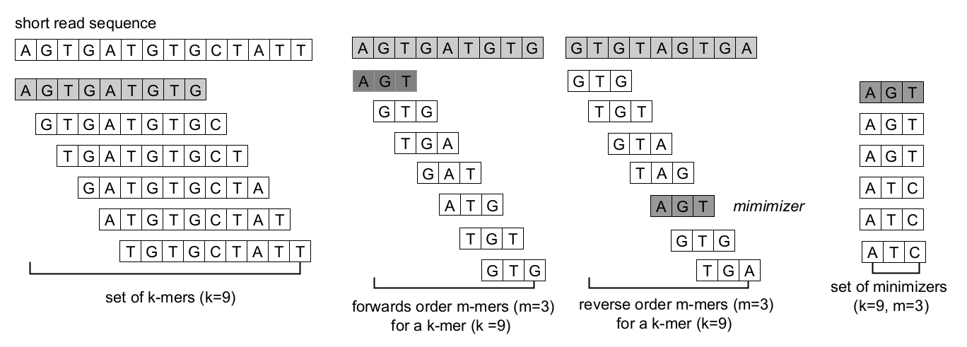
Figure 2: Example for minimizers generation from a short read “ATCTGACGAC” (used to generate Minimizers2Vec for simulated data).

3.1.4 Reads2Vec

Feature vectors for sequences based on $k$-mers frequencies are very large-sized and sparse, and their size and sparsity negatively impact the sequence classification performance. Spaced $k$-mers [SS⁺17] (or spaced seeds [BSK15]) introduced the concept of using non-contiguous length $k$ sub-sequences ($g$-mers) for generating compact feature vectors with reduced sparsity and size. Given a spike sequence as input, it first computes $g$-mers. From those $g$-mers, we compute $k$-mers, where $k<g$. We used $k=4$ and $g=9$ to perform the experiments (see an example in Figure 3). The size of the gap is determined by $g-k$. This method still goes through computationally expensive operation of bin searching, however.

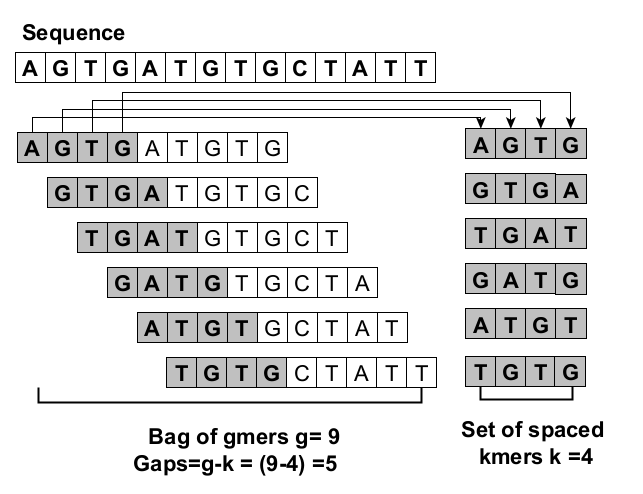
Figure 3: Example for set of spaced $k$-mers for a reads sample (Read2Vec)

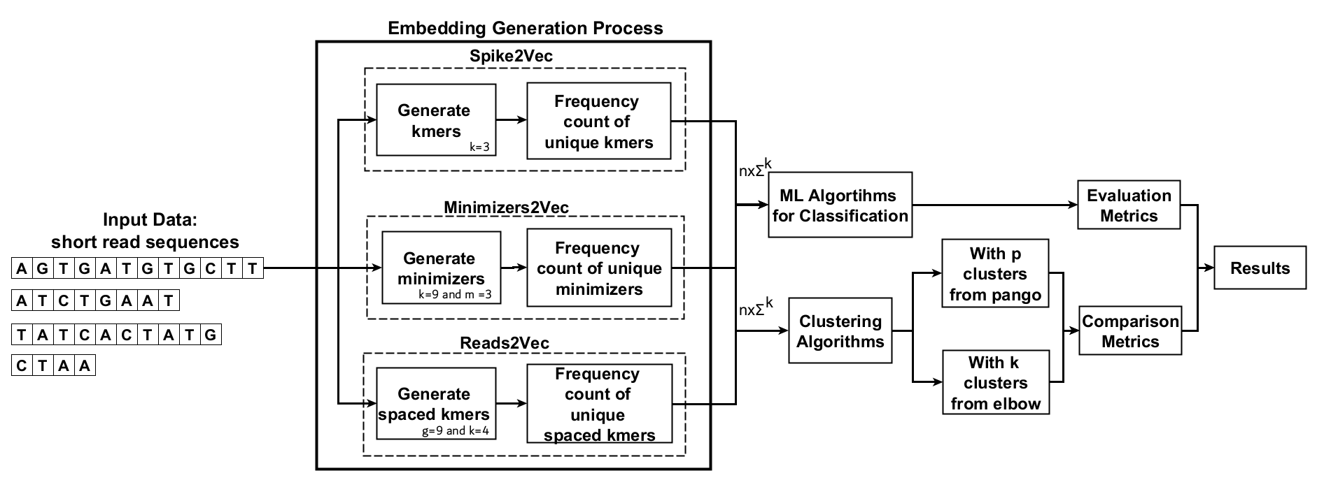
Figure 4: Flow chart of embedding generation and experiments for the three alignment-free embeddings.

3.2 Synthetic Minority Oversampling Technique (SMOTE)

In machine learning based classification, data imbalance is a regular occurrence. Minority samples are significantly smaller in the unbalanced data classification than majority samples, making it challenging for classifiers to learn the minority set. By synthesizing the minority samples or removing the majority samples, one can increase the sensitivity of the minority at the data level. Classifiers are more sensitive to minority labels when using the synthetic minority oversampling method (SMOTE), which synthesizes minority samples without repetition. Minority samples are randomly oversampled, which creates equilibrium between the different classes of samples [MES16]. Random synthesis minority samples, on the other hand, may result in overfitting issues with classification algorithms [YKZZ17]. The blindness of random oversampling is addressed by the synthetic minority oversampling method (SMOTE) [CBHK02]. By randomly picking a minority sample and linearly interpolating between its neighbor samples, SMOTE creates non repetitive minority samples. For unbalanced classification by re-sampling [LJL⁺20], the Synthetic Minority Oversampling Technique (SMOTE) has come to be considered the de facto standard. By using interpolation, SMOTE creates new minority class instances in the areas surrounding the original ones.

3.3 Clustering Algorithms

Each of the feature embeddings of the previous section can be given as input to any of the clustering algorithms that we specify next.

3.3.1 $k$-means [Llo82].

The classical $k$-means clustering method [Llo82] clusters objects based the Euclidean mean.

In order to obtain the optimal number of clusters for $k$-means (and $k$-modes, below), we have used the Elbow method [SAIR11], which makes use of the knee point detection algorithm (KPDA) [SAIR11], as depicted in Figure 5. From this figure, it is clear that $5$ is the optimal number of clusters.

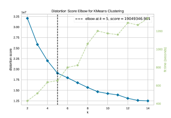
Figure 5: Use of the elbow method for determining the optimal number of clusters in the real data containing 6812 sequences.

3.3.2 $k$-modes [Hua98].

We also cluster with $k$-modes, which is a variant of $k$-means using modes instead of means. Here, pairs of objects are subject to a dissimilarity measure (e.g., Hamming distance) rather than the Euclidean mean. We have used the same value of $k$ as for $k$-means.

3.3.3 Pangolin [Pan]

We also use the Pangolin tool, which takes directly as input the consensus sequence of a sample of reads (see Section 4.1.1), as a baseline for comparison. The Pangolin tool assigns the most likely lineage [OSU⁺21] (called the Pango lineage) to a SARS-CoV-2 genome sequence. The Pangolin dynamic nomenclature [RHO⁺20] was devised for identifying SARS-CoV-2 genetic lineages of epidemiological significance and is used by researchers and public health authorities throughout the world to track SARS-CoV-2 transmission and dissemination.

3.4 Clustering Evaluation Metrics

In this section, we describe the internal clustering evaluation measures used to assess the quality of clustering.

3.4.1 Silhouette Coefficient [Rou87].

Given a feature vector, the silhouette coefficient computes how similar the feature vector is to its own cluster (cohesion) compared to other clusters (separation) [P⁺11]. Its score ranges between $[-1,1]$, where $1$ means the best possible clustering and $-1$ means the worst possible clustering.

3.4.2 Calinski-Harabasz Score [CH74].

The Calinski-Harabasz score evaluates the validity of a clustering based on the within-cluster and between-clusters dispersion of each object with respect to each cluster (based on sum of squared distances) [P⁺11]. There is no defined range for this metric. A higher score denotes better defined clusters.

3.4.3 Davies-Bouldin Score [DB79].

Given a feature vector, the Davies-Bouldin score computes the ratio of within-cluster to between-cluster distances [P⁺11]. There is no defined range for this metric. A smaller score denotes groups are well separated, and the clustering results are better.

3.5 Clustering Comparison Metrics

To compare different clustering approaches, we use the following metrics:

3.5.1 Adjusted Rand Index [HA85].

Given two clusterings, the adjusted Rand index (ARI) computes the similarity between them by considering all pairs of clusters output and counts the pairs that are assigned to the same or different clusters. The value ranges between $0$ and $1$, where $1$ denotes an identical labeling, and approaches 0 as they become more different. A pair of random labelings has an expected ARI of almost 0.

3.5.2 Fowlkes-Mallows Index [FM83].

Given two clusterings, the Fowlkes-Mallows index (FMI) first computes the confusion matrix for the clustering output. The FMI is then defined by the geometric mean of the precision and the recall. Its value range from 0 to 1 with larger value indicating a greater similarity between the clusters.

3.5.3 Completeness Score [RH07].

Given two clustering outputs, the completeness score (CS) evaluates how much similar samples are placed in the same cluster. Its value ranges between $[0,1]$, where $1$ means complete clustering agreement and approaches 0 the further it deviates from this.

3.5.4 V-measure [RH07].

Given two clustering outputs, we first compute homogeneity (evaluate if objects belong to the same or different cluster) and completeness (evaluate how much similar samples are placed together by the clustering algorithm). The V-measure is then defined by the harmonic mean of homogeneity and completeness. This score is a number between $[0,1]$ where $1$ indicates a perfect matching and approaches 0 the further it deviates from this.

4 Experimental Evaluation

In this section, for each of the simulated and real datasets used, we describe how such dataset was collected, and then provide some statistics and visualization of the dataset. We then describe the experimental setup for performing the classification and clustering on the respective datasets.

4.1 Experiments on Simulated Data

In this section, we first give the technical details on how the data were simulated, and then we give some statistics and visualization of this data, as well as mention the classifiers and metrics we used to assess the performance in the results section.

4.1.1 Obtaining the Dataset

We obtained a random sample of 10,181 full-length nucleotide sequences from the $\approx$4 million available on the GISAID [GIS22] database at the time. Each sequence is annotated with a SARS-CoV-2 lineage. Of these, we kept only those sequences whose label appears ten or more times in the set, retaining 8140 (of the 10,181) sequences (see Table 1). From each such sequence, we then simulated a set of short reads using InSilicoSeq [GHE18] with default parameters other than using the MiSeq error model. We implemented these steps in a Snakemake [M⁺21] pipeline, which is available online for reproducibility. The lineage which labels each sequence provides a ground truth label for the corresponding set of short reads simulated from the sequence.

4.1.2 Dataset Statistics

Table 1 provides the statistics about the dataset comprising simulated sets of reads. Note that we combined similar lineages with each other to reduce the class imbalance, e.g., all Delta lineages including B.1.617.2 along with lineages starting with AY are combined to make a single class label “Delta”. In the same manner, the Gamma, Epsilon, and Beta lineages are combined with all of their descendant lineages to make single labels, namely “Gamma”, ”Epsilon”, and “Beta”, respectively. Note that the “Name” column contains the class label, which we are using for the supervised machine learning task, i.e., classification.

Lineage	Region	Name	No. of Sequences
B.1.617.2 and AY lineages	India	Delta	4699
B.1.1.7	UK	Alpha	2587
B.1.177	Spain	Spanish	395
P.1 and descendant lineages	Brazil	Gamma	231
B.1.427 and B.1.429	USA	Epsilon	116
B.1.351 and descendant lineages	South Africa	Beta	65
B.1.621	USA	Mu	19
B.1.525	Canada	Eta	16
B.1.617.1	India	Kappa	12
Total	-	-	8140

Table 1: Variants distribution for a total of 8140 simulated sets of reads. Note that closely-related lineages (with the same name, e.g., Delta) have been merged.

4.1.3 Data Visualization

The t-distributed Stochastic Neighbor Embedding (t-SNE) plots for simulated data without and with SMOTE are shown in Figure 6 and 7, respectively. In Figure 6, we can observe that most of the lineages, including Alpha, Delta, Epsilon, and Gamma are clearly grouped together for all embedding generation methods. An interesting observation here is that in case of Reads2Vec, we can see that Alpha lineage is more clearly separated from the Delta lineage as compared to Minimizers2Vec and Spike2Vec, making it superior in terms of preserving distance between sequences in the original data. In Figure 7, we can observe that although SMOTE introduces more data, most of the lineages are clearly separated from each other in case of Spike2Vec and Reads2Vec. In case of Minimizers2Vec, we can observe that Kappa lineage is separated into two different groups, which is not the case with Spike2Vec and Reads2Vec.

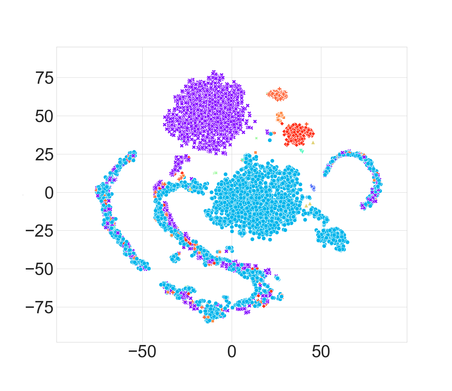
(a) Spike2Vec

(b) Minimizers2Vec

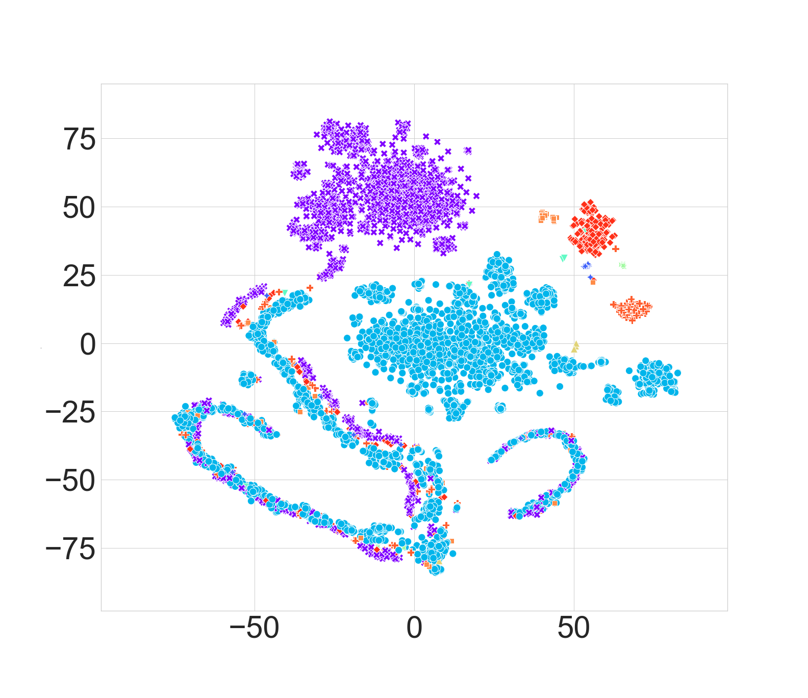
(c) Reads2Vec

Figure 6: t-SNE plots for different embedding methods. This figure is best seen in color.

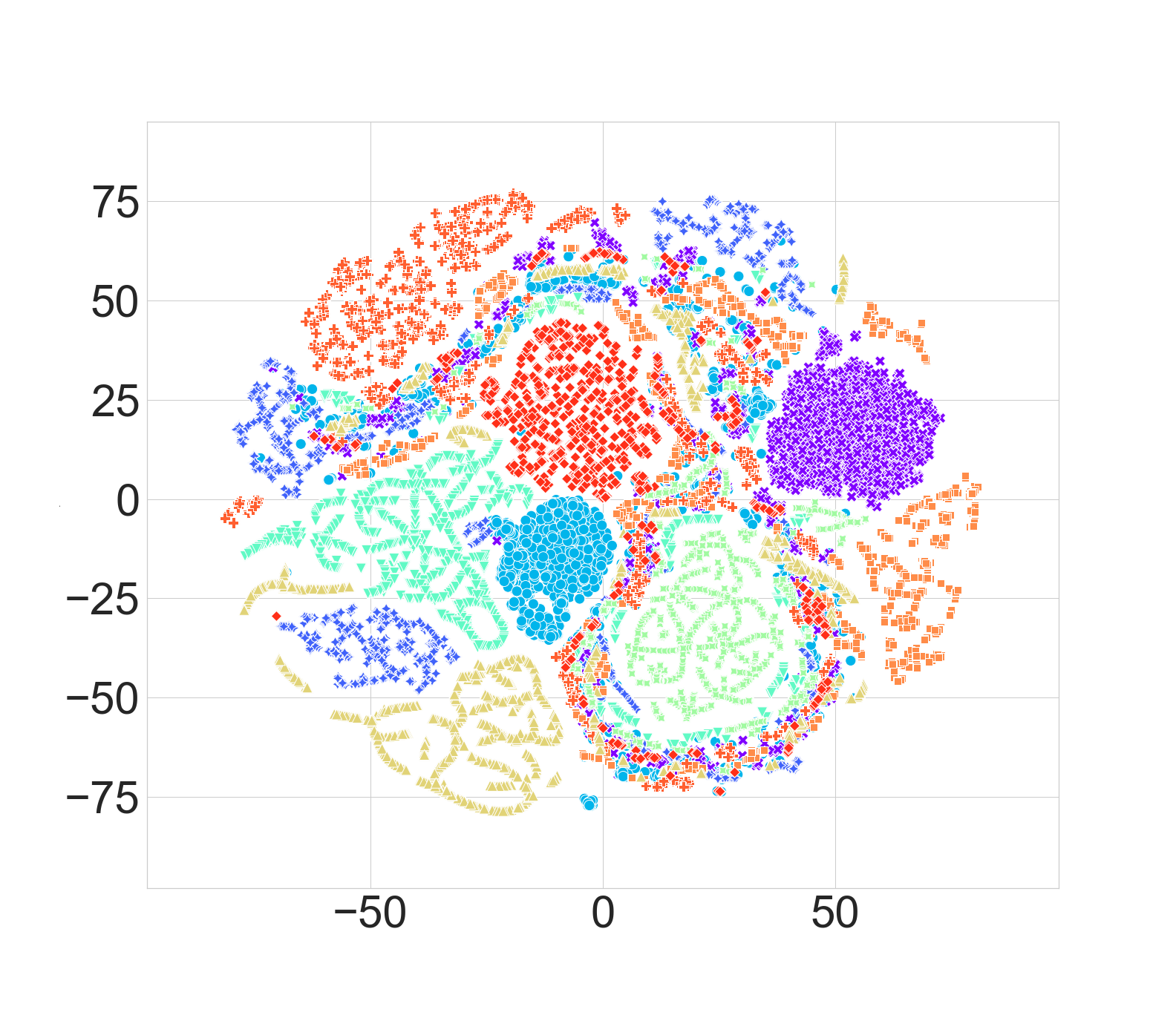
(a) Spike2Vec

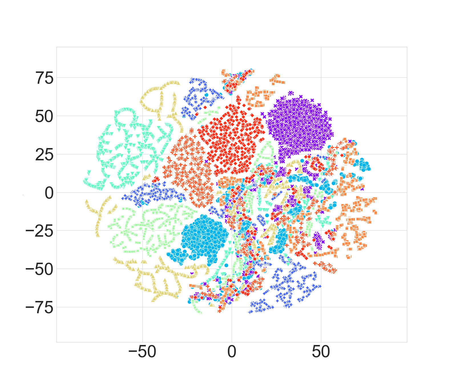
(b) Minimizers2Vec

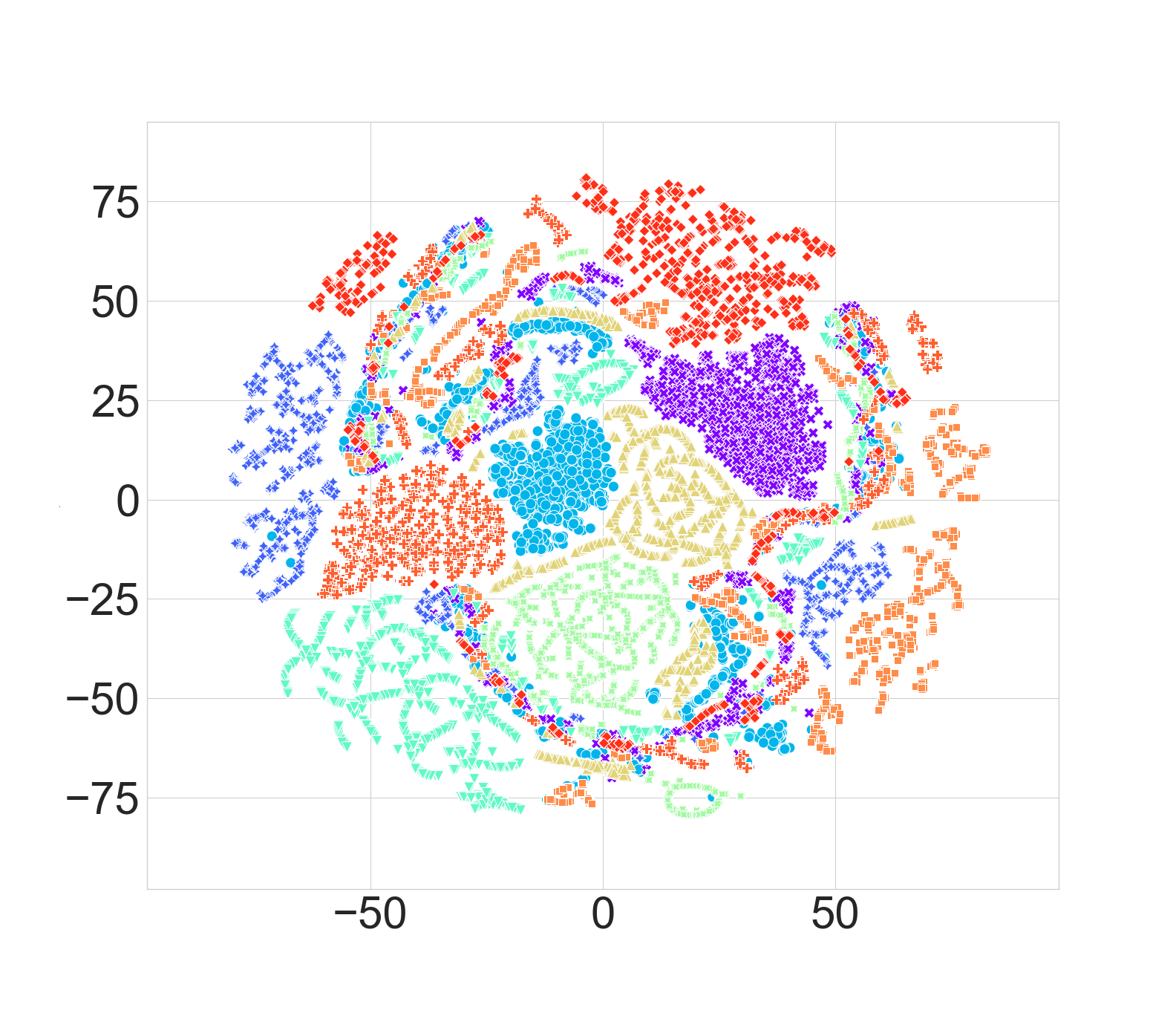
(c) Reads2Vec

Figure 7: t-SNE plots for different embedding methods after SMOTE. This figure is best seen in color.

4.1.4 Evaluation Metrics And Classifiers

Support vector machine (SVM), naive Bayes (NB), multi-layer perceptron (MLP), $k$-nearest neighbors (KNN), random forest (RF), logistic regression (LR), and decision tree (DT) classifiers are used as baseline models for sequence classification. The performance of various models are evaluated using average accuracy, precision, recall, F1 (weighted), F1 (macro), receiver operator characteristic curve (ROC), area under the curve (AUC), and training runtime metrics. Furthermore, the one-vs-rest approach is used to convert the binary evaluation metrics to multi-class ones.

4.2 Experiments on Real Data

In this section, we first give the technical details on how the data were collected and annotated, and then we give some statistics and visualization of this data.

4.2.1 Obtaining the Dataset

We downloaded $6812$ raw high-throughput reads samples of COVID-19 patient nasal swab PCR tests from the NCBI SARS-CoV-2 SRA runs resource (see Section 4.2.2 for some basic descriptive statistics on these data). We then obtained the reference genome from Ensembl, and aligned each sample to this reference genome, called the variants in this sample with respect to the reference genome, and then inserted these variants into the reference genome to generate a consensus sequence. The basic steps in more detail are depicted in Figure 8. We implemented these steps in a Snakemake [M⁺21] pipeline, which is available online for reproducibility. Since these sets of short reads have no ground truth lineage information, we needed to produce a consensus sequence from each such set, in order annotate it with a lineage label using the state-of-the-art Pangolin tool. Note that the one-hot embedding (OHE), e.g., Figure 10(a), is also computed on such a consensus sequence, while the alignment-free Spike2Vec and Minimizers2Vec embeddings are computed directly from the raw reads.

Figure 8: Pipeline for producing consensus sequences. (1) We download the reads samples using the NCBI command line batch Entrez tool fasterq-dump (https://rnnh.github.io/bioinfo-notebook/docs/fasterq-dump.html), and we download the SARS-CoV-2 reference genome (Wuhan-Hu-1) GCA_009858895.3.fasta. (2) Each sample is aligned to this reference genome using bwa mem [Li13] and then compressed to BAM (https://samtools.github.io/hts-specs/SAMv1.pdf) format using samtools [DBL⁺]. (3) From the sample, an “mpileup” is generated with bcftools mpileup [DBL⁺], variants are then called with bcftools call, and the resulting VCF (https://samtools.github.io/hts-specs/VCFv4.2.pdf) file is normalized with bcftools norm. (4) Finally, the consensus FASTA sequence is generated by inserting into the reference genome the variants from the VCF file generated in the previous step, with bcftools consensus.

4.2.2 Dataset Statistics and Visualization

The dataset statistics (the labels are assigned to the samples using the Pangolin tool) for our experiments on raw high-throughput reads samples are given in Figure 9 and Table 2. Both the dataset and the code used in this paper are available online.

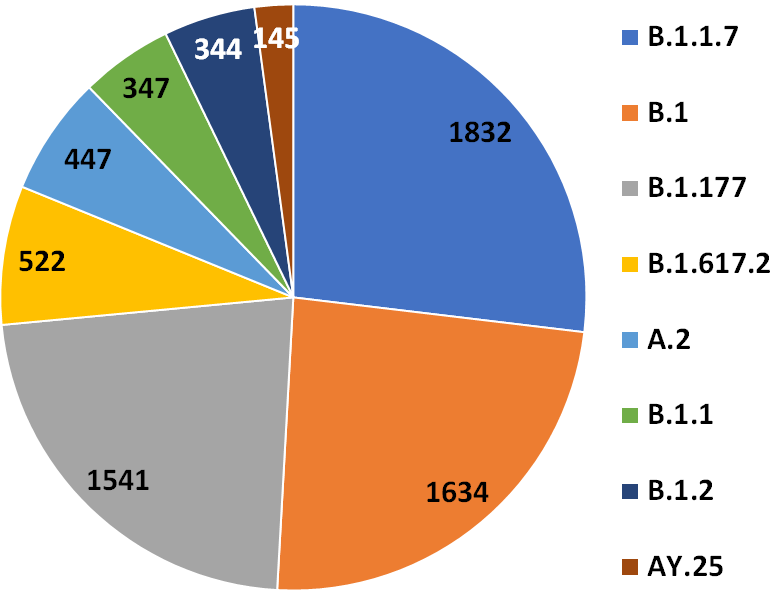
Figure 9: Lineage distribution for the 6812 sets of short reads obtained from NCBI, according to the annotation by Pangolin.

Lineage	Region	Name	No. of Sequences
B.1.1.7	UK	Alpha	1832
B.1	_	_	1634
B.1.177	_	_	1541
B.1.617.2	India	Delta	522
A.2	_	_	447
B.1.1	_	_	347
B.1.2	_	_	344
AY.25	India	Delta	145

Table 2: Lineage distribution for the 6812 sets of short reads obtained from NCBI, according to the annotation by Pangolin, in tabular form.

A first analysis is to check if there is any natural clustering or hidden pattern in the data. However, it is very difficult to visually analyze the information in higher dimensions (i.e., dimensions $>2$). For this purpose, we mapped the data to 2-dimensional real vectors using the t-distributed stochastic neighbor embedding (t-SNE) approach [VdMH08]. The t-SNE plots for different embedding methods are given in Figure 10. For OHE (Figure 10(a)), we can observe that some data is separated into different clusters, such as in the case of lineages A2 and B.1.1.7. For the t-SNE plots of Spike2Vec and Minimizers2Vec embeddings (Figure 10(b) and 10(c) respectively), since we are computing the feature embedding directly from the raw reads sample data, we can observe the difference in the structure of data as compared to OHE. Although there is some overlapping between different lineages, we can still observe some separation between a few lineages, such as B.1.1.7 and B.1.617.2. Since there is no clear separation between different lineages in any of the t-SNE plots (apart from some small groups), clustering this dataset is not easy.

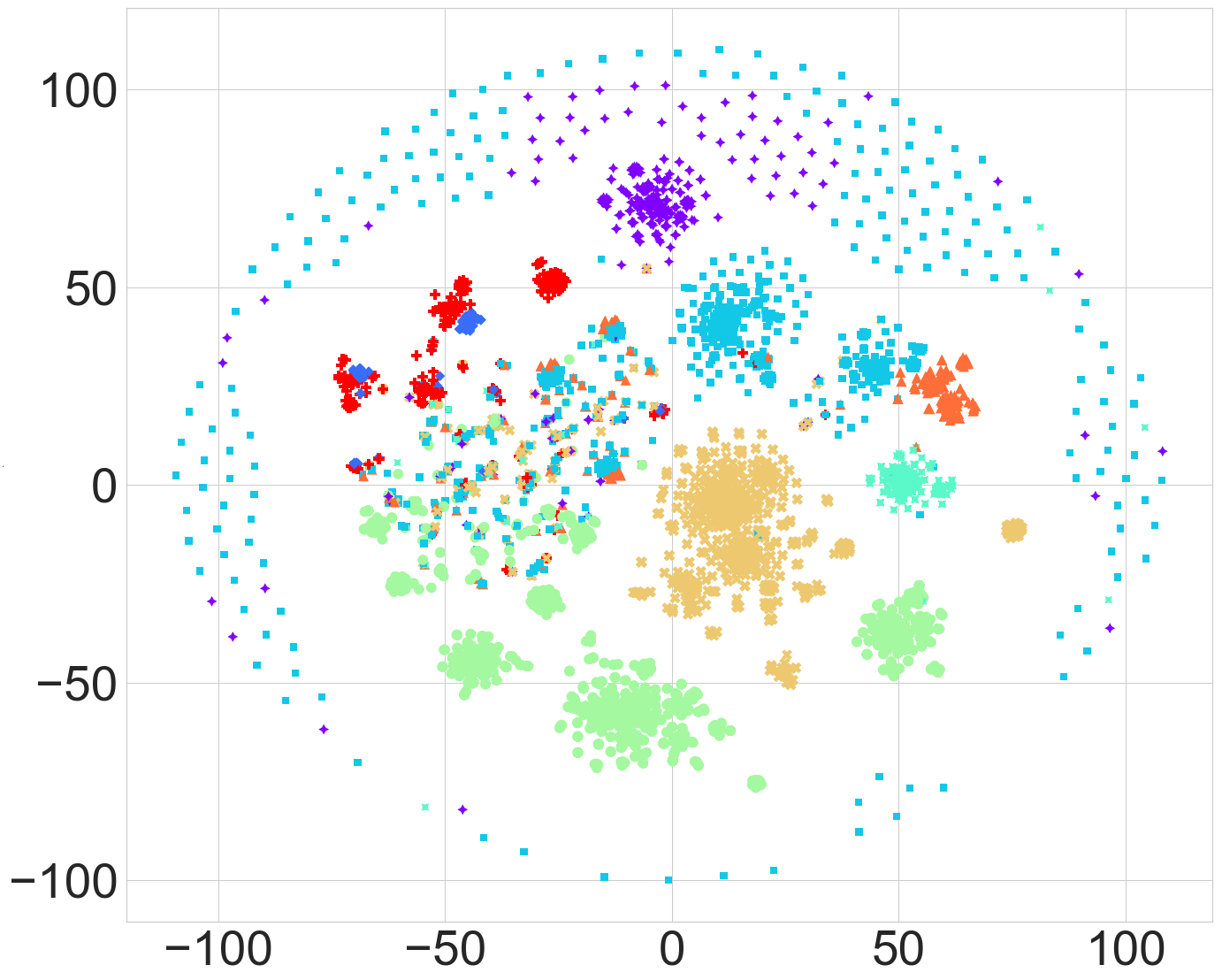
(a) OHE

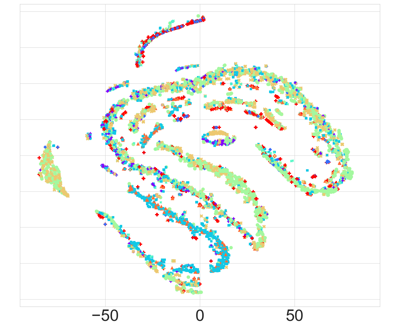
(b) $k$-mers

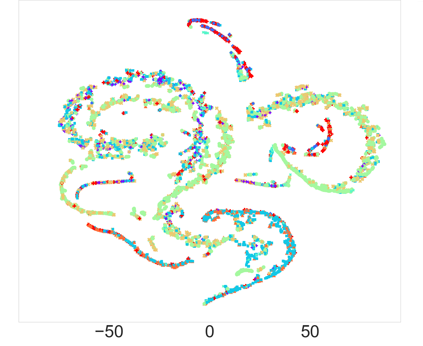
(c) minimizers

Figure 10: t-SNE plots for different embedding methods on real data containing 6812 Sequences (labels by Pangolin). This figure is best seen in color.

5 Results and Discussions

In this section, we first provide all of the results for the experiments on the simulated data following which we report results for the experiments on the real data.

We start with the classification results on the simulated data for the three alignment-free embedding methods mentioned in Section 3.1. Afterward, we present the result after applying SMOTE, explained in Section 3.2, to tackle the class imbalance problem. We then report the clustering results on simulated data for the algorithms listed in Section 3.3, and perform model evaluation using the internal clustering metrics mentioned in Section 3.4 and the cluster comparison metrics of Section 3.5. We show the results and evaluation of clustering for different possible combinations for simulated data. Finally, we perform a statistical analysis using Pearson and Spearman correlation to evaluate the compactness of each feature embedding on the simulated data.

On real data, where there is no ground truth labeling, we perform clustering on such data, evaluating it using the internal clustering metrics mentioned in Section 3.4 and cluster comparison metrics of Section 3.5. We then show, through information gain (IG), that the spike region of the SARS-CoV-2 genome heavily informs the clustering, which is consistent with current biological knowledge its viral structure. Finally, we perform feature importance through Pearson and Spearman correlation to evaluate the compactness of each feature embedding on the real data.

5.1 Results on Simulated Data

This section provides the results of the classification and clustering experiments performed on simulated data.

5.1.1 Classification Results

The classification results for different embedding methods (without SMOTE) are reported in Table 3. We can observe that the proposed Reads2Vec embedding method outperforms all other methods in terms of all evaluation metrics except the training runtime. The average accuracy achieved by Reads2Vec is up to 99.8% and better than the among baseline embeddings where we achieved 98.9% with Spike2Vec.

Table 4 reports the classification with SMOTE for several embedding techniques. We can see that, with the exception of training runtime, the suggested Reads2Vec embedding technique outperforms all other methods in terms of evaluation metrics. However, the average accuracy of Reads2Vec is up marginally because of the smaller room for improvement, but still, we can say that Reads2Vec gives the best results compared with other embeddings.

Method	ML Algo.	Acc.	Prec.	Recall	F1 (Weig.)	F1 (Macro)	ROC AUC	Train Time (Sec.)
Spike2Vec	SVM	0.984 $\pm$ 0.002	0.984 $\pm$ 0.002	0.984 $\pm$ 0.002	0.983 $\pm$ 0.002	0.872 $\pm$ 0.030	0.924 $\pm$ 0.017	0.356 $\pm$ 0.026
	NB	0.102 $\pm$ 0.094	0.662 $\pm$ 0.077	0.102 $\pm$ 0.094	0.146 $\pm$ 0.106	0.066 $\pm$ 0.048	0.535 $\pm$ 0.027	0.038 $\pm$ 0.004
	MLP	0.968 $\pm$ 0.004	0.969 $\pm$ 0.004	0.968 $\pm$ 0.004	0.968 $\pm$ 0.004	0.705 $\pm$ 0.046	0.846 $\pm$ 0.023	2.575 $\pm$ 0.407
	KNN	0.916 $\pm$ 0.006	0.919 $\pm$ 0.005	0.916 $\pm$ 0.006	0.911 $\pm$ 0.006	0.666 $\pm$ 0.034	0.784 $\pm$ 0.022	0.317 $\pm$ 0.047
	RF	0.954 $\pm$ 0.005	0.953 $\pm$ 0.006	0.954 $\pm$ 0.005	0.947 $\pm$ 0.007	0.605 $\pm$ 0.080	0.759 $\pm$ 0.038	2.931 $\pm$ 0.284
	LR	0.989 $\pm$ 0.002	0.988 $\pm$ 0.002	0.989 $\pm$ 0.002	0.988 $\pm$ 0.003	0.851 $\pm$ 0.042	0.915 $\pm$ 0.011	1.572 $\pm$ 0.139
	DT	0.922 $\pm$ 0.004	0.922 $\pm$ 0.005	0.922 $\pm$ 0.004	0.922 $\pm$ 0.004	0.530 $\pm$ 0.037	0.758 $\pm$ 0.018	0.681 $\pm$ 0.063
Minimizers2Vec	SVM	0.981 $\pm$ 0.002	0.981 $\pm$ 0.001	0.981 $\pm$ 0.002	0.981 $\pm$ 0.001	0.862 $\pm$ 0.045	0.935 $\pm$ 0.025	0.28 $\pm$ 0.015
	NB	0.339 $\pm$ 0.086	0.85 $\pm$ 0.036	0.339 $\pm$ 0.086	0.404 $\pm$ 0.093	0.189 $\pm$ 0.048	0.639 $\pm$ 0.033	0.041 $\pm$ 0.003
	MLP	0.973 $\pm$ 0.002	0.972 $\pm$ 0.001	0.973 $\pm$ 0.002	0.972 $\pm$ 0.002	0.741 $\pm$ 0.045	0.865 $\pm$ 0.019	3.231 $\pm$ 0.422
	KNN	0.939 $\pm$ 0.005	0.936 $\pm$ 0.005	0.939 $\pm$ 0.005	0.934 $\pm$ 0.006	0.666 $\pm$ 0.029	0.785 $\pm$ 0.013	0.316 $\pm$ 0.024
	RF	0.97 $\pm$ 0.003	0.968 $\pm$ 0.003	0.97 $\pm$ 0.003	0.966 $\pm$ 0.004	0.675 $\pm$ 0.038	0.801 $\pm$ 0.017	1.279 $\pm$ 0.056
	LR	0.98 $\pm$ 0.001	0.979 $\pm$ 0.002	0.98 $\pm$ 0.001	0.979 $\pm$ 0.001	0.836 $\pm$ 0.045	0.903 $\pm$ 0.028	1.006 $\pm$ 0.072
	DT	0.95 $\pm$ 0.002	0.949 $\pm$ 0.002	0.95 $\pm$ 0.002	0.949 $\pm$ 0.002	0.661 $\pm$ 0.036	0.822 $\pm$ 0.033	0.315 $\pm$ 0.068
Reads2Vec	SVM	0.998 $\pm$ 0.002	0.998 $\pm$ 0.002	0.998 $\pm$ 0.002	0.998 $\pm$ 0.002	0.988 $\pm$ 0.030	0.994 $\pm$ 0.017	1.097 $\pm$ 0.026
	NB	0.125 $\pm$ 0.094	0.727 $\pm$ 0.077	0.125 $\pm$ 0.094	0.195 $\pm$ 0.106	0.089 $\pm$ 0.048	0.553 $\pm$ 0.027	0.184 $\pm$ 0.004
	MLP	0.987 $\pm$ 0.004	0.988 $\pm$ 0.004	0.987 $\pm$ 0.004	0.987 $\pm$ 0.004	0.813 $\pm$ 0.046	0.913 $\pm$ 0.023	2.921 $\pm$ 0.407
	KNN	0.944 $\pm$ 0.006	0.946 $\pm$ 0.005	0.944 $\pm$ 0.006	0.941 $\pm$ 0.006	0.777 $\pm$ 0.034	0.835 $\pm$ 0.022	0.384 $\pm$ 0.047
	RF	0.987 $\pm$ 0.005	0.987 $\pm$ 0.006	0.987 $\pm$ 0.005	0.986 $\pm$ 0.007	0.85 $\pm$ 0.080	0.89 $\pm$ 0.038	4.157 $\pm$ 0.284
	LR	0.998 $\pm$ 0.002	0.998 $\pm$ 0.002	0.998 $\pm$ 0.002	0.998 $\pm$ 0.003	0.973 $\pm$ 0.042	0.98 $\pm$ 0.011	3.761 $\pm$ 0.139
	DT	0.973 $\pm$ 0.004	0.973 $\pm$ 0.005	0.973 $\pm$ 0.004	0.973 $\pm$ 0.004	0.734 $\pm$ 0.037	0.869 $\pm$ 0.018	2.021 $\pm$ 0.063

Table 3: Average $\pm$ standard deviation classification results without SMOTE for real dataset. Best average values are shown in bold.

Method	ML Algo.	Acc.	Prec.	Recall	F1 (Weig.)	F1 (Macro)	ROC AUC	Train Time (Sec.)
Spike2Vec	SVM	0.999 $\pm$ 0	0.999 $\pm$ 0	0.999 $\pm$ 0	0.999 $\pm$ 0	0.999 $\pm$ 0	0.999 $\pm$ 0	3.888 $\pm$ 0.11
	NB	0.301 $\pm$ 0.005	0.388 $\pm$ 0.011	0.301 $\pm$ 0.005	0.229 $\pm$ 0.004	0.229 $\pm$ 0.004	0.607 $\pm$ 0.003	0.194 $\pm$ 0.005
	MLP	0.997 $\pm$ 0	0.997 $\pm$ 0	0.997 $\pm$ 0	0.997 $\pm$ 0	0.997 $\pm$ 0	0.998 $\pm$ 0	5.232 $\pm$ 1.039
	KNN	0.972 $\pm$ 0.001	0.972 $\pm$ 0.001	0.972 $\pm$ 0.001	0.971 $\pm$ 0.001	0.971 $\pm$ 0.001	0.984 $\pm$ 0.001	6.851 $\pm$ 0.274
	RF	0.998 $\pm$ 0.001	0.998 $\pm$ 0.001	0.998 $\pm$ 0.001	0.998 $\pm$ 0.001	0.998 $\pm$ 0.001	0.999 $\pm$ 0	16.187 $\pm$ 0.335
	LR	0.997 $\pm$ 0	0.997 $\pm$ 0	0.997 $\pm$ 0	0.996 $\pm$ 0	0.996 $\pm$ 0	0.998 $\pm$ 0	9.999 $\pm$ 0.38
	DT	0.977 $\pm$ 0.001	0.977 $\pm$ 0.001	0.977 $\pm$ 0.001	0.977 $\pm$ 0.002	0.976 $\pm$ 0.002	0.987 $\pm$ 0.001	2.833 $\pm$ 0.062
Minimizers2Vec	SVM	0.999 $\pm$ 0	0.999 $\pm$ 0	0.999 $\pm$ 0	0.999 $\pm$ 0	0.999 $\pm$ 0	0.999 $\pm$ 0	3.845 $\pm$ 0.445
	NB	0.457 $\pm$ 0.01	0.545 $\pm$ 0.016	0.457 $\pm$ 0.01	0.401 $\pm$ 0.01	0.402 $\pm$ 0.009	0.695 $\pm$ 0.005	0.206 $\pm$ 0.017
	MLP	0.997 $\pm$ 0.001	0.997 $\pm$ 0.001	0.997 $\pm$ 0.001	0.997 $\pm$ 0.001	0.997 $\pm$ 0.001	0.998 $\pm$ 0.001	6.270 $\pm$ 0.877
	KNN	0.980 $\pm$ 0.001	0.980 $\pm$ 0.001	0.980 $\pm$ 0.001	0.980 $\pm$ 0.001	0.980 $\pm$ 0.001	0.989 $\pm$ 0	7.188 $\pm$ 0.483
	RF	0.999 $\pm$ 0	0.999 $\pm$ 0	0.999 $\pm$ 0	0.999 $\pm$ 0	0.999 $\pm$ 0	0.999 $\pm$ 0	8.407 $\pm$ 0.429
	LR	0.991 $\pm$ 0	0.991 $\pm$ 0	0.991 $\pm$ 0	0.991 $\pm$ 0	0.991 $\pm$ 0	0.995 $\pm$ 0	8.817 $\pm$ 0.514
	DT	0.985 $\pm$ 0.002	0.985 $\pm$ 0.002	0.985 $\pm$ 0.002	0.985 $\pm$ 0.002	0.985 $\pm$ 0.002	0.991 $\pm$ 0.001	1.620 $\pm$ 0.228
Reads2Vec	SVM	1 $\pm$ 0	1 $\pm$ 0	1 $\pm$ 0	1 $\pm$ 0	1 $\pm$ 0	1 $\pm$ 0	10.539 $\pm$ 0.314
	NB	0.503 $\pm$ 0.004	0.618 $\pm$ 0.006	0.503 $\pm$ 0.004	0.46 $\pm$ 0.003	0.459 $\pm$ 0.002	0.72 $\pm$ 0.002	1.006 $\pm$ 0.007
	MLP	0.999 $\pm$ 0	0.999 $\pm$ 0	0.999 $\pm$ 0	0.999 $\pm$ 0	0.999 $\pm$ 0	1 $\pm$ 0	3.971 $\pm$ 0.484
	KNN	0.985 $\pm$ 0.001	0.985 $\pm$ 0.001	0.985 $\pm$ 0.001	0.985 $\pm$ 0.001	0.985 $\pm$ 0.001	0.991 $\pm$ 0	8.539 $\pm$ 0.195
	RF	1 $\pm$ 0	1 $\pm$ 0	1 $\pm$ 0	1 $\pm$ 0	1 $\pm$ 0	1 $\pm$ 0	25.257 $\pm$ 0.109
	LR	1 $\pm$ 0	1 $\pm$ 0	1 $\pm$ 0	1 $\pm$ 0	1 $\pm$ 0	1 $\pm$ 0	20.27 $\pm$ 0.438
	DT	0.995 $\pm$ 0.001	0.995 $\pm$ 0.001	0.995 $\pm$ 0.001	0.995 $\pm$ 0.001	0.995 $\pm$ 0.001	0.997 $\pm$ 0	8.411 $\pm$ 0.35

Table 4: Average $\pm$ standard deviation classification results with SMOTE for the real dataset. Best average values are shown in bold (considering 6 decimal places).

5.1.2 Clustering Results

To perform clustering, we use two settings. In the first setting, we select the value for $k$, i.e., the number of clusters, using the elbow method. In the second setting, we select the value for $k$ equal to the total number of unique class labels given by the “ground truth” clustering corresponding to the labels assigned by the Pangolin tool.

Elbow Method Based Results.

The elbow method used to select the optimal number of clusters is given in Figure 11 for all embedding methods. The selected value of $k$ using the elbow method is 5, 5, and 4 for Spike2Vec, Minimizers2Vec, and Reads2Vec, respectively.

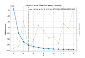
(a) Spike2Vec

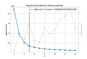
(b) Minimizers2Vec

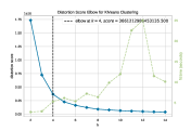
(c) Reads2Vec

Figure 11: Elbow method to determine the number of clusters in the simulated dataset. The selected value of $k$ is 5, 5, and 4 for Spike2Vec, Minimizers2Vec, and Reads2Vec, respectively. This figure is best seen in color.

The clustering results for $k$ selected using elbow method are shown in Table 5. We can observe that in this experimental setting, the Spike2Vec embedding method outperforms the other two methods for all but one evaluation metric. For the Davies-Bouldin Score, the proposed Reads2Vec performs the best. In all cases, the $k$-means algorithm performs better than the $k$-modes clustering algorithm.

		Evaluation Metrics
Algorithm	Embedding	Silhouette Coefficient	Calinski-Harabasz Score	Davies-Bouldin Score	Clustering Runtime (in sec.)
$k$-means	Spike2Vec	0.780	61422.728	0.472	2.980435
	Minimizers2Vec	0.730	48513.248	0.526	4.705328
	Reads2Vec	0.774	48644.237	0.452	12.59896
$k$-mode	Spike2Vec	-0.468	20.500	7.430	82.898802
	Minimizers2Vec	0.345	24.311	24.927	29.893825
	Reads2Vec	0.425	912.212	29.601	542.186639

Table 5: Internal clustering quality metrics on the simulated data for $k$-means and $k$-modes using Spike2Vec ($k=5$), Minimizers2Vec ($k=5$), and Reads2Vec ($k=4$) embeddings. Best values are shown in bold.

The comparison of embeddings with each other using the $k$-means clustering method are shown in Figure 12 using different metrics including ARI, FMI, CD, and VM. We can observe that overall Spike2Vec and Minimizers2Vec are most similar to each other for all comparison metrics. Moreover, Reads2Vec is more similar to Spike2Vec than Minimizers2Vec.

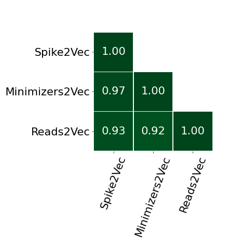
(a) ARI

(b) FMI

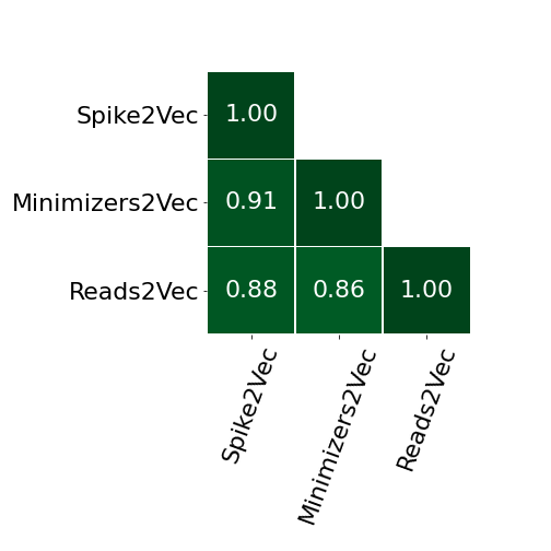
(c) CS

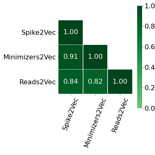
(d) VM

Figure 12: Comparison of $k$-means clustering approaches and embedding methods on the simulated data using standard clustering comparison metrics for $k$ clusters ($k$ selected using elbow method).

Ground Truth Clustering Based Results.

The clustering results for $k$ selected based on the number of clusters in the labeling produced by the Pangolin tool are shown in Table 6. We can observe that in this experimental setting, the Spike2Vec embedding method outperforms the other two methods in all evaluation metrics. In all cases, the $k$-means clustering algorithm performs better than the $k$-modes clustering algorithm.

		Evaluation Metrics
Algorithm	Embedding	Silhouette Coefficient	Calinski-Harabasz Score	Davies-Bouldin Score	Clustering Runtime (in sec.)
ground	OHE	0.315	463.886	1.576	$\approx 18$ hours
$k$-means	Spike2Vec	0.744	92556.901	0.532	4.326378
	Minimizers2Vec	0.635	48097.935	0.724	5.693730
	Reads2Vec	0.736	91182.722	0.535	6.255037
$k$-mode	Spike2Vec	-0.405	17.027	44.572	175.485736
	Minimizers2Vec	0.304	17.693	20.084	49.965804
	Reads2Vec	0.354	512.340	134.516	1447.708700

Table 6: Internal clustering quality metrics on the simulated data for $k$-means and $k$-modes using Spike2Vec, Minimizers2Vec, and Reads2Vec embeddings (in call cases, $k=9$, the number of clusters in the labeling by the Pango tool).

The comparison of different embedding methods with $k=9$ is shown in Figure 13. Here, we also show the “ground truth embedding”, which is the one-hot encoding representation of the sequences. We can observe that Spike2Vec and Reads2Vec are most similar to each other in this case while Minimizers2Vec is also closely related to both Spike2Vec and Reads2Vec. However, the ground truth embedding appears to be very different from the other embedding methods.

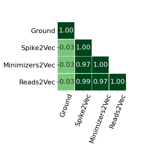
(a) ARI

(b) FMI

(c) CS

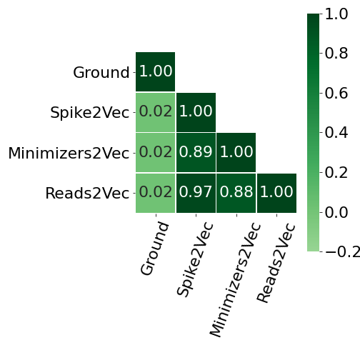
(d) VM

Figure 13: Comparison of $k$means clustering approaches and embedding methods on the simulated dataset using standard clustering comparison metrics for $k=9$ clusters.

5.1.3 Feature Importance

The correlation of features with the class labels using Pearson and Spearman correlation are shown in Figure 14 for the simulated data. In case of Spearman correlation, we can observe that Reads2Vec contains higher correlation with the class labels (lineages) compared to the other embedding methods. However, for Pearson correlation, Spike2Vec contains higher correlation of features with the class labels.

(a) Spearman

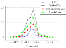
(b) Pearson

Figure 14: Fraction of features in the simulated data correlated with the labeling in the case of Pearson and Spearman.

5.2 Results on Real Data

This section provides the results of the clustering methods using different embedding methods and evaluation metrics performed on real data.

5.2.1 Clustering Evaluation

Table 7 shows the results for different clustering algorithms and their comparison with various embeddings on three internal clustering evaluation metrics. Since Pangolin [Pan] takes sequences as input rather than numerical feature vectors, we cluster the sequences using the Pangolin tool and then we evaluate the quality of the clustering labels using the different numerical embeddings of these sequences. The performance of OHE with the Pangolin labels is better than to the performance of $k$-mers or minimizers with Pangolin labels overall, probably because OHE is a straightforward numerical representation of a sequence (possibly similar to the ML representation that Pangolin uses internally). Moreover, we can observe that the $k$-mers based feature embedding performs better with $k$-means clustering in all but one evaluation metric. An important observation here is that the clustering from $k$-means shows better performance as compared to the Pangolin tool overall. This indicates that the Pangolin tool may not be the best option in this raw high-throughput sequencing reads setting. We observe that the $k$-modes clustering algorithm performs poorly in most cases for clustering and runtime.

		Evaluation Metrics
Algorithm	Embedding	Silhouette Coefficient	Calinski-Harabasz Score	Davies-Bouldin Score	Clustering Runtime
Pangolin	OHE	0.029	818.673	8.471
	$k$-mers	-0.214	78.098	7.864	$\approx 14$ hours
	minimizers	-0.233	144.200	6.063
$k$-means	OHE	0.623	3278.376	1.502	648.5 Sec.
	$k$-mers	0.775	21071.221	0.406	19.2 Sec.
	minimizers	0.858	17909.284	0.421	31.3 Sec.
$k$-modes	OHE	0.613	2053.754	2.056	$\approx 7$ days
	$k$-mers	-0.027	9.801	89.789	$\approx 4$ hours
	minimizers	-0.398	1196.777	3.545	$\approx 1$ hour

Table 7: Internal clustering quality metrics for Pangolin, $k$-means and $k$-modes on OHE, $k$-mers and minimizers embeddings on the real data. Best values are shown in bold.

5.2.2 Comparing Different Clusterings

We compare the different clustering algorithms on different embeddings using the adjusted Rand index (ARI), Fowlkes-Mallows index (FMI), V-measure (VM) and completeness score (CS). The heat map in Figure 15 shows that some embeddings are more similar to others. We observe that the $k$-mers + $k$-means combination is very similar to the minimizers + $k$-means combination in terms of ARI, FMI, VM and CS. This shows that the clusterings from the combinations of clustering method and embedding are not much different from each other.

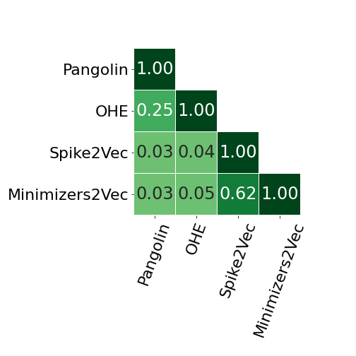
(a) ARI

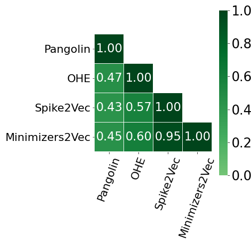
(b) FMI

(c) CS

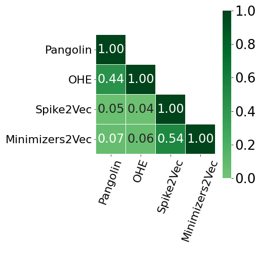
(d) VM

Figure 15: Comparison of different embedding methods on the real data for $k$-means clustering using standard clustering comparison metrics.

5.2.3 Information Gain

The combination of clustering method and embedding which performed the best overall, in terms of internal clustering quality, was $k$-mers + $k$-means (see Table 7). To verify if such a clustering makes sense from a biological standpoint, thereby independently validating such a clustering from an orthogonal viewpoint, we also computed the importance of each genomic position in the sequence to the labeling (the clustering) obtained by $k$-mers + $k$-means. For this purpose, we computed the Information Gain (IG) of this labeling in terms of genomic position, defined as:

$$IG(\mbox{class},\mbox{position})=H(\mbox{class})-H(\mbox{class}~{}|~{}\mbox{position})$$ (1)

where

$$H(\mbox{class})=\sum_{e\in\mbox{class}}-p_{e}\log p_{e}$$ (2)

is the entropy of a class in terms of the proportion of each unique label $e$ of this class. Figure 16 shows the IG values for different genomic positions corresponding to the class labels. We can see that many positions have higher IG values, which means that they play an important role in predicting the labels.

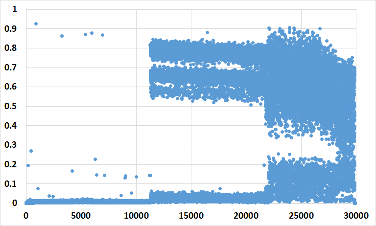
Figure 16: Information gain values for different genomic positions. The x-axis shows the position and the y-axis shows the information gain value.

This IG scatter plot partitions the SARS-CoV-2 genome into three distinct regions, with very low IG (0–11Kbp), with either very high or very low IG (11Kbp–22Kbp), and with a wide range of IG (22Kbp–30Kbp). What is interesting is that the structural proteins S, E, M and N [WPT⁺20] fall in the $21$Kbp–$25$Kbp range, overlapping, for the most part, this third region with the wide range of IG. This is consistent with the observation that mutations of the SARS-CoV-2 genome (which define many of the different variants) appear disproportionately in the structural proteins region, particularly the spike (S) region [XWYZ20].

5.2.4 Statistical Analysis

Since the information gain is in terms of positions of the genomic sequence, it does not provide information on how important the features of each embedding are (since feature vectors are in the Euclidean space). For this purpose, we use Spearman and Pearson correlation to evaluate the (negative and positive) importance of features in the different embeddings. Since we note from the previous Section 5.2.2 that the combination of $k$-mers + $k$-means is quite similar to minimizers + $k$-means, we performed such an analysis on the consensus (agreement of both clusterings) labels from both clusterings. A total of 5738 labels and the corresponding feature embedding were analyzed.

Spearman Correlation.

We use Spearman correlation [MS04] to evaluate the contribution of different attributes of feature embeddings. The Spearman Correlation is computed using the following expression:

$$\rho=1-\frac{6\sum d_{i}^{2}}{n(n^{2}-1)}~{},$$ (3)

where $\rho$ is the Spearman’s rank correlation coefficient, $d_{i}$ is the difference between the two ranks of each observation, and $n$ is the total number of observations.

The number of features having negative and positive Spearman correlation for the different ranges for different embedding methods are shown in Figure 17 (a) for negative and the positive correlation range. In terms of negative correlation, we can observe that there is only a small fraction of features in the case of OHE. At the same time, other embeddings do not have any features which are negatively correlated to the consensus labeling. In the case of positive correlation, we can observe that the $k$-mers based embedding has more features with high correlation values than the other embeddings. This indicates that the feature embedding from $k$-mers is more compact than OHE and the minimizers based feature embedding approach.

Pearson Correlation.

We also use Pearson correlation [BCHC09] to evaluate the compactness of different feature embeddings. The Pearson correlations are shown in Figure 17 (b) for the negative and the positive correlation range. In the case of negative correlation, we can observe that OHE has more features corresponding to the consensus labeling, with a higher Pearson correlation. However, in the case of positive correlation, the $k$-mers based feature vector seems to be more compact than OHE and minimizers based feature embedding.

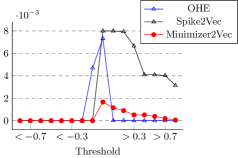
(a) Spearman

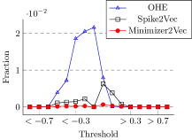
(b) Pearson

Figure 17: Fraction of features correlated with the labeling on the real data in the case of Spearman and Pearson. This figure is best seen in color.

6 Conclusion

In this paper, we propose an efficient alignment-free feature vector embedding approach, Reads2Vec, for the setting of raw high-throughput reads data. Such embedding is used as input to different supervised (i.e., classification) and unsupervised (i.e., clustering) methods for different machine learning-based tasks. We perform experiments on both real-world and simulated short read data related to the coronavirus, SARS-CoV-2. We show that Reads2Vec outperforms other alignment-free baselines in terms of predictive performance on the classification task. Using different clustering evaluation metrics, we indicate that alignment-free embeddings are more suited to this raw sequencing reads setting than the widely accepted Pangolin tool. Finally, in computing the information gain (IG), we show that most of the genomic positions having high IG corresponding to the labeling (from the clustering) are concentrated in the spike region of the SARS-CoV-2 genome, which is consistent with current biological knowledge this virus.

In the future, we would explore the scalability of such approaches by using more data. Another direction of future work is to explore how sensitive the predictions of the Pangolin tool, or OHE are to the genome assembly. Finally, we would like to explore the usage of such embedding in conjunction with alignment-free variant calling, which could possibly eliminate even more dependencies on the genome assembly step.

Author Contribution Statement

SC, MP: Conceptualization. SA: Methodology. PC, SA, MP: Software. PC, SA: Validation. PC, SA: Formal Analysis. All: Investigation. All: Resources. MP: Data Curation. All: Writing - Original Draft. All: Writing - Review & Editing. PC, SA: Visualization. GDV, MP: Supervision. GDV, MP: Administration. SA, GDV, MP: Funding Acquisition.

Conflict of Interest

The authors declare no conflict of interest.

Funding Statement

Research supported by an MBD Fellowship for SA, and a Georgia State University Computer Science start-up grant for MP. This project has received funding from the European Union’s Horizon 2020 Research and Innovation Staff Exchange programme under the Marie Skłodowska-Curie grant agreement No. 872539.

References

- [AAF+20] Sarwan Ali, Maria Khalid Alvi, Safi Faizullah, Muhammad Asad Khan, Abdullah Alshanqiti, and Imdadullah Khan. Detecting ddos attack on sdn due to vulnerabilities in openflow. In International Conference on Advances in the Emerging Computing Technologies (AECT), pages 1–6, 2020.
- [AAK+21] Sarwan Ali, Tamkanat E Ali, Muhammad Asad Khan, Imdadullah Khan, and Murray Patterson. Effective and scalable clustering of sars-cov-2 sequences. In International Conference on Big Data Research (ICBDR), pages 42–49, 2021.
- [AAT+20] Muhammad Ahmad, Sarwan Ali, Juvaria Tariq, Imdadullah Khan, Mudassir Shabbir, and Arif Zaman. Combinatorial trace method for network immunization. Information Sciences, 519:215–228, 2020.
- [ABC+22] Sarwan Ali, Babatunde Bello, Prakash Chourasia, Ria Thazhe Punathil, Yijing Zhou, and Murray Patterson. PWM2Vec: An efficient embedding approach for viral host specification from coronavirus spike sequences. Biology, 11(3):418, 2022.
- [AMAK19] Sarwan Ali, Haris Mansoor, Naveed Arshad, and Imdadullah Khan. Short term load forecasting using smart meter data. In Proceedings of the Tenth ACM International Conference on Future Energy Systems, pages 419–421, 2019.
- [AMK+19] Sarwan Ali, Haris Mansoor, Imdadullah Khan, Naveed Arshad, Muhammad Asad Khan, and Safiullah Faizullah. Short-term load forecasting using ami data. arXiv preprint arXiv:1912.12479, 2019.
- [AP21] Sarwan Ali and Murray Patterson. Spike2vec: An efficient and scalable embedding approach for covid-19 spike sequences. In IEEE International Conference on Big Data (Big Data), pages 1533–1540, 2021.
- [ASK+21] Sarwan Ali, Muhammad Haroon Shakeel, Imdadullah Khan, Safiullah Faizullah, and Muhammad Asad Khan. Predicting attributes of nodes using network structure. ACM Transactions on Intelligent Systems and Technology (TIST), 12(2):1–23, 2021.
- [ASK+22] Sarwan Ali, Bikram Sahoo, Muhammad Asad Khan, Alexander Zelikovsky, Imdad Ullah Khan, and Murray Patterson. Efficient approximate kernel based spike sequence classification. IEEE/ACM Transactions on Computational Biology and Bioinformatics, 2022.
- [ASU+21] Sarwan Ali, Bikram Sahoo, Naimat Ullah, Alexander Zelikovskiy, Murray Patterson, and Imdadullah Khan. A k-mer based approach for sars-cov-2 variant identification. In International Symposium on Bioinformatics Research and Applications, pages 153–164, 2021.
- [AZP22] Sarwan Ali, Yijing Zhou, and Murray Patterson. Efficient analysis of covid-19 clinical data using machine learning models. Medical & Biological Engr. & Computing, pages 1–16, 2022.
- [BCHC09] Jacob Benesty, Jingdong Chen, Yiteng Huang, and Israel Cohen. Pearson correlation coefficient. In Noise reduction in speech processing, pages 1–4. 2009.
- [Bla86] B. Blaisdell. A measure of the similarity of sets of sequences not requiring sequence alignment. Proceedings of the National Academy of Sciences, 83:5155–5159, 1986.
- [BSK15] Karel Břinda, Maciej Sykulski, and Gregory Kucherov. Spaced seeds improve -mer-based metagenomic classification. Bioinformatics, 31:3584–3592, 2015.
- [CBHK02] Nitesh V Chawla, Kevin W Bowyer, Lawrence O Hall, and W Philip Kegelmeyer. Smote: synthetic minority over-sampling technique. Journal of artificial intelligence research, 16:321–357, 2002.
- [CH74] Tadeusz Calinski and Jerzy Harabasz. A dendrite method for cluster analysis. Communications in Statistics-theory and Methods, 3(1):1–27, 1974.
- [DB79] David Davies and Donald Bouldin. A cluster separation measure. IEEE transactions on pattern analysis and machine intelligence, (2):224–227, 1979.
- [DBL+] Petr Danecek, James Bonfield, Jennifer Liddle, John Marshall, et al. Twelve years of SAMtools and BCFtools. GigaScience, 10(2).
- [DPMZ+21] Louis Du Plessis, John McCrone, Alexander Zarebski, et al. Establishment and lineage dynamics of the sars-cov-2 epidemic in the uk. Science, 371(6530):708–712, 2021.
- [FM83] Edward B Fowlkes and Colin L Mallows. A method for comparing two hierarchical clusterings. Journal of the American statistical association, 78(383):553–569, 1983.
- [GHE18] Hayer J Gourlé H, Karlsson-Lindsjö O and Bongcam-Rudloff E. Simulating Illumina data with InSilicoSeq. Bioinformatics, 2018.
- [GIS22] GISAID Website. https://www.gisaid.org/, 2022.
- [GPC16] Samuele Girotto, Cinzia Pizzi, and Matteo Comin. Metaprob: accurate metagenomic reads binning based on probabilistic sequence signatures. Bioinformatics, 32(17):i567–i575, 2016.
- [GWEJ07] Tanya Golubchik, Michael Wise, Simon Easteal, and Lars Jermiin. Mind the gaps: Evidence of bias in estimates of multiple sequence alignments. Molecular Biology and Evolution, 24(11):2433–2442, 2007.
- [HA85] Lawrence Hubert and Phipps Arabie. Comparing partitions. Journal of classification, 2(1):193–218, 1985.
- [HMB+18] James Hadfield, Colin Megill, Sidney M Bell, et al. Nextstrain: real-time tracking of pathogen evolution. Bioinformatics, 34(23):4121–4123, 2018.
- [Hua98] Zhexue Huang. Extensions to the k-means algorithm for clustering large data sets with categorical values. Data mining and knowledge discovery, 2(3):283–304, 1998.
- [K+20] K. Kuzmin et al. Machine learning methods accurately predict host specificity of coronaviruses based on spike sequences alone. Biochemical and Biophysical Research Communications, 533(3):553–558, 2020.
- [KD15] Jolanta Kawulok and Sebastian Deorowicz. Cometa: classification of metagenomes using k-mers. PloS one, 10(4):e0121453, 2015.
- [Li13] Heng Li. Aligning sequence reads, clone sequences and assembly contigs with BWA-MEM. arXiv preprint arXiv:1303.3997, 2013.
- [LJL+20] XW Liang, AP Jiang, T Li, YY Xue, and GT Wang. Lr-smote—an improved unbalanced data set oversampling based on k-means and svm. Knowledge-Based Systems, 196:105845, 2020.
- [Llo82] Stuart Lloyd. Least squares quantization in pcm. IEEE transactions on information theory, 28(2):129–137, 1982.
- [M+21] Felix Mölder et al. Sustainable data analysis with snakemake. F1000Research, 10, 2021.
- [MES16] Alejandro Moreo, Andrea Esuli, and Fabrizio Sebastiani. Distributional random oversampling for imbalanced text classification. In Proceedings of the 39th International ACM SIGIR conference on Research and Development in Information Retrieval, pages 805–808, 2016.
- [MMK+21] Andrew Melnyk, Fatemeh Mohebbi, Sergey Knyazev, Bikram Sahoo, Roya Hosseini, Pavel Skums, Alex Zelikovsky, and Murray Patterson. From alpha to zeta: Identifying variants and subtypes of sars-cov-2 via clustering. Journal of Comp Biology, 28(11):1113–1129, 2021.
- [MS04] Leann Myers and Maria Sirois. Spearman correlation coefficients, differences between. Encyclopedia of statistical sciences, 12, 2004.
- [MS+20] Bui Quang Minh, Heiko A Schmidt, et al. Iq-tree 2: new models and efficient methods for phylogenetic inference in the genomic era. Molecular biology and evolution, 37(5):1530–1534, 2020.
- [OSU+21] Aine O’Toole, Emily Scher, Anthony Underwood, et al. Assignment of epidemiological lineages in an emerging pandemic using the pangolin tool. Virus Evolution, 7(2):veab064, 2021.
- [P+11] F. Pedregosa et al. Scikit-learn: Machine learning in Python. Journal of Machine Learning Research, 12:2825–2830, 2011.
- [Pan] Pangolin Website. Phylogenetic Assignment of Named Global Outbreak Lineages (Pangolin). https://cov-lineages.org/resources/pangolin.html. [Online; accessed 4-Jan-2022].
- [QPTZ20] M. Queyrel, E. Prifti, A. Templier, and J. Zucker. Towards end-to-end disease prediction from raw metagenomic data. bioRxiv, 2020.
- [Rep] Staff Reporter. CDC commits $90m to create public health pathogen genomics research centers. Genomeweb. [Online; accessed 29-September-2022].
- [RH07] A. Rosenberg and J. Hirschberg. V-measure: A conditional entropy-based external cluster evaluation measure. In the Joint Conf. Empirical Methods NLP Computational Natural Language Learning (EMNLP-CoNLL), pages 410–420, 2007.
- [RHH+04] Michael Roberts, Wayne Hayes, Brian Hunt, Stephen Mount, and James Yorke. Reducing storage req for biological sequence comparison. Bioinformatics, 20(18):3363–3369, 2004.
- [RHO+20] Andrew Rambaut, Edward Holmes, A. O’Toole, et al. A dynamic nomenclature proposal for SARS-CoV-2 lineages to assist genomic epi. Nature Microbiology, 5(11):1403–1407, 2020.
- [Rou87] Peter Rousseeuw. Silhouettes: a graphical aid to interpretation and validation of cluster analysis. Journal of computational and applied mathematics, 20:53–65, 1987.
- [S+15] Zachary Stephens et al. Big data: astronomical or genomical? PLoS biology, 13(7):e1002195, 2015.
- [SAIR11] Ville Satopaa, Jeannie Albrecht, David Irwin, and Barath Raghavan. Finding a” kneedle” in a haystack: Detecting knee points in system behavior. In International conference on distributed computing systems workshops, pages 166–171, 2011.
- [SMG+11] A. Sboner, X. Mu, D. Greenbaum, R. Auerbach, and M. Gerstein. The real cost of sequencing: higher than you think! Genome Biology, 12(8):125, 2011.
- [SRAPK18] Stephen Solis-Reyes, Mariano Avino, Art Poon, and Lila Kari. An open-source k-mer based machine learning tool for fast and accurate subtyping of hiv-1 genomes. PloS one, 13(11):e0206409, 2018.
- [SS+17] Ritambhara Singh, Arshdeep Sekhon, et al. Gakco: a fast gapped k-mer string kernel using counting. In Joint ECML and Knowledge Discovery in Databases, pages 356–373, 2017.
- [TAP21] Zahra Tayebi, Sarwan Ali, and Murray Patterson. Robust representation and efficient feature sel allows for effective clustering of sars-cov-2 variants. Algorithms, 14(12):348, 2021.
- [UAK+20] Asad Ullah, Sarwan Ali, Imdadullah Khan, Muhammad Asad Khan, and Safiullah Faizullah. Effect of analysis window and feature selection on classification of hand movements using emg signal. In Proceedings of SAI Intelligent Systems Conference, pages 400–415. Springer, 2020.
- [VdMH08] Laurens Van der Maaten and Geoffrey Hinton. Visualizing data using t-sne. Journal of machine learning research, 9(11), 2008.
- [WPT+20] Alexandra C Walls, Young-Jun Park, M Alejandra Tortorici, Abigail Wall, Andrew T McGuire, and David Veesler. Structure, function, and antigenicity of the sars-cov-2 spike glycoprotein. Cell, 181(2):281–292, 2020.
- [WS14] Derrick E Wood and Steven L Salzberg. Kraken: ultrafast metagenomic sequence classification using exact alignments. Genome biology, 15(3):1–12, 2014.
- [XWYZ20] Wenxin Xu, Mingjie Wang, Demin Yu, and Xinxin Zhang. Variations in sars-cov-2 spike protein cell epitopes and glycosylation profiles during global transmission course of covid-19. Frontiers in Immunology, 11, 2020.
- [YKZZ17] Xuebing Yang, Qiuming Kuang, Wensheng Zhang, and Guoping Zhang. Amdo: An over-sampling technique for multi-class imbalanced problems. IEEE Transactions on Knowledge and Data Engineering, 30(9):1672–1685, 2017.