Few-Shot Inductive Learning on Temporal Knowledge Graphs using Concept-Aware Information

Abstract

Knowledge graph completion (KGC) aims to predict the missing links among knowledge graph (KG) entities. Though various methods have been developed for KGC, most of them can only deal with the KG entities seen in the training set and cannot perform well in predicting links concerning novel entities in the test set. Similar problem exists in temporal knowledge graphs (TKGs), and no previous temporal knowledge graph completion (TKGC) method is developed for modeling newly-emerged entities. Compared to KGs, TKGs require temporal reasoning techniques for modeling, which naturally increases the difficulty in dealing with novel, yet unseen entities. In this work, we focus on the inductive learning of unseen entities’ representations on TKGs. We propose a few-shot out-of-graph (OOG) link prediction task for TKGs, where we predict the missing entities from the links concerning unseen entities by employing a meta-learning framework and utilizing the meta-information provided by only few edges associated with each unseen entity. We construct three new datasets for TKG few-shot OOG link prediction, and we propose a model that mines the concept-aware information among entities. Experimental results show that our model achieves superior performance on all three datasets and our concept-aware modeling component demonstrates a strong effect.

1 Introduction

Knowledge graphs (KGs) store factual information in the form of triples, i.e., $(s,r,o)$, where $s$, $o$, $r$ denote the subject entity, the object entity, and the relation between them, respectively. KGs have already been widely used in a series of downstream tasks, e.g., question answering Saxena et al. (2020); Ding et al. (2022b) and recommender systems Wang et al. (2019c, a). While KG triples are capable of representing facts, they cannot express their time validity. World knowledge is ever-changing, which means many facts have their own time validity, e.g., the fact (Angela Merkel, is chancellor of, Germany) is valid only before (Olaf Scholz, is chancellor of, Germany). To this end, temporal knowledge graphs (TKGs) are introduced to consider the time validity of facts by representing every fact with a quadruple, i.e., $(s,r,o,t)$, where $t$ denotes the time when the fact is valid.

KGs and TKGs are known to suffer from incompleteness Min et al. (2013); Leblay and Chekol (2018). Therefore, various methods have been developed for automatically completing KGs Nickel et al. (2011); Bordes et al. (2013); Trouillon et al. (2016); Sun et al. (2019); Guo and Kok (2021) and TKGs Tresp et al. (2015); Leblay and Chekol (2018); Ma et al. (2019); Jung et al. (2021); Ding et al. (2021). Though these methods achieve superior performance on knowledge graph completion (KGC) and temporal knowledge graph completion (TKGC), they have their limitations. In real-world scenarios, KGs and TKGs evolve over time, indicating that new (unseen) entities may emerge constantly Shi and Weninger (2018). Besides, real-world KGs exhibit long-tail distributions, where a large portion of entities only have few edges Baek et al. (2020). This also applies to TKGs, e.g., the entity frequency distribution of ICEWS datasets (Appendix A). Traditional KGC and TKGC methods learn the representations of the observed (seen) entities, and perform link prediction over a fixed set of entities. To learn the optimal representations of the observed entities, these methods require a large number of training examples associated with each of them. Baek et al. (2020) shows that traditional KGC methods show poor performance when they are used to predict the links concerning newly-emerged, yet unseen entities. In our work, we also observe that traditional TKGC methods share the same problem (Section 5.3).

To tackle the limitations of traditional TKGC methods, we propose the TKG few-shot out-of-graph (OOG) link prediction task and a TKG reasoning model for better learning the inductive representations of newly-emerged entities in TKGs. Inspired by recent work that mines shared concepts of stocks for improving stock prediction Li et al. (2020); Xu et al. (2021b), we devise a module, taking advantage of the entity concepts provided by the temporal knowledge bases. The contribution of our work is three-folded:

• We propose the TKG few-shot out-of-graph (OOG) link prediction task. To better learn the inductive representations of unseen entities and predict their links, we propose a meta-learning-based model. To the best of our knowledge, this is the first work aiming to improve the link prediction performance concerning unseen entities in TKGs.

• We extract the entity concepts from the temporal knowledge bases and take them as additional information to boost our model performance. We design an effective module to learn concept-aware information. The experimental results show that introducing such information helps to learn better representations for unseen entities in the inductive setting.

• We propose three new datasets for TKG few-shot OOG link prediction, i.e., ICEWS14-OOG, ICEWS18-OOG and ICEWS0515-OOG. We compare our model with several baseline methods. Experimental results show that our model outperforms all the baselines on all three datasets.

2 Related Work

Knowledge graph embedding methods.

Knowledge graph embedding (KGE) methods can be split into two categories. Some methods design scoring functions to compute the plausibility scores of KG facts Bordes et al. (2013); Trouillon et al. (2016); Sun et al. (2019); Guo and Kok (2021), while other KGE methods employ neural-based structures, e.g., graph neural networks (GNNs), to better capture the structural dependencies of KGs Schlichtkrull et al. (2018); Vashishth et al. (2020); Yu et al. (2021). By combining neural-based graph encoders with KG scoring functions, these methods achieve superior performance in KG reasoning tasks.

Temporal knowledge graph embedding methods.

To deal with the temporal constraints in TKG facts, two lines of temporal knowledge graph embedding (TKGE) methods have been developed. The first line of methods designs novel time-aware scoring functions for characterizing extra time information Leblay and Chekol (2018); Ma et al. (2019); Lacroix et al. (2020); Sadeghian et al. (2021); Han et al. (2020a, 2021c). The second line of methods models temporal information by employing neural structures, e.g., GNNs and recurrent models. Han et al. (2021a); Jung et al. (2021); Ding et al. (2021); Han et al. (2020b); Sun et al. (2021) sample every entity’s temporal neighbors and use GNNs to learn time-aware representations of them. Wu et al. (2020) and Han et al. (2021b) model structural information with GNNs, and they achieve temporal reasoning by utilizing a gated recurrent unit Cho et al. (2014) and a neural ordinary differential equation Chen et al. (2018), respectively.

Inductive learning on knowledge graphs.

Traditional KGE and TKGE methods require a large number of training examples to learn entity representations. However, in real-world scenarios, KGs and TKGs are ever-evolving, and they exhibit long-tail distributions. New entities and relations emerge and a huge portion of them only have very few associated facts, thus causing traditional methods unable to learn optimal representations. To alleviate this problem, a line of work Xiong et al. (2018); Chen et al. (2019); Sheng et al. (2020); Mirtaheri et al. (2021); Ding et al. (2022a) tries to employ meta-learning to learn inductive representations of unseen KG (or TKG) relations. Nevertheless, they are unable to deal with novel entities. Several methods try to deal with unseen (out-of-graph) entities in an inductive setting Hamaguchi et al. (2017); Wang et al. (2019b); He et al. (2020). They first learn representations of seen entities, and then use an auxiliary set to transfer knowledge from seen to unseen entities during inference. Baek et al. (2020) proposes a more realistic task: few-shot out-of-graph (OOG) link prediction, where the links among unseen entities are also considered during evaluation and the representation of every unseen entity can only be derived from very few (number of shot size) edges. Baek et al. simulate the unseen entities in the training phase and introduce meta-learning for learning unseen entities’ representations. Based on it, Zhang et al. (2021) proposes a model using hyper-relation features to improve performance on few-shot OOG link prediction. Another series of work tries to include external information of entities, e.g., textual descriptions, to solve this problem Xie et al. (2016); Wang et al. (2019d) and it turns out to be effective in modeling unseen entities. Though there exist various methods dealing with OOG unseen entities in KGs, there is still no method specifically designed to embed unseen entities inductively for TKGs.

3 Preliminaries and Task Formulation

Entity concepts in temporal knowledge graphs.

Entity concepts describe the characteristics of KG entities. They are manually defined by humans and assigned to every KG entity. In the ICEWS database Boschee et al. (2015), entities belong to several sectors, e.g., Government, Executive Office. Each entity’s sectors are specified in the ICEWS weekly event data. We treat the sectors of an entity as its concepts and learn concept representations as additional information. We observe that some region entities in the ICEWS database, e.g., South Korea and North America, have no specified sectors. We manually assign a new sector Region to them. We ensure that every entity has its own sectors. More details about concept extraction is presented in Appendix F.

Task formulation.

We first give the definition of a temporal knowledge graph, then we formulate the TKG few-shot out-of-graph link prediction task.

Definition 1 (Temporal Knowledge Graph (TKG)). Let $\mathcal{E}$, $\mathcal{R}$ and $\mathcal{T}$ denote a finite set of entities, relations and timestamps, respectively. A temporal knowledge graph (TKG) $\mathcal{G}$ can be taken as a finite set of TKG facts represented by their associated quadruples, i.e., $\mathcal{G}=\{(s,r,o,t)|s,o\in\mathcal{E},r\in\mathcal{R},t\in\mathcal{T}\}\subseteq\mathcal{E}\times\mathcal{R}\times\mathcal{E}\times\mathcal{T}$.

Definition 2 (Temporal Knowledge Graph Few-Shot Out-of-Graph Link Prediction). Given an observed background TKG $\mathcal{G}_{\text{back}}\subseteq\mathcal{E}_{\text{back}}\times\mathcal{R}\times\mathcal{E}_{\text{back}}\times\mathcal{T}$, an unseen entity $e^{\prime}$ is an entity $e^{\prime}\in\mathcal{E}^{\prime}$, where $\mathcal{E}^{\prime}\cap\mathcal{E}_{\text{back}}=\emptyset$. Assume we further observe $K$ associated quadruples for each unseen entity $e^{\prime}$ in the form of $(e^{\prime},r,\tilde{e},t)$ (or $(\tilde{e},r,e^{\prime},t)$), where $\tilde{e}\in(\mathcal{E}_{\text{back}}\cup\mathcal{E}^{\prime})$, $r\in\mathcal{R}$, $t\in\mathcal{T}$, and $K$ is a small number denoting the shot size, e.g., 1 or 3. TKG few-shot out-of-graph link prediction aims to predict the missing entities from the link prediction queries $(e^{\prime},r_{q},?,t_{q})$ (or $(?,r_{q},e^{\prime},t_{q})$) derived from unobserved quadruples containing unseen entities, where $r_{q}\in\mathcal{R}$, $t_{q}\in\mathcal{T}$.

We further formulate the TKG few-shot OOG link prediction task into a meta-learning problem. For a TKG $\mathcal{G}\subseteq\mathcal{E}\times\mathcal{R}\times\mathcal{E}\times\mathcal{T}$, we first select a group of entities $\mathcal{E}^{\prime}$, where each entity’s number of associated quadruples is between a lower and a higher threshold. We aim to pick out the entities that are not frequently mentioned in TKG facts since newly-emerged entities normally are coupled with only several edges. We randomly split these entities into three groups $\mathcal{E}^{\prime}_{\text{meta-train}}$, $\mathcal{E}^{\prime}_{\text{meta-valid}}$ and $\mathcal{E}^{\prime}_{\text{meta-test}}$. For each group, we treat the union of all the quadruples associated to this group’s entities as the corresponding meta-learning set, e.g., the meta-training set $\mathbb{T}_{\text{meta-train}}$ is formulated as $\{(e^{\prime},r,\tilde{e},t)|\tilde{e}\in\mathcal{E},r\in\mathcal{R},e^{\prime}\in\mathcal{E}^{\prime}_{\text{meta-train}},t\in\mathcal{T}\}\cup\{(\tilde{e},r,e^{\prime},t)|\tilde{e}\in\mathcal{E},r\in\mathcal{R},e^{\prime}\in\mathcal{E}^{\prime}_{\text{meta-train}},t\in\mathcal{T}\}$. We ensure that there exists no link between every two of the meta-learning sets. The associated quadruples of the rest entities form a background graph $\mathcal{G}_{\text{back}}\subseteq\mathcal{E}_{\text{back}}\times\mathcal{R}\times\mathcal{E}_{\text{back}}\times\mathcal{T}$, where $\mathcal{E}^{\prime}\cap\mathcal{E}_{\text{back}}=\emptyset$ and $\mathcal{E}=(\mathcal{E}_{\text{back}}\cup\mathcal{E}^{\prime})$. We take the meta-training entities $\mathcal{E}^{\prime}_{\text{meta-train}}$ as simulated unseen entities and try to learn how to transfer knowledge from seen entities $\mathcal{E}_{\text{back}}$ to them during meta-training. The entities in $\mathcal{E}^{\prime}_{\text{meta-valid}}$ and $\mathcal{E}^{\prime}_{\text{meta-test}}$ are real unseen entities that are used to evaluate the model performance.

Based on Baek et al. (2020), we define a meta-training task $T$ as follows. In each task $T$, we first randomly sample $N$ simulated unseen entities $\mathcal{E}_{T}$ from $\mathcal{E}^{\prime}_{\text{meta-train}}$. Then we randomly select $K$ associated quadruples for each $e^{\prime}\in\mathcal{E}_{T}$ as its support quadruples $\mathcal{S}_{e^{\prime}}=\{(e^{\prime},r_{i},\tilde{e}_{i},t_{i})\ \text{or}\ (\tilde{e}_{i},r_{i},e^{\prime},t_{i})\}^{K}_{i=1}$, where $K$ is the shot size and $\tilde{e}_{i}\in(\mathcal{E}_{\text{back}}\cup\mathcal{E}^{\prime})$. The rest of $e^{\prime}$’s quadruples are taken as its query quadruples $\mathcal{Q}_{e^{\prime}}=\{(e^{\prime},r_{i},\tilde{e}_{i},t_{i})\ \text{or}\ (\tilde{e}_{i},r_{i},e^{\prime},t_{i})\}^{M_{e^{\prime}}}_{i=K+1}$, where $M_{e^{\prime}}$ denotes the number of $e^{\prime}$’s associated quadruples in $\mathbb{T}_{\text{meta-train}}$ and $\tilde{e}_{i}\in(\mathcal{E}_{\text{back}}\cup\mathcal{E}^{\prime})$. For every meta-training task $T$, the aim of TKG few-shot OOG link prediction is to simultaneously predict the missing entities from the link prediction queries derived from the query quadruples associated to all the entities from $\mathcal{E}_{T}$, e.g., $(e^{\prime},r_{i},?,t_{i})$ or $(?,r_{i},e^{\prime},t_{i})$. In this way, we simulate the situation that we simultaneously observe a bunch of unseen entities and each of them has only few edges, which is similar to how emerging entities appear in temporal knowledge bases. After meta-training, we validate our model on a meta-validation set $\mathbb{T}_{\text{meta-valid}}$ and test our model on a meta-test set $\mathbb{T}_{\text{meta-test}}$, where they contain all the quadruples associated to the entities in $\mathcal{E}^{\prime}_{\text{meta-valid}}$ and $\mathcal{E}^{\prime}_{\text{meta-test}}$, respectively. We do not sample $N$ entities during meta-validation and meta-test. Instead, we treat all the entities in $\mathcal{E}^{\prime}_{\text{meta-valid}}$ (or $\mathcal{E}^{\prime}_{\text{meta-test}}$) as appearing at the same time. For a better understanding, we present Figure 5 to illustrate how we formulate the TKG few-shot OOG link prediction task into a meta-learning problem. We also discuss the difference between our proposed task and traditional TKGC in Appendix D.

We summarize the challenge of TKG few-shot OOG link prediction as follows: (1) TKG reasoning models are asked to predict the links concerning the newly-emerged entities that are completely unseen during the training process; (2) Only a small number ($K$) of edges associated with each newly-emerged entity are observable to support predicting the unobserved links concerning this entity.

4 Our Method

Figure 1: Model structure of FILT. Assume we have an unseen entity $e^{\prime}$, and we want to predict a link corresponding to $(e^{\prime},r_{i},\tilde{e}_{i},t_{i})\in\mathcal{Q}_{e^{\prime}}$. We derive the concept representations in the concept modeling component and use a time difference-based graph encoder for learning $e^{\prime}$’s time-aware representation. We take the representations of $r_{i}$ and $\tilde{e}_{i}$ to compute the plausibility score of the link.

We propose a model dealing with few-shot inductive learning on TKGs (FILT). Figure 1 shows the model structure of FILT. It consists of three components: (1) Concept modeling component that represents entity concepts based on seen entities’ representations; (2) Time difference-based graph encoder that learns the contextualized representations of unseen entities; (3) KG scoring function that computes the plausibility scores of the TKG quadruples concerning unseen entities.

4.1 Concept Modeling Component

When a new entity emerges in a TKG, though there might be only few observed associated edges, some of its concepts, e.g., which sectors it belongs to, are already known. Since every entity concept is shared across all the entities in this TKG, we can learn concept information from seen entities and transfer it to newly-emerged entities.

Inspired by Xu et al. (2021b) that mines concept-aware information for stock prediction, we develop a concept modeling component to learn TKG entity concepts as follows. First, we pre-train our background graph with ComplEx Trouillon et al. (2016). Note that only seen entities $\mathcal{E}_{\text{back}}$ are involved in the pre-training process. Assume we have a set of entity concepts $\mathcal{C}$, then we initialize the representation of every entity concept $c\in\mathcal{C}$ with its associated entities by averaging these entities’ representations:

$$\mathbf{h}_{c}=\frac{1}{|\mathcal{N}_{c}|}\sum_{e\in\mathcal{N}_{c}}\mathbf{h}_{e},$$ (1)

where $\mathbf{h}_{c}$ and $\mathbf{h}_{e}$ denote the representations of the concept $c$ and the entity $e$, respectively. $\mathcal{N}_{c}$ denotes the neighborhood of the entity concept $c$. For example, if two TKG entities Angela Merkel and Xi Jinping both belong to the concept Elite, they will be included into Elite’s neighborhood. Since we want to distinguish the contributions of different entities to an entity concept, we then correct the concept representations as follows:

$$\mathbf{h}_{c}=\sum_{e_{i}\in\mathcal{N}_{c}}\alpha_{c}^{e_{i}}\mathbf{h}_{e_{i}},\quad\alpha_{c}^{e_{i}}=\frac{\exp(\mathbf{h}^{\top}_{e_{i}}\mathbf{h}_{c})}{\sum_{e_{j}\in\mathcal{N}_{c}}\exp(\mathbf{h}^{\top}_{e_{j}}\mathbf{h}_{c})}.$$ (2)

After we correct the concept representations, we compute an entity’s concept-aware information by aggregating the representations of its associated concepts:

$$\mathbf{h}_{e}^{\mathcal{C}_{e}}=\sum_{c_{i}\in\mathcal{C}_{e}}\beta_{e}^{c_{i}}\mathbf{h}_{c_{i}},\quad\beta_{e}^{c_{i}}=\frac{\exp(\mathbf{h}^{\top}_{c_{i}}\mathbf{h}_{e})}{\sum_{c_{j}\in\mathcal{C}_{e}}\exp(\mathbf{h}^{\top}_{c_{j}}\mathbf{h}_{e})}.$$ (3)

$\mathcal{C}_{e}\subseteq\mathcal{C}$ denotes the set of all concepts associated to $e$. As shown in Figure 1, we inject the concept-aware information into two branches. We use two separate layers of feed forward neural network and project the concept-aware information onto two branches. The upper branch adds the concept information to the entity representations $\mathbf{h}_{e}:=\mathbf{h}_{e}+\delta_{1}\sigma(\mathbf{W}_{c}^{1}\mathbf{h}_{e}^{\mathcal{C}_{e}})$ and take them as the input of our graph encoder. The lower branch processes the concept information $\delta_{2}\sigma(\mathbf{W}_{c}^{2}\mathbf{h}_{e}^{\mathcal{C}_{e}})$ and adds it to the entity representations after the graph aggregation step. $\delta_{1}$ and $\delta_{2}$ are two trainable weights deciding how much concept-aware information should be injected. $\mathbf{W}_{c}^{1}$ and $\mathbf{W}_{c}^{2}$ are two weight matrices and $\sigma$ is an activation function. By employing the double branch structure, we not only include the concept information into the graph encoder, but also directly infuse it into the final entity representations for link prediction.

4.2 Time Difference-Based Graph Encoder

Figure 2: The structure of the time difference-based graph encoder. Assume we have an unseen entity Chongwadai, and we have a link prediction query (Chongwadai, Engage in negotiation, $?$, 2014-07-24), given three support quadruples, i.e., (North Korea, Make an appeal or request, Chongwadai, 2014-09-22), (Chongwadai, Make statement, Grand National Party, 2014-06-05), and (Chongwadai, Make statement, Barak Obama, 2014-04-04). We use our graph encoder to compute the time-aware contextualized representation of Chongwadai at 2014-07-24. For each temporal neighbor from a support quadruple, we compute its importance according to the time difference between 2014-07-24 and the timestamp of its corresponding support quadruple. We denote the temporal neighbors with colored circles. The color darkness of the circles implies the importance of the temporal neighbors during aggregation in Equation 4. The darker circle a temporal neighbor is represented with, the more important it is, i.e., $\gamma_{q}^{2}>\gamma_{q}^{1}>\gamma_{q}^{3}$.

To compute the contextualized representations of the unseen entities, we employ a time difference-based graph encoder. For each unseen entity $e^{\prime}$, assume we have a link prediction query $(e^{\prime},r_{q},?,t_{q})$ derived from a query quadruple $(e^{\prime},r_{q},\tilde{e}_{q},t_{q})\in\mathcal{Q}_{e^{\prime}}$. We first find its temporal neighbors from its support quadruples $\mathcal{S}_{e^{\prime}}=\{(e^{\prime},r_{i},\tilde{e}_{i},t_{i})\ \text{or}\ (\tilde{e}_{i},r_{i},e^{\prime},t_{i})\}^{K}_{i=1}$, and then compute $e^{\prime}$’s time-aware representation at $t_{q}$ through aggregation:

$$\mathbf{h}_{(e^{\prime},t_{q})}=\sum_{(\tilde{e}_{i},r_{i},t_{i})\in\mathcal{N}_{e^{\prime}}}\gamma_{q}^{i}\mathbf{W_{g}}(\mathbf{h}_{\tilde{e}_{i}}\|\mathbf{h}_{r_{i}}),\quad\gamma_{q}^{i}=\frac{\exp(1/{|t_{q}-t_{i}|})}{\sum_{(\tilde{e}_{j},r_{j},t_{j})\in\mathcal{N}_{e^{\prime}}}\exp(1/|t_{q}-t_{j}|)}.$$ (4)

$\mathbf{W}_{g}$ denotes the weight matrix in our graph encoder. $\mathcal{N}_{e^{\prime}}$ denotes the observed neighborhood of $e^{\prime}$ and $|\mathcal{N}_{e^{\prime}}|=K$. $\gamma_{q}^{i}$ is the importance of the $i$th temporal neighbor $\tilde{e}_{i}$ based on the time difference between $t_{q}$ and $t_{i}$. The smaller the time difference is, the more important a temporal neighbor is during aggregation. The motivation of our time difference-based graph encoder is that we assume the temporal neighbors that are temporally closer to the query timestamp $t_{q}$ tend to contribute more to predicting the links at $t_{q}$. Since we take the temporal neighbors of an entity from its incoming edges, we transform every support quadruple whose form is $(e^{\prime},r_{i},\tilde{e}_{i},t_{i})$ to $(\tilde{e}_{i},r^{-1}_{i},e^{\prime},t_{i})$, where $r^{-1}_{i}$ corresponds to the inverse relation of $r_{i}$. We manage to incorporate every support quadruple into the aggregation process with this quadruple transformation. Note that if $t_{q}-t_{i}=0$, the denominator of the exponential term will be $0$. Thus, we use a constant $\lambda$ to assign a value to $\exp(1/{|t_{q}-t_{i}|})$ if $t_{q}$ equals $t_{i}$, and $\lambda$ serves as a hyperparameter that can be tuned. Figure 2 illustrates the structure of our graph encoder with an example. After aggregation, we further infuse the concept-aware information from the lower branch into the output of our graph encoder: $\mathbf{h}_{(e^{\prime},t_{q})}:=\mathbf{h}_{(e^{\prime},t_{q})}+\delta_{2}\sigma(\mathbf{W}_{c}^{2}\mathbf{h}_{e^{\prime}}^{\mathcal{C}_{e^{\prime}}})$. We show in Section 5.4 that our simple-structured graph encoder can beat more complicated structures in the TKG OOG link prediction task.

4.3 Parameter Learning

For each meta-training task $T$, we have $N$ simulated unseen entities $\mathcal{E}_{T}$. We use the hinge loss for learning model parameters:

$$\mathcal{L}=\sum_{e^{\prime}\in\mathcal{E}_{T}}\sum_{q^{+}\in\mathcal{Q}_{e^{\prime}}}\sum_{q^{-}\in\mathcal{Q}^{-}_{e^{\prime}}}\text{max}\{\theta-score(q^{+})+score(q^{-}),0\}.$$ (5)

$\theta>0$ is the margin. $q^{+}$ denotes a query quadruple from $e^{\prime}$’s query set. $q^{-}$ is generated by negative sampling Bordes et al. (2013). For every $q^{+}=(e^{\prime},r_{q},\tilde{e}_{q},t_{q})$ (or $q^{+}=(\tilde{e}_{q},r_{q},e^{\prime},t_{q})$), we corrupt $\tilde{e}_{q}$ with another entity $e^{-}\in\{\mathcal{E}^{\prime},\mathcal{E}_{\text{back}}\}$. We map our learned representations to the complex space and use ComplEx Trouillon et al. (2016) as our scoring function, i.e., $score=\text{Re}<\mathbf{h}_{s},\mathbf{h}_{r},\bar{\mathbf{h}}_{o}>$, where $\mathbf{h}_{s}$, $\mathbf{h}_{o}$ denote the representations of the subject entity and the object entity, respectively. $\mathbf{h}_{r}$ denotes the relation representation. Re means taking the real part, and $\bar{\mathbf{h}}_{o}$ means taking the conjugate of the vector $\mathbf{h}_{o}$.

5 Experiments

We compare FILT with several baselines on TKG few-shot OOG link prediction. To prove the effectiveness of the model components, we conduct several ablation studies. We also do further analysis to show the robustness of our method. Besides, we visualize the learned concept representations and show that our concept modeling component helps to capture the semantics of entity concepts.

5.1 Datasets

We propose three TKG few-shot OOG link prediction datasets, i.e., ICEWS14-OOG, ICEWS18-OOG, and ICEWS0515-OOG. We first take three subsets, i.e., ICEWS14, ICEWS18, and ICEWS05-15, from the Integrated Crisis Early Warning System (ICEWS) database Boschee et al. (2015), where they contain the timestamped political facts in 2014, in 2018, and from 2005 to 2015, respectively. Following the data construction process of Baek et al. (2020), for each subset, we first randomly sample half of the entities whose number of associated quadruples is between a lower and a higher threshold as unseen entities. Then we split the sampled entities into three groups $\mathcal{E}^{\prime}_{\text{meta-train}}$, $\mathcal{E}^{\prime}_{\text{meta-valid}}$, $\mathcal{E}^{\prime}_{\text{meta-test}}$ ($\mathcal{E}^{\prime}_{\text{meta-train}}\cap\mathcal{E}^{\prime}_{\text{meta-valid}}=\emptyset$, $\mathcal{E}^{\prime}_{\text{meta-train}}\cap\mathcal{E}^{\prime}_{\text{meta-test}}=\emptyset$, $\mathcal{E}^{\prime}_{\text{meta-valid}}\cap\mathcal{E}^{\prime}_{\text{meta-test}}=\emptyset$), where $|\mathcal{E}^{\prime}_{\text{meta-train}}|:|\mathcal{E}^{\prime}_{\text{meta-valid}}|:|\mathcal{E}^{\prime}_{\text{meta-test}}|\approx 8:1:1$. The associated quadruples of all the entities in $\mathcal{E}^{\prime}_{\text{meta-train}}$/$\mathcal{E}^{\prime}_{\text{meta-valid}}$/$\mathcal{E}^{\prime}_{\text{meta-test}}$ form the meta-training/meta-validation/meta-test set. The rest of the quadruples without unseen entities are used for constructing a background graph $\mathcal{G}_{\text{back}}$. The dataset statistics are presented in Table 1. We present the dataset construction process in Appendix H.

Dataset	$|\mathcal{E}|$	$|\mathcal{R}|$	$|\mathcal{T}|$	$|\mathcal{E}^{\prime}_{\text{meta-train}}|$	$|\mathcal{E}^{\prime}_{\text{meta-valid}}|$	$|\mathcal{E}^{\prime}_{\text{meta-test}}|$	$N_{\text{back}}$	$N_{\text{meta-train}}$	$N_{\text{meta-valid}}$	$N_{\text{meta-test}}$
ICEWS14-OOG	7128	230	365	385	48	49	83448	5772	718	705
ICEWS18-OOG	23033	256	304	1268	160	158	444269	19291	2425	2373
ICEWS0515-OOG	10488	251	4017	647	80	82	448695	10115	1217	1228

Table 1: Dataset statistics. $|\mathcal{E}^{\prime}_{\text{meta-train}}|$, $|\mathcal{E}^{\prime}_{\text{meta-valid}}|$, $|\mathcal{E}^{\prime}_{\text{meta-test}}|$ denote the number of unseen entities in the meta-training set, meta-validation set, meta-test set, respectively. $N_{\text{back}}$ denotes the number of quadruples in the background graph $\mathcal{G}_{\text{back}}$. $N_{\text{meta-train}}$, $N_{\text{meta-valid}}$, $N_{\text{meta-test}}$ denote the number of quadruples concerning unseen entities in $\mathbb{T}_{\text{meta-train}}$, $\mathbb{T}_{\text{meta-valid}}$, $\mathbb{T}_{\text{meta-test}}$, respectively.

5.2 Baseline Methods

We take four types of methods as our baselines. First we consider two traditional KGC methods, i.e., ComplEx Trouillon et al. (2016) and BiQUE Guo and Kok (2021). Then we consider several traditional TKGC methods, i.e., TNTComplEx Lacroix et al. (2020), TeLM Xu et al. (2021a), and TeRo Xu et al. (2020a). We combine all the quadruples in the background graph $\mathcal{G}_{\text{back}}$ with the quadruples of the meta-training set to construct a training set for traditional KGC as well as TKGC methods, and let them evaluate on all the query quadruples in the meta-validation/meta-test set. We also include two inductive KGC methods for OOG link prediction that do not employ meta-learning framework, i.e., MEAN Hamaguchi et al. (2017), LAN Wang et al. (2019b). To achieve fair comparison, we only allow them to utilize support quadruples during inference, rather than an auxiliary set containing a large number of quadruples for each unseen entity $e^{\prime}\in\{\mathcal{E}^{\prime}_{\text{meta-valid}},\mathcal{E}^{\prime}_{\text{meta-test}}\}$. Apart from the first three types of methods, we further consider a meta-learning-based method GEN Baek et al. (2020) which deals with few-shot OOG link prediction on static KGs. For the baseline methods designed for static KGs, we provide them with all the quadruples in our datasets and neglect time constraints, i.e., neglecting $t$ in $(s,r,o,t)$. We ensure that all the methods evaluate exactly the same quadruples.

5.3 Experimental Results

We report the TKG 1-shot and 3-shot OOG link prediction results in Table 2. We use mean reciprocal rank (MRR) and Hits@1/3/10 as the evaluation metrics (definition in Appendix B). We follow the filtered setting Bordes et al. (2013) for fairer evaluation. We observe that traditional KGC and TKGC methods show inferior performance in predicting the links concerning unseen entities. This is due to their nature that they have no way to transfer knowledge from seen to unseen entities. Besides, they learn representations of seen entities with a large number of associated training examples, thus causing the learned representations more prone to the data concerning seen entities and failing to embed unseen entities inductively. We also observe that inductive learning methods for static KGs show degenerated performance. MEAN, LAN, heavily rely on the auxiliary set during inference. We constrain their auxiliary set to only include the support quadruples, where only 1 associated quadruple for each unseen entity is included in the 1-shot case (3 associated quadruples in the 3-shot case). Experimental results show that these methods cannot effectively deal with newly-emerged entities that have only few observed edges, which is common in real-world scenarios. GEN employs meta-learning during training, thus having the ability to alleviate the data sparsity problem. However, it has no component to model temporal information, and it also does not incorporate any additional information, e.g., textual information and concept-aware information. To this end, GEN underperforms FILT in both 1-shot and 3-shot cases. Another crucial point worth noting is that the margin between FILT and GEN is much larger in the 3-shot case than in the 1-shot case. We attribute this to our time difference-based graph encoder. Our encoder distinguishes the importance of multiple support quadruples and aggregates the temporal neighbors more effectively.

Datasets	ICEWS14-OOG								ICEWS18-OOG								ICEWS0515-OOG
	MRR		H@1		H@3		H@10		MRR		H@1		H@3		H@10		MRR		H@1		H@3		H@10
Model	1-S	3-S	1-S	3-S	1-S	3-S	1-S	3-S	1-S	3-S	1-S	3-S	1-S	3-S	1-S	3-S	1-S	3-S	1-S	3-S	1-S	3-S	1-S	3-S
ComplEx	.048	.046	.018	.014	.045	.046	.099	.089	.039	.044	.031	.026	.048	.042	.085	.093	.077	.076	.045	.048	.074	.071	.129	.120
BiQUE	.039	.035	.015	.014	.041	.030	.073	.066	.029	.032	.022	.021	.033	.037	.064	.073	.075	.083	.044	.049	.072	.077	.130	.144
TNTComplEx	.043	.044	.015	.016	.033	.042	.102	.096	.046	.048	.023	.026	.043	.044	.087	.082	.034	.037	.014	.012	.031	.036	.060	.071
TeLM	.032	.035	.012	.009	.021	.023	.063	.077	.049	.019	.029	.001	.045	.013	.084	.054	.080	.072	.041	.034	.077	.072	.138	.151
TeRo	.009	.010	.002	.002	.005	.002	.015	.020	.007	.006	.003	.001	.006	.003	.013	.006	.012	.023	.000	.010	.008	.017	.024	.040
MEAN	.035	.144	.013	.054	.032	.145	.082	.339	.016	.101	.003	.014	.012	.114	.043	.283	.019	.148	.003	.039	.017	.175	.052	.384
LAN	.168	.199	.050	.061	.199	.255	.421	.500	.077	.127	.018	.025	.067	.165	.199	.344	.171	.182	.081	.068	.180	.191	.367	.467
GEN	.231	.234	.162	.155	.250	.284	.378	.389	.171	.216	.112	.137	.189	.252	.289	.351	.268	.322	.185	.231	.308	.362	.413	.507
FILT	.278	.321	.208	.240	.305	.357	.410	.475	.191	.266	.129	.187	.209	.298	.316	.417	.273	.370	.201	.299	.303	.391	.405	.516

Table 2: TKG 1-shot and 3-shot OOG link prediction results. Evaluation metrics are filtered MRR and Hits@1/3/10 (H@1/3/10). The best results are marked in bold.

5.4 Ablation Study

To prove the effectiveness of the model components, we conduct several ablation studies on ICEWS14-OOG and ICEWS18-OOG. We devise model variants in the following way. (A) Concept Modeling Variants: In A1 we run our model without the concept modeling component. In A2, we delete the lower branch connecting the concept modeling component with the output of the graph encoder. In A3, we delete the upper branch connecting the concept modeling component with the input of the graph encoder. (B) Graph Encoder Variants: In B1, we neglect the time information and switch our graph encoder to RGCN Schlichtkrull et al. (2018). In B2, we use Time2Vec Kazemi et al. (2019) to model temporal information. In B3, we employ the functional time encoder introduced in Xu et al. (2020b) as our graph encoder. In B4, we derive a time-aware attentional network as our graph encoder: $\mathbf{h}_{(e^{\prime},t_{q})}=\sum_{(\tilde{e}_{i},r_{i},t_{i})\in\mathcal{N}_{e^{\prime}}}\gamma_{q}^{i}\mathbf{W}_{g}(\mathbf{h}_{\tilde{e}_{i}}\|\mathbf{h}_{r_{i}})$, where $\gamma_{q}^{i}=\frac{\exp\left(\sigma\left(([\mathbf{h}_{r_{q}}\|\Phi(t_{q})]\mathbf{W}_{Q})^{\top}([\mathbf{h}_{r_{i}}\|\Phi(t_{i})]\mathbf{W}_{K})\right)\right)}{\sum_{(\tilde{e}_{j},r_{j},t_{j})\in\mathcal{N}_{e^{\prime}}}\exp\left(\sigma\left(([\mathbf{h}_{r_{q}}\|\Phi(t_{q})]\mathbf{W}_{Q})^{\top}([\mathbf{h}_{r_{j}}\|\Phi(t_{j})]\mathbf{W}_{K})\right)\right)}$. $\Phi$ denotes the functional time encoder proposed in Xu et al. (2020b) and $\mathbf{W}_{Q}$, $\mathbf{W}_{K}$ are two weight matrices.

We report the experimental results of the ablation studies in Table 3. From A1 to A3, we show that our concept modeling component helps to improve model performance, and it benefits from its double branch structure. From B1, we find that incorporating temporal information into the graph encoder is important for modeling TKGs. Besides, B2 to B4 show that in TKG few-shot OOG link prediction, it is not necessary to employ a complicated graph encoding structure. A possible reason is that we can only observe $K$ (1 or 3) associated quadruples for every unseen entity, and this forms a tiny neighborhood. Complicated structures, e.g., our time-aware attentional network, are unable to demonstrate their superiority in this case.

Datasets	ICEWS14-OOG						ICEWS18-OOG
	MRR		H@1		H@10		MRR		H@1		H@10
Model	1-S	3-S	1-S	3-S	1-S	3-S	1-S	3-S	1-S	3-S	1-S	3-S
A1	.267	.302	.195	.220	.407	.462	.187	.261	.128	.181	.315	.408
A2	.271	.285	.203	.217	.403	.454	.188	.265	.129	.187	.316	.411
A3	.276	.306	.206	.235	.401	.471	.189	.265	.125	.185	.316	.415
B1	.243	.256	.171	.179	.361	.402	.184	.238	.122	.162	.314	.383
B2	.258	.281	.181	.196	.393	.432	.185	.240	.119	.165	.316	.388
B3	.249	.278	.177	.179	.389	.438	.183	.242	.116	.166	.314	.395
B4	.263	.284	.192	.195	.400	.450	.181	.245	.112	.174	.307	.393
FILT	.278	.321	.208	.240	.410	.475	.191	.266	.129	.187	.316	.417

Table 3: Ablation studies of FILT on ICEWS14-OOG and ICEWS18-OOG. H@1/3/10 denote Hits@1/3/10, respectively. The best results are marked in bold.

5.5 Further Analysis

Cross shot analysis.

We evaluate our trained 3-shot and 1-shot models with varying shots (1,3 or 5-shot) during meta-test. We observe in Table 4 that for both trained models, the performance increases as the test shot size rises. This is due to the effectiveness of our time-aware graph encoder. It distinguishes the importance of different support quadruples and better incorporates graph information as the shot size increases. We also observe that when the test shot size is larger than 3, FILT trained with 3 shots performs better than it trained with 1 shot. This is because during 3-shot meta-training, we simulate that for every unseen entity, 3 support examples are observable, which helps the model to generalize to the cases where their shot sizes are larger than 1 during meta-test. Besides, test with random shots does not greatly affect our model performance, thus showing FILT’s robustness.

Datasets	ICEWS14-OOG						ICEWS18-OOG						ICEWS0515-OOG
	(Train) 1-shot			(Train) 3-shot			(Train) 1-shot			(Train) 3-shot			(Train) 1-shot			(Train) 3-shot
Test Shots	MRR	H@1	H@10	MRR	H@1	H@10	MRR	H@1	H@10	MRR	H@1	H@10	MRR	H@1	H@10	MRR	H@1	H@10
1-shot	.278	.208	.410	.265	.195	.386	.191	.129	.316	.178	.117	.305	.273	.201	.405	.258	.184	.399
3-shot	.293	.212	.452	.321	.240	.475	.232	.158	.381	.266	.187	.417	.331	.254	.482	.370	.299	.516
5-shot	.297	.212	.467	.322	.231	.503	.256	.183	.400	.289	.206	.449	.351	.275	.499	.394	.317	.553
R-shot	.283	.203	.440	.299	.214	.462	.224	.154	.364	.242	.167	.390	.315	.240	.460	.337	.262	.490

Table 4: Cross shot analysis results. R-shot denotes the setting that we randomly sample 1, 3 or 5 support quadruples for every unseen entity during meta-test. H@1/3/10 denote Hits@1/3/10, respectively.

Visualization of concept representations.

We plot the trained concept representations of the 3-shot model on ICEWS18-OOG with t-SNE Van der Maaten and Hinton (2008). The entity concepts in the ICEWS database are hierarchical. For example, under the concept Government, there exist other concepts, e.g., Foreign Ministry. We only create labels for the first hierarchy concepts and assign other concepts belonging to them with the same label. From Figure 3, we can observe that the concepts bearing the same label tend to form a cluster, and the clusters having similar semantic meanings tend to be close to each other, e.g., the clusters of Parties and Government. This demonstrates that our concept modeling component learns the semantics of entity concepts, which helps to improve inductive learning for unseen new entities. We present three case studies in Appendix G.

Figure 3: Visualization of learned concept representations on 3-shot ICEWS18-OOG.

6 Conclusion

We propose a new task: temporal knowledge graph (TKG) few-shot out-of-graph (OOG) link prediction, aiming to introduce the inductive entity representation learning problem into TKGs. We develop a model that focuses on the few-shot inductive learning on TKGs (FILT). Given only few edges associated to each newly-emerged entity, FILT employs a meta-learning framework that enables inductive knowledge transfer from seen entities to new unseen entities. FILT uses a time-aware graph encoder to learn the contextualized representations of unseen entities, which shows stronger performance as the shot size increases. It also utilizes the external entity concept information specified in the temporal knowledge bases. We propose three new datasets for TKG few-shot OOG link prediction and compare FILT with several baselines. Experimental results show that learning concept-aware information improves inductive learning for emerging entities. In the future, we would like to generalize rule-based knowledge graph reasoning methods to the TKG inductive learning scenario. Another direction is to combine future link prediction with our proposed TKG few-shot OOG link prediction task since our task currently does not support link forecasting.

A Long-Tail Distribution of Entities in Temporal Knowledge Bases

Figure A illustrates the entity occurrence of ICEWS14, ICEWS18 and ICEWS05-15 databases. We find that most entities occur for only a few times.

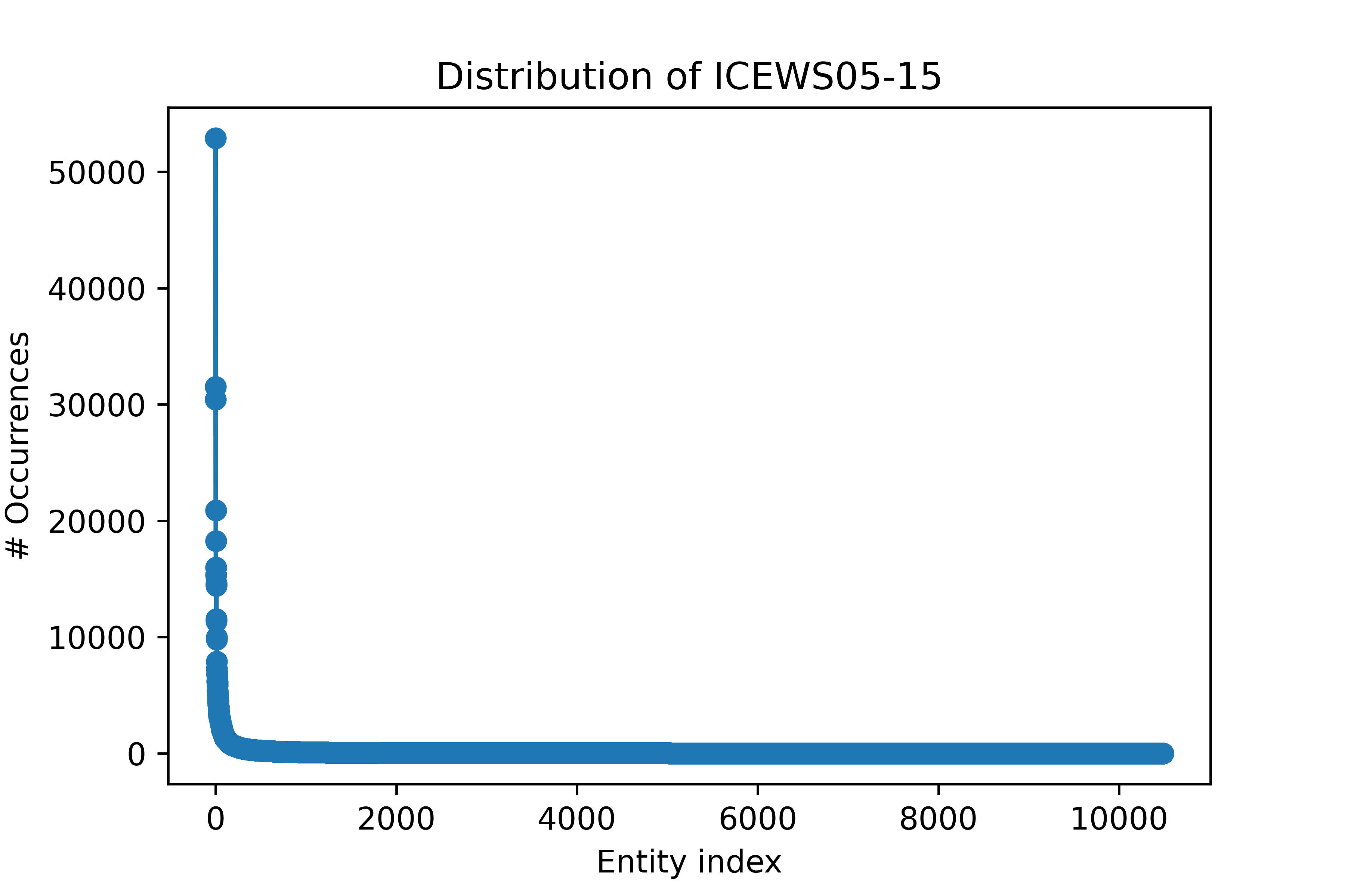
Figure 4: Entity occurrence of ICEWS14, ICEWS18 and ICEWS05-15 databases.

B Evaluation Metrics

We use two evaluation metrics for our experiments, i.e., mean reciprocal rank (MRR) and Hits@1/3/10. For every link prediction query, we compute the rank $\psi$ of the ground truth missing entity. MRR is defined as: $\frac{1}{\sum_{e^{\prime}\in\mathcal{E}^{\prime}_{\text{meta-test}}}|\mathcal{Q}_{e^{\prime}}|}\sum_{e^{\prime}\in\mathcal{E}^{\prime}_{\text{meta-test}}}\sum_{q^{+}\in\mathcal{Q}_{e^{\prime}}}\frac{1}{\psi}$. Hits@1/3/10 denote the proportions of the predicted links where ground truth missing entities are ranked as top 1, top3, top10, respectively.

C Implementation Details

We implement all the experiments with PyTorch Paszke et al. [2019] on a single NVIDIA Tesla T4. We search hyperparameters following Table 6. For each dataset, we do 108 trials to try different hyperparameter settings. We run 15000 batches for each trail and compare their meta-validation results. We choose the setting leading to the best meta-validation result and take it as the best hyperparameter setting. We report the best hyperparameter setting in Table 6. Every result of our model is the average result of five runs. For the models leading to the results reported in Table 2, we provide their meta-validation results in Table 7. We also specify their GPU memory usage (Table 9) and number of parameters (Table 9). For different datasets, we use different numbers of unseen entities $N$ in each meta-training task $T$. We set $N=100$ for ICEWS14-OOG and ICEWS0515-OOG, $N=200$ for ICEWS18-OOG. We sample 32 negative samples for every positive sample.

Hyperparameter	Search Space
Embedding Size	{50, 100, 200}
# Aggregation Step	{1, 2}
Activation Function	{Tanh, ReLU, LeakyReLU}
Dropout	{0.2, 0.3, 0.5}
$\lambda$	{0.2, 0.4}

Table 5: Hyperparameter searching strategy.

Datasets	ICEWS14-OOG	ICEWS18-OOG	ICEWS0515-OOG
Hyperparameter
Embedding Size	100	100	100
# Aggregation Step	1	1	1
Activation Function	LeakyReLU	LeakyReLU	LeakyReLU
Dropout	0.3	0.3	0.3
$\lambda$	0.2	0.4	0.4

Table 6: Best hyperparameter settings.

Datasets	ICEWS14-OOG								ICEWS18-OOG								ICEWS0515-OOG
	MRR		H@1		H@3		H@10		MRR		H@1		H@3		H@10		MRR		H@1		H@3		H@10
Model	1-S	3-S	1-S	3-S	1-S	3-S	1-S	3-S	1-S	3-S	1-S	3-S	1-S	3-S	1-S	3-S	1-S	3-S	1-S	3-S	1-S	3-S	1-S	3-S
FILT	.251	.354	.171	.271	.285	.389	.410	.511	.187	.242	.127	.163	.204	.264	.308	.406	.232	.316	.163	.229	.247	.350	.378	.491

Table 7: TKG 1-shot and 3-shot OOG link prediction results on the meta-validation set. Evaluation metrics are filtered MRR and Hits@1/3/10 (H@1/3/10).

Datasets	ICEWS14-OOG		ICEWS18-OOG		ICEWS0515-OOG
	GPU Memory		GPU Memory		GPU Memory
Model	1-S	3-S	1-S	3-S	1-S	3-S
FILT	1493MB	1466MB	1871MB	1841MB	1557MB	1541MB

Table 8: GPU memory usage.

Datasets	ICEWS14-OOG		ICEWS18-OOG		ICEWS0515-OOG
	# Param		# Param		# Param
Model	1-S	3-S	1-S	3-S	1-S	3-S
FILT	2966303	2966303	4567203	4567203	3310703	3310703

Table 9: Number of parameters.

For baseline methods, except MEAN, we use their official implementations, i.e., ComplEx, BiQUE, TNTComplEx, TeLM, TeRo, LAN, GEN. We use the MEAN implementation provided in the LAN repository. We use default hyperparameters of TKGC methods for ICEWS datasets. For other methods, we keep their embedding size the same as FILT’s. We keep other hyperparameters of them as their default settings.

D Further Discussion of TKG Few-Shot OOG Link Prediction

Figure 5 illustrates how we formulate TKG few-shot OOG link prediction into a meta-learning problem with an example. Green edges correspond to the support quadruples and orange edges correspond to the query quadruples (timestamps and relations are omitted for brevity). The meta-training process consists of a number of meta-training tasks. During each meta-training task $T$, $N$ unseen entities from $\mathcal{E}^{\prime}_{\text{meta-train}}$ are randomly sampled. In Figure 5, $e^{\prime}_{1},e^{\prime}_{2}\in\mathcal{E}^{\prime}_{\text{meta-train}}$ are sampled in task $T$. For each sampled unseen entity, $K$ ($K=1$ in Figure 5) quadruples from all the quadruples containing itself are sampled to form its support set. The rest form its query set. During meta-validation, all the unseen entities ($e^{\prime}_{5},e^{\prime}_{6},e^{\prime}_{7},e^{\prime}_{8}$) from $\mathcal{E}^{\prime}_{\text{meta-valid}}$ are treated as appearing simultaneously, which also applies to meta-test and the unseen entities ($e^{\prime}_{9},e^{\prime}_{10},e^{\prime}_{11},e^{\prime}_{12}$) from $\mathcal{E}^{\prime}_{\text{meta-test}}$.

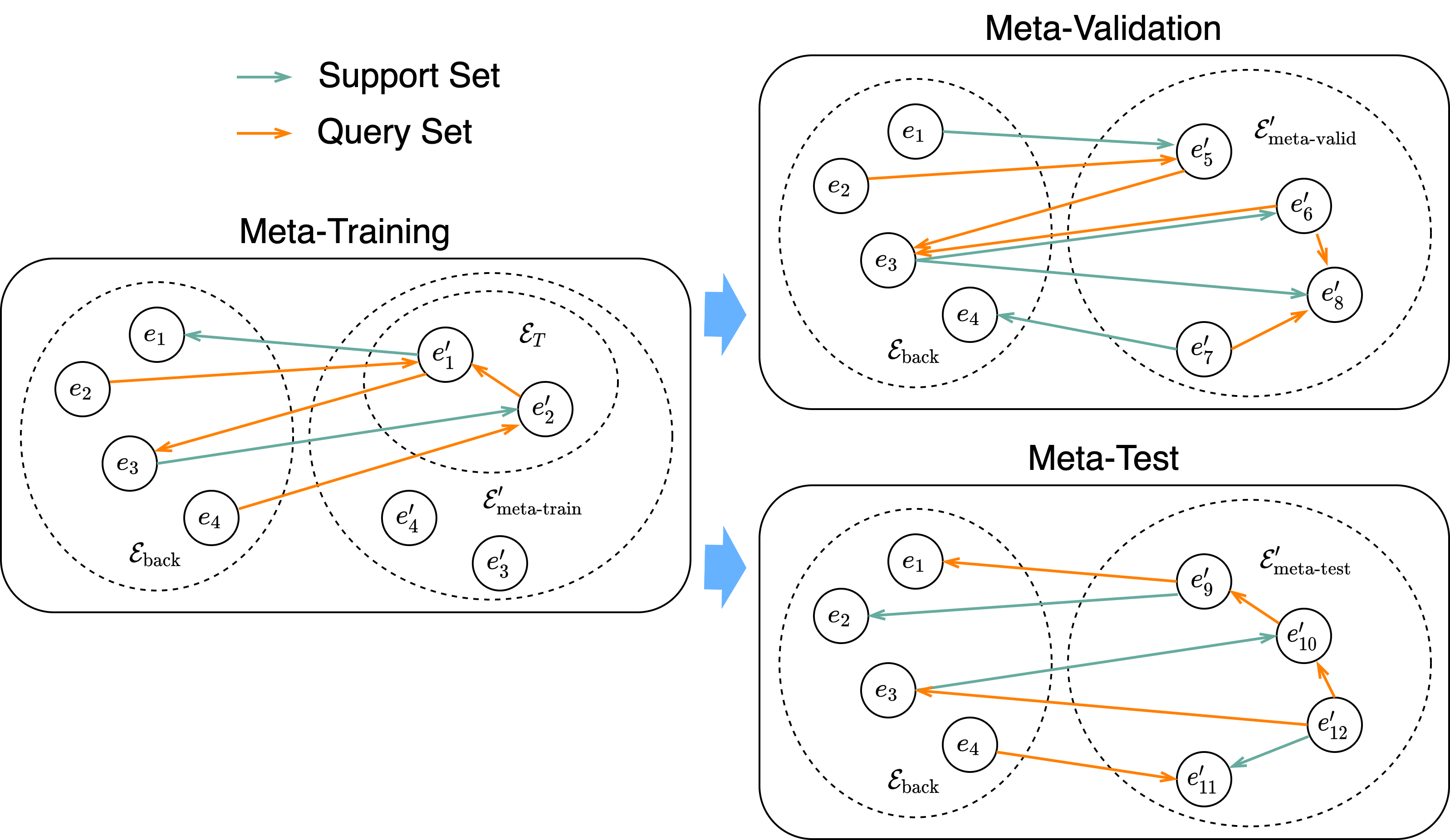
Figure 5: Illustration of the meta-learning framework formulated from the TKG few-shot OOG link prediction task.

TKG few-shot OOG link prediction vs. TKG completion.

For the existing TKGC benchmark datasets, e.g., ICEWS14, there exist a number of entities that only appear in the test sets (or the validation sets) and are unseen in their training sets. Evaluating on the links concerning these unseen entities coincides to the evaluation setting of TKG few-shot OOG link prediction. However, in our proposed task, we focus on the unseen entities that are long-tail, and we also introduce a realistic setting that each unseen entity is coupled with $K$ support quadruples containing itself, while in traditional TKGC benchmark datasets the unseen entities are not guaranteed to be long-tail and no associated edge is given for learning the inductive representations of them. The aim of TKG few-shot OOG link prediction is to ask the TKG reasoning models to learn strong representations of the unseen entities inductively from extracting the information from the provided $K$ support quadruples, which corresponds to the realistic situation where every newly-emerged entity is often coupled with a small number of associated edges.

E Ablation Study Details

We present the detailed equations of graph encoder variants (B1-B3 in Table 3, B4 already presented). In B1, RGCN computes the unseen entity $e^{\prime}$’s representation as:

$$\mathbf{h}_{(e^{\prime},t_{q})}=\frac{1}{|\mathcal{N}_{e^{\prime}}|}\sum_{(\tilde{e}_{i},r_{i},t_{i})\in\mathcal{N}_{e^{\prime}}}\mathbf{W}_{r_{i}}(\mathbf{h}_{\tilde{e}_{i}}),$$ (6)

where $\mathbf{W}_{r_{i}}$ is a weight matrix modeling $r_{i}$. In B2, Time2Vec computes $e^{\prime}$’s representation as:

$$\textbf{h}_{(e^{\prime},t_{q})}=\frac{1}{|\mathcal{N}_{e^{\prime}}|}\sum_{(\tilde{e}_{i},r_{i},t_{i})\in\mathcal{N}_{e^{\prime}}}\textbf{W}_{g}(\textbf{h}_{(\tilde{e}_{i},t_{i})}\|\textbf{h}_{r_{i}}),$$ (7)

where $\textbf{h}_{(\tilde{e}_{i},t_{i})}$ is defined as:

$$\textbf{h}_{(\tilde{e}_{i},t_{i})} =f(\textbf{h}_{\tilde{e}_{i}}\|\Phi(t_{i})),$$ (8)

$$\Phi(t_{i})[j] =\left\{\begin{multlined}\quad\omega_{j}t_{i}+\varphi_{j},\quad\text{if}\ j=0,\\ \sin(\omega_{j}t_{i}+\varphi_{j}),\quad\text{if}\ 1\leq j\leq d_{t}.\end{multlined}\quad\omega_{j}t_{i}+\varphi_{j},\quad\text{if}\ j=0,\\ \sin(\omega_{j}t_{i}+\varphi_{j}),\quad\text{if}\ 1\leq j\leq d_{t}.\right.$$

$f$ denotes a layer of feed forward neural network. $\Phi(t_{i})[j]$ denotes the $j$th component of $t_{i}$’s time representation $\Phi(t_{i})$. $d_{t}$ is the dimension size of time representations. $\omega_{j}$ and $\varphi_{j}$ represent the trainable frequency and phase parameters, respectively. In B3, we use the same aggregation function 7 as in Time2vec, however, we use another form of time encoder to encode time information:

$$\textbf{h}_{(\tilde{e}_{i},t_{i})} =f(\textbf{h}_{\tilde{e}_{i}}\|\Phi(t_{i})),$$ (9)

$$\Phi(t_{i}) =\sqrt{\frac{1}{d_{t}}}[\cos(\omega_{1}t_{i}+\varphi_{1}),\dots,\cos(\omega_{d_{t}}t_{i}+\varphi_{d_{t}}))],$$

where $\omega_{1}\dots\omega_{d_{t}}$ and $\phi_{1}\dots\phi_{d_{t}}$ are trainable parameters.

F Concept Extraction of ICEWS Database

We take the sectors of ICEWS entities as their concepts. The sector classification can be found on the ICEWS official website. ICEWS sectors have hierarchies. We do not consider hierarchies and consider each sector as individual. For example, the sector Foreign Ministry belongs to the sector Government. We learn their representations separately.

A number of entities in the ICEWS coded event data are not labeled with any sector. Some of them are regions, e.g., North Korea. We create a new sector named Region for them. For other entities, we find their affiliations and pick out their sectors. We then choose from their affiliations’ sectors the most suitable ones and label these entities. For example, European Parliament has no associated sector in the ICEWS coded event data. We find its affiliation European Union. European Union is assigned a sector Regional Diplomatic IGOs. We take Regional Diplomatic IGOs as European Parliament’s sector and it is taken as a concept in our meta-learning process.

G Case Study of Learned Concept Representations

We further find three cases to show that our learned concept representations capture the semantic meaning of concepts, which helps to embed unseen entities inductively. We resize the visualization in Figure 3 and label several concepts close to each other.

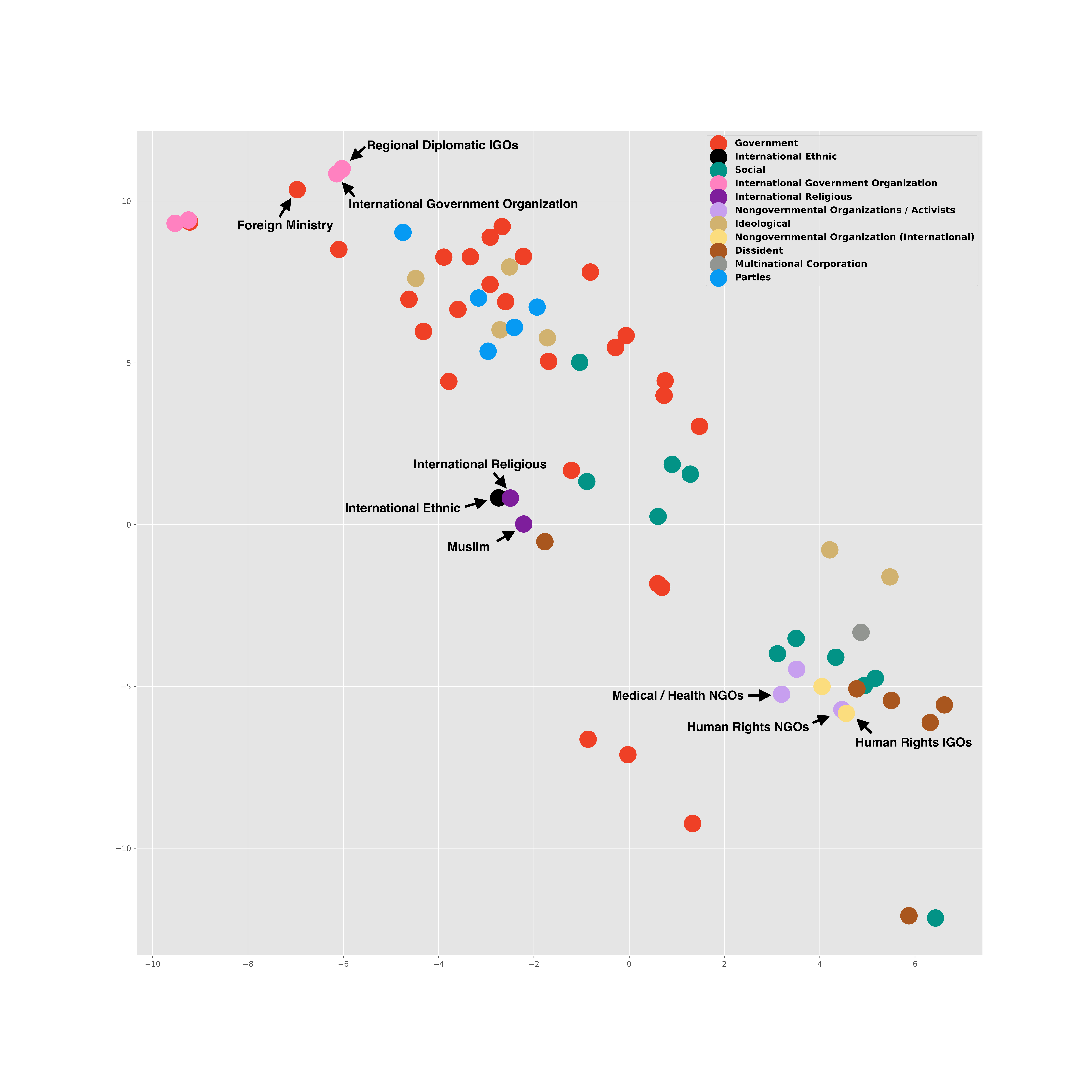
Figure 6: Resized visualization of learned concept representations on 3-shot ICEWS18-OOG.

The first case is about the concepts Foreign Ministry, International Government Organization and Regional Diplomatic IGOs, where IGO stands for international government organization. From human intuition, Foreign Ministry is closely related to international interactions. Similarly, international Government Organization and Regional Diplomatic IGOs also possess the same semantics.

The second case is about the concepts International Ethnic, International Religious and Muslim. Muslim stands for not only a religion but also an ethnicity, therefore, it is close to both International Religious and International Ethnic.

The third case is about the concepts Medical / Health NGOs, Human Rights NGOs and Human Rights IGOs, where NGO stands for nongovernmental organizations. We can observe that Human Rights NGOs and Human Rights IGOs are extremely close to each other. Since protecting human rights is normally concerned with providing medical aid, they are also close to Medical / Health NGOs.

H Dataset Construction Process

• 1. We take ICEWS14, ICEWS18 and ICEWS05-15 as the databases for dataset construction.

• 2. We set the upper and lower thresholds for entity frequencies. We do not want the upper threshold to be large since in real-world scenarios, newly-emerged entities normally are only coupled with very few edges. We also do not want the lower threshold to be too small since we want to include enough test examples. We set the upper and lower threshold to 10 and 25 for every dataset.

• 3. We pick out the entities whose frequencies are between thresholds and sample half of them as the total unseen entities $\mathcal{E}^{\prime}$ (following Baek et al. [2020]). We take the quadruples without any unseen entity as the background graph $\mathcal{G}_{\text{back}}$.

• 4. We split the unseen entities as meta-training $\mathcal{E}^{\prime}_{\text{meta-train}}$, meta-validation $\mathcal{E}^{\prime}_{\text{meta-valid}}$ and meta-test $\mathcal{E}^{\prime}_{\text{meta-test}}$ entities. $|\mathcal{E}^{\prime}_{\text{meta-train}}|:|\mathcal{E}^{\prime}_{\text{meta-valid}}|:|\mathcal{E}^{\prime}_{\text{meta-test}}|\approx 8:1:1$. Their associated quadruples form the corresponding meta-learning sets.

References

- Baek et al. (2020) Jinheon Baek, Dong Bok Lee, and Sung Ju Hwang. Learning to extrapolate knowledge: Transductive few-shot out-of-graph link prediction. In Hugo Larochelle, Marc’Aurelio Ranzato, Raia Hadsell, Maria-Florina Balcan, and Hsuan-Tien Lin, editors, Advances in Neural Information Processing Systems 33: Annual Conference on Neural Information Processing Systems 2020, NeurIPS 2020, December 6-12, 2020, virtual, 2020. URL https://proceedings.neurips.cc/paper/2020/hash/0663a4ddceacb40b095eda264a85f15c-Abstract.html.
- Bordes et al. (2013) Antoine Bordes, Nicolas Usunier, Alberto García-Durán, Jason Weston, and Oksana Yakhnenko. Translating embeddings for modeling multi-relational data. In Christopher J. C. Burges, Léon Bottou, Zoubin Ghahramani, and Kilian Q. Weinberger, editors, Advances in Neural Information Processing Systems 26: 27th Annual Conference on Neural Information Processing Systems 2013. Proceedings of a meeting held December 5-8, 2013, Lake Tahoe, Nevada, United States, pages 2787–2795, 2013. URL https://proceedings.neurips.cc/paper/2013/hash/1cecc7a77928ca8133fa24680a88d2f9-Abstract.html.
- Boschee et al. (2015) Elizabeth Boschee, Jennifer Lautenschlager, Sean O’Brien, Steve Shellman, James Starz, and Michael Ward. ICEWS Coded Event Data, 2015. URL https://doi.org/10.7910/DVN/28075.
- Chen et al. (2019) Mingyang Chen, Wen Zhang, Wei Zhang, Qiang Chen, and Huajun Chen. Meta relational learning for few-shot link prediction in knowledge graphs. In Kentaro Inui, Jing Jiang, Vincent Ng, and Xiaojun Wan, editors, Proceedings of the 2019 Conference on Empirical Methods in Natural Language Processing and the 9th International Joint Conference on Natural Language Processing, EMNLP-IJCNLP 2019, Hong Kong, China, November 3-7, 2019, pages 4216–4225. Association for Computational Linguistics, 2019. doi: 10.18653/v1/D19-1431. URL https://doi.org/10.18653/v1/D19-1431.
- Chen et al. (2018) Tian Qi Chen, Yulia Rubanova, Jesse Bettencourt, and David Duvenaud. Neural ordinary differential equations. In Samy Bengio, Hanna M. Wallach, Hugo Larochelle, Kristen Grauman, Nicolò Cesa-Bianchi, and Roman Garnett, editors, Advances in Neural Information Processing Systems 31: Annual Conference on Neural Information Processing Systems 2018, NeurIPS 2018, December 3-8, 2018, Montréal, Canada, pages 6572–6583, 2018. URL https://proceedings.neurips.cc/paper/2018/hash/69386f6bb1dfed68692a24c8686939b9-Abstract.html.
- Cho et al. (2014) Kyunghyun Cho, Bart van Merrienboer, Çaglar Gülçehre, Dzmitry Bahdanau, Fethi Bougares, Holger Schwenk, and Yoshua Bengio. Learning phrase representations using RNN encoder-decoder for statistical machine translation. In Alessandro Moschitti, Bo Pang, and Walter Daelemans, editors, Proceedings of the 2014 Conference on Empirical Methods in Natural Language Processing, EMNLP 2014, October 25-29, 2014, Doha, Qatar, A meeting of SIGDAT, a Special Interest Group of the ACL, pages 1724–1734. ACL, 2014. doi: 10.3115/v1/d14-1179. URL https://doi.org/10.3115/v1/d14-1179.
- Ding et al. (2021) Zifeng Ding, Yunpu Ma, Bailan He, and Volker Tresp. A simple but powerful graph encoder for temporal knowledge graph completion. CoRR, abs/2112.07791, 2021. URL https://arxiv.org/abs/2112.07791.
- Ding et al. (2022a) Zifeng Ding, Bailan He, Yunpu Ma, Zhen Han, and Volker Tresp. Learning meta representations of one-shot relations for temporal knowledge graph link prediction. CoRR, abs/2205.10621, 2022a. doi: 10.48550/arXiv.2205.10621. URL https://doi.org/10.48550/arXiv.2205.10621.
- Ding et al. (2022b) Zifeng Ding, Ruoxia Qi, Zongyue Li, Bailan He, Jingpei Wu, Yunpu Ma, Zhao Meng, Zhen Han, and Volker Tresp. Forecasting question answering over temporal knowledge graphs. CoRR, abs/2208.06501, 2022b. doi: 10.48550/arXiv.2208.06501. URL https://doi.org/10.48550/arXiv.2208.06501.
- Guo and Kok (2021) Jia Guo and Stanley Kok. Bique: Biquaternionic embeddings of knowledge graphs. In Marie-Francine Moens, Xuanjing Huang, Lucia Specia, and Scott Wen-tau Yih, editors, Proceedings of the 2021 Conference on Empirical Methods in Natural Language Processing, EMNLP 2021, Virtual Event / Punta Cana, Dominican Republic, 7-11 November, 2021, pages 8338–8351. Association for Computational Linguistics, 2021. doi: 10.18653/v1/2021.emnlp-main.657. URL https://doi.org/10.18653/v1/2021.emnlp-main.657.
- Hamaguchi et al. (2017) Takuo Hamaguchi, Hidekazu Oiwa, Masashi Shimbo, and Yuji Matsumoto. Knowledge transfer for out-of-knowledge-base entities : A graph neural network approach. In Carles Sierra, editor, Proceedings of the Twenty-Sixth International Joint Conference on Artificial Intelligence, IJCAI 2017, Melbourne, Australia, August 19-25, 2017, pages 1802–1808. ijcai.org, 2017. doi: 10.24963/ijcai.2017/250. URL https://doi.org/10.24963/ijcai.2017/250.
- Han et al. (2020a) Zhen Han, Yunpu Ma, Peng Chen, and Volker Tresp. Dyernie: Dynamic evolution of riemannian manifold embeddings for temporal knowledge graph completion. arXiv preprint arXiv:2011.03984, 2020a.
- Han et al. (2020b) Zhen Han, Yunpu Ma, Yuyi Wang, Stephan Günnemann, and Volker Tresp. Graph hawkes neural network for forecasting on temporal knowledge graphs. arXiv preprint arXiv:2003.13432, 2020b.
- Han et al. (2021a) Zhen Han, Peng Chen, Yunpu Ma, and Volker Tresp. Explainable subgraph reasoning for forecasting on temporal knowledge graphs. In 9th International Conference on Learning Representations, ICLR 2021, Virtual Event, Austria, May 3-7, 2021. OpenReview.net, 2021a. URL https://openreview.net/forum?id=pGIHq1m7PU.
- Han et al. (2021b) Zhen Han, Zifeng Ding, Yunpu Ma, Yujia Gu, and Volker Tresp. Learning neural ordinary equations for forecasting future links on temporal knowledge graphs. In Marie-Francine Moens, Xuanjing Huang, Lucia Specia, and Scott Wen-tau Yih, editors, Proceedings of the 2021 Conference on Empirical Methods in Natural Language Processing, EMNLP 2021, Virtual Event / Punta Cana, Dominican Republic, 7-11 November, 2021, pages 8352–8364. Association for Computational Linguistics, 2021b. doi: 10.18653/v1/2021.emnlp-main.658. URL https://doi.org/10.18653/v1/2021.emnlp-main.658.
- Han et al. (2021c) Zhen Han, Gengyuan Zhang, Yunpu Ma, and Volker Tresp. Time-dependent entity embedding is not all you need: A re-evaluation of temporal knowledge graph completion models under a unified framework. In Proceedings of the 2021 Conference on Empirical Methods in Natural Language Processing, pages 8104–8118, Online and Punta Cana, Dominican Republic, November 2021c. Association for Computational Linguistics. doi: 10.18653/v1/2021.emnlp-main.639. URL https://aclanthology.org/2021.emnlp-main.639.
- He et al. (2020) Yongquan He, Zhihan Wang, Peng Zhang, Zhaopeng Tu, and Zhaochun Ren. VN network: Embedding newly emerging entities with virtual neighbors. In Mathieu d’Aquin, Stefan Dietze, Claudia Hauff, Edward Curry, and Philippe Cudré-Mauroux, editors, CIKM ’20: The 29th ACM International Conference on Information and Knowledge Management, Virtual Event, Ireland, October 19-23, 2020, pages 505–514. ACM, 2020. doi: 10.1145/3340531.3411865. URL https://doi.org/10.1145/3340531.3411865.
- Jung et al. (2021) Jaehun Jung, Jinhong Jung, and U Kang. Learning to walk across time for interpretable temporal knowledge graph completion. In Feida Zhu, Beng Chin Ooi, and Chunyan Miao, editors, KDD ’21: The 27th ACM SIGKDD Conference on Knowledge Discovery and Data Mining, Virtual Event, Singapore, August 14-18, 2021, pages 786–795. ACM, 2021. doi: 10.1145/3447548.3467292. URL https://doi.org/10.1145/3447548.3467292.
- Kazemi et al. (2019) Seyed Mehran Kazemi, Rishab Goel, Sepehr Eghbali, Janahan Ramanan, Jaspreet Sahota, Sanjay Thakur, Stella Wu, Cathal Smyth, Pascal Poupart, and Marcus A. Brubaker. Time2vec: Learning a vector representation of time. CoRR, abs/1907.05321, 2019. URL http://arxiv.org/abs/1907.05321.
- Lacroix et al. (2020) Timothée Lacroix, Guillaume Obozinski, and Nicolas Usunier. Tensor decompositions for temporal knowledge base completion. In 8th International Conference on Learning Representations, ICLR 2020, Addis Ababa, Ethiopia, April 26-30, 2020. OpenReview.net, 2020. URL https://openreview.net/forum?id=rke2P1BFwS.
- Leblay and Chekol (2018) Julien Leblay and Melisachew Wudage Chekol. Deriving validity time in knowledge graph. In Pierre-Antoine Champin, Fabien Gandon, Mounia Lalmas, and Panagiotis G. Ipeirotis, editors, Companion of the The Web Conference 2018 on The Web Conference 2018, WWW 2018, Lyon , France, April 23-27, 2018, pages 1771–1776. ACM, 2018. doi: 10.1145/3184558.3191639. URL https://doi.org/10.1145/3184558.3191639.
- Li et al. (2020) Wei Li, Ruihan Bao, Keiko Harimoto, Deli Chen, Jingjing Xu, and Qi Su. Modeling the stock relation with graph network for overnight stock movement prediction. In Christian Bessiere, editor, Proceedings of the Twenty-Ninth International Joint Conference on Artificial Intelligence, IJCAI 2020, pages 4541–4547. ijcai.org, 2020. doi: 10.24963/ijcai.2020/626. URL https://doi.org/10.24963/ijcai.2020/626.
- Ma et al. (2019) Yunpu Ma, Volker Tresp, and Erik A. Daxberger. Embedding models for episodic knowledge graphs. J. Web Semant., 59, 2019.
- Min et al. (2013) Bonan Min, Ralph Grishman, Li Wan, Chang Wang, and David Gondek. Distant supervision for relation extraction with an incomplete knowledge base. In Lucy Vanderwende, Hal Daumé III, and Katrin Kirchhoff, editors, Human Language Technologies: Conference of the North American Chapter of the Association of Computational Linguistics, Proceedings, June 9-14, 2013, Westin Peachtree Plaza Hotel, Atlanta, Georgia, USA, pages 777–782. The Association for Computational Linguistics, 2013. URL https://aclanthology.org/N13-1095/.
- Mirtaheri et al. (2021) Mehrnoosh Mirtaheri, Mohammad Rostami, Xiang Ren, Fred Morstatter, and Aram Galstyan. One-shot learning for temporal knowledge graphs. In 3rd Conference on Automated Knowledge Base Construction, 2021.
- Nickel et al. (2011) Maximilian Nickel, Volker Tresp, and Hans-Peter Kriegel. A three-way model for collective learning on multi-relational data. In Lise Getoor and Tobias Scheffer, editors, Proceedings of the 28th International Conference on Machine Learning, ICML 2011, Bellevue, Washington, USA, June 28 - July 2, 2011, pages 809–816. Omnipress, 2011. URL https://icml.cc/2011/papers/438_icmlpaper.pdf.
- Paszke et al. (2019) Adam Paszke, Sam Gross, Francisco Massa, Adam Lerer, James Bradbury, Gregory Chanan, Trevor Killeen, Zeming Lin, Natalia Gimelshein, Luca Antiga, Alban Desmaison, Andreas Köpf, Edward Z. Yang, Zachary DeVito, Martin Raison, Alykhan Tejani, Sasank Chilamkurthy, Benoit Steiner, Lu Fang, Junjie Bai, and Soumith Chintala. Pytorch: An imperative style, high-performance deep learning library. In Hanna M. Wallach, Hugo Larochelle, Alina Beygelzimer, Florence d’Alché-Buc, Emily B. Fox, and Roman Garnett, editors, Advances in Neural Information Processing Systems 32: Annual Conference on Neural Information Processing Systems 2019, NeurIPS 2019, December 8-14, 2019, Vancouver, BC, Canada, pages 8024–8035, 2019. URL https://proceedings.neurips.cc/paper/2019/hash/bdbca288fee7f92f2bfa9f7012727740-Abstract.html.
- Sadeghian et al. (2021) Ali Sadeghian, Mohammadreza Armandpour, Anthony Colas, and Daisy Zhe Wang. Chronor: Rotation based temporal knowledge graph embedding. In Thirty-Fifth AAAI Conference on Artificial Intelligence, AAAI 2021, Thirty-Third Conference on Innovative Applications of Artificial Intelligence, IAAI 2021, The Eleventh Symposium on Educational Advances in Artificial Intelligence, EAAI 2021, Virtual Event, February 2-9, 2021, pages 6471–6479. AAAI Press, 2021. URL https://ojs.aaai.org/index.php/AAAI/article/view/16802.
- Saxena et al. (2020) Apoorv Saxena, Aditay Tripathi, and Partha Talukdar. Improving multi-hop question answering over knowledge graphs using knowledge base embeddings. In Proceedings of the 58th Annual Meeting of the Association for Computational Linguistics, pages 4498–4507, Online, July 2020. Association for Computational Linguistics. doi: 10.18653/v1/2020.acl-main.412. URL https://aclanthology.org/2020.acl-main.412.
- Schlichtkrull et al. (2018) Michael Sejr Schlichtkrull, Thomas N. Kipf, Peter Bloem, Rianne van den Berg, Ivan Titov, and Max Welling. Modeling relational data with graph convolutional networks. In Aldo Gangemi, Roberto Navigli, Maria-Esther Vidal, Pascal Hitzler, Raphaël Troncy, Laura Hollink, Anna Tordai, and Mehwish Alam, editors, The Semantic Web - 15th International Conference, ESWC 2018, Heraklion, Crete, Greece, June 3-7, 2018, Proceedings, volume 10843 of Lecture Notes in Computer Science, pages 593–607. Springer, 2018. doi: 10.1007/978-3-319-93417-4“˙38. URL https://doi.org/10.1007/978-3-319-93417-4_38.
- Sheng et al. (2020) Jiawei Sheng, Shu Guo, Zhenyu Chen, Juwei Yue, Lihong Wang, Tingwen Liu, and Hongbo Xu. Adaptive attentional network for few-shot knowledge graph completion. In Bonnie Webber, Trevor Cohn, Yulan He, and Yang Liu, editors, Proceedings of the 2020 Conference on Empirical Methods in Natural Language Processing, EMNLP 2020, Online, November 16-20, 2020, pages 1681–1691. Association for Computational Linguistics, 2020. doi: 10.18653/v1/2020.emnlp-main.131. URL https://doi.org/10.18653/v1/2020.emnlp-main.131.
- Shi and Weninger (2018) Baoxu Shi and Tim Weninger. Open-world knowledge graph completion. In Sheila A. McIlraith and Kilian Q. Weinberger, editors, Proceedings of the Thirty-Second AAAI Conference on Artificial Intelligence, (AAAI-18), the 30th innovative Applications of Artificial Intelligence (IAAI-18), and the 8th AAAI Symposium on Educational Advances in Artificial Intelligence (EAAI-18), New Orleans, Louisiana, USA, February 2-7, 2018, pages 1957–1964. AAAI Press, 2018. URL https://www.aaai.org/ocs/index.php/AAAI/AAAI18/paper/view/16055.
- Sun et al. (2021) Haohai Sun, Jialun Zhong, Yunpu Ma, Zhen Han, and Kun He. TimeTraveler: Reinforcement learning for temporal knowledge graph forecasting. In Proceedings of the 2021 Conference on Empirical Methods in Natural Language Processing, pages 8306–8319, Online and Punta Cana, Dominican Republic, November 2021. Association for Computational Linguistics. doi: 10.18653/v1/2021.emnlp-main.655. URL https://aclanthology.org/2021.emnlp-main.655.
- Sun et al. (2019) Zhiqing Sun, Zhi-Hong Deng, Jian-Yun Nie, and Jian Tang. Rotate: Knowledge graph embedding by relational rotation in complex space. In 7th International Conference on Learning Representations, ICLR 2019, New Orleans, LA, USA, May 6-9, 2019. OpenReview.net, 2019. URL https://openreview.net/forum?id=HkgEQnRqYQ.
- Tresp et al. (2015) Volker Tresp, Cristóbal Esteban, Yinchong Yang, Stephan Baier, and Denis Krompaß. Learning with memory embeddings. arXiv preprint arXiv:1511.07972, 2015.
- Trouillon et al. (2016) Théo Trouillon, Johannes Welbl, Sebastian Riedel, Éric Gaussier, and Guillaume Bouchard. Complex embeddings for simple link prediction. In Maria-Florina Balcan and Kilian Q. Weinberger, editors, Proceedings of the 33nd International Conference on Machine Learning, ICML 2016, New York City, NY, USA, June 19-24, 2016, volume 48 of JMLR Workshop and Conference Proceedings, pages 2071–2080. JMLR.org, 2016. URL http://proceedings.mlr.press/v48/trouillon16.html.
- Van der Maaten and Hinton (2008) Laurens Van der Maaten and Geoffrey Hinton. Visualizing data using t-sne. Journal of machine learning research, 9(11), 2008.
- Vashishth et al. (2020) Shikhar Vashishth, Soumya Sanyal, Vikram Nitin, and Partha P. Talukdar. Composition-based multi-relational graph convolutional networks. In 8th International Conference on Learning Representations, ICLR 2020, Addis Ababa, Ethiopia, April 26-30, 2020. OpenReview.net, 2020. URL https://openreview.net/forum?id=BylA_C4tPr.
- Wang et al. (2019a) Hongwei Wang, Miao Zhao, Xing Xie, Wenjie Li, and Minyi Guo. Knowledge graph convolutional networks for recommender systems. In Ling Liu, Ryen W. White, Amin Mantrach, Fabrizio Silvestri, Julian J. McAuley, Ricardo Baeza-Yates, and Leila Zia, editors, The World Wide Web Conference, WWW 2019, San Francisco, CA, USA, May 13-17, 2019, pages 3307–3313. ACM, 2019a. doi: 10.1145/3308558.3313417. URL https://doi.org/10.1145/3308558.3313417.
- Wang et al. (2019b) Peifeng Wang, Jialong Han, Chenliang Li, and Rong Pan. Logic attention based neighborhood aggregation for inductive knowledge graph embedding. In The Thirty-Third AAAI Conference on Artificial Intelligence, AAAI 2019, The Thirty-First Innovative Applications of Artificial Intelligence Conference, IAAI 2019, The Ninth AAAI Symposium on Educational Advances in Artificial Intelligence, EAAI 2019, Honolulu, Hawaii, USA, January 27 - February 1, 2019, pages 7152–7159. AAAI Press, 2019b. doi: 10.1609/aaai.v33i01.33017152. URL https://doi.org/10.1609/aaai.v33i01.33017152.
- Wang et al. (2019c) Xiang Wang, Dingxian Wang, Canran Xu, Xiangnan He, Yixin Cao, and Tat-Seng Chua. Explainable reasoning over knowledge graphs for recommendation. In The Thirty-Third AAAI Conference on Artificial Intelligence, AAAI 2019, The Thirty-First Innovative Applications of Artificial Intelligence Conference, IAAI 2019, The Ninth AAAI Symposium on Educational Advances in Artificial Intelligence, EAAI 2019, Honolulu, Hawaii, USA, January 27 - February 1, 2019, pages 5329–5336. AAAI Press, 2019c. doi: 10.1609/aaai.v33i01.33015329. URL https://doi.org/10.1609/aaai.v33i01.33015329.
- Wang et al. (2019d) Zihao Wang, Kwun Ping Lai, Piji Li, Lidong Bing, and Wai Lam. Tackling long-tailed relations and uncommon entities in knowledge graph completion. In Kentaro Inui, Jing Jiang, Vincent Ng, and Xiaojun Wan, editors, Proceedings of the 2019 Conference on Empirical Methods in Natural Language Processing and the 9th International Joint Conference on Natural Language Processing, EMNLP-IJCNLP 2019, Hong Kong, China, November 3-7, 2019, pages 250–260. Association for Computational Linguistics, 2019d. doi: 10.18653/v1/D19-1024. URL https://doi.org/10.18653/v1/D19-1024.
- Wu et al. (2020) Jiapeng Wu, Meng Cao, Jackie Chi Kit Cheung, and William L. Hamilton. Temp: Temporal message passing for temporal knowledge graph completion. In Bonnie Webber, Trevor Cohn, Yulan He, and Yang Liu, editors, Proceedings of the 2020 Conference on Empirical Methods in Natural Language Processing, EMNLP 2020, Online, November 16-20, 2020, pages 5730–5746. Association for Computational Linguistics, 2020. doi: 10.18653/v1/2020.emnlp-main.462. URL https://doi.org/10.18653/v1/2020.emnlp-main.462.
- Xie et al. (2016) Ruobing Xie, Zhiyuan Liu, Jia Jia, Huanbo Luan, and Maosong Sun. Representation learning of knowledge graphs with entity descriptions. In Dale Schuurmans and Michael P. Wellman, editors, Proceedings of the Thirtieth AAAI Conference on Artificial Intelligence, February 12-17, 2016, Phoenix, Arizona, USA, pages 2659–2665. AAAI Press, 2016. URL http://www.aaai.org/ocs/index.php/AAAI/AAAI16/paper/view/12216.
- Xiong et al. (2018) Wenhan Xiong, Mo Yu, Shiyu Chang, Xiaoxiao Guo, and William Yang Wang. One-shot relational learning for knowledge graphs. In Ellen Riloff, David Chiang, Julia Hockenmaier, and Jun’ichi Tsujii, editors, Proceedings of the 2018 Conference on Empirical Methods in Natural Language Processing, Brussels, Belgium, October 31 - November 4, 2018, pages 1980–1990. Association for Computational Linguistics, 2018. doi: 10.18653/v1/d18-1223. URL https://doi.org/10.18653/v1/d18-1223.
- Xu et al. (2020a) Chengjin Xu, Mojtaba Nayyeri, Fouad Alkhoury, Hamed Shariat Yazdi, and Jens Lehmann. Tero: A time-aware knowledge graph embedding via temporal rotation. In Donia Scott, Núria Bel, and Chengqing Zong, editors, Proceedings of the 28th International Conference on Computational Linguistics, COLING 2020, Barcelona, Spain (Online), December 8-13, 2020, pages 1583–1593. International Committee on Computational Linguistics, 2020a. doi: 10.18653/v1/2020.coling-main.139. URL https://doi.org/10.18653/v1/2020.coling-main.139.
- Xu et al. (2021a) Chengjin Xu, Yung-Yu Chen, Mojtaba Nayyeri, and Jens Lehmann. Temporal knowledge graph completion using a linear temporal regularizer and multivector embeddings. In Kristina Toutanova, Anna Rumshisky, Luke Zettlemoyer, Dilek Hakkani-Tür, Iz Beltagy, Steven Bethard, Ryan Cotterell, Tanmoy Chakraborty, and Yichao Zhou, editors, Proceedings of the 2021 Conference of the North American Chapter of the Association for Computational Linguistics: Human Language Technologies, NAACL-HLT 2021, Online, June 6-11, 2021, pages 2569–2578. Association for Computational Linguistics, 2021a. doi: 10.18653/v1/2021.naacl-main.202. URL https://doi.org/10.18653/v1/2021.naacl-main.202.
- Xu et al. (2020b) Da Xu, Chuanwei Ruan, Evren Körpeoglu, Sushant Kumar, and Kannan Achan. Inductive representation learning on temporal graphs. In 8th International Conference on Learning Representations, ICLR 2020, Addis Ababa, Ethiopia, April 26-30, 2020. OpenReview.net, 2020b. URL https://openreview.net/forum?id=rJeW1yHYwH.
- Xu et al. (2021b) Wentao Xu, Weiqing Liu, Lewen Wang, Yingce Xia, Jiang Bian, Jian Yin, and Tie-Yan Liu. HIST: A graph-based framework for stock trend forecasting via mining concept-oriented shared information. CoRR, abs/2110.13716, 2021b. URL https://arxiv.org/abs/2110.13716.
- Yu et al. (2021) Donghan Yu, Yiming Yang, Ruohong Zhang, and Yuexin Wu. Knowledge embedding based graph convolutional network. In Jure Leskovec, Marko Grobelnik, Marc Najork, Jie Tang, and Leila Zia, editors, WWW ’21: The Web Conference 2021, Virtual Event / Ljubljana, Slovenia, April 19-23, 2021, pages 1619–1628. ACM / IW3C2, 2021. doi: 10.1145/3442381.3449925. URL https://doi.org/10.1145/3442381.3449925.
- Zhang et al. (2021) Yufeng Zhang, Weiqing Wang, Wei Chen, Jiajie Xu, An Liu, and Lei Zhao. Meta-learning based hyper-relation feature modeling for out-of-knowledge-base embedding. In Gianluca Demartini, Guido Zuccon, J. Shane Culpepper, Zi Huang, and Hanghang Tong, editors, CIKM ’21: The 30th ACM International Conference on Information and Knowledge Management, Virtual Event, Queensland, Australia, November 1 - 5, 2021, pages 2637–2646. ACM, 2021. doi: 10.1145/3459637.3482367. URL https://doi.org/10.1145/3459637.3482367.