The inflationary scenario in the $f(R)$ gravity model with a $R^{4}$ term

Abstract

Abstract

We investigate the cosmic inflation scenario of a specific $f(R)$ model that contains more than one higher-order term in $R$. The $f(R)$ considered here has the terms $R^{2}$, $R^{3}$, and $R^{4}$ along with the linear term. A rigorous investigation has been carried out in the presence of these higher-order terms to figure out whether it leads to a physically sensible cosmic inflationary model. We examine in detail, subject to which conditions this $f(R)$ model renders a viable inflationary scenario, and it has been found that the outcomes of our study agree well with the recent PLANCK results.

I Introduction

There has been a huge interest in the study of cosmic inflation over the decades since it is considered as an effective scenario for explaining the origin of structure formation of the Universe. There has been a huge interest in the study of cosmic inflation over the decades since it is considered as an effective scenario for explaining the origin of structure formation of the Universe. In the article [1], Starobinsky showed that Einstein’s equations with quantum one-loop contributions of conformally covariant matter fields admit a class of nonsingular isotropic homogeneous solutions that correspond to a picture of the Universe and it attracted a huge attentions since successful slow-roll inflation can be achieved with a single parameter which is the coefficient of the $R^{2}$ curvature term. The predictions related to inflation of this model are well consistent with the Planck data. Therefore, the discussion has been generalized to a class of Starobinsky-like models having common properties during inflation [2, 3, 4, 5, 6, 7]. The Higgs inflation as a particular case was studied in [8]. In the article [4], it has been emphasized that there must be a stage of inflation in the early Universe to have a consistent cosmological picture.The articles [9, 10, 11] contain the studies of different aspects of Starobinsky and Starobinsky-like models. The Starobonsky model was extended with the higher-order term in $R$ in the articles [12, 13, 14]. Although the $\Lambda$$CDM$ model provides a consistent explanation for the accelerating expansion of the universe, the formation of large scale structure, cold dark matter, and even for the most mysterious dark energy, it still suffers from the horizon, flatness, homogeneity, and so-called magnetic monopole problems. The elegant introduction of inflation scenario eradicates these problems in a fascinating way [1, 15, 16], and the study of the cosmological observations on the cosmic microwave background anisotropy have confirmed the predictions of inflation quite a long ago with a good degree of accuracy. The most common framework for inflation is based on a scalar field [17, 18] that dominates the energy density of the universe and rolls down slowly following an almost flat potential $V(\phi)$. At the end of inflation, the scalar field decays and the known environments for the standard hot big-bang cosmology evolves out. This hypothetical scalar field remains mysterious and to construct an inflationary scenario, we need either an extension of the standard model of particle physics or alternatively, this scalar degree of freedom can be thought of as its origin lies in the gravitational sector. The theory that includes a scalar field is the well known Brans-Dicke theory. For the vanishing Brans-Dicke parameter, this theory dynamically corresponds to $f(R)$ gravity theory, where $f(R)$ is a general function of the Ricci scalar [19, 20]. A conformal transformation makes this theory equivalent to Einstein’s theory of gravity which has minimal coupling to a scalar field with a canonical kinetic term and a specific potential described in terms of the function $f(R)$. Whether this scalar field, with a gravitational origin, can act as an inflation field that depends on the imposition of constraints on function $f(R)$ such that it can offer a viable form of the potentials. In this context, the slow-rolling conditions on $V(\phi)$ plays a crucial role.

The Starobinsky inflation model [1] attracted huge attention in this respect because successful slow-roll inflation can be obtained with a single parameter beyond the standard cosmological model, namely the coefficient of the $R^{2}$ term. The inflationary predictions of the Starobinsky model are in excellent concordance with the recent CMB anisotropy data [21, 22, 23, *chowdhury2019assessing] as well. Therefore, extension, as well as a generalization, been made to a class of Starobinsky-like models with common properties during inflation [1, 3, 4, 5, 6, 7, 9, 10, 11, 12, 13, 14], including Higgs inflation as a particular case [8, 25]. Together with this framework, inflation can also, be generated in higher dimensional theory through the compactification of extra dimensions [26, 27, 28].

Extension of inflationary models with different $f(R)$ has been reported after the pioneering work of Starobinsky [1]. A logarithmic $f(R)$ has been used in the article [29]. An inflationary model with $f(r)$ having the form $R^{2}+R^{n}$ is discussed elaborately in [30]. In the article [31], $f(R)=R+R^{4}$ is taken to construct an inflationary model. So the studies of formulation of the inflationary model with different choices of $f(R)$ and the necessary constraints on the free parameter used in the models have been enriching this field over the years. It should be mentioned that these higher order terms of curvature scalar $R$ start contributing if the spacetime curvature is very high, which was expected to be in the very early universe, i.e. in the vicinity of the Planck energy. The physics of this high energy/curvature might be completely understood under the framework of a string theory-like or supergravity-type UV completing quantum gravity theory [30]. On the other hand, origin of these higher order terms can also be realized from the perspective of compactification of extra spatial dimensions of higher dimensional theories, where the quartic term in $R$ is naturally favored [32]. In this sense the study of inflationary scenario with $R^{4}$ term is of worth investigation.

Starobnisky model was extended with $R^{4}$ term in [ketov2011embeddin] and it was shown that it led to successful slow roll. In [33] an extension of the Starobnisky model has been made with with $R^{3}$ term and it has been established that it leads to a successful inflationary model. Here we are intended deal with a generalized extension considering the presence of both the $R^{3}$ and $R^{4}$ term. The addition of higher order term although invites computational difficulty however it would be of worth investigation whether with the presence of both $R^{3}$ and $R^{4}$ is capable of leading to a successful inflationary model. Whether the presence of $R^{3}$ term along with $R^{4}$ spoil the slow roll is also a matter of investigation. In this article, an attempt, is therefore, made to formulate an inflationary model with this specific $f(R)$ and carry out a detail investigation towards constraining the free parameters in order to make it a physically sensible framework for cosmic inflation. We analyze inflation in both the original and Einstein frames emphasizing that the scalar field picture is essential to study the detailed consequences of inflation like the number of e-folds, spectral index, tensor-to-scalar ratio and reheating after inflation.

The article is organized as follows. In Sec. II a general discussion of inflationary model based on $f(R)$ gravity is given. Sec.III. is devoted to the description of an inflationary model containing both $R^{3}$ and $R^{4}$ term with the evaluation of the potential. Sec.IV contains a discussion on constraining the free parameters to make an agreement with the available experimental data in order to make the model physically sensible with the evaluation of the slow-roll parameters, the number of e-folds, tensor to scalar ratio and the scalar spectral index. A discussion on the nature of potential is also presented in this section. In Sec.V, an estimation of the mass of the scalar field, the maximum reheating temperature and numbers of e-folds is made. In section VI, a comparison of the results of the models constituted with three different $f(R)$ has been made to establish that the higher order term renders result with better precision because of the freedom offered by extra free parameter. Finally, A brief summary of the work and a general discussion is given in Sec.VII.

II Inflationary model based on $f(R)$ gravity

The general $f(R)$ theory of gravity, in a system of units where the reduced Planck mass ${M_{Pl}}\equiv{(8\pi G_{N})^{-1/2}}=1$, is defined by the action

$$S=\frac{1}{2}\int d^{4}x\sqrt{-g}f(R)+\int d^{4}x{\cal L}(g_{\mu\nu},\psi),$$ (1)

where $f(R)=R+\tilde{f}(R)$. The determinant of the metric $g_{\mu\nu}$ is represented by $g$, $R_{\mu\nu}$ is the well known Ricci tensor and $R=g_{\mu\nu}R^{\mu\nu}$. The field $\psi_{m}$ represents the matter field. The field equation is obtained varying the action (1):

$$f^{\prime}R_{\mu\nu}-\frac{1}{2}g_{\mu\nu}+(g_{\mu\nu}\Box-\nabla_{\mu}\nabla_{\nu})f^{\prime}=T_{\mu\nu},$$ (2)

where $f^{\prime}=\frac{df}{dR}$ and the energy momentum tensor $T_{\mu\nu}=\frac{1}{\sqrt{-g}}\frac{\partial{\cal L}}{\partial g^{\mu\nu}}$. Trace of the field equation (2) leads to

$$3\Box f^{\prime}+f^{\prime}R-2f=T$$ (3)

Where $T$ = $g^{\mu\nu}T_{\mu\nu}$. This modified gravity contains a scalar degrees of freedom which gets manifested when a conformal transformation decouples it from metric to scalar field. The conformal transformation leads to

$$S=\frac{1}{2}\int d^{4}x\sqrt{g}[f(\phi)+f^{\prime}(\phi)(R-\phi)$$ (4)

Defining $\Phi=f^{\prime}(\phi)$, and assuming the invertibility of the relation this action can be written with a scalar field having minimal coupling with gravity as follows

$$S=\int d^{4}x\sqrt{-g}[\frac{1}{2}\phi R-U(\Phi)],$$ (5)

where the potential is given by

$$U(\Phi)=\frac{(\Phi-1)\chi(\phi)-\tilde{f}\chi(\Phi)}{2},$$ (6)

and frame function reads

$$\Phi\equiv 1+\frac{\partial}{{\partial\chi}}[\tilde{f}(\chi)].$$ (7)

The action in the Einstein frame can be obtained by the conformal transformation $g^{\mu\nu}_{E}=\Phi g^{\mu\nu}$ which leads to

$$S=\int d^{4}x\sqrt{-g_{E}}[\frac{1}{2}\phi R_{E}-\frac{1}{2}g_{E}^{\mu\nu}-V(\phi)],$$ (8)

where $V(\phi)$ has the expression

$$V(\phi)=\frac{1}{2\Phi^{2}}[(\Phi-1)\chi(\Phi)-\tilde{f}\chi(\phi)],$$ (9)

and $\Phi$ and $\phi$ are related by the expression

$$\Phi=e^{\sqrt{\frac{2}{3}}\phi}.$$ (10)

Hereafter we will use Einstein frame for computation however we will omit the subscript ’E’ for convenience. The slow-roll parameters $\epsilon$ and $\eta$ that follows from the action (8) respectively defined by [34, *liddle1994formalizing]

$$\epsilon=\frac{1}{2}{\left({\frac{{{V}^{\prime}}}{{{V}}}}\right)^{2}},$$ (11)

$$\eta=\frac{{{V}^{\prime\prime}}}{{{V}}}.$$ (12)

Here the symbol prime (^′) denotes derivative with respect to $\phi$. In this framework the amplitude of primordial scalar power spectrum is defined by [34, *liddle1994formalizing, 17, 18]

$$\Delta^{2}_{R}=\frac{1}{24\pi^{2}}\frac{V}{\epsilon}.$$ (13)

The number of times the universe expands during inflation to acquire the value $\phi_{end}$ starting from the value $\phi_{N}$ is known as the e-fold number which is known to have the expression [34, *liddle1994formalizing, 17, 18]

$$N\equiv\ln\frac{{{a_{end}}}}{{{a_{N}}}}=\int_{{t_{N}}}^{{t_{end}}}Hdt\simeq\int_{{\phi_{end}}}^{{\phi_{N}}}{\frac{V}{{V^{\prime}}}}\,d\phi.$$ (14)

Here $a$ is the scale factor and $H$ represents the Hubble parameter. For this type of inflationary model there exist standard expression of scalar spectral index or scalar tilt $n_{s}$ and the tensor-to-scalar ratio $r$ with the slow-roll parameter $\epsilon$ and $\eta$ [34, *liddle1994formalizing]:

$$n_{s}=1-6\epsilon+2\eta,$$ (15)

$$r=16\epsilon.$$ (16)

This is in short a of general discussion over $F(R)$ inflationary model. What follows next is the formulation of a new inflationary model with this input.

III Inflationary model with a $f(R)$ containing both the $R^{3}$ and $R^{4}$ terms

In this article, an attempt has been made to formulate an inflationary model where $f(R)$ contains both the $R^{3}$ and $R^{4}$ term along with the term $R^{2}$. The model with only $R^{3}$ term is studied in detail in [33]. Our work, in fact, is an extension over the model studied in [33] to investigate whether both the presence of $R^{3}$ and $R^{4}$ terms in the action can offer a successful inflation scenario. To this end, we consider

$$f(R)=R+\frac{R^{2}}{6M^{2}}+\sum_{n=3,4}\frac{\lambda_{n}}{2n}\frac{R^{n}}{(3M^{2})^{n}},$$ (17)

where $M$ is the mass scale or energy scale of the theory and $\lambda$’s are the dimensionless coupling constants whose numerical values ${\lambda_{3,4}}\ll 1$, in order to evade the quantum gravity effects at the energy scale of inflation. It will be handy for computation if we express the above equation into the following

$$f(R)=R+\frac{\beta}{2}R^{2}+\frac{\gamma}{3}R^{3}+\frac{\delta}{4}R^{4}.$$ (18)

The use of equation (10) now leads to

$$f(R)=\beta\chi+\gamma\chi^{2}+\delta\chi^{3}-(\Phi-1)=0,$$ (19)

which provides the following real solution for $\chi(\Phi)$:

$$\chi(\Phi)=\frac{Z}{3\sqrt[3]{2}\delta}-\frac{\sqrt[3]{2}(3\beta\delta-\gamma^{2})}{3\delta Z}-\frac{\gamma}{3\delta},$$ (20)

where

$$Z=Z(\Phi,\beta,\gamma,\delta)=\sqrt[3]{\sqrt{(9\beta\gamma\delta-2\gamma^{3}+27\delta^{2}(\Phi-1))^{2}}+9\beta\gamma\delta-2\gamma^{3}+27\delta^{2}(\Phi-1)}.$$ (21)

We are now in a position to compute the potential $V(\phi)$ using the expression (9,10) with the input $\chi(\Phi)$ obtained in (20). A lengthy but straightforward calculation leads to

$$V(\phi) =$$ (22)

$$\left({{e^{-2\sqrt{\frac{2}{3}}\phi}}\left({-2\gamma+\frac{{2\sqrt[3]{2}\left({{\gamma^{2}}-3\beta\delta}\right)}}{{\sqrt[3]{{\sqrt{{{\left({9\beta\gamma\delta-2{\gamma^{3}}+27{\delta^{2}}\left({{e^{\sqrt{\frac{2}{3}}\phi}}-1}\right)}\right)}^{2}}-4{{\left({{\gamma^{2}}-3\beta\delta}\right)}^{3}}}+9\beta\gamma\delta-2{\gamma^{3}}+27{\delta^{2}}\left({{e^{\sqrt{\frac{2}{3}}\phi}}-1}\right)}}}}+}\right.}\right.$$

$${\left.{{2^{2/3}}\sqrt[3]{{\sqrt{{{\left({9\beta\gamma\delta-2{\gamma^{3}}+27{\delta^{2}}\left({{e^{\sqrt{\frac{2}{3}}\phi}}-1}\right)}\right)}^{2}}-4{{\left({{\gamma^{2}}-3\beta\delta}\right)}^{3}}}+9\beta\gamma\delta-2{\gamma^{3}}+27{\delta^{2}}\left({{e^{\sqrt{\frac{2}{3}}\phi}}-1}\right)}}}\right)^{2}}$$

$$\left({6\beta-\frac{{8{\gamma^{2}}}}{{3\delta}}+\frac{{8\sqrt[3]{2}\gamma\left({{\gamma^{2}}-3\beta\delta}\right)}}{{3\delta\sqrt[3]{{\sqrt{{{\left({9\beta\gamma\delta-2{\gamma^{3}}+27{\delta^{2}}\left({{e^{\sqrt{\frac{2}{3}}\phi}}-1}\right)}\right)}^{2}}-4{{\left({{\gamma^{2}}-3\beta\delta}\right)}^{3}}}+9\beta\gamma\delta-2{\gamma^{3}}+27{\delta^{2}}\left({{e^{\sqrt{\frac{2}{3}}\phi}}-1}\right)}}}}+}\right.$$

$$\frac{{4\;{2^{2/3}}\gamma\sqrt[3]{{\sqrt{{{\left({9\beta\gamma\delta-2{\gamma^{3}}+27{\delta^{2}}\left({{e^{\sqrt{\frac{2}{3}}\phi}}-1}\right)}\right)}^{2}}-4{{\left({{\gamma^{2}}-3\beta\delta}\right)}^{3}}}+9\beta\gamma\delta-2{\gamma^{3}}+27{\delta^{2}}\left({{e^{\sqrt{\frac{2}{3}}\phi}}-1}\right)}}}}{{3\delta}}$$

$$+ \left({-2\gamma+\frac{{2\sqrt[3]{2}\left({{\gamma^{2}}-3\beta\delta}\right)}}{{\sqrt[3]{{\sqrt{{{\left({9\beta\gamma\delta-2{\gamma^{3}}+27{\delta^{2}}\left({{e^{\sqrt{\frac{2}{3}}\phi}}-1}\right)}\right)}^{2}}-4{{\left({{\gamma^{2}}-3\beta\delta}\right)}^{3}}}+9\beta\gamma\delta-2{\gamma^{3}}+27{\delta^{2}}\left({{e^{\sqrt{\frac{2}{3}}\phi}}-1}\right)}}}}+}\right.$$

$${\left.{{2^{2/3}}\sqrt[3]{{\sqrt{{{\left({9\beta\gamma\delta-2{\gamma^{3}}+27{\delta^{2}}\left({{e^{\sqrt{\frac{2}{3}}\phi}}-1}\right)}\right)}^{2}}-4{{\left({{\gamma^{2}}-3\beta\delta}\right)}^{3}}}+9\beta\gamma\delta-2{\gamma^{3}}+27{\delta^{2}}\left({{e^{\sqrt{\frac{2}{3}}\phi}}-1}\right)}}}\right)^{2}}$$

$$/4\delta))/864{\delta^{2}}.$$

This the exact expression of the potential that follows from the model with the generalized $f(R)$ considered here. Our next task is to constrain the free parameter space with the available experimental data to make this model physically sensible? The following section contains an account of that.

IV Constraints on the free parameters, calculations of slow-roll parameters and predictions for $N$, $n_{s}$ and $r$

The physical sensibility of an inflationary model primarily depends on the fact whether it can exhibit the prominent slow-roll of the inflationary scalar field called inflaton keeping the slow roll parameters within the admissible limit during inflation. In this respect let us recall the famous slow-roll conditions [34, *liddle1994formalizing]:

$$\epsilon\ll 1,$$

$$|\eta|\ll 1.$$ (23)

The slow-roll parameters $\epsilon$ and $\eta$ are related to the measures of the slope and curvature of the potential respectively. The parameter $\epsilon$ being a squared quantity always has a positive value. On the other hand, the sign of the parameter $\eta$ depends on the curvature of potential, so it can take both positive and negative signs. However, in order to compare the computed values obtained from a theory with the experimental result, we have to keep our focus at the time of horizon exit or Hubble crossing [18, 36, *martin2010first] where the potential is almost flat to satisfy the slow-roll condition. Let us call the inflationary field at this point is $\phi_{N}$: value of inflaton at $N$ e-folds before the end of inflation. We will calculate the observable of our inflationary model at $\phi_{N}$, as the perturbations produced by inflation at this phase leave its signature on the observed CMB anisotropy [21, 22, 23, *chowdhury2019assessing, 30]. The theory with which we have started our investigation has three unknown free parameters $\beta$, $\gamma$, and $\delta$. In order to constrain the parameter space, we calculate the value of the amplitude of the primordial scalar power spectrum $\Delta_{R}^{2}$ by making use of Eq.13. A study of the variation of $\Delta_{R}^{2}$ with the free parameter $\beta$, $\gamma$, $\delta$, and inflationary field $\phi$ will be useful in this respect. In Fig.1 and Fig.2 the necessary results have been furnished.

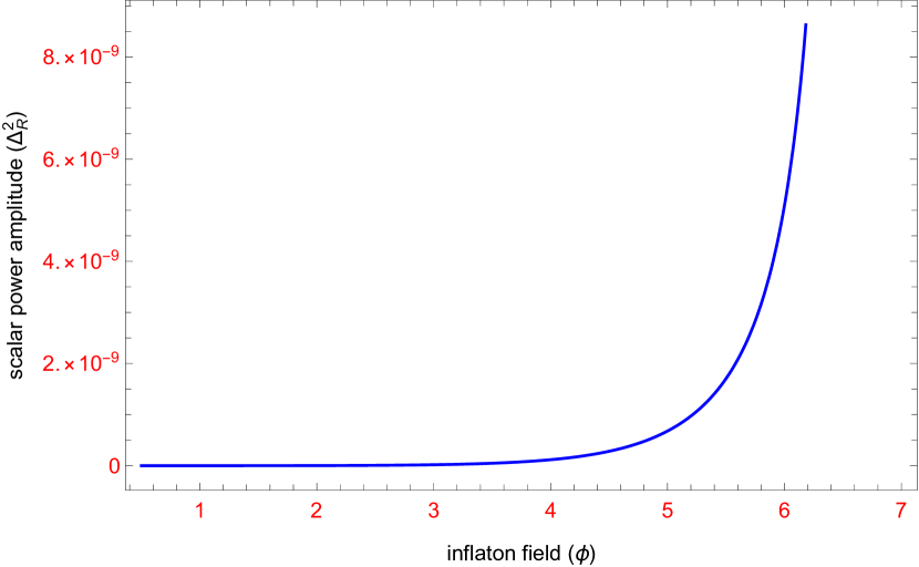
Figure 1: Plot of variation of scalar power amplitude ($\Delta_{R}^{2}$) with inflaton field ($\phi$)

.

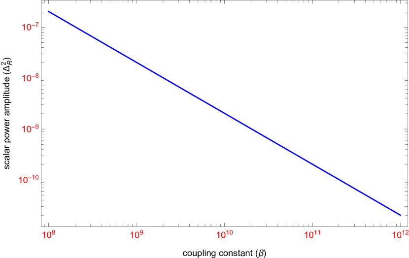
Figure 2: Plot of variation of scalar power amplitude($\Delta_{R}^{2}$) with coupling constant $\beta$

.

A careful observation reveals that the amplitude of the primordial scalar power spectrum which is related to the COBE normalization, $\Delta^{2}_{R}=2.1\times 10^{-9}$ [21] corresponds to the parameter space of the theory with the constraints $\beta\simeq 10^{10}$ $\frac{\gamma}{\beta^{2}}\simeq 10^{-5}$, and $\frac{\delta}{\beta^{3}}\simeq 10^{-7}$ at $\phi_{N}\simeq 5.5\,M_{Pl}$. We have mentioned that $\beta\equiv\frac{1}{{3{M^{2}}}}={10^{10}}$ corresponds to the energy scale or the mass scale of the inflationary model. The value of $\beta$ translates the mass scale of the theory to $M=5.8\times{10^{-6}}{M_{Pl}}\simeq 1.4\times{10^{13}}\,GeV$. We will use these particular values of the parameters throughout this paper. This is to be noted here that variation of $\beta$ from ${10^{8}}$ to ${10^{12}}$ correspond to the variation of mass-scale $M$ from $5.7\times{10^{-5}}\,M_{Pl}$ to $5.7\times{10^{-7}}\,M_{Pl}$.

The inflationary phase ends when either one or both the slow-roll conditions get violated. So $\epsilon=1$ and/ or $|\eta|=1$ can be safely considered as the end of inflation. Let us consider that the field at the end of inflation is $\phi_{end}$. Using the equations (11,12,22) we compute $\epsilon(\phi)$ and $|\eta(\phi)|$ varying $\phi$ and this variation is graphically shown in the plots of Fig.3. From the plot it is found that inflation ends at ${\phi_{end}}\simeq 0.75\,{M_{Pl}}$.

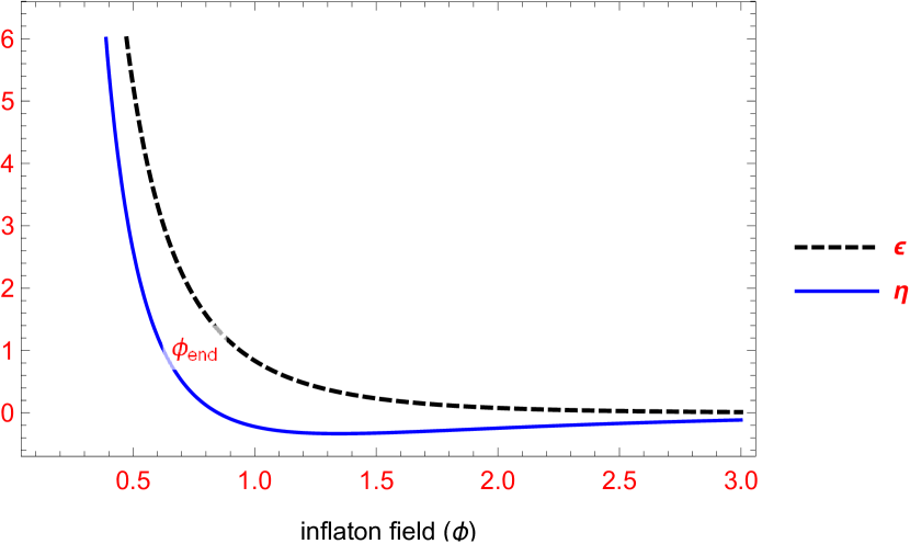
Figure 3: Plots of $\epsilon$ (black-dashed) and $\eta$ (blueline) with inflaton field ($\phi$)

The information of termination point ${\phi_{end}}\simeq 0.75\,{M_{Pl}}$ enables us to calculate the number of e-folds using the equations (14,22) with the information of the starting point of inflation $\phi_{N}=5.5M_{Pl}$ which we have already in hand. The following integral

$$N=\int_{0.75}^{5.5}{\frac{V}{{V^{\prime}}}}{\mkern 1.0mu}d\phi\simeq 63,$$ (24)

therefore, shows that the observable inflationary phase lasts for about 63 e-folds. We will examine in the next section whether this number is sufficient to solve the horizon problem.

Now we are in a position to present a pictorial demonstration of the inflationary model that emerges out from the calculations we have carried out so far. It is shown in Fig.4.

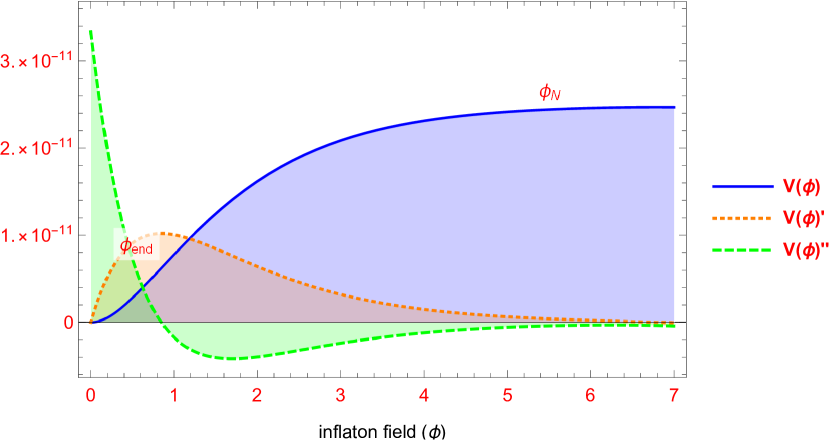
Figure 4: Plots of inflaton potential: $V(\phi)$ (Blue-solid), slope: $V(\phi)^{\prime}$ (Orange-dotted) and curvature: $V(\phi)^{\prime\prime}$ (Green-dotted) with inflaton field $\phi$

.

It shows that the observable inflation, i.e. the phase of inflation of our interest, starts with $\phi_{N}=5.5M_{Pl}$ and ends at around ${\phi_{end}}\simeq 0.75\,{M_{Pl}}$. It is worth mentioning that inflation initiates with a super-Planckian stage of the inflaton field $\phi$ and ends at the sub-Plackian stage. Total excursion of the field during inflation is $\Delta\phi\simeq 6.25\,{M_{Pl}}$ and during this phase the universe expands about 63 e-fold.

We have given a plot of variation of the inflaton potential $V(\phi)$ with $\phi$. The variation of the slope of the potential $V(\phi)^{\prime}$ and the curvature of the potential $V(\phi)^{\prime\prime}$ with $\phi$ is also shown in the same plot. These three curves in Fig.4, plays an important role to estimate the value of the slow-roll parameters in one hand and helps to have an idea of how the experimental observable behave on the other. This nature of the inflaton potential mimics that of Starbonsky-Whitt potential [38]. The potential looks reasonably flat for the successful slow-rolling of the inflaton field. It is also to be noted that the slope of the curve is positive. If it is not so then the integral formula of Eq.14 fails. Inflationary models with such ”Plateau type” potentials with concave curvature, $V^{\prime\prime}<0$, are most preferred by cosmological observations [21, 23, *chowdhury2019assessing] than the other types.

Now, we calculate the values of scalar tilt $n_{s}$ and tensor to scalar ratio $r$ that our model yields. The values are respectively given by:

$${n_{s}}\equiv{\left.{1-6\epsilon\left({{\phi_{N}}}\right)+2\eta\left({{\phi_{N}}}\right)}\right|_{{\phi_{N}}=5.5}}={\rm{0}}.{\rm{966242}}$$

and

$${\left.{r\equiv 16\epsilon\left({{\phi_{N}}}\right)}\right|_{{\phi_{N}}=5.5}}=0.00242$$

In Fig.5 we exhibit the variation of $n_{s}$ and $r$ with respect to $\phi$ and $\beta$ respectively.

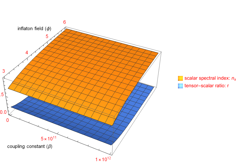
Figure 5: Plot of spectral index: $n_{s}$ (upper surface) and tensor to scalar ratio: $r$ (lower surface) with coupling constant $\beta$ and inflaton field $\phi$

.

From the figure, we can have an idea of how the spectral index and tensor-scalar ratio depends on $\phi$. The plots also exhibit the fact that the $n_{s}$ and $r$ are almost independent of the mass scale of the theory although the mass scale is fixed at $M=5.8\times 10^{-6}M_{Pl}$ which is needed to obtain the primordial scalar power spectrum that agrees with the experiment. We observe that the value $r$ and $n_{s}$ are $0.00242$ and $0.966242$ respectively at $\phi_{N}=5.5\,M_{Pl}$. These values are at par with the recent CMB observation [21], which tells that ${n_{s}}=0.9649\pm 0.0042$ and $r<0.06$. The predicted value of $r$ is also within Lyth bound [39] which demands, approximately,

$$r<0.003{\left({\frac{{50}}{N}}\right)^{2}}{\left({\Delta\phi}\right)^{2}}.$$

Putting $N=63$ and $\Delta\phi=6.25$ we get the bound: $r<0.073$. The value of $r$ predicted from our model is well within the Lyth bound.

If we compare our results from the predictions inferred from classic formulae of Starobinsky model [40, *Starobinsky:1983zz], it gives

$${n_{s}}\equiv 1-\frac{2}{N}=0.003023$$

and

$$r\equiv\frac{{12}}{{{N^{2}}}}=0.968253$$

for $N$=63. The small but noticeable difference in this result from the results we reported above is due to the inclusion of $R^{3}$ and $R^{4}$ terms.

V Mass of the inflaton field, maximum reheating temperature and minimum number of e-folds

It would be instructive to get an estimation of the mass of the scalar field. For a viable theory, the mass of this scalar would be concomitant with the energy scale of the theory. Let us see how the mass of the scalar field can be estimated in this situation.

V.1 An estimation of the mass of the inflaton

It is reasonable to think without violating any physical principle that the mass term of the inflaton field $\phi$ is present implicitly within the potential 22. If a potential has the following expansion

$$V(\phi)={c_{1}}+{c_{2}}{\phi^{2}}+{c_{3}}{\phi^{2}}+{c_{4}}{\phi_{4}}+\cdot\cdot\cdot,$$ (25)

the coefficient of the squared power of the $\phi$ gives the mass for the real scalar field $\phi$ which reads

$$m_{\phi}=\sqrt{2c_{3}}.$$ (26)

at the classical level. Expanding the potential 22 in a series of $\phi$ around $\phi=0$, we find that the mass of the field comes out to ${m_{\phi}}=5.8\times{10^{-6}}{M_{Pl}}\simeq 1.4\times{10^{13}}\,GeV$ which is in agreement with the energy scale of the theory. This value of ${m_{\phi}}$ can be considered as a signature for our model. What happens when the inflation process terminates is known that the universe enters into the reheating phase. Let us have a glimpse of that with the estimation of maximum reheating temperature.

V.2 Estimation of maximum reheating temperature

When inflation comes to an end, the potential energy that causes the crucial slow-rolling starts to dissipate, setting the inflation field to oscillate quasi harmonically back and forth at the bottom region of the potential. As a result reheating [42, *motohashi2012reheating] of the universe gets started and that gives rise to the condition which becomes amenable to standard big bang cosmology with the creation of new particle . This state is known as the reheating phase. In this article, we will not study the reheating phase in finer detail but we will give an estimation of maximum reheating temperature of the Universe as suggested from this model.

The inflaton scalar decays to all Standard Model(SM) particles. As the ${m_{\phi}}\gg{m_{H}}$, where ${m_{H}}$ is the Higgs mass, the dominant contribution of this decay comes from the SM electroweak sector [44, 33]. The decay rate is given by [44, *cheong2020beyond]

$${\Gamma_{\phi}}\simeq\frac{{m_{\phi}^{3}}}{{48\pi}}$$ (27)

The reheating temperature, ${T_{re}}$ is related to this decay rate by the following relation [33]:

$${T_{re}}\simeq{\left({\frac{{90}}{{{\pi^{2}}{g_{*}}}}}\right)^{1/4}}\sqrt{{\Gamma_{\phi}}}$$ (28)

Here $g_{*}$ is the number of relativistic degrees of freedom of the particles created at that time due to rapid oscillation after the termination of slow-rolling. Assuming all the SM particles relativistic at this energy scale, we take $g_{*}=106.5$. Substituting the value of ${m_{\phi}}$ in in 27 and using 27, 28 we obtain the value ${T_{re}}=6.1\times{10^{-10}}{m_{Pl}}\simeq 1.5\times{10^{9}}\,GeV$.

V.3 Estimation of minimum number of e-folds

Having derived the value of maximum reheating temperature, ${T_{re}}$, we now evaluate the minimum number of e-folds required to solve the horizon problem. The quantity is denoted by ${N_{*}}$ which is the number of e-folds from horizon exit to the end of inflation. A model independent calculation of ${N_{*}}$, in a matter dominated universe, leads to the expression [45, 33, 36]:

$${N_{*}}=61.4-\frac{1}{{12}}\ln\left({\frac{{45{V_{*}}}}{{{\pi^{2}}{g_{*}}T_{re}^{4}}}}\right)-\ln\left({\frac{{V_{*}^{1/4}}}{{{H_{*}}}}}\right).$$ (29)

Here, ${H_{*}}$ is the Hubble rate that can be obtained from the relation

$${H_{*}}={\left({\frac{{{V_{*}}}}{3}}\right)^{1/3}}.$$

In the above relation, ${V_{*}}\equiv{V_{end}}\equiv V({\phi_{end}})=5.24\times{10^{-12}}$. Substituting all the values in 29 we finally obtain numerically the value of ${N_{*}}=49.7\simeq 50$. We obtained from an exact calculation, earlier in sec.IV, that the number of e-folds in this model gives $N=63$. So, It can be said that the value of $N$ obtained from this model is large enough to fit the requirement.

VI Brief comparison among $R+R^{2}$, $R+R^{2}+R^{3}$ and $R+R^{2}+R^{3}+R^{4}$ models

In this section, we discuss some of the salient features of thee $R+R^{2}$ and $R+R^{2}+R^{3}$ models and also provide a comparison of these two with the $R+R^{2}+R^{3}+R^{4}$ model in the same framework. For brevity, we use the notations $R2$, $R3$, and $R4$ to denote $R+R^{2}$, $R+R^{2}+R^{3}$, and $R+R^{2}+R^{3}+R^{4}$ model respectively. The rest of the discussion in this section follows from the theoretical inputs described in Sec.III-V.

In the original Starobinsky model $f(R)$ was taken as

$$f_{R2}(R)=R+\frac{R^{2}}{6M^{2}}=R+\frac{\beta}{2}R^{2}.$$ (30)

With a $R^{3}$ correction to the above model one gets

$$f_{R3}(R)=R+\frac{R^{2}}{6M^{2}}+\frac{\lambda_{3}}{6}\frac{R^{3}}{(3M^{2})^{3}}=R+\frac{\beta}{2}R^{2}+\frac{\gamma}{3}R^{3}.$$ (31)

The real solutions $\chi(\Phi)$ (20) corresponding to the models (30) and (31) are

$$\chi_{R2}(\Phi)=\frac{1-\Phi}{\beta},$$ (32)

$${\chi_{R3}}(\Phi)=\frac{{\sqrt{{\beta^{2}}+4\gamma\,\Phi-4\gamma}-\beta}}{{2\gamma}}$$ (33)

respectively. We derive the inflaton potential for $R2$ model that reads

$${V_{R3}}(\phi){\text{ = }}\frac{{{e^{-2\sqrt{\frac{2}{3}}\phi}}{{\left({{e^{\sqrt{\frac{2}{3}}\phi}}-1}\right)}^{2}}}}{{4\beta}}.$$ (34)

Similarly, we have the inflaton potential for$R3$ model:

$${V_{R3}}(\phi)=\frac{{{e^{-2\sqrt{\frac{2}{3}}\phi}}{{\left({\beta-\sqrt{{\beta^{2}}+4\gamma\left({{e^{\sqrt{\frac{2}{3}}\phi}}-1}\right)}}\right)}^{2}}\left({2\sqrt{{\beta^{2}}+4\gamma\left({{e^{\sqrt{\frac{2}{3}}\phi}}-1}\right)}+\beta}\right)}}{{48{\gamma^{2}}}}.$$ (35)

The known COBE normalization fixes the values of the coupling constants as $\beta\simeq{10^{10}}$ and $\gamma\simeq\frac{{{\beta^{2}}}}{{{{10}^{5}}}}$.

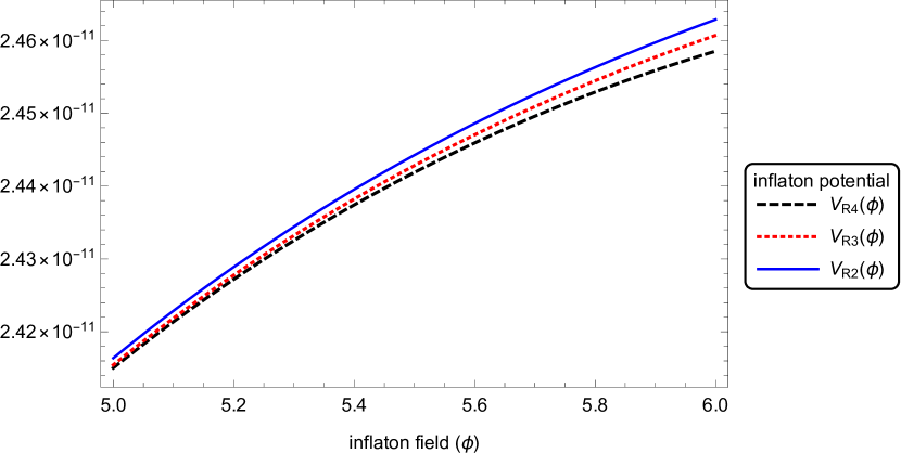
Figure 6: Plots of inflaton potential $V(\phi)$, for the models: $R4$ (Black-dashed), $R3$ (Red-dotted) and $R2$ (Blue-solid) with inflaton field $\phi$.

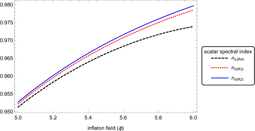
Figure 7: Plots of scalar spectral index $n_{s}$, for the models: $R4$ (Black-dashed), $R3$ (Red-dotted) and $R2$ (Blue-solid) with inflaton field $\phi$

.

Now, we are in a position to compare the potentials obtained in Eqs.(34,35,22). The plots are shown in Fig.6. We observe from the plots that the potentials corresponding to the models nearly overlap with each other at a lower value of $\phi$ but differ appreciably at higher values of the inflation field. This feature is expected since the inclusion of the higher order terms in $R$ in the model, automatically allows the entry of higher-order terms of the inflation field $\phi$. These extra higher order exponential terms play their crucial role in the potential in the vicinity of the starting of the inflation, which is $\phi_{N}=5.5M_{Pl}$ for this model. This small change in potential and the consequent changes in its slope, and curvature associated with it give rise to an adequate variation in the ’significant digit’ of the statistical data we are interested in. It is natural that these variations inevitably would have some influence in the process and that would certainly affect all the observables of interest, which have been established from our computation too. For an illustration, we are reporting only the calculations of scalar spectral index $n_{s}$ for $R2$, $R3$ and $R4$ models. We calculate the value of $n_{s}$ using Eqs.(15,11,12,34,35) and for the sake of comparison, we plot the values of $n_{s}$ for the three models. The plots are shown in Fig.7. In particular, if we calculate the value of $n_{s}$ at $\phi_{N}$ these come out as

$$\begin{array}[]{ccc}{n_{s(R2)}}=0.9690=0.9649+0.0041,\\ {n_{s(R3)}}=0.9683=0.9649+0.0034,\\ {n_{s(R4)}}=0.9662=0.9649+0.0013.\end{array}$$

It is evident from the above data that although the results calculated for the models involving $R2$, $R3$, and $R4$ are consistent with the experimentally observed value of $n_{s}$(PLANCK)=$0.9649\pm 0.0042$, the addition of $R^{3}$, and $R^{4}$ terms in the model provide a better fit to the result. These variations in data can be found in all the inflationary model parameters; furthermore, improvements are also expected in presence of additional higher terms in the model. It is true that the addition of a higher-order term helps to give a better fit because of the added free parameter involved in it. But this process can not be extended at our will, because the number of free parameters will go on increasing along with the increasing difficulties of solving the higher-order equations. So one has to be extremely judicious during handling the higher-order the term, however, according to the desired accuracy it can be apprehended up to which order term is needed to include. But these considerations are beyond the scope of the present work reported in this paper. Some of the references of such calculations are given in the introduction of this article.

VII Summary and Discussions

In this work, we have attempted to construct an inflationary mode that contains both $R^{3}$ and $R^{4}$ terms. Both the terms are treated as perturbation over $R^{2}$ term which was introduced by Starobinsky in his seminal work. We have computed the exact expression of potential, and the slow-rolling parameters without any approximation. Note that in the article [33, 30], the calculations were carried out with the leading order term of the potential. Our endeavor in our work leads us to a successful realization that Starobinsky type slow-roll inflation is feasible even in the simultaneous presence of both the $R^{3}$ and $R^{4}$ terms when the exact form of the potential is used for computation. In order to achieve slow-roll along with a good agreement with the experimentally observed value $\Delta_{R}^{2}=2.1\times{10^{-9}}$ the coefficient $\beta$, $\gamma$ and $\delta$ hade been found to be constrained. With the constants $\beta=10^{10}$ $\frac{\gamma}{\beta^{2}}=10^{-5}$, $\frac{\delta}{\beta^{3}}=10^{-7}$ we find that $r$ and $n_{s}$ comes out as $0.00242$ and $0.966242$ respectively when $\phi_{N}=5.5M_{Pl}$ is set. These values are in agreement with recent Planck data. However, the simultaneous presence of both $R^{3}$ and $R^{4}$ makes the number of e-fold a little higher, $N=63$, than that was predicted in the original Starobinsky model, but it is very close to the admissible range of the value of the e-fold number. A systematic evaluation of reheating temperature, which involves the calculation of the the decay rate of inflation to the Standard Model particles has also been carried out to predict the minimum number of e-folds r equired[18, 36, *martin2010first] in our model to solve the horizon problem. Our investigation establishes firmly that the inflation potential of this model does not destroy the classic characteristics of the Starobinsky model even after the inclusion of the term $R^{3}$ and $R^{4}$ in the original $R^{2}$-gravity model. All the interesting features of the Starobinsky model is found to occur significantly in the presence of both the $R^{3}$ and $R^{4}$. The reason for this behavior lies in the fact that making the the amplitude of scalar power, $\Delta_{R}^{2}$, ’COBE normalized’ suppresses the coefficients of $R^{3}$ and $R^{4}$ in comparison to $R^{2}$ term. We also observe that the effect of the presence of $R^{4}$ is small indeed like the contribution of $R^{3}$ but its effect would be treated in the same footing with the contribution of $R^{3}$.

We would like to reemphasize the summary of this work with some comments that are in order. $f(R)$ gravity theory with $R+R^{2}+R^{3}+R^{4}$ terms act as a consistent model of cosmological inflation. Reasonably satisfying agreement with experimental observations with the predictions of this model make it a phenomenologically viable one.