Exponential unitary integrators for nonseparable quantum Hamiltonians

Abstract

Quantum Hamiltonians containing nonseparable products of non-commuting operators, such as $\hat{\mbox{\boldmath${x}$}}^{m}\hat{\mbox{\boldmath${p}$}}^{n}$, are problematic for numerical studies using split-operator techniques since such products cannot be represented as a sum of separable terms, such as $T(\hat{\mbox{\boldmath${p}$}})+V(\hat{\mbox{\boldmath${x}$}})$. In the case of classical physics, Chin [Phys. Rev. E 80, 037701 (2009)] developed a procedure to approximately represent nonseparable terms in terms of separable ones. We extend Chin’s idea to quantum systems. We demonstrate our findings by numerically evolving the Wigner distribution of a Kerr-type oscillator whose Hamiltonian contains the nonseparable term $\hat{\mbox{\boldmath${x}$}}^{2}\hat{\mbox{\boldmath${p}$}}^{2}+\hat{\mbox{\boldmath${p}$}}^{2}\hat{\mbox{\boldmath${x}$}}^{2}$. The general applicability of Chin’s approach to any Hamiltonian of polynomial form is proven.

I Introduction

Split-operator methods Feit et al. (1982) are popular across many domains of physics because they combine the best of two worlds – simplicity of implementation and preservation of physical properties such as norm and energy. For the time evolution of Hamiltonian quantum systems (including those with nonlinearities Javanainen and Ruostekoski (2006)), unitary split-operator integrators Yoshida (1990) have emerged as reliable workhorses. However, such split-operator methods are currently restricted to Hamiltonians which are separable Cabrera et al. (2015), i.e. those that are a sum of two terms $T(\hat{\mbox{\boldmath${p}$}})$ and $V(\hat{\mbox{\boldmath${x}$}})$, each depending only on $\hat{\mbox{\boldmath${p}$}}$ and $\hat{\mbox{\boldmath${x}$}}$ respectively (throughout, we denote all quantum operators in bold face).

Other recent approaches treating nonseparable classical Hamiltonians exist, including one that yields good long time behaviour for classical dynamics, but which does this at the resource-intensive price of doubling up the phase space, see Tao (2016) and references therein. In the case of quantum systems this is too high a price to pay.

Classical evolution is governed by Poisson-brackets, whose commutators Chin’s method Chin (2009) combines algebraically such that upon application of exponential split-operator integrators it extends to the treatment of nonseparable Hamiltonians. Whilst such classical evolution is phase space volume-conserving Chin (2020) quantum evolution is not Oliva et al. (2017), and its evolution is governed by Moyal brackets. Therefore it remained unclear whether Chin’s approach can be adapted to quantum systems.

Here we show that Chin’s approach can be extended to quantum systems, see Sect. II, such as Kerr-oscillators, see Sect. III. In Sect. VI, we generalize its application to (nonseparable) Hamiltonians composed of polynomials. We use Wigner’s quantum phase space representation Curtright et al. (2014) and investigate its numerical performance in Secs. IV and V and then conclude in Sect. VII.

II Extending Chin’s approach to quantum evolution

II.1 From separable to nonseparable propagators

Separable Hamiltonians of the form $\hat{\mbox{\boldmath${H}$}}=T(\hat{\mbox{\boldmath${p}$}})+V(\hat{\mbox{\boldmath${x}$}})$ allow for operator splitting. Here, we deal with classical and quantum operators as well as their eigenvalues. Following Cabrera et al. (2015), we therefore adopt the following notation. Throughout, bold lettering ($\bm{x},\bm{p}$) refers to quantum scalars whereas regular lettering ($x,p$) refers to their classical counterparts or functions, such as $T$ or $V.$ Hats [($\hat{\mbox{\boldmath${p}$}}$, $\hat{\mbox{\boldmath${x}$}}$) vs. ($\hat{p}$, $\hat{x}$)] indicate their respective operators.

A state is propagated through a small time-step, $\varepsilon=-i\Delta t/\hbar$, by the unitary propagator $\hat{\mbox{\boldmath${U}$}}(\varepsilon)$. $\hat{\mbox{\boldmath${U}$}}$ can be split into the approximate form Chin (2009); Yoshida (1990)

$$\hat{\mbox{\boldmath${U}$}}(\varepsilon)={\rm e}^{\varepsilon\hat{\mbox{\boldmath${H}$}}}={\rm e}^{\varepsilon(\hat{\mbox{\boldmath${T}$}}+\hat{\mbox{\boldmath${V}$}})}\approx\prod_{i=1}^{N}{\rm e}^{t_{i}\varepsilon\hat{\mbox{\boldmath${T}$}}}{\rm e}^{v_{i}\varepsilon\hat{\mbox{\boldmath${V}$}}}={\rm e}^{\varepsilon\hat{\mbox{\boldmath${H}$}}_{A}},$$ (1)

here $\hat{\mbox{\boldmath${T}$}}=T(\hat{\mbox{\boldmath${p}$}})$ and $\hat{\mbox{\boldmath${V}$}}=V(\hat{\mbox{\boldmath${x}$}})$. $\hat{\mbox{\boldmath${H}$}}_{A}$ approximates $\hat{\mbox{\boldmath${H}$}}$; since $\hat{\mbox{\boldmath${H}$}}_{A}$ must be hermitian, it has to have an even-power expansion in $\varepsilon$. Here, all operator-products are meant to be from left to right: $\prod_{i=1}^{N}\hat{\mbox{\boldmath${U}$}}_{i}=\hat{\mbox{\boldmath${U}$}}_{1}\hat{\mbox{\boldmath${U}$}}_{2}\cdots\hat{\mbox{\boldmath${U}$}}_{N}$.

Following Chin (2009), we will only consider symmetric factorisation schemes for (1) such that the weighting coefficients are either $t_{1}=0$ and $v_{i}=v_{N-i+1}$, $t_{i+1}=t_{N-i+1}$, or $v_{N}=0$ and $v_{i}=v_{N-i}$, $t_{i}=t_{N-i+1}$.

Then, according to the Baker-Campbell-Hausdorff formula Yoshida (1990), $\hat{\mbox{\boldmath${H}$}}_{A}$ has the form

$$\hat{\mbox{\boldmath${H}$}}_{A}=e_{{}_{T}}\hat{\mbox{\boldmath${T}$}}+e_{{}_{V}}\hat{\mbox{\boldmath${V}$}}+\varepsilon^{2}e_{{}_{TTV}}[\hat{\mbox{\boldmath${T}$}}\hat{\mbox{\boldmath${T}$}}\hat{\mbox{\boldmath${V}$}}]$$

$$\qquad\quad+\varepsilon^{2}e_{{}_{VTV}}[\hat{\mbox{\boldmath${V}$}}\hat{\mbox{\boldmath${T}$}}\hat{\mbox{\boldmath${V}$}}]+O(\varepsilon^{4})\;,$$ (2)

where condensed commutator brackets $[\hat{\mbox{\boldmath${T}$}}\hat{\mbox{\boldmath${T}$}}\hat{\mbox{\boldmath${V}$}}]\equiv[\hat{\mbox{\boldmath${T}$}},[\hat{\mbox{\boldmath${T}$}},\hat{\mbox{\boldmath${V}$}}]]$, $[\hat{\mbox{\boldmath${T}$}}\hat{\mbox{\boldmath${V}$}}\hat{\mbox{\boldmath${T}$}}\hat{\mbox{\boldmath${V}$}}]\equiv[\hat{\mbox{\boldmath${T}$}},[\hat{\mbox{\boldmath${V}$}},[\hat{\mbox{\boldmath${T}$}},\hat{\mbox{\boldmath${V}$}}]]]$, etc., are used. The coefficients $e_{{}_{T}}$, $e_{{}_{VTV}}$, etc., are functions of $\{t_{i}\}$ and $\{v_{j}\}$.

By choosing $\{t_{i}\}$ and $\{v_{j}\}$ such that $\sum_{i}t_{i}=0=\sum_{j}v_{j}$, we impose that

$$e_{{}_{T}}=e_{{}_{V}}=0.$$ (3)

If we also impose that $e_{{}_{VTV}}=0$, or $e_{{}_{TTV}}=0$, then the approximate propagator (1) codes for nonseparable Hamiltonians $\hat{\mbox{\boldmath${H}$}}_{A}$, either of the form

$$\hat{\mbox{\boldmath${H}$}}_{A}\approx\hat{\mbox{\boldmath${H}$}}_{TTV}\propto[\hat{\mbox{\boldmath${T}$}}\hat{\mbox{\boldmath${T}$}}\hat{\mbox{\boldmath${V}$}}]{\rm,\;\;or}\;\;\hat{\mbox{\boldmath${H}$}}_{A}\approx\hat{\mbox{\boldmath${H}$}}_{VTV}\propto[\hat{\mbox{\boldmath${V}$}}\hat{\mbox{\boldmath${T}$}}\hat{\mbox{\boldmath${V}$}}].$$ (4)

To summarise, combined separable terms in Eq. (1) can emulate specific nonseparable operator products (4).

Chin showed in Chin (2009) that the specific symmetric product of nine exponentials (1), with coefficients $v_{0}=-2(v_{1}+v_{2})$, $t_{1}=-t_{2}$, $v_{2}=-\frac{1}{2}v_{1}$ and $v_{1}=\frac{1}{t_{2}^{2}}$, enables us to remove the third order term $[\hat{\mbox{\boldmath${V}$}}\hat{\mbox{\boldmath${T}$}}\hat{\mbox{\boldmath${V}$}}]$, constituting a ‘two step forward one step back’ scenario. It leads to scaling $\Delta E\sim{\cal O}(\Delta t^{2/3})$ Chin (2009) (see Sect. V.1) and results in

$$\hat{\mbox{\boldmath${U}$}}_{9}(\varepsilon) \approx e^{\varepsilon v_{2}\hat{\mbox{\boldmath${V}$}}}e^{\varepsilon t_{2}\hat{\mbox{\boldmath${T}$}}}e^{\varepsilon v_{1}\hat{\mbox{\boldmath${V}$}}}e^{\varepsilon t_{1}\hat{\mbox{\boldmath${T}$}}}e^{\varepsilon v_{0}\hat{\mbox{\boldmath${V}$}}}e^{\varepsilon t_{1}\hat{\mbox{\boldmath${T}$}}}e^{\varepsilon v_{1}\hat{\mbox{\boldmath${V}$}}}e^{\varepsilon t_{2}\hat{\mbox{\boldmath${T}$}}}e^{\varepsilon v_{2}\hat{\mbox{\boldmath${V}$}}}$$ (5)

$$\approx \exp(\varepsilon^{3}[\hat{\mbox{\boldmath${T}$}}\hat{\mbox{\boldmath${T}$}}\hat{\mbox{\boldmath${V}$}}]+\varepsilon^{5}E_{5}+\varepsilon^{7}E_{7}+\dots)\ .$$

Here, $t_{2}$ is a free parameter that can be chosen to minimise errors introduced through $E_{5}$; following Chin (2009), we use $t_{2}=-6^{\frac{1}{3}}$.

II.2 Propagating a state in the Schrödinger picture

In split operator techniques, when a propagator $\exp[\varepsilon(T(\hat{\mbox{\boldmath${p}$}})+V(\hat{\mbox{\boldmath${x}$}}))]$, with a small time step $\varepsilon=-i\Delta t/\hbar$, is applied to state $\psi({\bm{x}},t)$, we end up applying the sequence of maps

$$\psi( {\bm{x}}, t+\Delta t)=\exp[\varepsilon(T(\hat{\mbox{\boldmath${p}$}})+V(\hat{\mbox{\boldmath${x}$}}))]\;\psi({\bm{x}},t)$$ (6)

$$\approx \exp(\varepsilon T(\hat{\mbox{\boldmath${p}$}}))\exp(\varepsilon V(\hat{\mbox{\boldmath${x}$}}))\;\psi({\bm{x}},t)$$

$$= \mathcal{F}_{{\bm{p}}\rightarrow{\bm{x}}}\exp(\varepsilon T({\hat{\mbox{\boldmath${p}$}}}))\;\mathcal{F}_{{\bm{x}}\rightarrow{\bm{p}}}\exp(\varepsilon V({\hat{\mbox{\boldmath${x}$}}}))\psi({\bm{x}},t).$$

Here, $\cal F$ denotes fast Fourier transforms (and their inverses, in obvious notation) central to the speedup and numerical stability associated with the use of split operator techniques. To give an example, expression (5) entails the application of $\cal F$ at eight times per step $\varepsilon$.

III Product terms in Kerr oscillator Hamiltonian

The single-mode Kerr oscillator, in its simplest form, has the energy of the harmonic oscillator squared and is therefore analytically fully solvable. Explicitly, its Hamiltonian has the form

$$\hat{\mbox{\boldmath${H}$}}_{\textrm{Kerr}}=\left(\frac{\hat{\mbox{\boldmath${p}$}}^{2}}{2}+\frac{\hat{\mbox{\boldmath${x}$}}^{2}}{2}\right)^{2}=\frac{\hat{\mbox{\boldmath${p}$}}^{4}}{4}+\frac{[\hat{\mbox{\boldmath${p}$}}^{2},\hat{\mbox{\boldmath${x}$}}^{2}]_{+}}{4}+\frac{\hat{\mbox{\boldmath${x}$}}^{4}}{4},$$ (7)

where we used the anti-commutator $[\hat{a},\hat{b}]_{+}\equiv\hat{a}\hat{b}+\hat{b}\hat{a}$. The quantum Kerr effect comes about due to the self-interaction of photons in nonlinear media Kirchmair et al. (2013). Its dynamics is non-trivial and periodic with a recurrence time of $\tau=\frac{\pi}{\hbar}$; its phase space current follows circles Oliva and Steuernagel (2019a).

We now show that its nonseparable terms $[\hat{\mbox{\boldmath${p}$}}^{2},\hat{\mbox{\boldmath${x}$}}^{2}]_{+}$ can be cast into the shape of $\hat{\mbox{\boldmath${H}$}}_{A}$ in Eq. (2). To first order in the time step $\varepsilon=-i\Delta t/\hbar$, the Moyal bracket Cabrera et al. (2015); Oliva et al. (2017) of quantum phase space dynamics agrees with the classical Poisson bracket Chin (2009); Oliva et al. (2017). We therefore have to hope that the commutator $[\hat{\mbox{\boldmath${T}$}}\hat{\mbox{\boldmath${T}$}}\hat{\mbox{\boldmath${V}$}}]$ in Eq. (5) behaves similarly to the classical Poisson bracket–based Lie operators analysed by Chin Chin (2009).

Following Ref. Chin (2009), we therefore try the ansatz of a second order polynomial for $\hat{\mbox{\boldmath${T}$}}$ and a fourth order polynomial for $\hat{\mbox{\boldmath${V}$}}$. The choices $\hat{\mbox{\boldmath${T}$}}=\frac{c_{T}}{2\sqrt{2}}\hat{\mbox{\boldmath${p}$}}^{2}$ and $\hat{\mbox{\boldmath${V}$}}=\frac{c_{V}}{12}\hat{\mbox{\boldmath${x}$}}^{4}$ yield $[\hat{\mbox{\boldmath${T}$}}\hat{\mbox{\boldmath${T}$}}\hat{\mbox{\boldmath${V}$}}]=\frac{c_{T}^{2}c_{V}}{96}(\hat{\mbox{\boldmath${x}$}}^{4}\hat{\mbox{\boldmath${p}$}}^{4}+\hat{\mbox{\boldmath${p}$}}^{4}\hat{\mbox{\boldmath${x}$}}^{4}-2\;\hat{\mbox{\boldmath${p}$}}^{2}\hat{\mbox{\boldmath${x}$}}^{4}\hat{\mbox{\boldmath${p}$}}^{2})$. With $c_{T}=1=c_{V}$ and using Heisenberg’s commutation relation $[\hat{\mbox{\boldmath${p}$}},\hat{\mbox{\boldmath${x}$}}]=\frac{\hbar}{\rm i}$ this simplifies (we used Mathematica Muñoz and Delgado (2016)) to

$$[\hat{\mbox{\boldmath${T}$}}\hat{\mbox{\boldmath${T}$}}\hat{\mbox{\boldmath${V}$}}]=-\frac{\hbar^{4}}{4}-\frac{\hbar^{2}}{4}[\hat{\mbox{\boldmath${p}$}}^{2},\hat{\mbox{\boldmath${x}$}}^{2}]_{+},$$ (8)

with a real-valued constant term which gives rise to a global phase that can be ignored or subtracted out.

Alternatively, one can, for example, use $\hat{\mbox{\boldmath${T}$}}=\frac{\hat{\mbox{\boldmath${p}$}}^{4}}{24}+\frac{\hat{\mbox{\boldmath${p}$}}^{2}}{2}\text{ and }\hat{\mbox{\boldmath${V}$}}=\frac{\hat{\mbox{\boldmath${x}$}}^{2}}{2\sqrt{2}}$ while swapping $\hat{\mbox{\boldmath${V}$}}\leftrightarrow\hat{\mbox{\boldmath${T}$}}$ in expression (5), the formal result is the same (8), but numerical performance can differ slightly Bon .

We have thus established that a propagator using the separable terms $\hat{\mbox{\boldmath${T}$}}$ and $\hat{\mbox{\boldmath${V}$}}$ in $\hat{\mbox{\boldmath${U}$}}$, in Eq. (1), can generate a propagator featuring the product term $[\hat{\mbox{\boldmath${p}$}}^{2},\hat{\mbox{\boldmath${x}$}}^{2}]_{+}$, which represents the nonseparable middle term of the Kerr Hamiltonian in Eq. (7).

IV Propagation of mixed states using Wigner’s phase space approach

Instead of limiting ourselves to pure states propagated in the Schrödinger picture, as in Sect. II.2, we now study the time evolution of general quantum states $W(x,p,t)$, in Wigner’s phase space representation.

We employ Wigner’s representation for the following four reasons: firstly, many dissipative systems use coupling terms of product form, so Chin’s approach allows us to avoid iterations such as those as used in Eqs. (63) and (64) of Cabrera et al. (2015). Secondly, the Wigner representation describes mixed systems which result from such dissipative couplings. Thirdly, it can be efficiently implemented (in Schrödinger equation-like form, see below and Cabrera et al. (2015)). Finally, comparison of the quantum with Chin’s classical description becomes transparent when using the Wigner representation since it describes $W$’s dynamics using Moyal brackets Moyal (1949), the quantum analogue of Poisson brackets:

$$\frac{\partial W}{\partial t}=\{\!\!\{{H},W\}\!\!\}=\frac{1}{\rm i\hbar}\hat{\cal G}[W]\;.$$ (9)

Here, the Hamiltonian $H$, is given by the Wigner transform Hancock et al. (2004) of $\hat{\mbox{\boldmath${H}$}}$, which in the case of the Kerr Hamiltonian (7) is ${H}=\left(\frac{{p}^{2}}{2}+\frac{{x}^{2}}{2}\right)^{2}-\frac{\hbar^{2}}{4}$. The generator of motion $\hat{\cal G}$ is the Lie superoperator associated with the Moyal bracket Curtright et al. (2014), namely

$$\{\!\!\{f,g\}\!\!\} \equiv\frac{f\star g-g\star f}{i\hbar}$$

$$=\frac{2}{\hbar}f(x,p)\sin\left[\frac{\hbar}{2}\left(\overleftarrow{\frac{\partial}{\partial x}}\overrightarrow{\frac{\partial}{\partial p}}-\overleftarrow{\frac{\partial}{\partial p}}\overrightarrow{\frac{\partial}{\partial x}}\right)\right]g(x,p),$$ (10)

where $\star$ denotes the Groenewold-Moyal product Groenewold (1946); Curtright et al. (2014)

$$\star \equiv\exp\left[\frac{i\hbar}{2}\left(\overleftarrow{\frac{\partial}{\partial x}}\overrightarrow{\frac{\partial}{\partial p}}-\overleftarrow{\frac{\partial}{\partial p}}\overrightarrow{\frac{\partial}{\partial x}}\right)\right]$$ (11)

$$=\sum_{n=0}^{\infty}\frac{(i\hbar)^{n}}{2^{n}n!}\left(\overleftarrow{\frac{\partial}{\partial x}}\overrightarrow{\frac{\partial}{\partial p}}-\overleftarrow{\frac{\partial}{\partial p}}\overrightarrow{\frac{\partial}{\partial x}}\right)^{n}$$ (12)

in which the arrows denote the ‘direction’ of differentiation: $f\overrightarrow{\frac{\partial}{\partial x}}g=g\overleftarrow{\frac{\partial}{\partial x}}f=f\frac{\partial}{\partial x}g$.

Taylor’s expansion of Moyal’s bracket (IV) yields

$$\{\!\!\{f,g\}\!\!\}=\{f,g\}+\mathcal{O}\left(\hbar^{n}[\mbox{derivatives}^{2n}]\Bigr{|}_{n\geq 2}\right).$$ (13)

To lowest order, this gives us Poisson’s bracket $\{f,g\}=\frac{\partial f}{\partial x}\frac{\partial g}{\partial p}-\frac{\partial f}{\partial p}\frac{\partial g}{\partial x}$ of classical mechanics. We see that in Wigner’s representation the time evolution is formally similar to that in the classical case treated by Chin Chin (2009). We mention in passing that sending $\hbar\downarrow 0$, for instance in Eq. (16), (also numerically) implements a classical propagator. Wigner’s representation is additionally of interest, because it can be treated efficiently numerically since Moyal’s equation of motion (9) can be cast into the form of a Schrödinger equation Cabrera et al. (2015); Kołaczek et al. (2020), see next Sect. V.

Equation (11) connects the Wigner transform Hancock et al. (2004); Curtright et al. (2014) of non-commutative Hilbert space operator products $f(\hat{\mbox{\boldmath${x}$}},\hat{\mbox{\boldmath${p}$}})\cdot g(\hat{\mbox{\boldmath${x}$}},\hat{\mbox{\boldmath${p}$}})$ with non-commutative $\star$-products $f(x,p)\star g(x,p)$ on phase space:

$$f(x,p)\star g(x,p) \Longleftrightarrow f(\hat{\mbox{\boldmath${x}$}},\hat{\mbox{\boldmath${p}$}})\cdot g(\hat{\mbox{\boldmath${x}$}},\hat{\mbox{\boldmath${p}$}}),$$ (14)

$$\{\!\!\{f(x,p),g(x,p)\}\!\!\} \Longleftrightarrow[f(\hat{\mbox{\boldmath${x}$}},\hat{\mbox{\boldmath${p}$}}),g(\hat{\mbox{\boldmath${x}$}},\hat{\mbox{\boldmath${p}$}})].$$ (15)

V Numerical considerations

In Wigner-Weyl transformed variables, we can give $\hat{\cal G}$ of Eq. (9) the explicit form Cabrera et al. (2015)

$$\hat{\cal G} = {H}\left(\hat{x}-\frac{\hbar}{2}\hat{\theta},\hat{p}+\frac{\hbar}{2}\hat{\lambda}\right)-{H}\left(\hat{x}+\frac{\hbar}{2}\hat{\theta},\hat{p}-\frac{\hbar}{2}\hat{\lambda}\right)\quad$$ (16)

$$\equiv \hat{H}_{-,+}-\hat{H}_{+,-}\quad,$$ (17)

with the commutation relations Cabrera et al. (2015); Bondar et al. (2012):

$${[}\hat{x},\hat{p}{]_{-}}=0,\quad{[}\hat{x},\hat{\lambda}{]_{-}}=i,\quad{[}\hat{p},\hat{\theta}{]_{-}}=i,\quad{[}\hat{\lambda},\hat{\theta}{]_{-}}=0\;,$$ (18)

which span a suitable Wigner-Weyl ‘Hilbert phase space’ Cabrera et al. (2015). Hence,

$$\hat{\cal U} = \exp\left(\varepsilon\left(\hat{H}_{-,+}-\hat{H}_{+,-}\right)\right)\;,$$ (19)

and for time-independent Hamiltonians

$$W(t)=\exp{\left(-i\frac{t-t_{0}}{\hbar}\hat{\cal G}\right)}[W(t_{0})]=\hat{\cal U}[W(t_{0})]\;.$$ (20)

We emphasise that in choosing the $(x,\theta)$-representation Cabrera et al. (2015), for Eq. (18), using suitable Bopp operators Bopp (1956)

$$\hat{x}=x,\quad\hat{p}=i\frac{\partial}{\partial\theta},\quad\hat{\lambda}=-i\frac{\partial}{\partial x},\text{ and }\;\hat{\theta}=\theta,\quad$$ (21)

Eq. (9) becomes Schrödinger equation-like, making it possible to apply efficient numerical propagation employing fast Fourier transform methods Cabrera et al. (2015); Arnold and Ringhofer (1996); Thomann and Borzì (2017); Kołaczek et al. (2020). This is very useful for systems that cannot be modelled as pure states, such as in the presence of decoherence.

Using $\hat{P}_{\pm}\equiv\hat{p}\pm\frac{\hbar}{2}\hat{\lambda}$ and $\hat{X}_{\pm}\equiv\hat{x}\pm\frac{\hbar}{2}\hat{\theta}$, we can express $\hat{\cal U}$ (19) for the Kerr Hamiltonian (7) as

$$\hat{\cal U}_{\textrm{Kerr}} = \exp{\left[\frac{\varepsilon}{4}\left(\hat{P}_{+}^{4}-\hat{P}_{-}^{4}+\left[\hat{P}_{+}^{2}\hat{X}_{-}^{2}-\hat{P}_{-}^{2}\hat{X}_{+}^{2}+\hat{X}_{-}^{2}\hat{P}_{+}^{2}-\hat{X}_{+}^{2}\hat{P}_{-}^{2}\right]+\hat{X}_{-}^{4}-\hat{X}_{+}^{4}\right)\right]}$$ (22a)

$$= \exp{\left[\frac{\varepsilon}{4}\left(\hat{P}_{+}^{4}-\hat{P}_{-}^{4}\right)\right]}\exp{\left[\frac{\varepsilon}{4}\left([\hat{P}_{+}^{2},\hat{X}_{-}^{2}]_{+}-[\hat{P}_{-}^{2},\hat{X}_{+}^{2}]_{+}\right)\right]}\exp{\left[\frac{\varepsilon}{4}\left(\hat{X}_{-}^{4}-\hat{X}_{+}^{4}\right)\right]}\;+{\cal O}(\varepsilon^{2})\;\;.$$ (22b)

According to Eq. (8), the appearance of anti-commutators in the middle exponential of expression (22b) allows us to express the contribution from the central product term in the Kerr Hamiltonian (7) as a single product of form (5); for an efficient implementation in Python see Bon .

V.1 Error Scaling for Kerr System

In the following, we set $\hbar=1$ and use coherent states

$$W\left(x,p,t=0\right)=\frac{1}{\pi}\exp\left(-(x-x_{0})^{2}-(p-p_{0})^{2}\right)$$ (23)

as initial states. For an example of their time evolution, see Fig. 1.

Using exponential propagators (whose action is time-reversible), we confirmed that Chin’s approach preserves the state’s norm at machine precision.

We checked for energy and phase stability, varying the time step $\Delta t$. In the case of a classical system with similar structure Chin reports Chin (2009), in accord with Eq. (5), scaling with order ${\cal O}(\varepsilon^{5})/{\cal O}(\varepsilon^{3})\sim{\cal O}(\Delta t^{2/3})$; this is roughly what we observed here, in the quantum Kerr case, as well.

The period of our Kerr system is $\pi$, see Fig. 1 (c). As a proxy for phase drift, associated with this algorithm, we determine the wave function overlap at recurrence times $\tau=\pi$ and find that $1-\langle W_{\rm exact}(0)|W(\tau)\rangle\sim{\cal O}(\Delta t^{1.2})$, a scaling better than that of the energy fluctuations (we distinguish between $W_{\rm exact}$ and the numerically propagated distribution $W$). For this we could not find a quantitative explanation. We also numerically propagated $\psi$ and confirmed that $1-|\langle\psi_{\rm exact}(0)|\psi(\pi)\rangle|^{2}\sim{\cal O}(\Delta t^{1.2})$ follows the same scaling as the Wigner function propagator. To make sure there is nothing special about one complete revolution we also checked for $\tau=\pi/2$, $1-\langle W_{\rm exact}(\pi/2)|W(\tau)\rangle\sim{\cal O}(\Delta t^{1.2})$, the behaviour is the same. Alternatively, $\langle W_{\rm exact}(0)-W(\tau)|W_{\rm exact}(0)-W(\tau)\rangle^{1/2}$ and max${}_{x,p}|W_{\rm exact}(x,p,0)-W(x,p,\tau)|$, used as overlap measures, yield error scaling $\sim{\cal O}(\Delta t^{2/3})$ and, again, behave the same whether running for one complete revolution or otherwise. For details see Ref. Bon .

V.2 Modification of Chin’s expression

In the Kerr-case studied here, it is possible to modify Chin’s expression (5) by removing first and last terms yielding the approximation

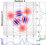
Figure 1: Kerr system (7) evolves an initial coherent state (23) with amplitude ‘3’ [$W_{0}(x_{0}=3/\sqrt{2},p_{0}=3/\sqrt{2})$] using timesteps $\Delta t=0.0001$ in columns (a) to (c) and $\Delta t=0.0015$ in column (d). We observe that the initial state recurs at the system’s recurrence time $\tau=\pi$ columns (c) and (d) and fractional revivals of the initial states with approximate three-fold symmetry Oliva and Steuernagel (2019b); Averbukh and Perelman (1989); Robinett (2004) form at times $\tau/3$ and $2\tau/4$, see columns (a) and (b), respectively. The same parameters are used in top and bottom row, except that the top row employs the more accurate propagator $\hat{\mbox{\boldmath${U}$}}_{9}$ of Eq. (5) whereas the bottom row uses $\hat{\mbox{\boldmath${U}$}}_{7}$ of Eq. (24a), the numerical errors become more pronounced with both, increasing propagation time and increasing timesteps.

$$\hat{\mbox{\boldmath${U}$}}_{7}(\varepsilon) = e^{\varepsilon t_{2}\hat{\mbox{\boldmath${T}$}}}e^{\varepsilon v_{1}\hat{\mbox{\boldmath${V}$}}}e^{\varepsilon t_{1}\hat{\mbox{\boldmath${T}$}}}e^{\varepsilon v_{0}\hat{\mbox{\boldmath${V}$}}}e^{\varepsilon t_{1}\hat{\mbox{\boldmath${T}$}}}e^{\varepsilon v_{1}\hat{\mbox{\boldmath${V}$}}}e^{\varepsilon t_{2}\hat{\mbox{\boldmath${T}$}}}\qquad$$ (24a)

$$= \hat{\mbox{\boldmath${U}$}}_{9}(\varepsilon)-\frac{\varepsilon^{3}}{t_{2}^{3}}[\hat{\mbox{\boldmath${V}$}}\hat{\mbox{\boldmath${V}$}}\hat{\mbox{\boldmath${T}$}}]+{\cal O}(\varepsilon^{5}).$$ (24b)

We use the modified coefficients $v_{0}=-2v_{1}$, $t_{1}=-t_{2}$, $v_{1}=\frac{1}{t_{2}^{2}}$, and again $\hat{\mbox{\boldmath${T}$}}=\frac{c_{T}}{2\sqrt{2}}\hat{\mbox{\boldmath${p}$}}^{2}$ and $\hat{\mbox{\boldmath${V}$}}=\frac{c_{V}}{12}\hat{\mbox{\boldmath${x}$}}^{4}$, with the final result Muñoz and Delgado (2016)

$$\hat{\mbox{\boldmath${U}$}}_{7}(\varepsilon) =1+\varepsilon^{3}\left(-\frac{\hbar^{4}}{4}-\frac{\hbar^{2}}{4}[\hat{\mbox{\boldmath${p}$}}^{2},\hat{\mbox{\boldmath${x}$}}^{2}]_{+}+\frac{\hbar^{2}}{9\sqrt{2}\,t_{2}^{3}}\hat{\mbox{\boldmath${x}$}}^{6}\right)+{\cal O}(\varepsilon^{5}).\qquad$$ (25)

This is similar to result (8). We have to compensate for the unwanted term in $\hat{\mbox{\boldmath${x}$}}^{6}$, by subtracting $\frac{\hbar^{2}}{9\sqrt{2}\,t_{2}^{3}}\hat{\mbox{\boldmath${x}$}}^{6}$ from potential terms in Eqs. (6) and (22b), but gain the advantage of having to numerically calculate fewer terms.

Whether a form like (24a) that is as useful as (25) can be found in the general case, we do not know at this stage. We emphasise that $\hat{\mbox{\boldmath${U}$}}_{7}$ has fewer product terms and runs a little faster but also performs worse than $\hat{\mbox{\boldmath${U}$}}_{9}$ of Eq. (5) in absolute terms, see Fig. 1. The errors in energy and phase both scale roughly with ${\cal O}(\Delta t^{2/3})$, similarly to and worse than in the case of $\hat{\mbox{\boldmath${U}$}}_{9}$, respectively.

For more details consult our code Bon , further discussions of such questions is beyond the scope of this work.

VI Chin’s approach is general

In order to show that Chin’s approach is generally applicable, let us prove

Theorem 1.

Any polynomial ${\Pi}(\hat{\mbox{\boldmath${x}$}},\hat{\mbox{\boldmath${p}$}})$ of $\hat{\mbox{\boldmath${x}$}}$ and $\hat{\mbox{\boldmath${p}$}}$ can be written as a finite linear combination of $[\hat{\mbox{\boldmath${x}$}}^{n}\hat{\mbox{\boldmath${x}$}}^{n}\hat{\mbox{\boldmath${p}$}}^{m}]\equiv[\hat{\mbox{\boldmath${x}$}}^{n},[\hat{\mbox{\boldmath${x}$}}^{n},\hat{\mbox{\boldmath${p}$}}^{m}]]$ and $[\hat{\mbox{\boldmath${p}$}}^{m}\hat{\mbox{\boldmath${x}$}}^{n}\hat{\mbox{\boldmath${p}$}}^{m}]\equiv[\hat{\mbox{\boldmath${p}$}}^{m},[\hat{\mbox{\boldmath${x}$}}^{n},\hat{\mbox{\boldmath${p}$}}^{m}]]$.

Proof.

Let us provide a constructive proof. A polynomial $\Pi(\hat{\mbox{\boldmath${x}$}},\hat{\mbox{\boldmath${p}$}})$ is Weyl-transformed Hancock et al. (2004) to $P(x,p)$ in phase space, according to Eq. (14). Assume $x^{N}p^{M}$ is its leading term, namely, $P(x,p)$ is a polynomial of order $(N,M)$.

Via Eq. (15), a double commutator $[\hat{\mbox{\boldmath${x}$}}^{n}\hat{\mbox{\boldmath${x}$}}^{n}\hat{\mbox{\boldmath${p}$}}^{m}]$ corresponds to $\{\!\!\{x^{n},\{\!\!\{x^{n},p^{m}\}\!\!\}\}\!\!\}$. In fact, the latter are polynomials because the Moyal bracket (IV) is obtained by differentiating its arguments. According to Eq. (13), the leading term of the polynomial $\{\!\!\{x^{n},p^{m}\}\!\!\}$ is $x^{n-1}p^{m-1}$; hence, the leading term of $\{\!\!\{x^{n},\{\!\!\{x^{n},p^{m}\}\!\!\}\}\!\!\}$ is $x^{2n-2}p^{m-2}$. Likewise, a double commutator $[\hat{\mbox{\boldmath${p}$}}^{m}\hat{\mbox{\boldmath${x}$}}^{n}\hat{\mbox{\boldmath${p}$}}^{m}]$ corresponds to the polynomial $\{\!\!\{p^{m},\{\!\!\{x^{n},p^{m}\}\!\!\}\}\!\!\}$ with the leading term of order $x^{n-2}p^{2m-2}$.

The set of polynomials

$$\Big{[}\{\!\!\{x^{n},\{\!\!\{x^{n},p^{m}\}\!\!\}\}\!\!\},\{\!\!\{p^{m},\{\!\!\{x^{n},p^{m}\}\!\!\}\}\!\!\}\Big{]}_{n=1,2,\ldots,N+2}^{m=1,2,\ldots,M+2}$$ (26)

is linearly independent and large enough to span the set of polynomials of order $(N,M)$, including $P(x,p)$. ∎

We observe that in the above proof all Moyal brackets $\{\!\!\{.,.\}\!\!\}$ can be substituted by Poisson brackets $\{.,.\}$ whilst leaving the argument intact: Chin’s approach applies to polynomial classical hamiltonians as well.

Theorem 1 prescribes how any polynomial quantum Hamiltonian can be decomposed into the Hamiltonians of the form (4). Hence, Chin’s algorithm is very general.

VII Conclusion

We have shown that Chin’s method Chin (2009) for the propagation of classical nonseparable Hamiltonians can be adopted to quantum systems. Chin’s method is general, and therefore allows for the universal treatment of nonseparable Hamiltonians using split-operator techniques. Chin’s method should be especially well suited for numerical simulations of large open quantum systems using stochastic Schrödinger equations Jacobs and Steck (2006) since their errors scale poorly.

Data Availability Statement

The codes developed for the current study are available at Bon .

References

- Feit et al. (1982) M. Feit, J. Fleck Jr, and A. Steiger, J. Comp. Phys. 47, 412 (1982).
- Javanainen and Ruostekoski (2006) J. Javanainen and J. Ruostekoski, J. Phys. A: Math. Gen. 39, L179 (2006).
- Yoshida (1990) H. Yoshida, Phys. Lett. A 150, 262 (1990).
- Cabrera et al. (2015) R. Cabrera, D. I. Bondar, K. Jacobs, and H. A. Rabitz, Phys. Rev. A 92, 042122 (2015), 1212.3406 .
- Tao (2016) M. Tao, Phys. Rev. E 94, 043303 (2016).
- Chin (2009) S. A. Chin, Phys. Rev. E 80, 037701 (2009).
- Chin (2020) S. A. Chin, Am. J. Phys. 88, 883 (2020).
- Oliva et al. (2017) M. Oliva, D. Kakofengitis, and O. Steuernagel, Physica A 502, 201 (2017), 1611.03303 .
- Curtright et al. (2014) T. L. Curtright, D. B. Fairlie, and C. Zachos, A Concise Treatise on Quantum Mechanics in Phase Space (World Scientific, 2014).
- Kirchmair et al. (2013) G. Kirchmair, B. Vlastakis, Z. Leghtas, S. E. Nigg, H. Paik, E. Ginossar, M. Mirrahimi, L. Frunzio, S. M. Girvin, and R. J. Schoelkopf, Nature 495, 205 (2013), 1211.2228 .
- Oliva and Steuernagel (2019a) M. Oliva and O. Steuernagel, Phys. Rev. A 99, 032104 (2019a), arXiv:1811.02952 [quant-ph] .
- Muñoz and Delgado (2016) J. G. Muñoz and F. Delgado, J. Phys. Conf. Ser. 698, 012019 (2016).
- (13) https://github.com/dibondar/NonseparableSplitOperator.
- Moyal (1949) J. E. Moyal, Proc. Cambridge Philos. Soc. 45, 99 (1949).
- Hancock et al. (2004) J. Hancock, M. A. Walton, and B. Wynder, Eur. J. Phys. 25, 525 (2004), physics/0405029 .
- Groenewold (1946) H. J. Groenewold, Physica 12, 405 (1946).
- Kołaczek et al. (2020) D. Kołaczek, B. J. Spisak, and M. Wołoszyn, in Information Technology, Systems Research, and Computational Physics, edited by P. Kulczycki, J. Kacprzyk, L. T. Kóczy, R. Mesiar, and R. Wisniewski (Springer International Publishing, Cham, 2020) pp. 307–320.
- Bondar et al. (2012) D. I. Bondar, R. Cabrera, R. R. Lompay, M. Y. Ivanov, and H. A. Rabitz, Phys. Rev. Lett. 109, 190403 (2012), 1105.4014v5 .
- Bopp (1956) F. Bopp, Annales de l’institut Henri Poincaré 15, 81 (1956).
- Arnold and Ringhofer (1996) A. Arnold and C. Ringhofer, SIAM J. Numer. Anal. 33, 1622 (1996).
- Thomann and Borzì (2017) A. Thomann and A. Borzì, Num. Meth. Part. Diff. Eq. 33, 62 (2017).
- Oliva and Steuernagel (2019b) M. Oliva and O. Steuernagel, Phys. Rev. Lett. 122, 020401 (2019b), 1708.00398 .
- Averbukh and Perelman (1989) I. S. Averbukh and N. F. Perelman, Phys. Lett. A 139, 449 (1989).
- Robinett (2004) R. W. Robinett, Phys. Rep. 392, 1 (2004).
- Jacobs and Steck (2006) K. Jacobs and D. A. Steck, Contemporary Phys. 47, 279 (2006).