SSM-Net: feature learning for Music Structure Analysis using a Self-Similarity-Matrix based loss

Abstract

In this paper, we propose a new paradigm to learn audio features for Music Structure Analysis (MSA). We train a deep encoder to learn features such that the Self-Similarity-Matrix (SSM) resulting from those approximates a ground-truth SSM. This is done by minimizing a loss between both SSMs. Since this loss is differentiable w.r.t. its input features we can train the encoder in a straightforward way. We successfully demonstrate the use of this training paradigm using the Area Under the Curve ROC (AUC) on the RWC-Pop dataset.

1 Introduction

Music Structure Analysis (MSA) is the task aiming at identifying musical segments that compose a music track (a.k.a. segment boundary estimation) and possibly label them based on their similarity (a.k.a. segment labeling). Over the years, systems for MSA have switched from

• hand-crafted detection system (checker-board-kernel [1] or DTW [2]) applied to hand-crafted audio features (MFCC or Chroma)

• to deep learning detection system (boundary detection using ConvNet [3, 4, 5]) applied to hand-crafted audio features, and recently

• to hand-crafted detection system (checker-board-kernel) applied to deep learned features [6, 7].

Among the paradigms used to learn these features, metric learning using the triplet loss [8] has been the most popular, either using unsupervised learning [6] or using supervised learning [7]. In this paper, we propose a new paradigm to learn these features, which is more straightforward and less-computationally expensive (on a GPU Tesla P100-PCIE, training in about 1 hour for our approach and 24 hours for [6]).

2 Proposal: SSM-Net

Our SSM-net system is illustrated in Figure 1. The inputs and architecture (but not the loss) of our system are inspired by McCallum’s work [6] (but largely simplified).

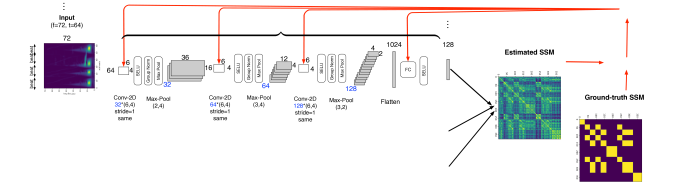
Figure 1: SSM-net architecture. From left to right: input sequence $\{\mathbf{X}_{i}\}$ of beat-synchronous CQT-patches, encoder $f^{\theta}$ applied to each $\mathbf{X}_{i}$, estimated SSM $\mathbf{\hat{S}}_{ij}^{\theta}$ computed with embeddings $\{\mathbf{e}^{\theta}_{i}\}=f^{\theta}(\{\mathbf{X}_{i}\})$, Loss $\mathcal{L}^{\theta}$ computation.

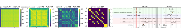
Figure 2: [Left] SSMs $\mathbf{\hat{S}}_{ij}^{\theta}$ computed using embeddings $\mathbf{e}^{\theta}$ obtained using (from left to right): cqt, mccallum-biased, ssmnet and ground-truth SSM $\mathbf{S}_{ij}$, on track 2 from RWC-Pop dataset. Loss $\mathcal{L}$ and AUC are indicated on top of each. [Right] Box-plots of Loss $\mathcal{L}$ and AUC obtained for all tracks of RWC-Pop dataset.

Input data $\{\mathbf{X}_{i}\}$. Each audio track is represented as a temporal sequence of $T$ audio features $\mathbf{X}_{i}$ which we denote as $\{\mathbf{X}_{i}\}_{i\in\{1\ldots T\}}$ or $\{\mathbf{X}_{i}\}$ for short. $\{\mathbf{X}_{i}\}$ are beat-synchronized patches of Constant-Q-Transform (CQT), each centered on a beat position $b_{i}$. Each patch represents 4 successive beats. Each beat is further sub-divided into 16 sub-beats. For this, the content of the CQTs between two successive beats $b_{i-1}$ and $b_{i}$ is analyzed and clustered into 16. The inputs to our network are therefore patches $\mathbf{X}_{i}$ of CQT, each of size (72 frequencies, 4*16 sub-beats) and centered on a beat $b_{i}$.

Network architecture $\mathbf{e}^{\theta}_{i}=f^{\theta}(\mathbf{X}_{i})$. The architecture of our encoder $f^{\theta}$ is illustrated in Figure 1. It comprises 3 consecutive blocks (L1, L2, L3) of a 2D convolution followed by a SELU [12] activation, a 2D group normalization [13] with 32 channels and a 2D max-pooling, The convolutional layers use a kernel size of (f=6, t=4) and the max-pooling layers use respectively kernel sizes of (2, 4), (3, 4) and (3, 2). The output is then passed to a single Fully-Connected (FC) layer of 128 units with a SELU activation. The output is then L2-normalized and constitutes the embedding $\mathbf{e}^{\theta}_{i}=f^{\theta}(\mathbf{X}_{i})$. $\theta$ denotes the set of parameters to be trained (348.400 parameters). For comparison the original McCallum [6] network has 1.280.768.

SSM-Net Loss. We apply the same encoder $f^{\theta}$ to each input $\mathbf{X}_{i}$. We then obtain the corresponding sequence of embeddings $\{\mathbf{e}^{\theta}_{i}\}_{i\in\{1\ldots T\}}=f^{\theta}(\{\mathbf{X}_{i}\}_{i\in\{1\ldots T\}})$. We can then easily construct an estimated SSM, $\mathbf{\hat{S}}_{ij}^{\theta}$, using a distance/similarity $g$ function between all pairs of projections:

$$\mathbf{\hat{S}}_{ij}^{\theta}=g(\mathbf{e}^{\theta}_{i}=f^{\theta}(\mathbf{X}_{i}),\mathbf{e}^{\theta}_{j}=f^{\theta}(\mathbf{X}_{j})),\;\;\;\forall i,j$$ (1)

$g$ is here a simple cosine-similarity which we scale to $[0,1]$:

$$\mathbf{\hat{S}}_{ij}^{\theta}=1-\frac{1}{4}\lVert\mathbf{e}^{\theta}_{i}-\mathbf{e}^{\theta}_{j}\rVert_{2}^{2}\;\;\;\in[0,1]$$ (2)

It is then possible to compare $\mathbf{\hat{S}}_{ij}^{\theta}$ to a ground-truth binary SSM, $\mathbf{S}_{ij}$. We formulate this as a multi-class problem (a set of $T^{2}$ binary classifications) and minimize the sum of Binary-Cross-Entropy (BCE) losses. We compensate the class unbalancing by using a weighting factor $\lambda$ computed as the percentage of 1 values in $\mathbf{S}_{ij}$.

$$\mathcal{L}^{\theta}\!=\!-\!\sum_{i,j=1}^{T}\!(1\!-\lambda)\!\left[\mathbf{S}_{ij}\!\log(\!\mathbf{\hat{S}}_{ij}^{\theta}\!)\!\right]\!+\!\lambda\!\left[\!(\!1\!-\!\mathbf{S}_{ij}\!)\!\log\!(\!1\!-\!\mathbf{\hat{S}}_{ij}^{\theta}\!)\!\right]$$ (3)

Since the computation of the SSM $\mathbf{\hat{S}}_{ij}^{\theta}$ is differentiable w.r.t. to the embeddings $\{\mathbf{e}^{\theta}_{i}\}$, we can compute $\frac{\partial\mathcal{L}^{\theta}}{\partial\theta}$

$$\frac{\partial\mathcal{L}^{\theta}}{\partial\theta}=\sum_{i,j=1}^{T}\frac{\partial\mathcal{L}^{\theta}}{\partial\mathbf{\hat{S}}_{ij}^{\theta}}\left(\frac{\partial\mathbf{\hat{S}}_{ij}^{\theta}}{\partial\mathbf{e}^{\theta}_{i}}\frac{\partial\mathbf{e}^{\theta}_{i}}{\partial\theta}+\frac{\partial\mathbf{\hat{S}}_{ij}^{\theta}}{\partial\mathbf{e}^{\theta}_{j}}\frac{\partial\mathbf{e}^{\theta}_{j}}{\partial\theta}\right)$$ (4)

Training. We minimize the loss using MADGRAD [14] with a learning rate of $5\!\times\!10^{-4}$, a weight decay of $10^{-2}$ and early-stopping. The mini-batch-size $m$ (here defined as the number of full-tracks) is set to 6.

Generating a ground-truth SSM $\mathbf{S}_{ij}$. To generate $\mathbf{S}_{ij}$, we rely on the homogeneity assumption, i.e. we suppose that all $t_{i}$ that fall within an annotated segment are identical since they share the same label. If we denote by $\text{seg}(t_{i})$ the segment $t_{i}$ belongs to and by $\text{label}(\text{seg}(t_{i}))$ its label, we assign the value $\mathbf{S}_{ij}=1$ if $\text{label}(\text{seg}(t_{i}))=\text{label}(\text{seg}(t_{j}))$.

3 Evaluation

To evaluate the quality of the features independently of the choice of a specific detection algorithm for MSA, we directly compare the ground-truth $\mathbf{S}_{ij}$ and the $\mathbf{\hat{S}}_{ij}^{\theta}$ obtained using various choices for $\mathbf{e}^{\theta}$. For each choice, we measure the obtained Loss $\mathcal{L}$ (lower is better) and AUC (higher is better) . We conside the following features $\mathbf{e}^{\theta}$:

• cqt: the flattened CQT patches $\{\mathbf{X}_{i}\}$

• convnet: the output of the un-trained (random weight) encoder $f^{\theta}$ applied to $\{\mathbf{X}_{i}\}$

• ssmnet: the output of $f^{\theta}$ trained with SSM-Net

• mccallum-normal/biased: the output of the same encoder $f^{\theta}$ but trained using the two unsupervised metric learning approaches described in [6]

• ssmnet-mccallum-normal/biased: same as for ssmnet but $f^{\theta}$ is pre-trained using mccallum-normal/biased

To train our SSM-Net, , we used a sub-set of 695 tracks from the labeled dataset Harmonix [15]. To train the unsupervised metric learning approach described in [6], we used a large unlabeled dataset from YouTube of 26.000 tracks from various genres.The evaluation is performed on RWC-Pop [16] labeled with AIST annotations [17]).

In Figure 2 [Left], we give an example of the SSM $\mathbf{\hat{S}}_{ij}^{\theta}$ obtained using the embeddings $\mathbf{e}^{\theta}$ learned by the most representative approaches. On this example, ssmnet gives the $\mathbf{\hat{S}}_{ij}^{\theta}$ with the highest contrast and the closest to the ground-truth. It gets a small $\mathcal{L}$=0.15 and a high AUC=0.81.

In Figure 2 [Right], we represent the box-plots of $\mathcal{L}$ and AUC considering all tracks of RWC-Pop. As one can see, the SSM-net approach leads to the lowest $\mathcal{L}$. However McCallum leads to a higher AUC than SSM-Net. We therefore combine the SSM-Net training with a McCallum pre-training. This then leads to both a low $\mathcal{L}$ and a high AUC . This is the approach we will develop in the future.

References

- [1] J. Foote, “Automatic audio segmentation using a measure of audio novelty,” in Proc. of IEEE ICME (International Conference on Multimedia and Expo), New York City, NY, USA, 2000.
- [2] M. Müller, N. Jiang, and P. Grosche, “A robust fitness measure for capturing repetitions in music recordings with applications to audio thumbnailing,” Audio, Speech and Language Processing, IEEE Transactions on, vol. 21, no. 3, pp. 531–543, 2013.
- [3] K. Ullrich, J. Schlüter, and T. Grill, “Boundary Detection in Music Structure Analysis using Convolutional Neural Networks,” in Proc. of ISMIR (International Society for Music Information Retrieval), Taipei, Taiwan, 2014.
- [4] T. Grill and J. Schlüter, “Music Boundary Detection Using Neural Networks on Combined Features and Two-Level Annotations,” in Proc. of ISMIR (International Society for Music Information Retrieval), Malaga, Spain, 2015.
- [5] A. Cohen-Hadria and G. Peeters, “Music Structure Boundaries Estimation Using Multiple Self-Similarity Matrices as Input Depth of Convolutional Neural Networks,” in AES International Conference on Semantic Audio, Erlangen, Germany, June, 22–24, 2017.
- [6] M. C. McCallum, “Unsupervised Learning of Deep Features for Music Segmentation,” in Proc. of IEEE ICASSP (International Conference on Acoustics, Speech, and Signal Processing), Brighton, UK, May 2019.
- [7] J.-C. Wang, J. B. L. Smith, W.-T. Lu, and X. Song, “Supervised metric learning for music structure features,” in Proc. of ISMIR (International Society for Music Information Retrieval), Online, November, 8–12 2021.
- [8] F. Schroff, D. Kalenichenko, and J. Philbin, “FaceNet: A unified embedding for face recognition and clustering,” in 2015 IEEE Conference on Computer Vision and Pattern Recognition (CVPR), Jun. 2015, pp. 815–823, iSSN: 1063-6919.
- [9] B. McFee, C. Raffel, D. Liang, D. P. Ellis, M. McVicar, E. Battenberg, and O. Nieto, “librosa: Audio and music signal analysis in python,” in Proceedings of the 14th python in science conference, vol. 8, 2015.
- [10] S. Böck and M. Schedl, “Enhanced beat tracking with context aware neural networks,” in Proc. of DAFx (International Conference on Digital Audio Effects), Paris, France, 2011.
- [11] S. Böck, F. Korzeniowski, J. Schlüter, F. Krebs, and G. Widmer, “madmom: a new Python Audio and Music Signal Processing Library,” in Proceedings of the 24th ACM International Conference on Multimedia, Amsterdam, The Netherlands, 2016.
- [12] G. Klambauer, T. Unterthiner, A. Mayr, and S. Hochreiter, “Self-normalizing neural networks,” in Proceedings of the 31st International Conference on Neural Information Processing Systems, ser. NIPS’17. Red Hook, NY, USA: Curran Associates Inc., 2017, pp. 972–981.
- [13] Y. Wu and K. He, “Group normalization,” International Journal of Computer Vision, vol. 128, pp. 742–755, 2019.
- [14] A. Defazio and S. Jelassi, “Adaptivity without Compromise: A Momentumized, Adaptive, Dual Averaged Gradient Method for Stochastic Optimization,” arXiv:2101.11075 [cs, math], Apr. 2021. [Online]. Available: http://arxiv.org/abs/2101.11075
- [15] O. Nieto, M. McCallum, M. E. P. Davies, A. Robertson, A. Stark, and E. Egozy, “The Harmonix Set: Beats, Downbeats, and Functional Segment Annotations of Western Popular Music,” in Proc. of ISMIR (International Society for Music Information Retrieval), Delft, The Netherlands, 2019.
- [16] M. Goto, “Development of the RWC Music Database,” Proc. of ICA (18th International Congress on Acoustics), 2004.
- [17] ——, “Aist annotation for the rwc music database,” in Proc. of ISMIR (International Society for Music Information Retrieval), Victoria, BC, Canada, 2006, pp. pp.359–360.