A robust model-based clustering based on the geometric median and the Median Covariation Matrix

Abstract

Grouping observations into homogeneous groups is a recurrent task in statistical data analysis. We consider Gaussian Mixture Models, which are the most famous parametric model-based clustering method. We propose a new robust approach for model-based clustering, which consists in a modification of the EM algorithm (more specifically, the M-step) by replacing the estimates of the mean and the variance by robust versions based on the median and the median covariation matrix. All the proposed methods are available in the R package RGMM accessible on CRAN.

¹ : Sorbonne Université, CNRS, Laboratoire de Probabilités, Statistique et Modélisation, F-75005 Paris, France

^∗ : antoine.godichon_baggioni@upmc.fr

Keywords: EM algorithm; Geometric median; Median Covariation Matrix; Mixture models; Robust statistics

1 Introduction

Problem.

Grouping observations into homogeneous groups (or ”clusters”) is one of the most typical tasks in statistical data analysis. Among the many methods that have been proposed over the years, model-based clustering is one of the most popular ([McLahan and Peel, 2000]). Model-based clustering relies on the assumption that the observed data come from a mixture model, meaning that the observations can be divided into a finite (but often unknown) number of clusters, and that each cluster is characterized by a specific distribution, often called the emission distribution.

One reason for the popularity of model-based clustering is that the emission distributions of the clusters are usually chosen with a parametric class (e.g. a multivariate Gaussian), which makes the interpretation of the results particularly easy. Another reason for this popularity is that the maximum likelihood estimates of the parameters can be obtained via the well-known EM algorithm ([Dempster et al., 1977]), accompanied by statistical guarantees.

Nevertheless, one of the weaknesses of model-based clustering methods is their sensitivity to misspecification of emission distributions or to the presence of (possibly numerous) outliers. In both cases, this results in a high proportion of misclassified observations or a poor estimate of the number of clusters [García-Escudero et al., 2010].

Robust approaches.

A series of robust approaches have been proposed to overcome these limitations. These approaches can be classified into three main categories. A first track sticks to the parametric framework, but uses emission distributions with heavier tails, such as multivariate student for Gaussian mixtures (see, e.g., [Peel and McLachlan, 2000, Wang, 2015, Subedi et al., 2015, Rossell and Steel, 2019]). Alternatively, a component associated with (possibly improper) parametric distribution can be added, in order to capture outliers ([Banfield and Raftery, 1993, Coretto and Hennig, 2016, Coretto and Hennig, 2017, Farcomeni and Punzo, 2020]). The outlier distribution may typically be uniform emission over a large domain. A second approach is to prune the observations, so that the outliers do not weigh too heavily on the estimates [García-Escudero et al., 2008]. A final approach is to use a dedicated weighted contrast (instead of negative log-likelihood: [Gonzalez et al., 2019, Gonzalez et al., 2021]). The latter approach has some similarities with the method we propose.

Our contribution.

This paper focuses on the robustness of model-based clustering methods to the presence of outliers, meaning that we make no assumptions about how outliers deviate from prescribed emission distributions. To this end, we adopt a fully parametric model-based clustering framework, but modify the EM algorithm (more specifically, the M-step) to ensure robustness. Our method is valid for any symmetric emission distribution and resorts to the estimation of the median vector and the median covariation matrix in place of the mean vector and the covariance matrix. The estimation of these quantities benefits from a series of recent contributions [Vardi and Zhang, 2000, Cardot et al., 2013, Cardot and Godichon-Baggioni, 2015]. It was especially proven (see [Kraus and Panaretos, 2012]) that for symmetric distributions, the MCM and the usual covariance have the same eigenvectors. Nevertheless, although the recursive estimation of the MCM has been studied in [Cardot and Godichon-Baggioni, 2015], no method for building the covariance from the MCM has been proposed. In this paper, we first propose methods to get robust estimates of the covariance before applying it to robust model-based clustering.

Outline.

The following section gives a comparative introduction to recent algorithms for estimating median vectors and median covariation matrices. In Section 3, we show how these estimates can be used for robust inference of mixture models. The resulting algorithm is given in Section 4. A comprehensive simulation study is presented in Section 5: different estimators of the median covariation matrix are first compared in Section 5.2, then the classification accuracy of the proposed EM-type algorithm is evaluated in Section 5.3. All the proposed methods are available in the R package RGMM accessible on CRAN.

2 Robust estimation of the emission parameters

2.1 Estimating the geometric median

In this section, we consider a random variable $X$ with values in $\mathbb{R}^{d}$. The geometric median of $X$ is defined (see [Haldane, 1948, Kemperman, 1987]) by

$$m^{*}\in\arg\min_{m\in\mathbb{R}^{d}}\mathbb{E}\left[\left\|X-m\right\|-\|X\|\right]$$

where $\|\cdot\|$ stands for the $\ell_{2}$ norm. Remark that the term $\|X\|$ just enables not to have to make any assumption on the existence of the first order moment of the random vector $X$. If the random variable $X$ is not concentrated on a straight line nor single points, the geometric median is uniquely defined [Kemperman, 1987]. An iterative way to estimate the median, giving i.i.d. copies $X_{1},\ldots,X_{n}$ of $X$, is to consider the median as a fix point, leading to the following Weiszfeld algorithm [Weiszfeld, 1937, Vardi and Zhang, 2000]:

$$m_{t+1}{=\frac{\sum_{k=1}^{n}{X_{k}}/{\left\|X_{k}-m_{t}\right\|}}{\sum_{k=1}^{n}{1}/{\left\|X_{k}-m_{t}\right\|}}}.$$ (1)

A recursive and faster way (in term of computational cost) to estimate the median is to consider the Averaged Stochastic Gradient (ASG) algorithm ([Cardot et al., 2013, Cardot et al., 2017, Godichon-Baggioni, 2016]) defined recursively for all $k\leq n-1$ by

$$m_{k+1} =m_{k}+\gamma_{k+1}\frac{X_{k+1}-m_{k}}{\left\|X_{k+1}-m_{k}\right\|}$$

$$\overline{m}_{k+1} =\overline{m}_{k}+\frac{1}{k+1}\left(m_{k+1}-\overline{m}_{k}\right)$$

where $m_{0}=\overline{m}_{0}$ is arbitrarily chosen, $\gamma_{k}=c_{\gamma}k^{-\gamma}$ with $c_{\gamma}>0$ and $\gamma\in(1/2,1)$. Remark that under weak assumptions, these estimates (ASG and Weiszfeld) are asymptotically efficient ([Cardot et al., 2013, Vardi and Zhang, 2000]). Nevertheless, in case of small samples lying in moderate dimension spaces, one should prefer Weiszfeld algorithm and vice versa.

Remark 1.

Remark that for mixture model, we will consider a weighted version of the median, i.e considering a positive random variable $w$, we will consider

$$m^{*}=\arg\min_{m}\mathbb{E}\left[w\left\|X-m\right\|-w\|X\|\right]$$

leading, considering $\left(X_{1},w_{1}\right),\ldots,\left(X_{n},w_{n}\right)$, to the following transformation of the algorithms

$$m_{t+1}={\frac{\sum_{k=1}^{n}{w_{k}X_{k}}/{\left\|X_{k}-m_{t}\right\|}}{\sum_{k=1}^{n}{w_{k}}/{\left\|X_{k}-m_{t}\right\|}}}\qquad\text{and}\qquad m_{k+1}=m_{k}+\gamma_{k+1}w_{k+1}\frac{X_{k+1}-m_{k}}{\left\|X_{k+1}-m_{k}\right\|}.$$

2.2 Estimating the Median Covariation Matrix

The Median Covariation Matrix (MCM for short) is defined ([Kraus and Panaretos, 2012], [Cardot and Godichon-Baggioni, 2015]) by

$$V^{*}\in\arg\min_{V\in\mathcal{M}_{d}\left(\mathbb{R}\right)}\mathbb{E}\left[\left\|\left(X-m^{*}\right)\left(X-m^{*}\right)^{T}-V\right\|_{F}-\left\|\left(X-m^{*}\right)\left(X-m^{*}\right)^{T}\right\|_{F}\right]$$

where $m^{*}$ is the geometric median of $X$, $\mathcal{M}_{d}\left(\mathbb{R}\right)$ denotes the vectorial space of squared real matrices of size $d\times d$ and $\|.\|_{F}$ is the associated Frobenius norm. In other words, the MCM can be seen as the geometric median of the random matrix $\left(X-m^{*}\right)\left(X-m^{*}\right)^{T}$. Then, given the estimate $m_{T}$ of $m^{*}$ obtained with (1) after $T$ iterations, one can consider the Weiszfeld algorithm [Cardot and Godichon-Baggioni, 2015]

$$V_{t+1}={\frac{\sum_{k=1}^{n}{\left\|\left(X_{k}-m_{T}\right)\left(X_{k}-m_{T}\right)^{T}-V_{t}\right\|^{-1}_{F}}{\left(X_{k}-m_{T}\right)\left(X_{k}-m_{T}\right)^{T}}}{\sum_{k=1}^{n}{\left\|\left(X_{k}-m_{T}\right)\left(X_{k}-m_{T}\right)^{T}-V_{t}\right\|^{-1}_{F}}}}.$$

In the same way, one can both estimate the median and the MCM recursively considering the ASG algorithm

$$V_{k+1} =V_{k}+\gamma_{k+1}\frac{\left(X_{k+1}-\overline{m}_{k}\right)\left(X_{k+1}-\overline{m}_{k}\right)^{T}-V_{n}}{\left\|\left(X_{k+1}-\overline{m}_{k}\right)\left(X_{k+1}-\overline{m}_{k}\right)^{T}-V_{n}\right\|_{F}}$$

$$\overline{V}_{k+1} =\overline{V}_{k}+\frac{1}{k+1}\left(V_{k+1}-\overline{V}_{k}\right),$$

with $\overline{V}_{0}=V_{0}$ symmetric and positive. First observe that the estimates are not necessarily positive, but one can project them onto the set of definite positive matrices or consider the modification of the stepsequence proposed in [Cardot and Godichon-Baggioni, 2015]. Remark also that, here again, one can consider the weighted version of the MCM and modify the algorithm accordingly.

2.3 Robust estimation of the variance

Let us now suppose that $X$ admits a second order moment and denote by $\mu$ and $\Sigma$ its mean and variance (supposed to be positive). All this work relies on the fact that, if the distribution of $X$ is symmetric, $V^{*}$ and $\Sigma$ have the same eigenvectors ([Kraus and Panaretos, 2012]). Furthermore, denoting $U=\left(U_{1},\ldots,U_{d}\right)^{T}:=\Sigma^{-1/2}\left(X-\mu\right)$ and $\delta$ (resp. $\lambda$) the vector of eigenvalues (by decreasing order) of $V^{*}$ (resp. $\Sigma$), one has ([Kraus and Panaretos, 2012]):

$${\delta_{k}}=\lambda_{k}\mathbb{E}\left[U_{k}^{2}h\left(\delta,\lambda,U\right)\right]\left(\mathbb{E}\left[h\left(\delta,\lambda,U\right)\right]\right)^{-1}$$ (2)

where $h(\delta,\lambda,U):=\left(\sum_{i=1}^{d}\left({\delta_{i}}-\lambda_{i}U_{i}^{2}\right)^{2}+\sum_{i\neq j}\lambda_{i}\lambda_{j}U_{i}^{2}U_{j}^{2}\right)^{-1/2}$. In what follows, we will denote by $\Psi_{U}$ the function such that

$$\Psi_{U}\left(V^{*}\right)=\Sigma.$$ (3)

Let us suppose from now that the law of $U$ is known and that we know how to simulate i.i.d random variables following this law. For instance, for the Gaussian case, it is clear that $U\sim\mathcal{N}\left(0,I_{d}\right)$. In a same way, for the multivariate Student with $p$ degrees of freedom (with $p\geq 3$), one has $U=\sqrt{p-2}{{N_{d}}/{\sqrt{K_{p}}}}$ where $N_{d}\sim\mathcal{N}\left(0,I_{d}\right)$ and $K_{p}\sim\chi_{p}^{2}$ are independent. Finally, for the multivariate case, $U$ follows a standard multivariate law. Let us now consider i.i.d. copies of $X$ and an estimate of the MCM $V_{n}$. Let us denote by $\delta_{n}=\left(\delta_{1,n},\ldots,\delta_{d,n}\right)$ and $\left(v_{1,n},\ldots,v_{p,n}\right)$ the eigenvalues (by decreasing order) and the associated eigenvectors, respectively. Robust estimates of the eigenvalues of the variance can be obtained via a Monte-Carlo approach, based on $N$ i.i.d. copies $U_{1},\ldots,U_{N}$ of $U$. A first solution to estimate $\lambda$ is so to consider the following fix point algorithm:

Algorithm 1 (Fix point algorithm).

For all $t\in\mathbb{N}$, and $k=1,\ldots,d$,

$$\lambda_{n,N,t+1}[k]=\delta_{n}[k]\frac{\sum_{i=1}^{N}h\left(\delta_{n},\lambda_{n,N,t},U_{i}\right)}{\sum_{i=1}^{N}\left(U_{i}[k]\right)^{2}h\left(\delta_{n},\lambda_{n,N,t},U_{i}\right)}$$

where for all $x=\left(x_{1},\ldots,x_{d}\right)^{T}\in\mathbb{R}^{d}$, $x[k]=x_{k}$.

Remark that this method does not require to calibrate any hyperparameter, as opposed to the possibly more efficient following gradient algorithm.

Algorithm 2 (Gradient algorithm).

For all $t\in\mathbb{N}$,

$$\lambda_{n,N,t+1}=\lambda_{n,N,t}-\eta_{t}\sum_{k=1}^{n}\lambda_{n,N,t}\left(U_{i}^{2}h\left(\delta_{n},\lambda_{n,N,t},U_{i}\right)-\delta_{n}h\left(\delta_{n},\lambda_{n,N,t},U_{i}\right)\right)$$

where $\eta_{t}$ is non-decreasing positive step sequence.

One may refer to the classical literature to calibrate the step sequence. Finally, one may resort to the recursive Robbins-Monro algorithm [Robbins and Monro, 1951] or, more specifically, to its weighted averaged version [Mokkadem and Pelletier, 2011].

Algorithm 3 (Robbins-Monro).

For all $k\leq N-1$, one has

$$\lambda_{n,N,k+1} =\lambda_{n,N,k}-\gamma_{k+1}\left(\lambda_{n,N,k}U_{k+1}^{2}h\left(\delta_{n},\lambda_{n,N,k},U_{k+1}\right)-\delta_{n}h\left(\delta_{n},\lambda_{n,N,k},U_{k+1}\right)\right),$$

$$\overline{\lambda}_{n,N,k+1} =\overline{\lambda}_{n,N,k}+\frac{\log(k+1)^{w}}{\sum_{l=0}^{k}\log(l+1)^{w}}\left(\lambda_{n,N,k+1}-\overline{\lambda}_{n,N,k}\right),$$

with $\overline{\lambda}_{n,N,0}=\lambda_{n,N,0}$, $\gamma_{k}=c_{\gamma}k^{-\gamma}$ with $c_{\gamma}>0$ and $\gamma\in(1/2,1)$, $\omega\geq 0$.

The term ’weighted averaging’ comes from the update formula $\overline{\lambda}_{n,N,k}=\sum_{l=0}^{k}\log(l+1)^{\omega}{\lambda}_{n,N,l}\left/{\sum_{l=0}^{k}\log(l+1)^{\omega}}\right.$. Note that the case $w=0$ corresponds to the usual averaged algorithm [Ruppert, 1988, Polyak and Juditsky, 1992].

Remark that, under suitable assumptions, these three methods have the same asymptotic (on $N$) behavior. Nevertheless, the two first ones necessitate $O\left(Nd^{2}T\right)$ operations, where $T$ is the number of iterations, while the Weighted Averaged Robbins Monro algorithm only requires $O\left(Nd^{2}\right)$ operations. Hence, using $TN$ copies instead of $N$, one expect a better precision with the last method, for the same computational time. A comparative study of these algorithms is presented in Section 5.2.

3 Robust Mixture Model

3.1 Mixture model

We now consider a random variable $X$ following a mixture with $K$ classes, i.e

$$X\sim\sum_{k=1}^{K}\pi_{k}^{*}Y_{k},$$ (4)

that is $Z\sim\mathcal{M}(1,\pi^{*})$ and $(X\mid Z=k)\sim Y_{k}$, where the vector $\pi^{*}=\left(\pi_{1}^{*},\ldots,\pi_{K}^{*}\right)$ belongs to the simplex ${\mathcal{S}}^{K}:=\left\{\pi,\pi_{k}>0,\sum_{k=1}^{K}\pi_{k}=1\right\}$.

Furthermore, we suppose from now that $Y_{k}$ satisfies the following conditions:

1. the distribution of $Y_{k}$ is symmetric;

2. $Y_{k}$ admits a second order moment, and we denote by $\mu_{k}^{*}$ and $\Sigma_{k}^{*}$ its mean and variance;

3. the variance of $Y_{k}$ is positive;

4. the random variable $Y_{k}$ is absolutely continuous with density $\phi_{\mu_{k}^{*},\Sigma_{k}^{*}}(.)$ determined by $\mu_{k}^{*},\Sigma_{k}^{*}$ and known parameters.

Observe that these conditions are satisfied by Gaussian mixtures, multivariate Student mixtures (when all the classes have the same known degree of freedom) or multivariate Laplace mixtures (to name a few). Conditions ($a$), ($b$) and ($c$) enable to estimate the mean and the variance in a robust manner with the methods proposed in previous section, while Condition ($d$) just ensures that the density only depends on known parameters or on parameters that can be estimated robustly. Of course, one can adapt this work for more specific cases such as Student mixtures with unknown degrees of freedom. In what follows, we will denote $\mu^{*}=\left(\mu_{1}^{*},\ldots,\mu_{K}^{*}\right)$, $\Sigma^{*}=\left(\Sigma_{1}^{*},\ldots,\Sigma_{K}^{*}\right)$ and $\theta^{*}=(\pi^{*},\mu^{*},\Sigma^{*})$.

The popular EM algorithm ([Dempster et al., 1977]) aims at providing the maximum likelihood estimates by minimizing the empirical risk

$$R_{n}\left(\pi,\mu,\Sigma\right)-\frac{1}{n}\sum_{i=1}^{n}\sum_{k=1}^{K}\tau_{k}(X_{i})\left(\log\left(\pi_{k}\right)+\log\left(\phi_{\mu_{k},\Sigma_{k}}\left(X_{i}\right)\right)\right),$$

the theoretical counterpart of which is

$$R\left(\pi,\mu,\Sigma\right)=-\mathbb{E}_{\theta^{*}}\left[\sum_{k=1}^{K}\tau_{k}(X)\left(\log\left(\pi_{k}\right)+\log\left(\phi_{\mu_{k},\Sigma_{k}}\left(X\right)\right)\right)\right],$$

where $\tau_{k}(X)=\mathbb{P}_{\theta^{*}}\left[Z=k\mid X\right]{={\pi_{k}^{*}\phi_{\mu_{k}^{*},\Sigma_{k}^{*}}(X)}\left/{\sum_{\ell=1}^{K}\pi_{\ell}^{*}\phi_{\mu_{\ell}^{*},\Sigma_{\ell}^{*}}(X)}\right.}$ .

Importantly, we now that

$$\pi^{*}\in\arg\min_{\pi\in\mathcal{S}^{K}}-\mathbb{E}_{\theta^{*}}\left[\sum_{k=1}^{K}{\tau}_{k}(X)\log\pi_{k}\right]$$

while

$$\mu^{*}=\arg\min_{\mu}\mathbb{E}_{\theta^{*}}\left[\sum_{k=1}^{K}\tau_{k}(X)\left\|X-\mu_{k}\right\|^{2}\right],\qquad\Sigma^{*}=\arg\min_{\Sigma}\mathbb{E}_{\theta^{*}}\left[\sum_{k=1}^{K}\tau_{k}(X)\left\|\left(X-\mu^{*}\right)\left(X-\mu^{*}\right)^{T}-\Sigma_{k}\right\|_{F}^{2}\right],$$

where $\|.\|_{F}$ is the Frobenius norm for matrices.

3.2 Loss

Consider a mixture model as defined in (4) with parameter $\theta^{*}=(\pi^{*},\mu^{*},\Sigma^{*})$ and let us denote by $m^{*}=\left(m_{1}^{*},\ldots,m_{K}^{*}\right)$ and $V^{*}=\left(V_{1}^{*},\ldots,V_{K}^{*}\right)$ the medians and MCM of the classes. Intuitively, the idea is to replace, in the usual EM algorithm, the estimates of the mean $\mu_{k}$ and the variance $\Sigma_{k}$ of each class by their robust version. More precisely, the aim is to replace them by the median $m_{k}^{*}$ and the transformation of the MCM $\Psi_{U}\left(V_{k}^{*}\right)$ of each class. Still, as we cannot know the class of the data, we need to give an alternative definition of the median and MCM of the classes. To do so, let us introduce the two following functions:

$$G_{2}(m)=\mathbb{E}_{\theta^{*}}\left[\sum_{k=1}^{K}\tau_{k}(X)\left\|X-m_{k}\right\|\right] G_{3}(m,V)=\mathbb{E}_{\theta^{*}}\left[\sum_{k=1}^{K}\tau_{k}(X)\left\|(X-m_{k})(X-m_{k})^{\intercal}-V_{k}\right\|_{F}\right].$$

The following proposition ensures that the minimizers of these functions correspond to $m^{*}$ and $V^{*}$, which will be central in the construction of robust estimates of $\theta^{*}$.

Proposition 1.

Consider a mixture model as defined in (4) and parametrized with $\theta^{*}=(\pi^{*},\mu^{*},\Sigma^{*})$. Then

$$m^{*}=\arg\min_{m}\mathbb{E}_{\theta^{*}}\left[G_{2}(m)\right],\quad\quad\text{and}\quad\quad V^{*}=\arg\min_{V}\mathbb{E}_{\theta^{*}}\left[G_{3}(m^{*},V)\right].$$

Furthermore, $m^{*}=\mu^{*}$, $\Psi_{U}\left(V^{*}\right):=\left(\Psi_{U}\left(V_{1}^{*}\right),\ldots,\Psi_{U}\left(V_{K}^{*}\right)\right)=\Sigma^{*}$,

$$\tau_{k}(X)={\pi_{k}^{*}\phi_{m_{k}^{*},\Psi_{U}\left(V_{k}^{*}\right)}(X)}\left/{\sum_{\ell=1}^{K}\pi_{\ell}^{*}\phi_{m_{\ell}^{*},\Psi_{U}\left(V_{\ell}^{*}\right)}(X)}\right.,$$

and

$$R_{\pi^{*}}\left(m^{*},\Psi\left({V}^{*}\right)\right)=\min_{\mu,\Sigma}R_{\pi^{*}}\left(\mu,\Sigma\right)=R_{\pi^{*}}\left(\mu^{*},\Sigma^{*}\right).$$

In other words, we propose here a new parametrization of the problem where the new parameters correspond to robust indicators. The proof is given in Section 6.

3.3 Fix-point property

The following proposition enables to see $\left(\pi^{*},m^{*},V^{*}\right)$ as a fixpoint of a function $g^{*}$.

Proposition 2.

Consider a mixture model as defined in (4) and parametrized with $\theta^{*}=(\pi^{*},\mu^{*},\Sigma^{*})$. Then, $\left(\pi^{*},m^{*},V^{*}\right)$ (with $\pi^{*},m^{*},V^{*}$ defined in Proposition 1) satisfy

$$\left(\pi^{*},m^{*},V^{*}\right)=g^{*}\left(\pi^{*},m^{*},V^{*}\right)$$

where $g^{*}(\pi,m,V)=\left(g_{1}^{*}(\pi),g_{2,1}^{*}\left(m_{1}\right)),\ldots,g_{2,K}^{*}\left(m_{K}\right),g_{3,1}^{*}\left(V_{1}\right),g_{3,K}^{*}\left(V_{K}\right)\right)$ with $g_{1}(\pi)=\left(g_{1,1}\left(\pi\right),\ldots,g_{1,K}\left(\pi\right)\right)$ and

$$g_{1,k}(\pi) :=\mathbb{E}\left[\frac{\pi_{k}\phi\left(X,m_{k}^{*},\Psi_{U}\left(V_{k}^{*}\right)\right)}{\sum_{i=1}^{K}\pi_{i}\phi\left(X,m_{i}^{*},\Psi_{U}\left(V_{i}^{*}\right)\right)}\right]\qquad g_{2,k}\left(m_{k}\right):=\frac{\mathbb{E}\left[\frac{\tau_{k}(X)X}{\left\|X-m_{k}\right\|}\right]}{\mathbb{E}\left[\frac{\tau_{k}(X)}{\left\|X-m_{k}\right\|}\right]}$$

$$g_{3,k}\left(V_{k}\right) :={\mathbb{E}\left[\frac{\tau_{k}(X)\left(X-m_{k}^{*}\right)\left(X-m_{k}^{*}\right)^{T}}{\left\|\left(X-m_{k}^{*}\right)\left(X-m_{k}^{*}\right)^{T}-V_{k}\right\|_{F}}\right]}\left({\mathbb{E}\left[\frac{\tau_{k}(X)}{\left\|\left(X-m_{k}^{*}\right)\left(X-m_{k}^{*}\right)^{T}-V_{k}\right\|_{F}}\right]}\right)^{-1}$$

and $\tau_{k}(X)={\pi_{k}^{*}\phi_{m_{k}^{*},\Psi_{U}\left(V_{k}^{*}\right)}(X)}\left/{\sum_{\ell=1}^{K}\pi_{\ell}^{*}\phi_{m_{\ell}^{*},\Psi_{U}\left(V_{\ell}^{*}\right)}(X)}\right.$.

4 Algorithm

4.1 The algorithm

We consider that $X$ follows the mixture model defined by (4) and consider $X_{1},\ldots,X_{n}$ i.i.d copies of $X$. We now consider the ”empirical fixpoint function”, i.e we will consider, denoting $\tau=\left(\tau_{1},\ldots,\tau_{k}\right)$, and $\tau_{k}=\left(\tau_{1,k},\ldots,\tau_{n,k}\right)$,

$$\hat{g}_{2,k}\left(\tau_{k},m_{k}\right) =\left({\sum_{i=1}^{n}\frac{\tau_{i,k}X_{i}}{\left\|X_{i}-m_{k}\right\|}}\right)\left/\left({\sum_{i=1}^{n}\frac{\tau_{i,k}}{\left\|X_{i}-m_{k}\right\|}}\right)\right.$$

$$\hat{g}_{3,k}\left(\tau_{k},m_{k},V_{k}\right) =\left({\sum_{i=1}^{n}\frac{\tau_{i,,k}\left(X_{i}-m_{k}\right)\left(X_{i}-m_{k}\right)^{T}}{\left\|\left(X_{i}-m_{k}\right)\left(X_{i}-m_{k}\right)^{T}-V_{k}\right\|_{F}}}\right)\left/\left({\sum_{i=1}^{n}\frac{\tau_{i,k}}{\left\|\left(X_{i}-m_{k}\right)\left(X_{i}-m_{k}\right)^{T}-V_{k}\right\|_{F}}}\right)\right..$$

This leads to the following algorithm:

Algorithm 4 (Fix Point algorithm for Robust Mixture Model).

Starting from $\phi^{0}=(\pi^{0},m^{0},V^{0})$, repeat until convergence:

1. Compute for each $1\leq i\leq n$ and $1\leq k\leq K$

   $$\tau_{k}^{h+1}(X_{i})=\frac{\pi_{k}^{h}\phi_{m_{k}^{h},\hat{\Psi}_{u}\left(V_{k}^{h}\right)}\left(X_{i}\right)}{\sum_{\ell=1}^{K}\pi_{\ell}^{h}\phi_{m_{\ell}^{h},\hat{\Psi}_{u}\left(V_{\ell}^{h}\right)}\left(X_{i}\right)},$$

   where $\hat{\Psi}_{U}$ is the application which enables, given $V_{k}$, to ”rebuild” $\Sigma_{k}$ with the help of one of the method proposed in Section 2;

2. Based on the fix point relations (see Proposition (2)), update, for each $1\leq k\leq K$,

   $$\pi^{h+1}_{k}=\frac{1}{n}\sum_{i=1}^{n}\tau_{k}^{h+1}(X_{i}),\qquad m^{h+1}_{k}=\text{FixPoint}\left(\widehat{g}_{2k}(\tau_{k}^{h},.)\right),\qquad V^{h+1}_{k}=\text{FixPoint}\left(\widehat{g}_{3k}(\tau_{k}^{h},m_{k}^{h},.)\right).$$

   where $\text{FixPoint}\left(f(.)\right)$ denotes the fix point of the functional $f$.

Note that estimating the fix points leads to estimate the weighted median and MCM considering weights $\tau_{k}^{h}$. More intuitively, this algorithm consists in updating $\tau_{i,k}$ replacing the empirical mean and variance of each class by their robust estimates based on the median and the MCM of each class, before updating $\pi$ (as usually).

4.2 Choosing the number of clusters

To determine the number of clusters $K$, we resort to two standard penalized-likelihood criteria, namely BIC ([Schwarz, 1978]) and ICL ([Biernacki et al., 2000, McLahan and Peel, 2000]). More specifically, denoting by $D_{K}$ the number of independent parameters involved in a mixture with $K$ clusters and by $\widehat{\mathcal{L}}_{K}(X)$ the log-likelihood of the dataset $X$ evaluated with the parameter estimates resulting from the proposed estimation procedure:

$$\widehat{\mathcal{L}}_{K}(X)=\sum_{i=1}^{n}\log\left(\sum_{k=1}^{K}\widehat{\pi}_{k}\phi_{\widehat{\mu}_{k},\widehat{\Sigma}_{k}}(X_{i})\right),$$

we used

$$BIC(K)=\widehat{\mathcal{L}}_{K}(X)-\log(n)D_{K}/2,\qquad ICL(K)=BIC(K)+\sum_{i=1}^{n}\sum_{k=1}^{K}\widehat{\tau}_{i,k}\log\widehat{\tau}_{i,k}.$$ (5)

We remind that the additional penalty term in the ICL criterion corresponds to the entropy of the conditional distribution of the latent variables $\{Z_{i}\}_{1\leq i\leq n}$, conditional on the observed ones $\{X_{i}\}_{1\leq i\leq n}$. This additional penalty is supposed to favor clusterings with lower classification uncertainty.

4.3 Initialization of the algorithm

We considered two ways of initializing the algorithm:

1. Use the robust hierarchical clustering proposed by [Gagolewski et al., 2016], to get $\tau^{1}$, and run our algorithm from there ;

2. Randomly choose $K$ centers from the data and take $\Sigma_{k}=I_{d}$ and $\pi_{k}=\frac{1}{K}$ for all $k$.

Remark that the later way can tried several times, so to keep initialization leading to the best final log-likelihood. We may also use the two ways and keep the best result in term of log-likelihood.

5 Simulations

We designed a series of simulation studies to assess the efficiency and the accuracy of the proposed methodology. The proposed methods are all available in the R package RGMM available on CRAN.

5.1 Simulation design

Simulation parameters.

We considered random vectors $X$ with dimension $p=5$ and mixture models with $K=3$ clusters with equal proportions. We defined the three mean vectors $\mu_{1}$, $\mu_{2}$ and $\mu_{3}$, each with their $p$ coordinates all equal to $0$, $3$ and $-3$, respectively (see Equation (9) in Appendix A.1). We defined the three covariance matrices $\Sigma_{1}$, $\Sigma_{2}$ and $\Sigma_{3}$ given in Equation (20) in Appendix A.1. To give different shape to the three distributions, $\Sigma_{1}$ has a constant diagonal term (equal to $2$), $\Sigma_{2}$ has diagonal terms increasing from $1$ to $p$ and $\Sigma_{3}$ has diagonal terms decreasing from $1$ to $1/p$. The two considered mixture distributions were therefore

Gaussian: $$K^{-1}\sum_{k=1}^{K}\mathcal{N}_{p}\left(\cdot;\mu_{k}^{*},\Sigma_{k}^{*}\right), K^{-1}\sum_{k=1}^{K}\mathcal{T}_{p}\left(\cdot;\mu_{k}^{*},S_{k}^{*}=\nu^{-1}(\nu-2)\Sigma_{k}^{*},\nu\right).$$ Student:

For Student distributions, the scale matrix $S_{k}$ was adapted so that the variance in class $k$ was $\Sigma_{k}$ and the number of degrees of freedom of each cluster was set to $\nu=3$. The simulations dedicated to variance estimation were carried with a null mean vector and the covariance matrix $\Sigma_{0}$ given in Equation (20) in Appendix A.1.

Contamination scenarios.

A contamination rate $\delta$ ranging from 0 (no contamination) to $50\%$ was applied to each cluster. Namely, a same fraction $\delta$ of the observations of each cluster $k=1,\dots K$ was drawn with one of the five following contaminating distributions (hereafter referred to as ’scenarios’)

1. uniform distribution over the hypercube: $\mathcal{U}\{[-20,20]^{p}\}$;

2. Student distribution with null location vector, identity scale matrix and degree of freedom 1: $\mathcal{T}(0_{p},I_{p},1)$;

3. Student distribution with location vector $\mu_{k}^{*}$, identity scale matrix and degree of freedom 1: $\mathcal{T}(\mu_{k}^{*},I_{p},1)$;

4. Student distribution with null location vector, identity scale matrix and degree of freedom 2: $\mathcal{T}(0_{p},I_{p},2)$;

5. Student distribution with location vector $\mu_{k}^{*}$, identity scale matrix and degree of freedom 2: $\mathcal{T}(\mu_{k}^{*},I_{p},2)$.

Observe that, when considering one single cluster with null location parameter, scenarios ($c$) and ($e$) are equivalent to scenarios ($b$) and ($d$), respectively. The contaminating distribution has no first two moments under scenarios ($b$) and ($c$), and no variance under scenarios ($d$) and ($e$). Under scenarios ($c$) and ($e$), the contaminating distribution has the same center as the corresponding cluster so the outliers can be considered as belonging to the cluster, whereas outliers arising from different clusters can not be distinguished under scenarios ($a$), ($b$) and ($d$).

Maximum likelihood estimates.

For both Gaussian and Student mixtures models, we compared our results with the maximum likelihood estimates (MLE) provided by the R packages mclust [Scrucca et al., 2016] for Gaussian mixtures and by the teigen [Andrews et al., 2018] for the Student mixtures. In the sequel, the corresponding algorithms and results will be referred to as GMM and TMM, respectively. The robust counterparts we propose will be referred to as RGMM and RTMM. For all the fours methods we carried the inference either with a fixed number of clusters $K$, or letting a model selection criterion (see below) choose an optimal number of clusters $\widehat{K}$.

Evaluation criteria.

For each simulated dataset, we run the four algorithms (with fixed or selected $K$) and obtained estimates of the parameters $\mu_{k}$ and $\Sigma_{k}$, as well as a classification of each observation.

Classification:

we used the adjusted Rand index (ARI) to compare the estimated classification with the simulated one.

Parameter estimates:

when considering the true number of cluster $K$, we computed

• the mean squared error for the center: $MSE(\mu)=K^{-1}\sum_{k}\|\mu_{k}^{*}-\widehat{\mu}_{k}\|^{2}/p$,

• the mean squared error for the covariance: $MSE(\Sigma)=K^{-1}\sum_{k}\|\Sigma_{k}^{*}-\widehat{\Sigma}_{k}\|^{2}/p^{2}$.

Model selection:

when considering the case of unknown number of cluster, we considered both the BIC and the ICL criteria given in Equation (5).

5.2 Variance and median estimation

The first part our simulations focuses on the robust estimation of the first two moments in one single cluster (no mixture).

5.2.1 Gaussian case

No outlier.

In this section, we first consider the estimation of the variance and median in absence of outliers. To this aim, we consider $X\sim\mathcal{N}(0,\Sigma)$, with $\Sigma=\Sigma_{0}$, as given in Equation (20), Appendix A.1. We first focus on the accuracy of each method to estimate the variance. To do so, we consider $n=10^{5}$ i.i.d copies of $X$ and estimate the MCM with the help of the Weiszfeld’s algorithm.

In Figure 1, we show the evolution of the quadratic mean error of the estimates with respect to the sample size. More precisely, we compared the estimates obtained with fix point algorithm, with $10$, $20$ and $50$ iterations, with the iterative gradient algorithm with $10$, $20$ and $50$ iterations and the averaged Robbins-Monro estimates (Robbins-Monro).
We also compared the behavior of the methods but with fixed computation budget. More precisely, if a sample of size $N$ has been generated for the Monte-Carlo method for an iterative method with $T=50$, a sample of size $5N$ is generated for an iterative method with $T=10$ iterations, and a sample of size $50N$ will be generated for the Robbins-Monro method. The results are based on ${\color[rgb]{.5,.5,.5}}{\color[rgb]{0,0,1}B=}50$ replicates.

We observe that all methods achieve convergence and have similar behaviors when they use samples with same sizes. Nevertheless, for fixed computation budget, the method based on the Robbins-Monro algorithm seams (without surprise) to lead to better results.

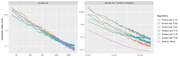
Figure 1: Evolution of the quadratic mean error of the different methods with respect to the sample size (on the left) and to computation time (on the right).

With outliers.

We then introduced an increasing fraction $\delta$ of outliers according to scenarios ($a$), ($b$) and ($d$) described in Section 5.1. We considered samples with size $n=5000$, and estimated the MCM with the help of the Weiszfeld algorithm (indicated by (W)) or with the ASGD (indicated by (R)). We estimated the eigenvalues of the variance with the three proposed methods and with a sample size of $N=2000$ for the Monte-Carlo method before building the variance. For iterative methods, we used $T=50$ iterations.

All robust methods provide accurate estimates of the variance, even in presence of a large fraction of outliers. In addition, one can see that even if Robbins-Monro method is slightly less precise than the other robust alternatives, but performs well any way. Yet, as the Robbins-Monro procedure is less expansive in term of computation time, and because it turns out to be more accurate than the other methods with a same computational budget (see Appendix A.3), this procedure will be preferred for robust mixture models.

	$\delta$ ($\%$)	FixPoint (R)	FixPoint (W)	Gradient (R)	Gradient (W)	Robbins (R)	Robbins (W)	Variance
($a$): $U$	0	0.32	0.24	0.34	0.31	0.45	0.36	0.11
	2	0.39	0.34	0.36	0.34	0.40	0.36	39.75
	3	0.36	0.39	0.39	0.36	0.43	0.38	78.20
	5	0.63	0.51	0.59	0.57	0.57	0.59	212.60
	9	1.35	1.36	1.29	1.21	1.28	1.06	682.80
	16	4.01	3.88	3.91	3.89	3.41	3.36	$2.10^{3}$
	28	16.65	17.56	16.21	16.13	13.78	13.51	$7.10^{3}$
	50	154.52	165.05	133.19	142.32	109.12	116.59	$2.10^{4}$
($b$): $T_{1}$	0	0.31	0.29	0.32	0.34	0.38	0.40	0.10
	2	0.33	0.31	0.30	0.31	0.44	0.37	$2.10^{8}$
	3	0.36	0.28	0.29	0.35	0.40	0.36	$2.10^{7}$
	5	0.35	0.36	0.41	0.40	0.43	0.54	$10^{9}$
	9	0.49	0.46	0.48	0.47	0.67	0.65	$7.10^{9}$
	16	0.86	0.77	0.80	0.76	0.98	0.93	$8.10^{13}$
	28	1.74	1.76	1.64	1.78	2.01	1.92	$5.10^{11}$
	50	5.49	5.28	5.38	5.52	5.59	5.84	$2.10^{13}$
($e$): $T_{2}$	0	0.29	0.28	0.37	0.29	0.46	0.33	0.12
	2	0.33	0.33	0.31	0.34	0.41	0.48	1.06
	3	0.35	0.40	0.42	0.38	0.63	0.41	0.59
	5	0.52	0.60	0.48	0.49	0.66	0.76	7.03
	9	0.86	1.02	0.79	0.98	1.10	1.20	6.10
	16	1.99	2.07	2.08	2.21	2.50	2.54	330.59
	28	5.80	5.59	5.50	5.88	5.92	6.20	$9.10^{6}$
	50	14.84	15.12	14.99	15.16	15.38	15.31	$2.10^{4}$

Table 1: Multivariate Gaussian case: Mean quadratic error of the estimates of the variance for the different methods and for different contamination scenarios and fractions $\delta$.

5.2.2 Student case

We used a similar scheme for the Student distribution.

No outlier.

We considered a Student distribution with null mean vector, with variance $\Sigma_{0}$ and 3 degrees of freedom.

We first focus on the accuracy of each method to estimate the variance and follow the same simulation plan as for the Gaussian case. Observe that in this case, the weighted averaged Robbins-Monro method is slightly less accurate for fixed sample sizes, but is slightly better for fixed computational budget. In Table 2, we first remark that the usual estimate of the variance clearly underperform, even for uncontaminated data. In addition, although gradient method with $50$ iterations is undoubtedly better, the Robbins-Monro alternative is a serious competitor. Then, coupled with what has been observed in the Gaussian case, the method based on the Robbins-Monro algorithm seems the best option for estimating the variances of the clusters of robust mixture models.

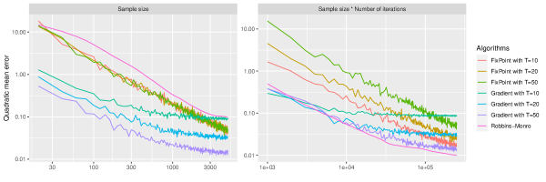
Figure 2: Evolution of the quadratic mean error of the different methods with respect to the sample size (on the left) and to computation time (to the right).

With outliers.

We then introduced an increasing fraction $\delta$ of outliers according to same three scenarios ($a$), ($b$) and ($d$) from Section 5.1.

The conclusion are the same as in the Gausian case.

	$\delta$ ($\%$)	FixPoint (R)	FixPoint (W)	Gradient (R)	Gradient (W)	Robbins (R)	Robbins (W)	Variance
($a$): $U$	0	0.29	0.25	0.20	0.20	0.50	0.46	19.78
	2	0.37	0.36	0.27	0.22	0.46	0.44	43.43
	3	0.41	0.37	0.34	0.27	0.68	0.55	103.51
	5	0.79	0.63	0.62	0.53	1.06	0.84	207.81
	9	2.01	1.82	1.91	1.63	2.34	1.90	733.99
	16	6.73	5.83	6.11	5.61	6.87	6.89	$2.10^{3}$
	28	29.82	27.17	26.84	25.25	30.72	28.27	$7.10^{3}$
	50	393.82	374.55	273.07	260.37	336.28	324.98	$2.10^{4}$
($b$): $T_{1}$	0	0.27	0.26	0.17	0.16	0.38	0.48	16.14
	2	0.37	0.31	0.21	0.17	0.52	0.46	$10^{8}$
	3	0.35	0.27	0.23	0.20	0.52	0.45	$10^{10}$
	5	0.44	0.39	0.31	0.27	0.62	0.69	$3.10^{9}$
	9	0.83	0.75	0.67	0.59	1.22	0.93	$10^{10}$
	16	2.18	1.97	1.90	1.77	2.74	1.98	$2.10^{10}$
	28	6.54	6.17	6.08	5.64	7.00	6.05	$5.10^{12}$
	50	32.39	30.08	29.16	27.99	31.48	29.79	$2.10^{18}$
($e$): $T_{2}$	0	0.30	0.26	0.19	0.18	0.40	0.34	12.77
	2	0.37	0.30	0.21	0.21	0.51	0.45	3.81
	3	0.31	0.32	0.21	0.21	0.42	0.40	9.72
	5	0.33	0.29	0.22	0.22	0.50	0.43	38.64
	9	0.44	0.39	0.34	0.30	0.61	0.59	14.00
	16	0.84	0.80	0.69	0.69	0.98	0.95	778.37
	28	2.08	1.96	1.95	1.91	2.27	2.14	$3.10^{3}$
	50	6.57	6.35	6.56	6.42	7.23	6.45	401.01

Table 2: Multivariate Student case: Mean quadratic error of the estimates of the variance for the different methods and for different contamination scenarios and fractions $\delta$.

5.3 Mixture models

The second part our simulation deals with mixture models.

5.3.1 Gaussian mixture model.

We simulated $B=100$ datasets according to a Gaussian mixture model with each of the parameter configurations described in Section 5.1. We only present here the results for a total sample size of $n=1500$) (that is $n_{k}=500$ observations in each group). We did not observe substantial differences between the results obtained when selecting the number of clusters $K$ with $BIC$ and $ICL$. As a consequence, we only present the results obtained with $BIC$.

The first two columns of Figure 3 compare the results of maximum-likelihood (GMM) inference with the proposed approach (RGMM) in terms of classification. When fixing the number of clusters to its true value $K^{*}=3$, we observe a dramatic drop of the classification accuracy of GMM estimation, even for a very moderate fraction of outliers ($\delta=2\%$), as compared to RGMM, in all scenarios. We observe that estimating the number of clusters with $BIC$ improves the classification performances of GMM, at the price of an increase of the number of clusters. On the contrary, the RGMM approach keeps selecting the right number of clusters, even with a medium fraction of outliers $(\delta\sim 10-20\%)$. As a consequence, model selection does not significantly improve the classification accuracy of RGMM. Lastly, we observe that the difference between GMM and RGMM is even more obvious when outliers can each be associated with one cluster, that is under scenarios ($c$) and ($e$), as opposed to scenarios ($b$) and ($d$), respectively.

	Classification		Parameter estimation
	ARI	$\widehat{K}$	$MSE(\mu)$	$MSE(\Sigma)$
($a$)
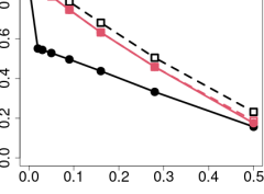
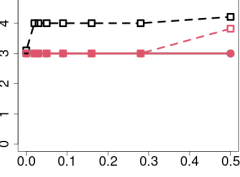
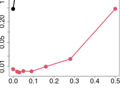
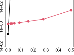
($b$)
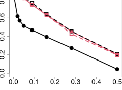
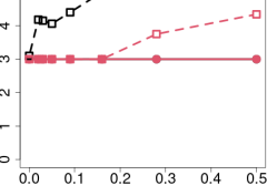
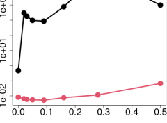
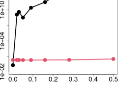
($c$)
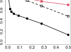
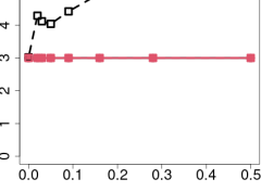
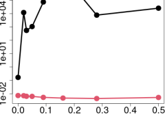
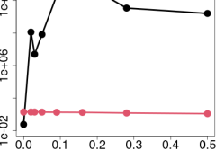
($d$)
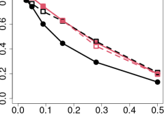
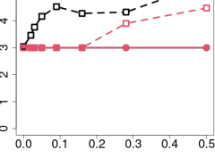
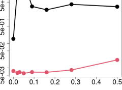
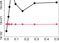
($e$)

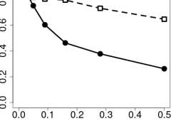
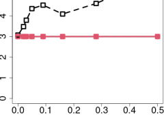
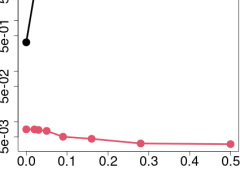
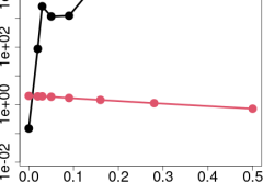
Figure 3: Gaussian mixture model: classification accuracy ($ARI$), estimated number of clusters $\widehat{K}$, estimation error fu the mean ($MSE(\mu)$) and for the variance ($MSE(\Sigma)$) for scenarios ($a$) to ($e$), with $n_{k}=500$ observation in each of the $K^{*}$ clusters ($n=1500$). Black: maximum likelihood (GMM); red: robust estimation (RGMM). Solid line ($\bullet$): with true number of clusters $K^{*}$; dotted line ($\square$): with number of clusters estimated with $BIC$.

The last two columns of Figure 3 compare the respective accuracies of GMM and RGMM in terms of parameter estimation. The precision achieved by RGMM is several order of magnitude better than this of GMM, and, except under scenario ($a$), this accuracy remains the same for large contamination fractions (up to $\delta=50\%$). Again, model selection does not improve the estimation precision of the robust approach.

Figure 5, given in Appendix A.4, is the same as Figure 3, but was obtained with $n_{k}=100$ observations in each cluster (that is $n=300$). The same conclusions, although less contrasted, can be drawn from it.

5.3.2 Student mixture model.

We then simulated $B=100$ datasets according to a Student mixture model with the same set of parameter configurations (see Section 5.1). Again, we only present here the results with $n_{k}=500$ observations in each group ($n=1500$). For the same reason as in the Gaussian case, we only present the results obtained with the $BIC$ criterion.

Figure 4 is organized in the same way as Figure 3. In terms of classification, we observe a dramatic drop of the accuracy obtained with maximum likelihood inference (TMM: as performed by the teigen R package), as compared to its robust counterpart (RTMM). We also observe that, depending on the simulation scenario, the classification accuracy of the robust approach decreases more or less rapidely, the better results being obtained under the scenarios where outliers can each be associated with a clusters (($c$) and ($e$)).

	Classification		Parameter estimation
	ARI	$\widehat{K}$	$MSE(\mu)$	$MSE(\Sigma)$
($a$)
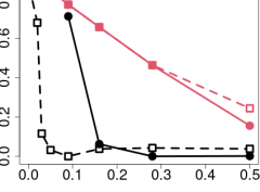
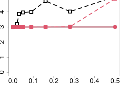
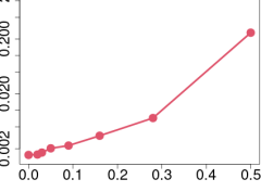
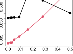
($b$)
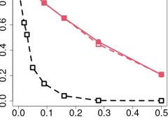
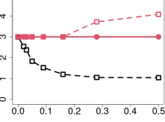
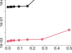
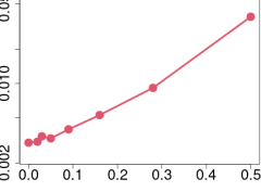
($c$)
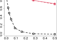
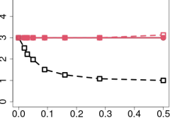
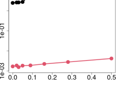
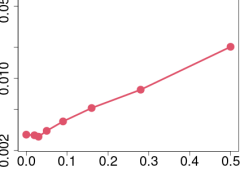
($d$)
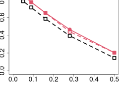
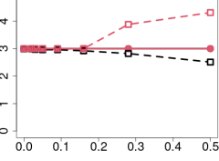
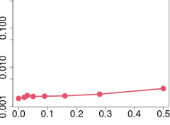
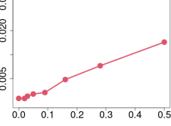
($e$)

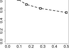
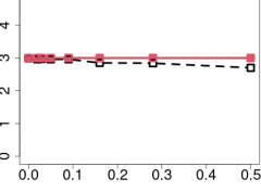
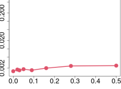
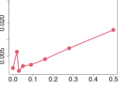
Figure 4: Student mixture model: classification accuracy ($ARI$), estimated number of clusters $\widehat{K}$, estimation error fu the mean ($MSE(\mu)$) and for the variance ($MSE(\Sigma)$) for scenarios ($a$) to ($e$), with $n_{k}=500$ observation in each of the $K^{*}$ clusters ($n=1500$). Same legend as Figure 3.

The last two columns of Figure 4 also shows better performances of the robust approach RTMM as compared to maximum likelihood TMM in terms of precision accuracy. Observe that several curves associated with TMM display an erratic behavior due to convergence issues of the EM algorithm (see Figure 7 in Appendix A.4).

Similarly to de Gaussian case, Figure 6, given in Appendix A.4, is the same as Figure 4 for $n_{k}=100$ observations per cluster ($n=300$): again similar conclusions can be drawn from it.

Aknowledgement.

We are grateful to the INRAE MIGALE bioinformatics facility (MIGALE, INRAE, 2020. Migale bioinformatics Facility, doi:10.15454/1.5572390655343293E12) for providing computing and storage resources.

6 Proofs

Proof of Proposition 1.

Remark that one can rewrite

$$\mathbb{E}_{\theta^{*}}\left[G_{2}(m)\right]=\mathbb{E}_{\theta^{*}}\left[\sum_{k=1}^{K}\mathbf{1}_{Z=k}\left\|X-m_{k}\right\|\right]$$

and this function is Frechet-differentiable with

$$\nabla_{m_{k}}\mathbb{E}_{\theta^{*}}\left[G_{2}(m)\right]=-\mathbf{E}_{\theta^{*}}\left[\frac{X-m_{k}}{\left\|X-m_{k}\right\|}\mathbf{1}_{Z=k}\right].$$

and the zero of the gradient of $G_{2}$ correspond to the median of the classes. Since $X|Z=k$ is symmetric, one has $\nabla_{m_{k}}\mathbb{E}_{\theta^{*}}\left[G_{2}\left(\mu_{k}^{*}\right)\right]=0$, i.e $\mu_{k}^{*}=m_{k}^{*}$. In a same way, one has

$$\nabla_{V_{k}}\mathbb{E}_{\theta^{*}}\left[G_{3}(V)\right] =-\mathbb{E}_{\theta^{*}}\left[\frac{\left(X-m_{k}^{*}\right)\left(X-m_{k}^{*}\right)^{T}-V}{\left\|\left(X-m_{k}^{*}\right)\left(X-m_{k}^{*}\right)^{T}-V\right\|_{F}}\mathbf{1}_{Z=k}\right]$$

and the zero of the gradient correspond to the MCM of the class $V_{k}^{*}$. Then, since $X|Z=k$ is symmetric, the zero of the gradient satisfies $\Sigma_{k}^{*}=\Psi\left(V_{k}^{*}\right)$. ∎

Proof of Proposition 2.

Since $\pi^{*}$ is a zero of the gradient of the Lagrangian, one has $\pi_{k}^{*}=\mathbb{E}\left[\tau_{k}(X)\right]$, i.e one has $\pi^{*}=g_{1}\left(\pi^{*}\right)$. In a same way, $m_{k}^{*}$ is a zero of $\nabla_{m_{k}}G_{2}$, where $\nabla_{m_{k}}$ denotes the partial gradient with respect to $m_{k}$. Furthermore,

$$\nabla_{m_{k}}G_{2}(m) =-\mathbb{E}\left[\tau_{k}(X)\frac{\left(X-m_{k}\right)}{\left\|X-m_{k}\right\|}\right]=0 \Leftrightarrow \mathbb{E}\left[\tau_{k}(X)\frac{X}{\left\|X-m_{k}\right\|}\right] =m_{k}\mathbb{E}\left[\tau_{k}(X)\frac{1}{\left\|X-m_{k}\right\|}\right]$$

$$\Leftrightarrow m_{k} =g_{2,k}\left(m_{k}\right),$$

and in a particular case, $m^{*}$ is a minimizer of $G_{2}$ if and only if $m^{*}=g_{2}\left(m^{*}\right)$. In a same way, denoting by $\nabla_{V_{k}}$ the gradient of $G_{3}$ with respect to $V_{k}$, one has

$$0=\nabla_{V_{k}}G_{3}(m^{*},V) =-\mathbb{E}\left[\tau_{k}(X)\frac{\left(X-m_{k}^{*}\right)\left(X-m_{k}^{*}\right)-V_{k}}{\left\|\left(X-m_{k}^{*}\right)\left(X-m_{k}^{*}\right)-V_{k}\right\|_{F}}\right]$$

$$\Leftrightarrow\quad\mathbb{E}\left[\tau_{k}(X)\frac{\left(X-m_{k}^{*}\right)\left(X-m_{k}^{*}\right)}{\left\|\left(X-m_{k}^{*}\right)\left(X-m_{k}^{*}\right)-V_{k}\right\|_{F}}\right] =V_{k}\mathbb{E}\left[\tau_{k}(X)\frac{1}{\left\|\left(X-m_{k}^{*}\right)\left(X-m_{k}^{*}\right)-V_{k}\right\|_{F}}\right],$$

which concludes the proof.

∎

Appendix A Appendix

A.1 Simulation design

The vectors of means used for the simulation study where the following:

$$\mu_{1}^{\intercal} =[\begin{array}[]{rrrrr}0&0&0&0&0\end{array}], \mu_{2}^{\intercal} =[\begin{array}[]{rrrrr}3&3&3&3&-3\end{array}], \mu_{3}^{\intercal} =[\begin{array}[]{rrrrr}-3&-3&-3&-3&-3\end{array}],$$ (9)

and the variance matrices were

$$\Sigma_{1} =\left[\begin{array}[]{rrrrr}2&0.43&0.41&0.15&0.68\\ 0.43&2&0.7&0.49&0.89\\ 0.41&0.7&2&0.17&0.42\\ 0.15&0.49&0.17&2&0.43\\ 0.68&0.89&0.42&0.43&2\end{array}\right] \Sigma_{2} =\left[\begin{array}[]{rrrrr}1&0.46&0.17&0.04&1.06\\ 0.46&2&0.61&0.18&1.22\\ 0.17&0.61&3&0.7&0.65\\ 0.04&0.18&0.7&4&0.16\\ 1.06&1.22&0.65&0.16&5\end{array}\right]$$ (20)

$$\Sigma_{3} =\left[\begin{array}[]{rrrrr}1&0.6&0.11&0.03&0.26\\ 0.6&0.5&0.09&0.02&0.17\\ 0.11&0.09&0.33&0.03&0.04\\ 0.03&0.02&0.03&0.25&0.01\\ 0.26&0.17&0.04&0.01&0.2\end{array}\right] \Sigma_{0} =\left[\begin{array}[]{rrrrr}4&0.86&0.83&0.29&1.35\\ 0.86&4&1.4&0.97&1.79\\ 0.83&1.4&4&0.35&0.84\\ 0.29&0.97&0.35&4&0.86\\ 1.35&1.79&0.84&0.86&4\end{array}\right]$$ (32)

A.2 Illustration of the results with the R package RGMM

In this Section, we explain how to use the R package RGMM to illustrate the results. First, let us consider the following R code:

> mu <- matrix( c(rep(0,10),rep(2,10),rep(-2,10)), byrow=T, nrow=3)
> ech <- Gen_MM(nk = rep(200,3), delta=0.1,mu=mu)
> X<- ech$X
> Result <- RobMM(X)

The function Gen$\_$MM enables to generate a sample of mixture model (Gaussian, Student or Laplace), whose centers are the raws of the matrix mu. The number of data by cluster is given by nk while delta gives the proportion of contaminated data. The function RobMM gives the results obtained with the help of our method. One can see the vignette for more details and to see the different options.

We now focus on the function RMMplot which enables to illustrate the results. More precisely, we now comment the different available graphics.

> RMMplot(Result,graph=c(’Two_Dim’))

The option ’Two$\_$Dim’ enables to represent the 2 first principal components of the data using robust principal component analysis components (RPCA) (see [Cardot and Godichon-Baggioni, 2015]).

> RMMplot(Result,graph=c(’Two_Dim_Uncertainty’))

The option ’Two$\_$Dim$\_$Uncertainty’ enables also to represent the 2 first principal components, but the size of the points is proportional to the uncertainty of the classification of the data.

> RMMplot(Result,graph=c(’ICL’))
> RMMplot(Result,graph=c(’BIC’))

Options ’ICL’ and ’BIC’ enables to visualize the evolution of the criterion with respect to the number of clusters $K$.

RMMplot(Result,graph=c(’Profiles’))

Option ’Profiles’ allows to visualize data points in dimensions higher than $3$. More precisely, we represent data as curves that we call ”profiles”, gathered it by cluster, and represented the centers of the groups in red.

RMMplot(Result,graph=c(’Uncertainty’))

Option ’Uncertainty’ enables to visualize the uncertainty of classification of the data.

A.3 Additional simulation results for the estimation of the variance

In this section, we provide analogous tables as in Section 5.2, but with analogous calculus budget. More precisely, for gradient and fix point method, we consider a sample size of $N=2000$ for the Monte-Carlo method, while for Robbins-Monro procedure, we consider a sample size of $N=100000$. One can remark that Robbins-Monro procedure provide better results for analogous computational budgets. Nevertheless, the difference is very slight because of the sample size for estimating the MCM is moderate, and the principal error seems to come from this ”bad” estimation.

	$\delta$ ($\%$)	FixPoint (R)	FixPoint (W)	Gradient (R)	Gradient (W)	Robbins (R)	Robbins (W)	Variance
($a$): $U$	0	0.35	0.29	0.36	0.31	0.19	0.18	0.11
	2	0.41	0.37	0.41	0.31	0.21	0.19	34
	3	0.43	0.36	0.37	0.44	0.26	0.24	75
	5	0.67	0.58	0.63	0.57	0.48	0.44	220
	9	1.27	1.25	1.33	1.18	1.13	1.08	690
	16	4.06	3.82	3.89	3.69	3.77	3.70	$2.10^{3}$
	28	17.09	17.53	16.84	16.12	16.84	16.88	$7.10^{3}$
	50	152.32	158.95	128.75	136.53	147.27	153.80	$2.10^{4}$
($b$): $T_{1}$	0	0.27	0.24	0.31	0.27	0.15	0.13	0.09
	2	0.32	0.31	0.32	0.32	0.19	0.17	$3.10^{8}$
	3	0.29	0.29	0.30	0.28	0.17	0.16	$10^{13}$
	5	0.37	0.35	0.33	0.34	0.19	0.18	$10^{12}$
	9	0.46	0.43	0.44	0.43	0.29	0.29	$2.10^{12}$
	16	0.71	0.75	0.81	0.78	0.62	0.61	$3.10^{11}$
	28	1.85	1.85	1.67	1.82	1.62	1.62	$10^{14}$
	50	5.39	5.42	5.48	5.48	5.23	5.19	$10^{11}$
($e$): $T_{2}$	0	0.37	0.33	0.26	0.24	0.15	0.14	0.09
	2	0.38	0.35	0.33	0.33	0.19	0.18	0.10
	3	0.33	0.29	0.33	0.31	0.20	0.19	3.3
	5	0.47	0.54	0.49	0.52	0.34	0.34	45
	9	1.22	0.90	1.03	1.01	0.87	0.89	110
	16	2.04	2.11	2.15	2.14	1.98	2.06	57
	28	5.37	5.67	5.49	5.72	5.46	5.66	810
	50	14.97	15.66	14.90	15.38	15.11	15.31	940

Table 3: Multivariate Gaussian case: Mean quadratic error of the estimates of the variance for the different methods and for different contamination scenarios and fractions $\delta$.

	$\delta$ ($\%$)	FixPoint (R)	FixPoint (W)	Gradient (R)	Gradient (W)	Robbins (R)	Robbins (W)	Variance
($a$): $U$	0	0.25	0.23	0.16	0.15	0.17	0.15	45.82
	2	0.42	0.37	0.30	0.24	0.32	0.24	35.23
	3	0.49	0.39	0.34	0.27	0.36	0.29	285.08
	5	0.75	0.70	0.68	0.59	0.71	0.62	211.14
	9	2.09	1.88	1.82	1.61	1.96	1.72	679.89
	16	7.23	6.20	6.08	5.64	6.59	6.08	$2.10^{3}$
	28	9.36	27.09	26.49	24.74	29.40	27.69	$6.10^{3}$
	50	374.82	363.92	261.54	256.83	371.40	361.54	$2.10^{4}$
($b$): $T_{1}$	0	0.26	0.24	0.19	0.17	0.19	0.17	4.29
	2	0.37	0.27	0.21	0.18	0.21	0.19	$7.10^{11}$
	3	0.36	0.36	0.24	0.21	0.26	0.22	$1.10^{8}$
	5	0.48	0.38	0.30	0.26	0.32	0.27	$6.10^{10}$
	9	0.77	0.75	0.67	0.57	0.70	0.59	$9.10^{10}$
	16	2.17	1.80	1.89	1.69	1.96	1.72	$2.10^{13}$
	28	6.44	6.04	5.99	5.54	6.22	5.82	$7.10^{10}$
	50	30.74	29.61	28.60	27.70	30.85	29.56	$5.10^{14}$
($e$): $T_{2}$	0	0.25	0.27	0.16	0.15	0.17	0.15	8.57
	2	0.28	0.27	0.20	0.18	0.20	0.18	$4.10^{3}$
	3	0.29	0.25	0.20	0.18	0.20	0.18	62.81
	5	0.33	0.33	0.21	0.21	0.22	0.21	5.69
	9	0.43	0.48	0.36	0.34	0.35	0.33	387.11
	16	0.86	0.77	0.68	0.68	0.69	0.65	267.72
	28	1.96	1.92	1.91	1.85	1.90	1.82	164.25
	50	6.66	6.41	6.59	6.48	6.59	6.41	279.53

Table 4: Multivariate Student case: Mean quadratic error of the estimates of the variance for the different methods and for different contamination scenarios and fractions $\delta$.

A.4 Additional simulation results for Mixture models

Figures 3 and 4 provide the simulation results with smaller sample size, namely $n_{k}=100$ observations per clusters, that is $n=300$ observations in total. Figure 5 is the counterpart of Figure 3, and Figure 6 is this of Figure 4.

	Classification		Parameter estimation
	ARI	$\widehat{K}$	$MSE(\mu)$	$MSE(\Sigma)$
($a$)
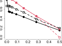
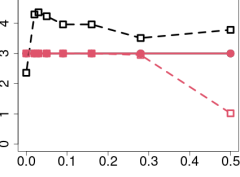
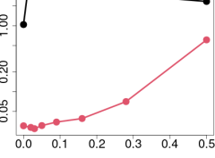
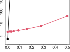
($b$)
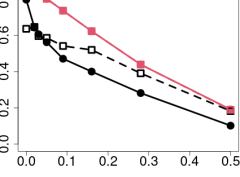
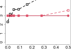
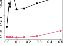
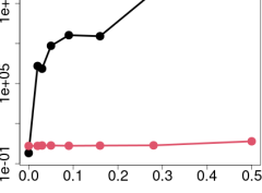
($c$)
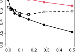
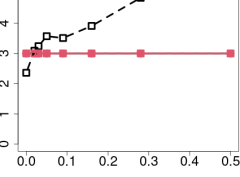
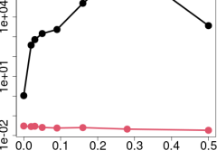
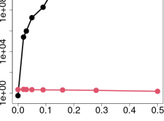
($d$)
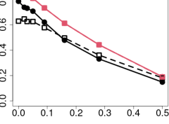
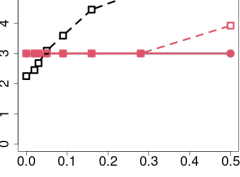
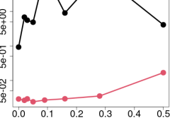
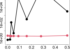
($e$)

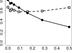
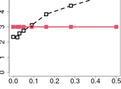
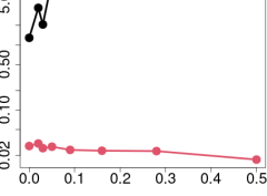
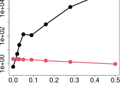
Figure 5: Gaussian mixture model: classification accuracy ($ARI$), estimated number of clusters $\widehat{K}$, estimation error fu the mean ($MSE(\mu)$) and for the variance ($MSE(\Sigma)$) for scenarios ($a$) to ($e$), with $n_{k}=100$ observation in each of the $K^{*}$ clusters ($n=300$). Same legend as Figure 3.

	Classification		Parameter estimation
	ARI	$\widehat{K}$	$MSE(\mu)$	$MSE(\Sigma)$
($a$)
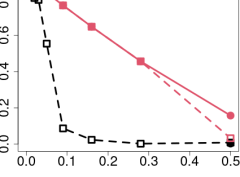
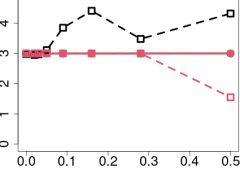
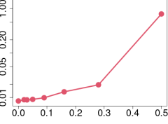
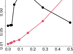
($b$)
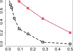
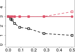
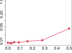
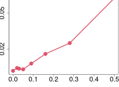
($c$)
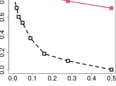
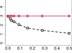
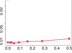
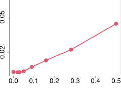
($d$)
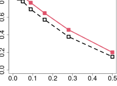
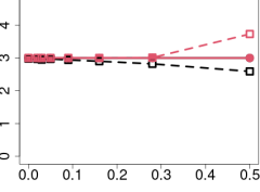
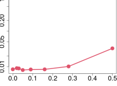
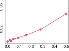
($e$)

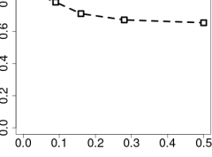
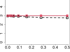
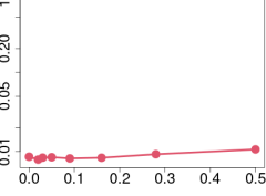
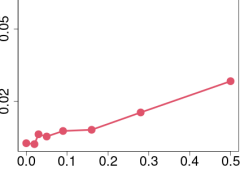
Figure 6: Student mixture model: classification accuracy ($ARI$), estimated number of clusters $\widehat{K}$, estimation error fu the mean ($MSE(\mu)$) and for the variance ($MSE(\Sigma)$) for scenarios ($a$) to ($e$), with $n_{k}=100$ observation in each of the $K^{*}$ clusters ($n=300$). Same legend as Figure 3.

Figure 7 displays the proportion of simulations for which the inference algorithm for the inference of Student mixtures (teigen or RTMM) failed to converge.

($a$)	($b$)	($c$)
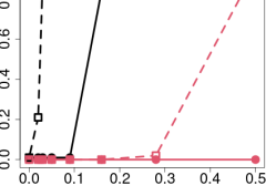
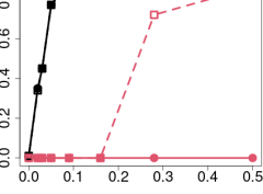
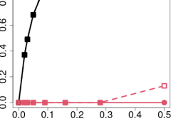
	($d$)	($e$)

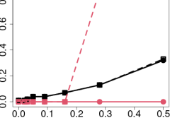
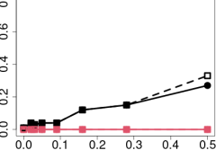
Figure 7: Student mixture model: proportion of non-convergence of the inference algorithms for scenarios ($a$) to ($e$), with $n_{k}=500$ observation in each of the $K^{*}$ clusters ($n=1500$). Same legend as Figure 3. When the number $K$ is estimated (dotted lines), non-convergence that the algorithm did not converge for at least on value of $K$.

References

- [Andrews et al., 2018] Andrews, J., Wickins, J., Boers, N., and McNicholas, P. (2018). teigen: An r package for model-based clustering and classification via the multivariate t distribution. Journal of Statistical Software, 83:1–32.
- [Banfield and Raftery, 1993] Banfield, J. and Raftery, A. (1993). Model-based gaussian and non-gaussian clustering. Biometrics, pages 803–821.
- [Biernacki et al., 2000] Biernacki, C., Celeux, G., and Govaert, G. (2000). Assessing a mixture model for clustering with the integrated completed likelihood. IEEE Trans. Pattern Anal. Machine Intel., 22(7):719–25.
- [Cardot et al., 2017] Cardot, H., Cénac, P., and Godichon-Baggioni, A. (2017). Online estimation of the geometric median in hilbert spaces: Nonasymptotic confidence balls. The Annals of Statistics, 45(2):591–614.
- [Cardot et al., 2013] Cardot, H., Cénac, P., and Zitt, P.-A. (2013). Efficient and fast estimation of the geometric median in Hilbert spaces with an averaged stochastic gradient algorithm. Bernoulli, 19(1):18–43.
- [Cardot and Godichon-Baggioni, 2015] Cardot, H. and Godichon-Baggioni, A. (2015). Fast estimation of the median covariation matrix with application to online robust principal components analysis. TEST, pages 1–20.
- [Coretto and Hennig, 2016] Coretto, P. and Hennig, C. (2016). Robust improper maximum likelihood: tuning, computation, and a comparison with other methods for robust gaussian clustering. Journal of the American Statistical Association, 111(516):1648–1659.
- [Coretto and Hennig, 2017] Coretto, P. and Hennig, C. (2017). Consistency, breakdown robustness, and algorithms for robust improper maximum likelihood clustering. Journal of Machine Learning Research, 18(142):1–39.
- [Dempster et al., 1977] Dempster, A. P., Laird, N. M., and Rubin, D. B. (1977). Maximum likelihood from incomplete data via the EM algorithm. Journal of the Royal Statistical Society: Series B, 39:1–38.
- [Farcomeni and Punzo, 2020] Farcomeni, A. and Punzo, A. (2020). Robust model-based clustering with mild and gross outliers. Test, 29(4):989–1007.
- [Gagolewski et al., 2016] Gagolewski, M., Bartoszuk, M., and Cena, A. (2016). Genie: A new, fast, and outlier-resistant hierarchical clustering algorithm. Information Sciences, 363:8–23.
- [García-Escudero et al., 2008] García-Escudero, L., Gordaliza, A., Matrán, C., and Mayo-Iscar, A. (2008). A general trimming approach to robust cluster analysis. The Annals of Statistics, 36(3):1324–1345.
- [García-Escudero et al., 2010] García-Escudero, L. A., Gordaliza, A., Matrán, C., and Mayo-Iscar, A. (2010). A review of robust clustering methods. Advances in Data Analysis and Classification, 4(2):89–109.
- [Godichon-Baggioni, 2016] Godichon-Baggioni, A. (2016). Estimating the geometric median in hilbert spaces with stochastic gradient algorithms: Lp and almost sure rates of convergence. Journal of Multivariate Analysis, 146:209–222.
- [Gonzalez et al., 2021] Gonzalez, J., Maronna, R., Yohai, V., and Zamar, R. (2021). Robust model-based clustering. Technical Report 2102.06851, arXiv.
- [Gonzalez et al., 2019] Gonzalez, J., Yohai, V., and Zamar, R. (2019). Robust clustering using tau-scales. Technical Report 1906.08198, arXiv.
- [Haldane, 1948] Haldane, J. B. S. (1948). Note on the median of a multivariate distribution. Biometrika, 35(3-4):414–417.
- [Kemperman, 1987] Kemperman, J. (1987). The median of a finite measure on a Banach space. In Statistical data analysis based on the -norm and related methods (Neuchâtel, 1987), pages 217–230. North-Holland, Amsterdam.
- [Kraus and Panaretos, 2012] Kraus, D. and Panaretos, V. M. (2012). Dispersion operators and resistant second-order functional data analysis. Biometrika, 99:813–832.
- [McLahan and Peel, 2000] McLahan, G. and Peel, D. (2000). Finite Mixture Models. Wiley.
- [Mokkadem and Pelletier, 2011] Mokkadem, A. and Pelletier, M. (2011). A generalization of the averaging procedure: The use of two-time-scale algorithms. SIAM Journal on Control and Optimization, 49(4):1523–1543.
- [Peel and McLachlan, 2000] Peel, D. and McLachlan, G. (2000). Robust mixture modelling using the t distribution. Statistics and computing, 10(4):339–348.
- [Polyak and Juditsky, 1992] Polyak, B. and Juditsky, A. (1992). Acceleration of stochastic approximation. SIAM J. Control and Optimization, 30:838–855.
- [Robbins and Monro, 1951] Robbins, H. and Monro, S. (1951). A stochastic approximation method. The annals of mathematical statistics, pages 400–407.
- [Rossell and Steel, 2019] Rossell, D. and Steel, M. (2019). Continuous mixtures with skewness and heavy tails. In Handbook of Mixture Analysis, pages 219–237. Chapman and Hall/CRC.
- [Ruppert, 1988] Ruppert, D. (1988). Efficient estimations from a slowly convergent robbins-monro process. Technical report, Cornell University Operations Research and Industrial Engineering.
- [Schwarz, 1978] Schwarz, G. (1978). Estimating the dimension of a model. The annals of statistics, 6(2):461–464.
- [Scrucca et al., 2016] Scrucca, L., Fop, M., Murphy, B., and Raftery, A. (2016). mclust 5: clustering, classification and density estimation using Gaussian finite mixture models. The R Journal, 8(1):289–317.
-
[Subedi et al., 2015]
Subedi, S., Punzo, A., Ingrassia, S., and McNicholas, P. (2015).
Cluster-weighted
t-factor analyzers for robust model-based clustering and dimension reduction. Statistical Methods & Applications, 24(4):623–649. - [Vardi and Zhang, 2000] Vardi, Y. and Zhang, C.-H. (2000). The multivariate -median and associated data depth. Proc. Natl. Acad. Sci. USA, 97(4):1423–1426.
- [Wang, 2015] Wang, W-Land Lin, T.-I. (2015). Robust model-based clustering via mixtures of skew-t distributions with missing information. Advances in Data Analysis and Classification, 9(4):423–445.
- [Weiszfeld, 1937] Weiszfeld, E. (1937). On the point for which the sum of the distances to n given points is minimum. Tohoku Math. J., 43:355–386.