Adjoint Variable Method for Transient Nonlinear Electroquasistatic Problems

Abstract

Many optimization problems in electrical engineering consider a large number of design parameters. A sensitivity analysis identifies the design parameters with the strongest influence on the problem of interest. This paper introduces the adjoint variable method as an efficient approach to study sensitivities of nonlinear electroquasistatic problems in time domain. In contrast to the more common direct sensitivity method, the adjoint variable method has a computational cost nearly independent of the number of parameters. The method is applied to study the sensitivity of the field grading material parameters on the performance of a 320 kV cable joint specimen, which is modeled as a Finite Element nonlinear transient electroquasistatic problem. Special attention is paid to the treatment of quantities of interest, which are evaluated at specific points in time or space. It is shown that shown that the method is a valuable tool to study this strongly nonlinear and highly transient technical example.

1 Introduction

When developing electrical equipment, engineers optimize initial design proposals by carefully identifying a large number of design parameters. In doing so, they rely on rules of thumb, know-how and previous experience, existing standards and, increasingly, simulation and optimization tools. Numerical optimization is used to simultaneously improve – possibly conflicting – quantities of interest, robustness and costs. While stochastic optimization plays a major role, derivative-based deterministic optimization algorithms are becoming, again, increasingly interesting Ion et al (2018). Their advantages over stochastic methods are a faster convergence, i.e. less expensive optimization runs, and efficient coupling with mesh refinement and reduced order models. However, in case of derivative-based approaches, the problem of efficient gradient computation arises. The most common methods for gradient computation, e.g. finite differences and the direct sensitivity method (DSM), are not well suited for applications with many design parameters because their computational costs scale with the number of parameters Li and Petzold (2004); Nikolova et al (2004). The adjoint variable method (AVM), on the other hand, has computational costs that are almost independent of the number of parameters Li and Petzold (2004); Cao et al (2003); Nikolova et al (2004). The AVM has previously been applied in the analysis of electric networks. The first formulation for the AVM in this context, which was based on Tellegen’s theorem Tellegen (1952), was published by Director and Rohrer Director and Rohrer (1969). Only since the 2000s, the AVM has been applied to electromagnetic problems more often and remains an active field of study Nikolova et al (2004); Georgieva et al (2002); Bakr et al (2014); Park et al (1996); Lalau-Keraly et al (2013); Lee and Ida (2015); Sayed et al (2018). In the field of high voltage (HV) engineering, Zhang et. al. recently used the AVM for topology optimization of a station class surge arrester model with linear media at steady state Zhang et al (2021). However, many HV devices are exposed to transient overvoltages and contain strongly nonlinear materials, so that an investigation of the steady state alone, i.e. in the frequency domain, is not sufficient Hussain and Hinrichsen (2017); Späck-Leigsnering et al (2021a). Therefore, in this work, the AVM is formulated and solved numerically for the nonlinear transient electroquasistatic (EQS) problem. Additionally, a method for sensitivity calculation of QoIs evaluated at a given point in time is presented, since the AVM naturally only considers time-integrated QoIs. The AVM is validated using an analytical example. Subsequently, a nonlinear resistively graded 320 kV high voltage direct current (HVDC) cable joint under impulse operation serves as a prominent technical example. It is shown that the AVM is capable of computing the sensitivities of this highly transient nonlinear problem with reasonable computational effort. This is an important step towards gradient-based optimization of electric devices in HV engineering.

2 Electroquasistatic Problem

The EQS problem in time domain reads

$$-\,\text{div}\left(\sigma\,\text{grad}\left(\phi\right)\right)-\,\text{div}\left(\partial_{t}\left(\varepsilon\,\text{grad}\left(\phi\right)\right)\right) =0 \quad t\in[0,T],\,\,\bm{r}\in\Omega\,{\mathchar 24635\relax\;}$$ (1a)

$$\phi =\phi_{\text{fixed}} \quad t\in[0,T],\,\,\bm{r}\in\Gamma_{\text{e}}\,{\mathchar 24635\relax\;}$$ (1b)

$$-(\sigma\,\text{grad}\left(\phi\right)+\partial_{t}\left(\varepsilon\,\text{grad}\left(\phi\right)\right)\cdot\bm{n} =0 \quad t\in[0,T],\,\,\bm{r}\in\Gamma_{\text{m}}\,{\mathchar 24635\relax\;}$$ (1c)

$$\phi =\phi_{0} \quad t=0\phantom{[,T]},\,\,\bm{r}\in\Omega\,{,}$$ (1d)

where $t$ is the time, $\bm{r}$ is the position vector, $\Omega$ is the computational domain and $T$ is the terminal simulation time. The electric scalar potential is $\phi$. $\sigma$ and $\varepsilon$ represent the electric conductivity and permittivity, respectively. $\phi_{\text{fixed}}$ are the fixed voltages at the electrodes, $\Gamma_{\text{e}}\neq\emptyset$, and $\bm{n}$ is the unit vector at the magnetic boundaries, $\Gamma_{\text{m}}=\partial\Omega\backslash\Gamma_{\text{e}}$. The initial condition is denoted by $\phi_{0}$. In case of a field-dependent conductivity or permittivity, i.e. $\sigma=\sigma(E(\bm{r},t),\bm{r})$ and $\varepsilon=\varepsilon(E(\bm{r},t),\bm{r})$, (1) becomes nonlinear.

The standard two-dimensional (2D) axisymmetric Finite Element (FE) problem of (1) is formulated by discretizing $\phi(\bm{r},t)\approx\sum_{j}u_{j}N_{j}$, where $N_{j}(\bm{r})$ are linear nodal FE shape functions. The degrees of freedom are $u_{j}(t)$, which are assembled in the vector $\mathbf{u}$. The semi-discrete version of (1) according to the Ritz-Galerkin procedure reads

$$\mathbf{K}_{\sigma}\mathbf{u}+\partial_{t}\left(\mathbf{K}_{\varepsilon}\mathbf{u}\right)=0,$$ (2)

with

$$[\bm{K}_{\sigma}]_{ij} =\int_{\Omega}\sigma\,\text{grad}\left(N_{j}\right)\cdot\,\text{grad}\left(N_{i}\right)\,\text{d}\Omega \quad\quad i,j=1,...,N_{\text{N}}\,{,}$$ (3)

$$[\bm{K}_{\varepsilon}]_{ij} =\int_{\Omega}\varepsilon\,\text{grad}\left(N_{j}\right)\cdot\,\text{grad}\left(N_{i}\right)\,\text{d}\Omega \quad\quad i,j=1,...,N_{\text{N}}\,{,}$$ (4)

where $N_{\text{N}}$ denotes the number of nodes. For the time discretization, the implicit Euler time stepping scheme is used. The Newton method is applied in every time step to handle the material nonlinearities.

3 Adjoint Method for Nonlinear EQS Problems

Numerical optimization studies the effects of multiple design parameters, $\bm{p}=[p_{1},...,p_{j},...,p_{N_{\text{P}}}]$, on the QoIs, $G_{k}(\phi,\bm{p})$, $k=1,...,N_{\text{QoI}}$. In each FE simulation, one parameter combination $\bm{p}_{0}$ is adopted, and the QoIs are analyzed by post processing the electric scalar potential. Common design parameters are, in particular, material parameters and the dimensions of the geometry. Taking the cable joint of section 4.2 as an example, possible QoIs are, e.g., the maximum tangential field stress at material interfaces, or the electric losses during impulse operation Späck-Leigsnering et al (2021b); Hussain and Hinrichsen (2017).

The AVM is a method for gradient or sensitivity calculation, which is particularly efficient when the number of parameters, $N_{\text{P}}$, is significantly larger than the number of QoIs, $N_{\text{QoI}}$ Cao et al (2003); Li and Petzold (2004). Sensitivities describe how and how strong a given QoI $G_{k}$ is affected by a design parameter $p_{j}$, i.e.

$$\frac{\text{d}G_{k}}{\text{d}p_{j}}(\bm{p}_{0})=\frac{\partial G_{k}}{\partial p_{j}}(\bm{p}_{0})+\frac{\partial G_{k}}{\partial\phi}\frac{\text{d}\phi}{\text{d}p_{j}}(\bm{p}_{0})\,{,}$$ (5)

where $\bm{p}_{0}$ is the active parameter configuration. In case of nonlinear media, the sensitivity of the electric potential with respect to the parameter, $\frac{\text{d}\phi}{\text{d}p_{j}}$, is typically unknown. The idea of the AVM is to avoid the computation of $\frac{\text{d}\phi}{\text{d}p_{j}}$ by a clever modification of the QoIs Li and Petzold (2004); Cao et al (2003): The QoIs are expressed in terms of a functional $g_{k}$, which is integrated over the temporal and spatial computational domain, $\left[0,T\right]\times\Omega$. Additionally, the nonlinear EQS problem (1) is embedded, multiplied by a test function $w_{k}(\bm{r},t)$, i.e.

$$G_{k}(\phi,\bm{p}) =\int_{0}^{T}\int_{\Omega}g_{k}(\phi,\bm{r},t,\bm{p})\,\text{d}\Omega\,\text{d}t$$ (6)

$$\phantom{=}-\int_{0}^{T}\int_{\Omega}w_{k}(\bm{r},t)\cdot\underbrace{\left(-\,\text{div}\left(\sigma\,\text{grad}\left(\phi\right)\right)-\,\text{div}\left(\partial_{t}\left(\varepsilon\,\text{grad}\left(\phi\right)\right)\right)\right)}_{=0}\,\text{d}\Omega\,\text{d}t\,{.}$$

For any $\phi$ solving (1), the additional term is zero and the test function can be chosen freely. The goal of the AVM is to choose the test function in such a way, that the sensitivity of the extended QoI After a lengthy derivation, it can be shown that the unknown term is eliminated if the test function is chosen as the so-called adjoint variable, i.e. the solution of the adjoint problem Li and Petzold (2004); Cao et al (2003). The adjoint problem for EQS problems with nonlinear materials reads

$$-\,\text{div}\left({\bm{\sigma}_{d}}\,\text{grad}\left(w_{k}\right)\right)+\,\text{div}\left({\bm{\varepsilon}_{d}}\,\partial_{t}\left(\,\text{grad}\left({w_{k}}\right)\right)\right) =\frac{\text{d}g_{k}}{\text{d}\phi}\,{,}\quad t\in[0,T],\,\,\bm{r}\in\Omega\,{\mathchar 24635\relax\;}$$ (7a)

$${w_{k}} =0\,{,} t\in[0,T],\,\,\bm{r}\in\Gamma_{\text{e}}\,{\mathchar 24635\relax\;}$$ (7b)

$$-(\bm{\sigma}_{d}\,\text{grad}\left(w\right)_{k}-\bm{\varepsilon}_{d}\partial_{t}\left(\,\text{grad}\left(w\right)_{k}\right)\cdot\bm{n} =0\,{,} t\in[0,T],\,\,\bm{r}\in\Gamma_{\text{m}}\,{\mathchar 24635\relax\;}$$ (7c)

$${w_{k}} =0\,{,} t=T\phantom{[,0]},\,\,\bm{r}\in\Omega\,{,}$$ (7d)

where all quantities are evaluated at the active parameter configuration $\bm{p}_{0}$. Note the plus sign in front of the term with the time derivative in (7a) instead of the minus sign in (1a) and the terminal condition (7d) instead of the initial condition (1d), which indicate that the adjoint problem needs to be integrated backwards in time or the time reversing variable transformation $\tilde{t}=T-t$ must be applied Cao et al (2002).

The adjoint problem is a linear partial differential equation (PDE) that naturally includes the tensorial material linearizations $\bm{\sigma}_{\text{d}}=\frac{\text{d}\bm{J}}{\text{d}\bm{E}}$ and $\bm{\varepsilon}_{\text{d}}=\frac{\text{d}\bm{D}}{\text{d}\bm{E}}$. Through that, it implicitly depends on the solution of the EQS problem, i.e. $\bm{\sigma}_{\text{d}}(E)$ and $\bm{\varepsilon}_{\text{d}}(E)$. Therefore, in order so solve the adjoint problem in backward mode, the EQS problem must first be solved conventionally, i.e. in forward mode, and its solution stored for all time steps. In case of FE simulations, this can lead to a significant memory overhead Cao et al (2002); Cyr et al (2014). For strategies on how to reduce the memory requirement, see for example Cao et al (2002); Cyr et al (2014).

Once the solution of the electric potential and all adjoint variables, $w_{k}$, are available, all sensitivities can be computed directly by

$$\begin{split}\frac{\text{d}G_{k}}{\text{d}p_{j}}(\bm{p}_{0})&={\int_{0}^{T}\int_{\Omega}\frac{\partial g}{\partial p_{j}}+\,\text{grad}\left(w_{k}\right)\cdot\frac{\partial\bm{J}}{\partial p_{j}}-\,\text{grad}\left(\frac{\partial w_{k}}{\partial t}\right)\cdot\frac{\partial\bm{D}}{\partial p_{j}}\,\text{d}\Omega\text{d}t}\\ &\phantom{=}-\int_{\Omega}\,\text{grad}\left(w_{k}\right)\cdot{\frac{\text{d}\bm{D}}{\text{d}p_{j}}}\,\text{d}\Omega\bigg{|}_{t=0}\,{,}\end{split}$$ (8)

where the derivative ${\frac{\text{d}\bm{D}}{\text{d}p_{j}}}({t=0})$ is obtained by differentiating the initial condition (1d). Again, all quantities are evaluated for the active parameter configuration $\bm{p}_{0}$.

3.1 Finite Element Discretization

The derivative of the electric scalar potential to the parameter $p_{j}$ and the adjoint variable are discretized using linear FE nodal shape functions, i.e.

$$\frac{\text{d}\phi}{\text{d}p_{j}}(\bm{r},t) \approx\sum_{r=1}^{N_{\text{node}}}u^{\prime}_{r}(t)N_{r}(\bm{r}) w(\bm{r},t)\approx\sum_{r=1}^{N_{\text{node}}}w_{r}(t)N_{r}(\bm{r})\,{,}$$

and the time axis is discretized using $N_{t}$ samples, i.e. $t\in\{t_{1}=0,...,t_{n},...,t_{N_{t}}=T\}$. The semi-discrete version of the adjoint problem (7) then reads

$$\bm{K}_{\bm{\sigma}_{d}}\bm{w} -\bm{K}_{\bm{\varepsilon}_{d}}\frac{\text{d}\bm{w}}{\text{d}t}=\bm{q}\,{,}$$ (9)

with

$$[\bm{K}_{\bm{\sigma}_{d}}]_{rs} =\int_{\Omega}\,\text{grad}\left(N_{r}\right)\cdot\bm{\sigma}_{d}\cdot\,\text{grad}\left(N_{s}\right)\,\text{d}\Omega r,s =1,...,N_{\text{N}}\,{\mathchar 24635\relax\;}$$ (10)

$$[\bm{K}_{\bm{\varepsilon}_{d}}]_{rs} =\int_{\Omega}\,\text{grad}\left(N_{r}\right)\cdot\bm{\varepsilon}_{d}\cdot\,\text{grad}\left(N_{s}\right)\,\text{d}\Omega r,s =1,...,N_{\text{N}}\,{\mathchar 24635\relax\;}$$ (11)

$$[\bm{q}]_{r} =\int_{\Omega}\frac{\partial g}{\partial u_{r}}\,\text{d}\Omega r =1,...,N_{\text{N}}\,{.}$$ (12)

Finally, the semi-discrete version for the sensitivity calculation reads

$$\begin{split}\frac{\text{d}G_{k}}{\text{d}p_{j}}(\bm{p}_{0})=&\int_{0}^{T}\int_{\Omega}\frac{\partial g}{\partial p_{j}}\,\text{d}\Omega-\bm{u}^{T}\bm{K}_{\sigma_{p}}w+\bm{u}^{T}\bm{K}_{\varepsilon_{p}}\frac{\partial w}{\partial t}\text{d}t\\ &\phantom{=}+\bm{u}^{T}\bm{K}_{\varepsilon_{p}}\bm{w}\bigg{\rvert}_{t=0}+(\bm{u}^{\prime})^{T}\bm{K}_{\bm{\varepsilon}_{d}}\bm{w}\bigg{\rvert}_{t=0}\,{,}\end{split}$$ (13)

with

$$[\bm{K}_{\sigma_{p}}]_{rs} =\int_{\Omega}\frac{\partial\sigma}{\partial p_{j}}\,\text{grad}\left(N_{r}\right)\cdot\,\text{grad}\left(N_{s}\right)\,\text{d}\Omega r,s =1,...,N_{\text{N}}\,{\mathchar 24635\relax\;}$$ (14)

$$[\bm{K}_{\varepsilon_{p}}]_{rs} =\int_{\Omega}\frac{\partial\varepsilon}{\partial p_{j}}\,\text{grad}\left(N_{r}\right)\cdot\,\text{grad}\left(N_{s}\right)\,\text{d}\Omega r,s =1,...,N_{\text{N}}\,{\mathchar 24635\relax\;}$$ (15)

$$[\bm{q}]_{r} =\int_{\Omega}\frac{\partial g}{\partial u_{r}}\,\text{d}\Omega r =1,...,N_{\text{N}}\,{.}$$ (16)

In the scope of this work, the time integral of (13) is computed using trapezoidal integration and the time derivative in (9) is approximated using the implicit Euler method.

3.2 Treatment of pointwise QoIs

As can be seen from (6), the AVM is naturally suited for integrated QoIs. Often, however, we wish to analyze QoIs that are evaluated at certain points in space or time. The evaluation at a certain position or time can be expressed by Dirac delta functions inside the functional $g_{k}$. To illustrate the effects this has on the AVM, the electric potential evaluated at a specified position $\bm{r}_{\text{ref}}$ and time $t_{\text{ref}}$ is considered as an example, i.e.

$$G_{k}=\int_{0}^{T}\int_{\Omega}g_{k}\,\text{d}\Omega\text{d}t=\int_{0}^{T}\int_{\Omega}\delta(\bm{r}-\bm{r}_{\text{ref}})\delta(t-t_{\text{ref}})\phi\,\text{d}\Omega\text{d}t\,{,}$$ (17)

where $\delta$ is the Dirac delta function. The right-hand side of the adjoint problem is then given by

$$\frac{\text{d}g}{\text{d}\phi} =\delta(\bm{r}-\bm{r}_{0})\delta(t-t_{\text{QoI}})\,{,}$$ (18)

and after discretization in space one finds

$$\bm{q}(t) =\left[\begin{array}[]{ccccccc}0&\ldots&0&1&0&\ldots&0\end{array}\right]^{T}\delta(t-t_{\text{QoI}})\,{.}$$ (20)

In (20), the spatial integration during the derivation of the FE formulation has converted $\delta(\bm{r}-\bm{r}_{0})$ into a unit excitation at the corresponding node. The temporal Dirac function $\delta(t-t_{\text{QoI}})$ on the other hand must be approximated during numeric integration. In the context of this work, this is done by hat functions with an area of one, i.e.,

$$\bm{q}(t_{n})=\left[\begin{array}[]{ccccccc}0&\ldots&0&1&0&\ldots&0\end{array}\right]^{T}\,\frac{1}{\Delta_{\text{imp}}}\delta_{n_{\text{ref}}}^{n}\,{,}$$ (21)

where $\Delta_{\text{imp}}$ denotes the time step size right before and after $t_{\text{ref}}$. The approximation of the Dirac impulse with the help of other functions, e.g. a normal distribution, led to similar results. However, the approximation by a hat function is easy to implement and has the clear advantage of a compact support.

4 Results

In this section, the AVM (7) for transient EQS problems is validated. In the first step, the layered resistor of Fig. 1a is considered, and the FE adjoint and analytic sensitivities are compared. In a second step, the method is applied to a nonlinear 320 kV cable joint specimen and the results are validated using results obtained by the DSM as a reference.

4.1 Analytical Example

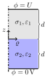
(a)

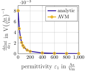
(b)

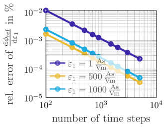
(c)

Figure 1: (a) Resistor with two material layers of thickness $d=1\,$cm. (b) Sensitivity $\frac{\text{d}\phi_{\text{ref}}}{\text{d}\varepsilon_{1}}$ for different values of $\varepsilon_{1}$. (c) Relative error of $\frac{\text{d}\phi_{\text{ref}}}{\text{d}\varepsilon_{1}}$ in % for different numbers of time steps.

The first example is the layered resistor depicted in Fig. 1a. The upper electrode is excited with a sinusoidal voltage, i.e., $U(t)=1\,\text{V}\cdot\text{sin}(\omega t)$ with $\omega=2\pi 50\,\text{Hz}$, and the bottom electrode is grounded. For $t=0$ the potential is assumed to be zero everywhere. The conductivities, $\sigma_{1}=10\,$A/Vm and $\sigma_{2}=20$ A/Vm, and the permittivities, $\varepsilon_{1}=40$ As/Vm and $\varepsilon_{2}=60$ As/Vm, of the two materials are constant. The EQS AVM is validated for an integrated QoI as well as for non-integrated QoI. More specifically, the QoIs are the electrical energy converted in the time span $[0\,\text{s},\frac{2\pi}{\omega}\,\text{s}]$,

$$W_{\text{el}} =\int_{0\,\text{s}}^{\frac{2\pi}{\omega}\,\text{s}}\int_{\Omega}\sigma(\Delta\phi)^{2}\,\text{d}\Omega\,\text{d}t\,{,}$$ (22)

and the potential in the middle of the upper material, i.e., $\bm{r}_{\text{QoI}}=(0,\frac{d}{2})$, evaluated at $t_{\text{QoI}}=\frac{\pi}{2\omega}\,\text{s}$,

$$\phi_{\text{ref}} =\int_{0\,\text{s}}^{2\pi\,\text{s}}\int_{\Omega}\delta(\bm{r}-\bm{r}_{\text{QoI}})\delta(t-t_{\text{QoI}})\phi\,\text{d}\Omega\,\text{d}t\,{.}$$ (23)

First, the sensitivity $\frac{\text{d}\phi_{\text{ref}}}{\text{d}\varepsilon_{1}}$ of the reference potential with respect to the permittivity of the upper material is computed. The time axis is discretized using the step size $\Delta_{\text{main}}$. Directly before and after $t=t_{\text{QoI}}$ the step size is reduced to $\Delta_{\text{imp}}=10^{-8}\Delta_{\text{main}}$ in order to approximate the Dirac impulse. Fig. 1b shows that the AVM is able to reproduce the analytic results of $\frac{\text{d}\phi_{\text{ref}}}{\text{d}\varepsilon_{1}}$ for a wide range of permittivity values. In Fig. 1c a first order convergence of the relative error with respect to the number of time steps can be observed, which matches the order of the implicit Euler method.

Next, the sensitivity $\frac{\text{d}\text{W}_{\text{el}}}{\text{d}\sigma_{1}}$ of the electric energy with respect to the conductivity of the upper material is computed for conductivities ranging from 1 A/Vm to 1000 A/Vm (see Fig. 2a). As shown in Fig. 2b the results again converge linearly with respect to the number of time steps. The AVM has, thus, been successfully validated for a transient EQS problem.

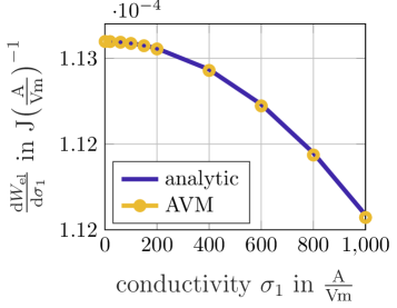
(a)

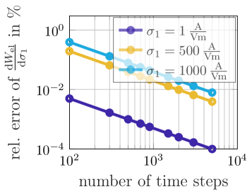
(b)

Figure 2: (b) Sensitivity $\frac{\text{d}\text{W}_{\text{el}}}{\text{d}\sigma_{1}}$ for different values of $\sigma_{1}$. (c) Relative error of $\frac{\text{d}\text{W}_{\text{el}}}{\text{d}\sigma_{1}}$ in % for different numbers of time steps.

4.2 320 kV HVDC Cable Joint Specimen

The development of HVDC cable systems is one of the greatest challenges of our time for the HV engineering community Cigré Working Group D1.56 (2020); Ghorbani et al (2014); Messerer (2022). Cable joints are known to be the most vulnerable part of HVDC systems, as they must safely handle field strengths in the range of several kV/mm Cigré Working Group D1.56 (2020); Chen et al (2015); Jörgens and Clemens (2020); Pöhler and Zhang (2022). The electric field stress can be reduced by adding a layer of so called field grading material (FGM), that features a strongly nonlinear electric conductivity and balances the electric field, similar to the overvoltage clipping of metal-oxide surge arresters Späck-Leigsnering et al (2016, 2021a).

The AVM is applied to a 320 kV HVDC cable joint specimen, which is adopted from Hussain and Hinrichsen (2017) and shown in Fig. 3. The joint connects two copper conductors (domain 1) with an aluminum connector (domain 2). These domains are covered by a layer of conductive silicone rubber (SiR) (domain 3). The cable insulation consists of cross-linked polyethylene (XLPE) (domain 4) and the joint insulation of an insulating SiR (domain 5). Both insulation layers are separated by a nonlinear resistive FGM (domain 6, highlighted in green). The outer conductive SiR sheaths of the cable (domain 7) and the joint (domain 8) are on ground potential. Inside the FGM, elevated field stresses occur at the triple points, i.e., the contact points of FGM, insulating material and conductive SiR (indicated by red circles). The joint is subjected to an impulse overvoltage with an amplitude of $\hat{U}=100\,$kV that is superimposed on the HVDC excitation of 320 kV. The transient standard 1.2/50 lightning impulse is given by Küchler (2017)

$$U_{\text{imp}}(t)=\hat{U}\,\frac{\tau_{2}}{\tau_{2}-\tau_{1}}\,\left(\text{exp}\left(-\frac{t}{\tau_{2}}\right)-\text{exp}\left(-\frac{t}{\tau_{1}}\right)\right)\,{,}$$ (24)

with $\tau_{1}=\frac{1.2\,\upmu\text{s}}{2.96}$ and $\tau_{2}=\frac{50\,\upmu\text{s}}{0.73}$. The excitation is applied to the conductive SiR covering the conductor and the conductor clamp, which is modeled as a perfect electric conductor.

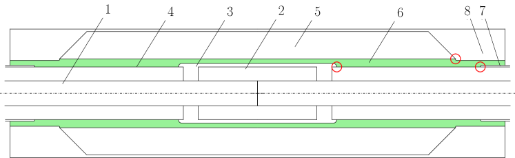
Figure 3: Schematic of the investigated HVDC joint in the $\varrho$-$z$-plane (drawing is not to scale). The typical positions of the maximum tangential field stresses are indicated by red circles Hussain and Hinrichsen (2017). The numbers indicate the different materials as described in the text.

The field-dependence of the conductivity of the FGM is described by the analytic function

$$\sigma(E)=a_{1}\frac{1+a_{4}^{(E-a_{2})\,a_{2}^{-1}}}{1+a_{4}^{(E-a_{3})\,a_{2}^{-1}}}\,{,}$$ (25)

with the parameters $a_{1}=10^{-10}\,\text{A/Vm}$, $a_{2}=0.7\cdot 10^{6}\,$V/m, $a_{3}=2.4\cdot 10^{6}$ V/m and $a_{4}=1864$. The simulation is performed with a mesh consisting of 51681 nodes and 106113 elements.

The results of the EQS AVM are validated against results of the DSM for two exemplary sensitivities. Again, both a time-integrated QoI as well as a QoI evaluated at a specific point in time are considered, i.e., the electric losses, $W_{\text{el}}$, during the time span $[0\,\upmu\text{s},t_{\text{rise}}]$ and the critical electric field stress, $E_{\text{c}}$, in the proximity of the triple point next to the conductor clamp during peak excitation. The derivatives of the QoIs are computed with respect to the switching field strength, $a_{2}$, which determines when the conductivity changes from the base conductivity $a_{1}=10^{-10}$ S/m into the strongly nonlinear region of (25) (see Fig. 4a).

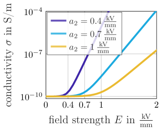
(a)

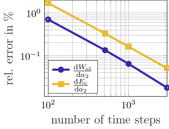
(b)

Figure 4: (a) Field-dependence of the nonlinear conductivity defined for different values of the switching field strength, $a_{2}$. (b) Relative error of $\frac{\text{d}W\text{el}}{\text{d}a_{2}}$ and $\frac{\text{d}E\text{c}}{\text{d}a_{2}}$ for different numbers of time steps in %.

Fig. 4b shows the relative error of the derivatives for different numbers of time steps. A first order convergence due to the Euler time-stepping scheme is observed for both QoIs. More importantly, the computational cost is reasonable for both the time-integrated QoI as well as the QoI evaluated at a given point in time. With only 200 time steps, the relative errors are below one percent, requiring a simulation time in the range of tens of minutes. The AVM was, thus, successfully validated for a strongly nonlinear and highly transient example. It was shown that with the method presented in section 3.2 the AVM is no longer restricted to integrated QoIs. Moreover, it was demonstrated that even for this very challenging example the computation time lies within reasonable limits, which is an important first step towards gradient-based optimization.

5 Conclusion

The adjoint variable method is a method for calculating gradients of selected quantities of interest with respect to a set of design parameters. It has computational costs nearly independent of the number of design parameters and is, thus, very efficient for problems where the number of parameters is larger than the number of quantities of interest. In this work, the adjoint variable method is adopted for transient electroquasistatic problems with nonlinear material characteristics. The adjoint partial differential equation is presented and formulated as a two-dimensional axisymmetric finite element problem. It is shown, how to consider quantities of interest evaluated at specific points in space or time. After validating the method against an analytic example, the method is applied to a 320 kV high voltage direct current cable joint featuring a layer of nonlinear field grading material which is exposed to an impulse overvoltage. The results of the adjoint variable method are validated using the direct sensitivity method and it is shown that the computational costs of the adjoint variable method are, even for this strongly nonlinear technical example, within reasonable limits. This is an important step towards gradient-based optimization of high voltage equipment.

Competing Interests

The authors declare no conflict of interest.

Acknowledgments

The authors thank Rashid Hussain for providing the simulation model and material characteristics published in Hussain and Hinrichsen (2017), and Myriam Koch for the helpful discussions on HVDC cable joints.
This work is supported by the Graduate School CE within the Centre for Computational Engineering at the Technische Universität Darmstadt.

References

- \bibcommenthead
- Bakr et al (2014) Bakr MH, Ahmed OS, Sherif MHE, et al (2014) Time domain adjoint sensitivity analysis of electromagnetic problems with nonlinear media. Optics Express 22(9):10,831. 10.1364/oe.22.010831
- Cao et al (2002) Cao Y, Li S, Petzold L (2002) Adjoint sensitivity analysis for differential-algebraic equations: algorithms and software. Journal of Computational and Applied Mathematics 149(1):171–191. 10.1016/s0377-0427(02)00528-9
- Cao et al (2003) Cao Y, Li S, Petzold L, et al (2003) Adjoint sensitivity analysis for differential-algebraic equations: The adjoint DAE system and its numerical solution. SIAM Journal on Scientific Computing 24(3):1076–1089. 10.1137/s1064827501380630
- Chen et al (2015) Chen G, Hao M, Xu Z, et al (2015) Review of high voltage direct current cables. CSEE Journal of Power and Energy Systems 1(2):9–21. 10.17775/cseejpes.2015.00015
- Cigré Working Group D1.56 (2020) Cigré Working Group D1.56 (2020) Field grading in electrical insulation systems. Technical Brochure TB794. Conseil international des grands réseaux électriques
- Cyr et al (2014) Cyr EC, Shadid J, Wildey T (2014) Towards efficient backward-in-time adjoint computations using data compression techniques. Computer Methods in Applied Mechanics and Engineering 288:24–44. 10.1016/j.cma.2014.12.001
- Director and Rohrer (1969) Director S, Rohrer R (1969) The generalized adjoint network and network sensitivities. IEEE Transactions on Circuit Theory 16(3):318–323
- Georgieva et al (2002) Georgieva N, Glavic S, Bakr M, et al (2002) Feasible adjoint sensitivity technique for EM design optimization. IEEE Transactions on Microwave Theory and Techniques 50(12):2751–2758. 10.1109/TMTT.2002.805131
- Ghorbani et al (2014) Ghorbani H, Jeroense M, Olsson CO, et al (2014) HVDC cable systems—highlighting extruded technology. IEEE Transactions on Power Delivery 29(1):414–421. 10.1109/tpwrd.2013.2278717
- Hussain and Hinrichsen (2017) Hussain R, Hinrichsen V (2017) Simulation of thermal behavior of a 320 kV HVDC cable joint with nonlinear resistive field grading under impulse voltage stress. In: CIGRÉ Winnipeg 2017 Colloquium
- Ion et al (2018) Ion IG, Bontinck Z, Loukrezis D, et al (2018) Deterministic optimization methods and finite element analysis with affine decomposition and design elements. Electrical Engineering 100(4):2635–2647. 10.1007/s00202-018-0716-6
- Jörgens and Clemens (2020) Jörgens C, Clemens M (2020) A review about the modeling and simulation of electro-quasistatic fields in HVDC cable systems. Energies 13(19):5189. 10.3390/en13195189
- Küchler (2017) Küchler A (2017) Hochspannungstechnik: Grundlagen - Technologie - Anwendungen, 4th edn. Springer Berlin Heidelberg, Berlin, Heidelberg, 10.1007/978-3-662-54700-7
- Lalau-Keraly et al (2013) Lalau-Keraly CM, Bhargava S, Miller OD, et al (2013) Adjoint shape optimization applied to electromagnetic design. Optics Express 21(18):21,693. 10.1364/oe.21.021693
- Lee and Ida (2015) Lee HB, Ida N (2015) Interpretation of adjoint sensitivity analysis for shape optimal design of electromagnetic systems. IET Science, Measurement & Technology 9(8):1039–1042
- Li and Petzold (2004) Li S, Petzold L (2004) Adjoint sensitivity analysis for time-dependent partial differential equations with adaptive mesh refinement. Journal of Computational Physics 198(1):310–325. 10.1016/j.jcp.2003.01.001
- Messerer (2022) Messerer F (2022) Current challenges in energy policy. In: HVDC Cable Systems Symposium: Theory and Practice, online, Germany
- Nikolova et al (2004) Nikolova N, Bandler J, Bakr M (2004) Adjoint techniques for sensitivity analysis in high-frequency structure CAD. IEEE Transactions on Microwave Theory and Techniques 52(1):403–419. 10.1109/tmtt.2003.820905
- Park et al (1996) Park IH, Kwak IG, Lee HB, et al (1996) Design sensitivity analysis for transient eddy current problems using finite element discretization and adjoint variable method. IEEE Transactions on Magnetics 32(3):1242–1245. 10.1109/20.497469
- Pöhler and Zhang (2022) Pöhler S, Zhang RD (2022) Prequalification test for extruded 525kV HVDC cable systems – SuedLink and SuedOstLink. In: HVDC Cable Systems Symposium: Theory and Practice, online, Germany
- Sayed et al (2018) Sayed E, Bakr MH, Bilgin B, et al (2018) Adjoint sensitivity analysis of switched reluctance motors. Electric Power Components and Systems 46(18):1959–1968
- Späck-Leigsnering et al (2016) Späck-Leigsnering Y, Gjonaj E, De Gersem H, et al (2016) Electroquasistatic-thermal modeling and simulation of station class surge arresters. IEEE Transactions on Magnetics 52(3):1–4
- Späck-Leigsnering et al (2021a) Späck-Leigsnering Y, Ruppert MG, Gjonaj E, et al (2021a) Simulation analysis of critical parameters for thermal stability of surge arresters. IEEE Transactions on Power Delivery p 1. 10.1109/tpwrd.2021.3073729, DOI: 10.1109/tpwrd.2021.3073729
- Späck-Leigsnering et al (2021b) Späck-Leigsnering Y, Ruppert MG, Gjonaj E, et al (2021b) Towards electrothermal optimization of a HVDC cable joint based on field simulation. Energies 14(10):2848. 10.3390/en14102848, DOI: 10.3390/en14102848
- Tellegen (1952) Tellegen BDH (1952) A general network theorem, with applications. Philips Research Reports 7:256–269
- Zhang et al (2021) Zhang D, Kasolis F, Clemens M (2021) Topology optimization for a station class surge arrester. In: The 12th International Symposium on Electric and Magnetic Fields (EMF 2021)