Conformational degrees of freedom and stability of splay-bend ordering in the limit of a very strong planar anchoring

Abstract

We study the self-organization of flexible planar trimer particles on a structureless surface. The molecules are made up of two mesogenic units linked by a spacer, all of which are modeled as hard needles of the same length. Each molecule can dynamically adopt two conformational states: an achiral bent-shaped (cis-) and a chiral zigzag (trans-) one. Using constant pressure Monte Carlo simulations and Onsager-type density functional theory (DFT), we show that the system consisting of these molecules exhibits a rich spectrum of (quasi-)liquid crystalline phases. The most interesting observation is the identification of stable smectic splay-bend ($S_{SB}$) and chiral smectic A ($S_{A}^{*}$) phases. The $S_{SB}$ phase is also stable in the limit, where only cis- conformers are allowed. The second phase occupying a considerable portion of the phase diagram is $S_{A}^{*}$ with chiral layers, where the chirality of the neighboring layers is of opposite sign. The study of the average fractions of the trans- and cis- conformers in various phases shows that while in the isotropic phase all fractions are equally populated, the $S_{A}^{*}$ phase is dominated by chiral conformers (zigzag), but the achiral conformers win in the smectic splay-bend phase. To clarify the possibility of stabilization of the nematic splay bend ($N_{SB}$) phase for trimers, the free energy of the $N_{SB}$ and $S_{SB}$ phases is calculated within DFT for the cis- conformers, for densities where simulations show stable $S_{SB}$. It turns out that the $N_{SB}$ phase is unstable away from the phase transition to the nematic phase, and its free energy is always higher than that of $S_{SB}$, down to the transition to the nematic phase, although the difference in free energies becomes extremely small when approaching the transition.

I Introduction

Due to their unique shape anisotropy, achiral bent core liquid crystal mesogens can self-assembly in various mesophases, among which the most unusual are the nematic twist-bend phase ($N_{TB}$) Meyer (1976); Cestari et al. (2011); Chen et al. (2013a); Borshch et al. (2013a); Mandle (2016) and the nematic splay-bend ($N_{SB}$) phase Tavarone, Charbonneau, and Stark (2015); Karbowniczek et al. (2017); Karbowniczek (2018). In the $N_{TB}$ phase, there is no long-range positional ordering of the molecules (as in ordinary nematics), but they follow a helix with the average local orientation of the long molecular axis, the director $\mathbf{\hat{n}}(\mathbf{r})$, being tilted with respect to the helical axis. The helical pitch of $N_{TB}$ is on the 10-nanometer scale, and the domains of the left and right induced twists are represented with equal probability. The experimentally observed first-order phase transition from the nematic or isotropic phase to $N_{TB}$ is thus a rare example of spontaneous mirror symmetry breaking. The $N_{SB}$ and the corresponding smectic splay-bend ($S_{SB}$) phases, which will be of our concern here are essentially an in-plane periodic splay-bend modulation of the director, as shown schematically in Fig. 1. In the $S_{SB}$ phase, there is also a quasi-long-range density modulation of molecular centers of mass that coincides with that of the director.

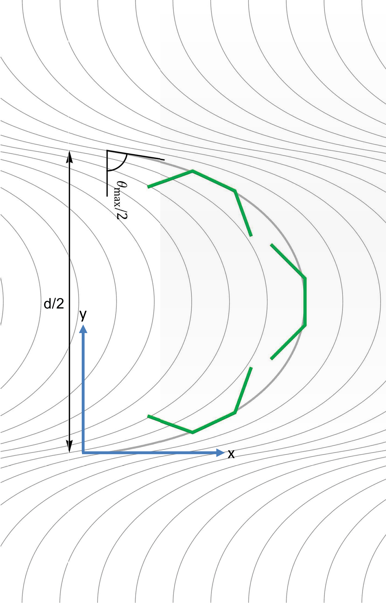
Figure 1: Schematic representation of the periodic splay-bend modulation of the director in $N_{SB}$ and $S_{SB}$. The local director is tangent to the lines (gray) shown and rotates between $\theta_{max}/2$ and $-\theta_{max}/2$ for $0\leq y<d/2$, where $d$ is the period of the structure. Green lines show schematically bent-core molecular conformations that are responsible for the stabilization of the splay-bend ordering.

Modulated nematic structures have been predicted theoretically by Dozov Dozov (2001) who pointed out that molecules whose predominant conformational states are bent ones, should tend to form a spontaneous local bend curvature of $\mathbf{\hat{n}}(\mathbf{r})$. However, unlike the ordinary cholesteric phase, where the three-dimensional (3D) space is filled with a periodic and homogeneous twist de Gennes and Prost (1993), a nematic state of pure spontaneous bend cannot be realized without introducing defects, which are energetically expensive. A less costly, defect-free, periodically modulated bend deformation is also allowed if combined with some twist or splay Meyer (1976); Dozov (2001). The relative stability of these different variants is controlled by the ratio of the splay elastic constant to the twist elastic constant in the underlying nematic phase Dozov (2001); Jákli, Lavrentovich, and Selinger (2018). Uniform periodic bend and twist, where the director simultaneously bends and rotates in the cone, gives the aforementioned $N_{TB}$ phase. Both $N_{TB}$ and $N_{SB}$ must be locally polar by symmetry, and, as it turns out, they do not exhaust the possibilities for stable one-dimensional periodic nematic structures with nonzero bend Longa and Trebin (1990); Longa and Paja̧k (2016); Paja̧k, Longa, and Chrzanowska (2018).

The family of mesogens known to exhibit $N_{TB}$ is quite substantial, obeying (most frequently) chemically achiral dimers Šepelj et al. (2007); Panov et al. (2010); Cestari et al. (2011); Borshch et al. (2013b); Chen et al. (2013b); Paterson et al. (2016); López et al. (2016), bent–core mesogens Görtz et al. (2009); Chen et al. (2014), achiral oligomers Wang et al. (2015); Al-Janabi, Mandle, and Goodby (2017); Mandle and Goodby (2016), or even the recent example of a hydrogen-bonded complex Jansze et al. (2015). In contrast, the $N_{SB}$ phase is scarce. It has been observed in colloidal bananas Fernández-Rico et al. (2020), but not, to our knowledge, in bulk thermotropic materials. However, a transition $N_{TB}$ to $N_{SB}$ can be induced by an applied electric field Paja̧k, Longa, and Chrzanowska (2018); Merkel et al. (2018); Meyer et al. (2020), or as an interface between two homochiral $N_{TB}$ domains of opposite chiralities Meyer, Luckhurst, and Dozov (2015). It is not clear why the bulk $N_{SB}$ has not been detected so far, given the hundreds of mesogens with $N_{TB}$. According to Dozov’s theoryDozov (2001) the ordering $N_{SB}$ can spontaneously form if the splay elastic constant is less than twice the twist elastic constant, which seems to be in favor of at least some of the experimental data Yun et al. (2015); Babakhanova et al. (2017). Recently, using Monte Carlo simulations and mesoscopic modeling, it has been demonstrated that the limitations of stabilizing $N_{SB}$ can be circumvented in some cases if we confine bent core molecules to a planar surface Tavarone, Charbonneau, and Stark (2015); Karbowniczek et al. (2017); Karbowniczek (2018). Here, the $N_{SB}$ phase can win over $N_{TB}$ because development of twist deformations, which require a kind of an ”escape into 3D”, is hampered by the imposed constraints.

Clearly, none of the molecules that self-organize in $N_{TB}$ has a fixed geometry, and the population of conformational molecular states, which is governed by a dynamic equilibrium, can be important (see e.g. Archbold et al. (2017) and references therein). Here, we study this effect on the formation of a stable splay-bend, nematic, and smectic orderings. Since, to date, the most probable scenario for obtaining stable splay-bend modulation is spatial confinement Meyer, Luckhurst, and Dozov (2015), or an external field Paja̧k, Longa, and Chrzanowska (2018); Merkel et al. (2018); Meyer et al. (2020) we limit ourselves to a monolayer composed of molecules with conformational degrees of freedom.

We generalize our two-segment hard V-shaped molecules Karbowniczek et al. (2017); Karbowniczek (2018) to three segments of equal length (trimers), where the side ones are allowed to occupy different conformational states. Even in this simple model, the inclusion of conformations can be realized in many different ways (see e.g. Józefowicz and Longa (2007)). Here, we limit ourselves to the simplest possibility, where for each equivalent side segment of the molecule only two conformational states are allowed, as shown in Fig. 2. This leads to four conformations per molecule, where the non-chiral bent ones (cis+,cis-), Fig. 2 (b, c), are expected to support stable splay-bend deformations Tavarone, Charbonneau, and Stark (2015); Karbowniczek et al. (2017); Karbowniczek (2018), while the chiral (zigzag-, zigzag+) ones, Fig. 2 (a,d), are in favor of mirror symmetry breaking. In addition to the main aim of this work related to stabilization of splay-bend and related orderings, taking chiral conformers into account can contribute to our understanding of the problem of spontaneous mirror symmetry breaking in monolayers composed of flexible achiral mesogens, especially whether it is driven by flexopolarization Meyer (1976); Dozov (2001); Vaupotič et al. (2014) or some other mechanism Lubensky and Radzihovsky (2002); Goodby (2017). These studies should also be of importance in modeling the trans-cis isomerization that occurs when photo-switchable molecules are attached to a surface Delaire and Nakatani (2000); Katsonis et al. (2007); Browne and Feringa (2009); Fang et al. (2010); Wu et al. (2021)

We should add that, so far, zigzag+ and cis+ trimer particles subjected to planar confinement have been considered separately i.e. without conformational degrees of freedom. More specifically, for purely zigzag+ trimer molecules, Pe’on et al. Peón et al. (2006) showed the possibility of stable nematic and smectic phases. The Onsager-type theory for this system was later developed by Varga et al. Varga et al. (2009), leading to similar predictions for liquid crystalline structures. By systematic manipulation of the shape anisotropy, they found that the zigzag- shape with increasing bending angle and length of the side molecular segments favors the smectic order relative to the nematic one. Interestingly, in the smectic layers, the central segment of the trimer zigzag+ was tilted with respect to the layer normal, and each layer behaved like an ideal gas of trimers (on average) with parallel orientation.

The study of cis+ trimers in 2D was initially carried out by Martinez et al. J. Martínez-González (2012). The authors found a quasi-long-range nematic and tetratic order, a curly nematic pattern similar to that of $N_{SB}$ (or $S_{SB}$), and the formation of chiral clusters despite the fact that the particles were achiral. All these works have been refined next by Tavarone et al. Tavarone, Charbonneau, and Stark (2015), where the authors quantified the difference in the thermodynamic behavior of the two molecular geometries. In addition to the Monte Carlo simulations in different ensembles, they implemented a more advanced Monte Carlo algorithm involving cluster moves to find evidence for the splay-bend deformations and to demonstrate that the isotropic quasi-nematic transition observed follows a Kosterlitz-Thouless disclination unbinding scenario. They also used a simplified version of Onsager’s Density Functional Theory to explain some of their results, such as the observed quasi-nematic–quasi-smectic phase transition.

The model presented here that combines the properties of both types of particles is a generalization of the studies mentioned above. Although this system seems interesting in itself, our choice is also motivated by the recent work of Jansze et. al.Jansze et al. (2015) on $N_{TB}$ driven by hydrogen bonding in systems based on benzoic acid. The authors attribute the stabilization of the $N_{TB}$ phase to the formation of cyclic hydrogen-bonded supramolecular trimers, similar to our bent (cis) conformers. These trimers coexist in dynamical equilibrium with open hydrogen-bonded complexes, which, in turn, are similar to chiral (zigzag) conformers and monomers (which are not present in our simplistic model).

An interesting question then is whether our simplified model, which also entails dynamical equilibrium trans-cis subjected to confined geometry, can stabilize the splay-bend ordering (in analogy to the one observed in Meyer, Luckhurst, and Dozov (2015)) and perhaps some other quasi-liquid crystalline structures. To examine such property-structure correlations, we will carry out Monte Carlo simulations at constant pressure for a monolayer composed of $500\leq N\leq 2000$ molecules shown in Fig. 2 along with an Onsager Density Functional analysis. The paper is organized as follows. Section II defines the model that is next studied in Section III using Monte Carlo simulations at constant pressure. The results of the simulations are further supported by predictions of Onsager’s DFT formalism in Sections IV and V. The last section provides a brief summary along with the main conclusions.

II Model Particles

We study a simple athermal model of hard flexible molecules whose positions and orientations are limited to a structureless planar surface or, equivalently, to be subjected to a strong planar anchoring. Each molecule is made up of three segments of the same length $l=1$, with flexible arms attached to the central one. Arms can adopt two conformational states: achiral bent (cis$\pm$ ) and chiral (zigzag$\pm$) parameterized by dynamic variables $s_{\beta i}=\pm 1$, with $\beta$ labeling the arms of the $i-th$ molecule (Fig. 2). The relative orientation of the arm to the central segment is given by a single angle $\alpha$. In the limiting case of $\alpha=0$, the molecule is reduced to a needle of length 3. The relative population of the conformes is governed by purely excluded volume interactions and a given fixed pressure or density.

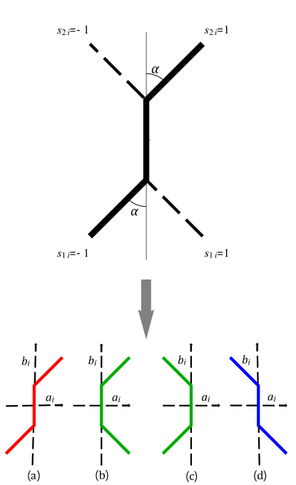
Figure 2: Parametrization of particle’s conformational degrees of freedom (top) and resulting four conformers (bottom). Particles are build out of three segments of the same length $l=1$. Each side segment can independently and with equal probability orient at angle $\pm\alpha$ with respect to the central segment, which we parameterize using two discrete variables ${s_{ji}}=\pm 1;\,\,j=1,2$. Four resulting conformers are: bent (equiv. cis$\pm$) conformations (b,c) and chiral zigzag$\mp$ (equiv. trans$\mp$) conformations (a,d). Note that (b) and (c) differ by the $\pi$-rotation while (a) and (d) are of opposite chirality in 2D. In simulations and DFT calculations we use local, molecule-attached orthogonal system with $b_{i}$ axis kept parallel to the central molecular segment and $a_{i}$ axis perpendicular to it. The $\{a_{i},b_{i}\}$ axes cross in the mid-point of the central segment.

As mentioned above, monolayer studies to date indicate that bent molecular architectures should support stable splay-bend-type deformation Tavarone, Charbonneau, and Stark (2015); Karbowniczek et al. (2017); Karbowniczek (2018). Therefore, adding conformations that preserve bent is not expected to qualitatively change this picture, and in our elementary model, we represent all possible bent conformations (see Fig. 2) by a single (averaged) bent shape. The addition of zigzag conformations of opposite chiralities should favor smectic ordering and mirror symmetry breaking. However, it is of interest to observe the entropic competition between these two effects on the phase sequence. To identify stable structures and their properties and locate phase boundaries, we performed NPT Monte Carlo simulations at a constant number of particles (N), constant pressure (P), and constant temperature (T), supported by Onsager density functional theory and bifurcation analysis. We limit ourselves to sampling molecular translational, orientational, and conformational states. The kinetic energy part of the partition function is integrated over momenta. For the $i-th$ particle, it leads to a factor, say $\Lambda({s_{1i},s_{2i}},T)$, which depends on the conformational degrees of freedom $s_{\alpha i}$ Józefowicz and Longa (2011). To keep our model as simple as possible and to avoid parameters that are difficult to control, we disregarded the conformers’ energy landscape. In the same spirit, we replace $\Lambda({s_{1i},s_{2i}},T)$ by its average value $\overline{\Lambda(T)}$, where the average is taken over the degrees of freedom of the molecular conformations. With this assumption, the average number of conformers in a given structure is governed exclusively by the packing entropy. Therefore, in the reference isotropic phase, at least at low densities, their average fractions should be the same.

III Monte Carlo results

Monte Carlo simulations were performed in an NPT ensemble. The system consisted of particles $N=500$ to $N=2000$ in a square box with side length $L$ and periodic boundary conditions applied. In the MC cycle, we probed a new configuration for randomly chosen N molecules. A trial molecular configuration was generated by a random move of the center of mass of the molecule, a random rotation of the local molecular frame and with the probability of $0.1$ a random change in molecular shape by choosing one of the four possible conformations (see Fig. 2) with the same probability. The step was accepted if the particle did not intersect with the others. After every ten cycles, the size of the box was adjusted to keep the pressure constant. Rescaling kept the box square. In simulations 40% to 50% of new molecular configurations, system rescaling and conformational changes were accepted. Lower acceptance ratios were used for dense and highly ordered states, allowing the solution to partially overcome metastability traps. The reduced density was calculated as

$$\bar{\rho}=Nl^{2}/S\equiv N/S,$$ (1)

where $S=L^{2}$ is the surface area and the length $l$ of the molecular segment is $l=1$. Each simulation was initialized from a random, disordered gas of conformers within a large box, and the pressure was increased in adjustable steps until the transition to (quasi-)liquid crystalline phases occurred. The equilibration appeared slow and took about $2.5\cdot 10^{6}$ cycles, after which the data were collected for the analysis of the structure once per 10 cycles in a production run of $10^{4}$ cycles. To verify that the equilibrated configurations were not just metastable states, we used different initial states, including perfectly oriented polar and antipolar nematic/smectic configurations.

Interestingly, we observed five distinct liquid phases: isotropic ($I$), nematic ($N$), $S_{SB}$, smectic A with chiral layers of alternating chirality ($S_{A}^{*}$), in which both types of particles are tilted relative to each other, and coexisting domains with different local order, which we denoted as $M$. Typical configurations of ordered structures are presented in Fig. 3. Color coding is used for different conformers: red and blue for chiral zigzag and green for achiral bent core ones (cis), respectively.

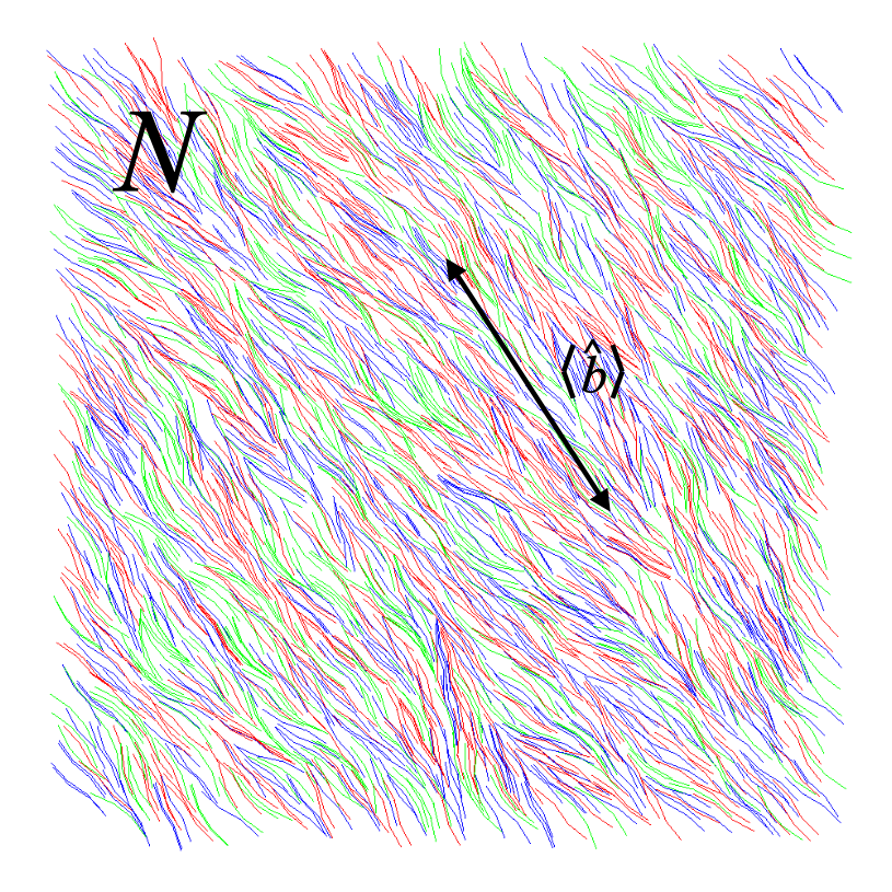
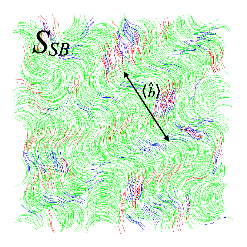
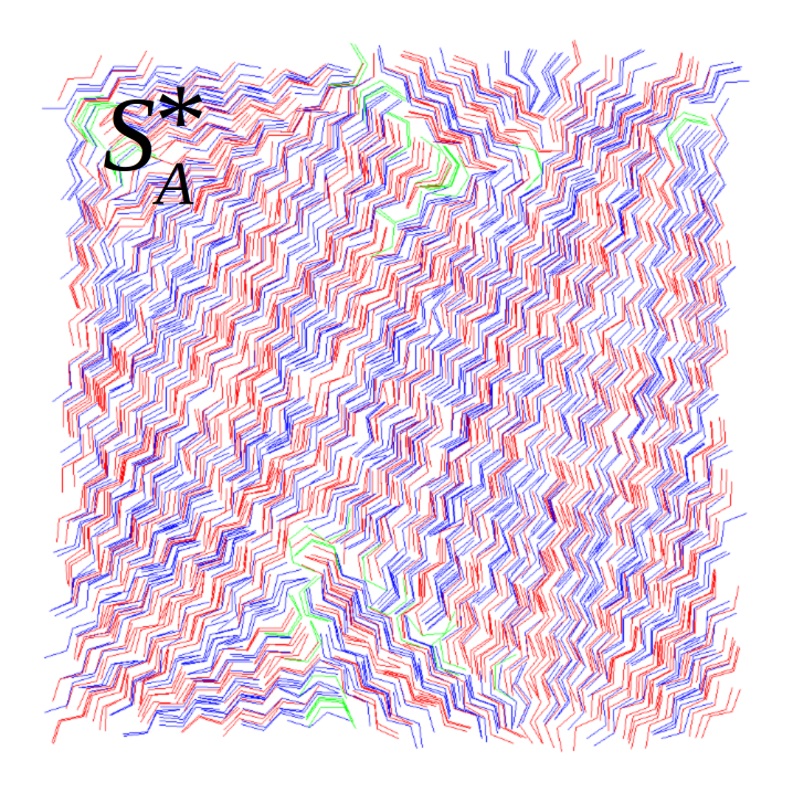
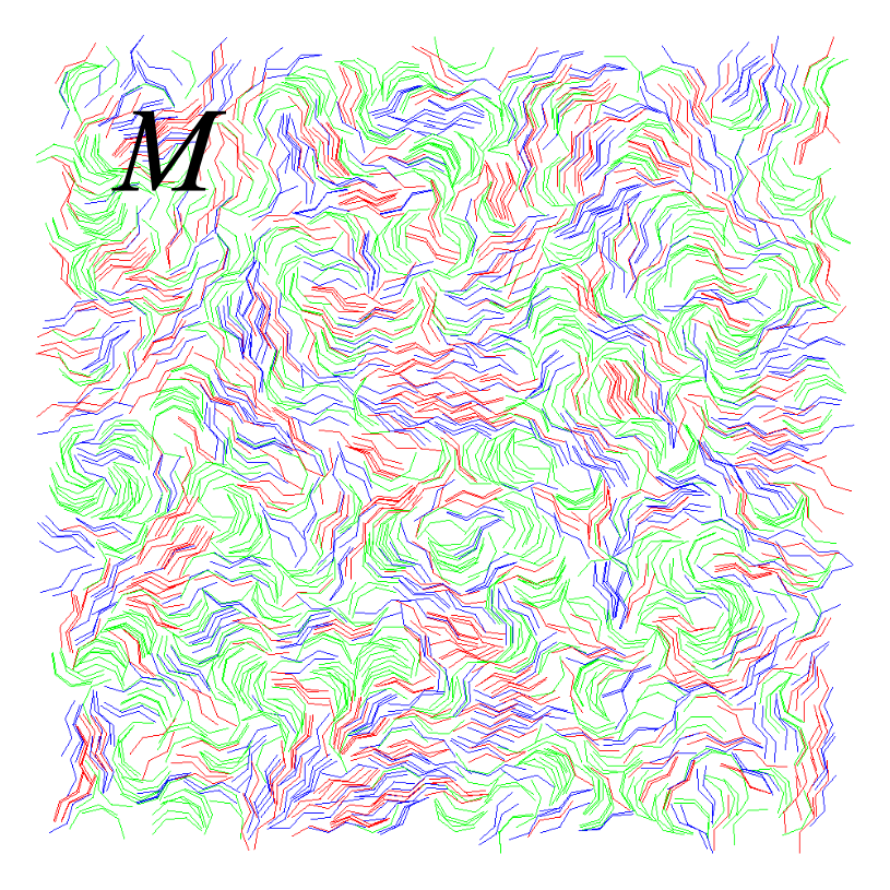
Figure 3: Examples of ordered structures found in simulations: nematic ($N$) for $\alpha=\pi/12$ and $\bar{\rho}=2.0$, smectic splay-bend ($S_{SB}$) for $\alpha=\pi/6$ and $\bar{\rho}=3.1$, and (antichiral) smectic A ($S_{A}^{*}$) for $\alpha=\pi/3$ and $\bar{\rho}=2.5$; $\langle\mathbf{\hat{b}}\rangle=\langle\frac{1}{N}\sum_{i=1}^{N}b_{i}\rangle$ stands for the average orientation of the central molecular segments. The last picture presents a mix ($M$) of differently ordered domains ($\alpha=\pi/4$, $\bar{\rho}=1.39$). In isotropic and nematic phases fractions of red and blue conformers (Fig. 2) are statistically the same. In $S_{SB}$ achiral conformers dominate, and in $S_{A}^{*}$ they disappear. Color coding is used to distinguish between different conformers (see caption to Fig.2).

The fractions of different conformers change from phase to phase. In general, the cis conformers disappear with increasing density. In a well-established $S_{A}^{*}$ phase, where the average main axis of the inertia tensor of the zigzag conformers remains parallel to the layer normal, there are almost no achiral cis conformers. The only exception to this behavior was found in the $S_{SB}$ phase. In that case, a small fraction of the zigzag conformers is located between the splay-bend layers (see the upper right panel of Fig. 3). The dependence of the fractions of the achiral cis conformers on the packing density for the transitions $I-S_{SB}$ and $I-S_{A}^{*}$ is shown in Fig. 4.

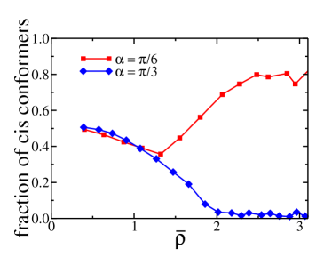
Figure 4: Dependence of density on pressure (left) and fraction of cis conformers (the green one in Fig. 3) on density (right) for $\alpha=\pi/6$ and $\alpha=\pi/3$.

Note that there are no discontinuities in this dependence and in the dependence of the density on the pressure. Therefore, to quantitatively distinguish the observed structures, we use the bond correlation function $g_{2}(r)$:

$$g_{2}(r)=\left\langle\frac{\sum_{i=1}^{N}\sum_{j=i+1}^{N}P_{2}\left(\boldsymbol{u}_{i}\cdot\boldsymbol{u}_{j}\right)\delta\left(r-r_{ij}\right)}{\sum_{i=1}^{N}\sum_{j=i+1}^{N}\delta\left(r-r_{ij}\right)}\right\rangle$$ (2)

since it is a well-established method of phase differentiation (see, for example, Tavarone, Charbonneau, and Stark (2015); Cinacchi et al. (2017); Schlotthauer et al. (2015)). Exemplary correlations $g_{2}(r)$ are presented in Fig. 5. The transition from $I$ to $N$ and the subsequent transition to smectics occur along with the increase in the correlation length. In the smectic phases, there are also visible peaks in the $g_{2}(r)$ function that indicate density modulation along the propagation of the wave vector. However, when the transition to $S_{SB}$ occurs, there is a significant reduction in the correlation length, due to the period of the splay-bend slabs formed.

Using $g_{2}(r)$ and abrupt changes in the average conformer population as a transition indicator, we constructed the phase diagram of our system, Fig. 6. We observed $I-N-S_{SB}$ and direct $I-S_{A}^{*}$ phase transitions as a function of density. Furthermore, the coexisting domains of $N$, $S_{SB}$, and $S_{A}^{*}$ were identified and denoted $M$. This mix of phases appeared independently in the starting configuration for the MC simulations; we tried all: $I$, $N$, $S_{SB}$, and $S_{A}^{*}$ as initial configurations, and in all cases we end up with the $M$ phase. Similarly, we checked the stability of the remaining phases.

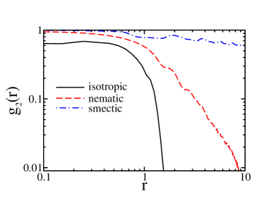
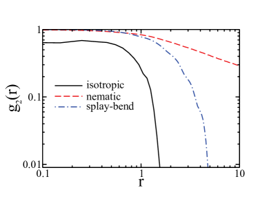
Figure 5: Examples of bond-order correlations. The plot on the left corresponds to $\alpha=60^{\circ}$. The solid black line was obtained for $\bar{\rho}=0.4$ and corresponds to the isotropic phase. The dashed red line is for $\bar{\rho}=1.5$ and is typical for nematics, while the blue dashed line ($\bar{\rho}=2.5$) shows quasi-smectic ordering. For $\alpha=30^{\circ}$ (right panel), the red dashed line ($\bar{\rho}=1.6$) corresponds to the nematic phase and the blue dashed line ($\bar{\rho}=3.1$) corresponds to the smectic splay-bend order.

As expected, for low densities, the isotropic phase is observed. For higher densities, the behavior of the system depends on the angle $\alpha$. When it is small, only the nematic phase stabilizes. For higher values of $\alpha$, up to $\alpha<2\pi/9$, the high-density phase is $S_{SB}$. When $\alpha>2\pi/9$, it is replaced by $S_{A}^{*}$. The background color of the phase diagram corresponds to the fraction of cis conformers. Bow-shaped conformers dominate only in the $S_{SB}$ phase. In the $N$ and $S_{A}^{*}$ phases, this type of conformer disappears with density growth.

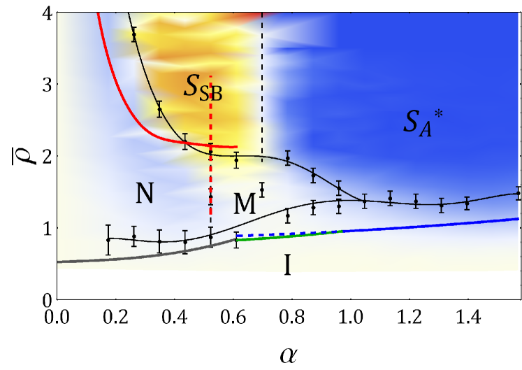
Figure 6: Phase diagram obtained from Monte Carlo simulations and DFT analysis. Background colorization, corresponding to the fraction of cis conformers, is explained in the horizontal legend. Blue color corresponds to the domination of trans particles, whereas red/yellow for $cis$ ones. Thin lines with error bars correspond to data from MC simulations. Solid thick lines are obtained from Onsager’s DFT analysis as explained in the body of the paper. These lines correspond to the transitions from the isotropic phase to nematic (dark grey), mixed phase (green) and smectic A (blue line) phases using analysis with full orientational degrees of freedom. The blue line is extended to the mixed phase region and presented as a dashed line in order to help to explain complicated behaviour in this phase further in the text. Thick red line corresponds to the transition from ideally oriented nematic to splay-bend phase. Along dashed red line a full numerical solution of DFT is obtained for cis particles (see Section IV).

Finally, we also checked the profile of director’s orientation $\theta(y)$ in the splay-bent layer. This dependence has to be assumed prior to any analytic calculations based on density functional theory. In previous studies, several different profiles were used. To obtain the profile, we extracted a single layer from the snapshot taken for $\alpha=\pi/6$ and $\bar{\rho}\approx 3.0$, where the $S_{SB}$ phase dominates. Then, the dependence of the average orientation of a particle on its distance from the center of the layer was measured. The results are shown in Fig.7.

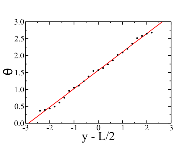
Figure 7: Dependence of the mean particle orientation on its distance from center of a splay-bent layer. Results were calculated for a single layer taken from the system described by $\alpha=\pi/6$ and $\bar{\rho}\approx 3.0$. The black dots are the measured data and the red solid line is the linear fit: $\theta=\pi/2+0.54353\cdot(y-L/2)$, where $y-L/2$ is the distance from the layer’s center.

For the width of the layer here to be slightly less than $5.0$, the director orientation profile is fairly well approximated by the linear function. Furthermore, the direction of the director in a single layer does not cover the full possible spectrum of angles $(0,\pi]$, but is limited to $[0.15\pi,0.85\pi]$. It indicates in a very high orientational order in $S_{SB}$, with the director rotating between $\pm\theta_{max}/2$ (Fig. 1) as we proceed along the $y-$ axis.

IV Density Functional analysis

Following our previous work Karbowniczek et al. (2017), to identify stable structures and their properties and locate phase boundaries, we supplemented computer simulations with analysis based on Onsager-like density functional theory (DFT). We start with a brief summary of the Onsager formalism for our model, see Fig.2. Neglecting the external field terms, the Onsager non-equilibrium free energy functional, $\mathcal{F[\rho]}$, for a system of molecules with conformational degrees of freedom subjected to planar confinement is given by

$${\beta\mathcal{F}\left[\rho\right]} = ~{}\underset{(X)}{Tr}\left\{\rho(X)\left[\,\ln\left(\overline{\Lambda(T)}\rho(X)\right)-1\right]\right\}-\frac{1}{2}\underset{(X_{1},X_{2})}{Tr}\left[\rho(X_{1})f_{12}\,\rho(X_{2})\right],$$ (3)

where $f_{12}=e^{-\beta V(X_{1},X_{2})}-1$ stands for the Mayer function, $V(X_{1},X_{2})$ is the interaction potential, $\beta=\frac{1}{k_{B}T}$ is the reduced temperature with $k_{B}$ being the Boltzmann factor, and $\rho(X)$ is the local particle density routinely normalized to the total number of molecules:

$${Tr}_{(X)}\rho(X)=N.$$ (4)

The variable $X_{i}\equiv\{{\mathbf{r}_{i}},\theta_{i},\mathbf{s}_{i}\}$ ($X\equiv\{{\mathbf{r}},\theta,\mathbf{s}\}$) represents the translational, orientational, and conformational degrees of freedom of the molecule ’$i$’, where $\mathbf{r}_{i}=(x_{i},y_{i})$ is the position of the center of the central molecular segment of the particle, and $\mathbf{s}_{i}=(s_{1i},s_{2i})$ parameterizes the molecular conformational degrees of freedom with $s_{\beta i}=\pm 1$ and $\beta=1,2$. The molecular orientation, given by the angle $\theta_{i}$, is measured between the central molecular segment (parallel to the $b_{i}$ axis of the molecule-fixed frame $\{a_{i},b_{i}\}$, denoted by the dashed thin line in Fig. 2) and the $y-axis$ of the laboratory reference frame and

$${Tr}_{(X_{i})}=\sum_{s_{1i}=\pm 1,\>s_{2i}=\pm 1}\int_{0}^{L}dx_{i}\int_{0}^{L}dy_{i}\int_{-\pi}^{\pi}d\theta_{i}.$$ (5)

For hard-core interactions, the Mayer function is negative of the excluded interval:

$$f_{12}=e^{-\beta V(X_{1},X_{2})}-1=-\Theta\left[\xi({\hat{\mathbf{r}}}_{12},\theta_{1},\theta_{2},\mathbf{s}_{1},\mathbf{s}_{2})-{r}_{12}\right],$$ (6)

where ${\hat{\mathbf{r}}}_{12}=\frac{\mathbf{r}_{12}}{{r_{12}}}=\frac{\mathbf{r}_{2}-\mathbf{r}_{1}}{|\mathbf{r}_{2}-\mathbf{r}_{1}|}$ and $\xi$ is the contact function defined as the distance of contact from the origin of the second molecule for a given direction ${\hat{\mathbf{r}}}_{12}$, orientations $\theta_{1},\theta_{2}$ and internal states $\mathbf{s}_{1},\mathbf{s}_{2}$; $\Theta$ denotes the Heaviside function. The contribution of kinetic energy is represented by $\overline{\Lambda(T)}$.

Now, by introducing the probability density distribution function $P(X)$ such that $\rho(X)=NP(X)$ ($\underset{(X)}{{Tr}}P(X)=1$) and ignoring the terms in (3) that can be made independent of $P$, the reduced free energy per molecule, $f(P)$, can be written as

$$f(P)=\underset{(X)}{{Tr}}\left[P(X)\ln P(X)\right]+\frac{{\bar{\rho}}}{2}\,\underset{(X)}{{Tr}}\left[P(X)H_{eff}(X)\right],$$ (7)

where, as previously, $\bar{\rho}$ is the reduced density (1) and $H_{eff}$ is the effective excluded volume averaged over the probability distribution of particle ”2” ($X_{1}\equiv X$):

$$H_{eff}(X_{1})=S\underset{(X_{2})}{{Tr}}\left\{\Theta\left[\xi(X_{1},X_{2})-r_{12}\right]\,P(X_{2})\right\}.$$ (8)

The equilibrium distribution function is obtained by minimizing the functional of $f(P)$ over $P$, subject to the normalization condition. The resulting non-linear integral equation for the stationary distribution $P(X)$ reads

$$P(X)=Z^{-1}e^{-\bar{\rho}\,H_{eff}(X)},$$ (9)

where the normalization constant $Z$ is given by

$$Z=\underset{(X)}{{Tr}}\left[e^{-\bar{\rho}\,H_{eff}(X)}\right].$$ (10)

The symmetry of the pair interaction potential guarantees that the isotropic liquid state corresponding to $P(X)=P(s)$ always satisfies Eq. (9). Remaining solutions of Eq. (9), where one-particle probability distribution depends also on molecular orientations and/or positions. We will study these solutions in the next part of the paper. For the analysis of liquid crystalline phases, we can omit structures with 2d spatial periodicity (solids). The structures left obey nematics, and smectics. They can be analyzed by solving the integral equation (9) with the ansatz

$$P(X)=P(y,\theta,s).$$ (11)

IV.1 Which phase is stabilized: $N_{SB}$ or $S_{SB}$

Although Monte Carlo results unequivocally recognize the stable phases for flexible trimers, in particular $S_{SB}$, it is of interest to confront simulations with the density functional analysis, Eqs.(7-11). Such studies can provide further insight into the problem of why $N_{SB}$ is so scarce. According to Anzivino, van Roij and Dijkstra Anzivino, van Roij, and Dijkstra (2020, 2022) the problem lies in the character of the splay-bend director modulation, which promotes a coupling to the one-dimensional density wave. This, in turn, leads to the splay-bend phase of smectic symmetry. The prediction was based on the grand-canonical Landau-deGennes theory. Here, we look at this problem from the perspective of Onsager DFT. As the $S_{SB}$ phase of flexible trimers is dominated by the cis conformers (about 80%), we started our DFT analysis neglecting the zigzag ones and assuming $s_{1i}=s_{2i}=1$ (Fig. 2). With this simplification and with periodic boundary conditions we performed free-energy minimization, Eq. 7, along the dashed red line in Fig. 6 with full dependence on the spatial and angle variables of the distribution function (11). In the case of smectics, the size of the smectic layer has also been determined by the free energy minimization.

The main equation (9) of DFT has been solved numerically in a self-consistent manner with the use of Gaussian quadrature for the integrals. The distribution function (along with the excluded volume kernel) has been approximated by 360 spatial points in the variable $y$ and 100 points in the angle $\theta$. Details of this technique have previously been described in Chrzanowska (2016, 2017).

Stationary solutions were obtained by starting the self-consistent calculations with an initial distribution of the following form:

$$P(y,\theta) = Z^{-1}{\rm{exp}}\left(a_{0}\,{\rm{cos}}(\theta)+a_{1}\,{\rm{cos}}(2\theta)+a_{2}\,{\rm{cos}}(2\pi y/d)+a_{3}\,{\rm{cos}}(4\pi y/d)\right.$$ (12)

$$+ \left.a_{4}\,{\rm{cos}}(2\pi y/d){\rm{cos}}(\theta)+a_{5}\,{\rm{cos}}(4\pi y/d){\rm{cos}}(2\theta)\right),$$

where $a_{i}\,\,\,(i=1...5)$ are the numbers chosen at will from the interval $(-1,1)$ and the initial value of $d$ was taken to be consistent with the simulations. At high reduced densities, the structure stabilized by this procedure was $S_{SB}$, in agreement with the MC simulations.

We start an illustrative characteristic of $S_{SB}$ with Fig. 8 showing the exemplary results for the density profile and for the averages $\left<cos2\theta\right>=2\langle(\mathbf{b}\cdot\mathbf{\hat{y}})^{2}\rangle-1$ and $\left<cos\theta\right>=\langle\mathbf{a}\cdot\mathbf{\hat{x}}\rangle$ obtained for two reduced densities of $3.1$ and $1.8$ and for $\alpha=\pi/6$ (see Fig. 2). The unit vectors $\mathbf{\hat{x}}$ and $\mathbf{\hat{y}}$ are, respectively, parallel and perpendicular to the $y$ axis of the laboratory frame (LAB), while the layers are perpendicular to $y$ (parallel to $x$).

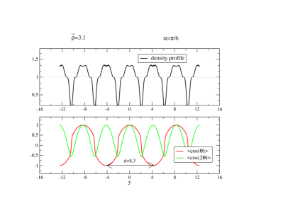
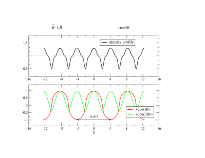
Figure 8: Density profile $P(y)$ and order parameters (calculated with respect to the $y-axis$ of laboratory frame) for the $S_{SB}$ phase obtained for ${{\overline{\rho}}=3.1}$ for cis molecules characterized by the angle $\alpha=\pi/6$ (Fig.2). Nematic order parameter $2\langle(\mathbf{b}\cdot\mathbf{\hat{y}})^{2}\rangle-1$ measured in the LAB is given by green colour and polar order parameter $\langle\mathbf{a}\cdot\mathbf{\hat{x}}\rangle$ by red colour. Alternating positive and negative parts of the polar order and the pitch of polar modulation is twice the period of density modulation, and of about 3 times molecule’s length is indicative of the splay bend formation.

These averages show the modulation of the density along with periodicity in the orientational degrees of freedom. The first of the two averages corresponds to the component of the nematic order parameter measured in the LAB, while the order parameter $\langle\mathbf{a}\cdot\mathbf{\hat{x}}\rangle$ is the average molecular polarization measured with respect to the x-axis of the LAB. The structure thus obtained is modulated and consists of layers, which makes it recognized as a smectic with a layer spacing (as seen in the density modulation) of approximately $d=4.15$. The pitch (approximately three molecular lengths) of the orientational modulation is twice the length of the density modulation, which, taking into account the behavior of the polar order parameter (red curve), is typical for splay bend deformations. The values of the nematic order parameter ($\left<cos2\theta\right>$) approach unity within the density layers and reach the value of $-0.5$ at the edges of the density layer. The profile of the polar order parameter ($\left<cos\theta\right>$) consists of identically shaped parts that alternate between positive and negative values. Within the layers, the density profile contains parts where the density is at a constant level, but the range of them is small. Slight fluctuations in the density curve are a numerical artifact. This we know since if a smaller number of Gaussian points is used, then they are getting much larger. At the same time, the orientational order parameters are not so sensitive to the accuracy of numerical integration.

In Fig.9, we present the density dependence of the director tilt angle (defined as the average orientation of the central molecular segment) for the phase $S_{SB}$, further supporting the hypothesis that the smectic phase is of the splay-bend type. Within the smectic layer it exhibits a practically linear dependence with distance, which is in agreement with the Monte Carlo simulations in Fig. 7. This result is of special importance because it is also the main assumption used to estimate the nematic-smectic splay bend boundaries for the full spectrum of conformers in the next subsection.

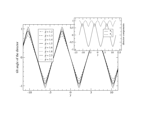
Figure 9: Reduced density dependence of tilt angle of the director with respect to the layer normal (parallel to the y-axis of laboratory system of frame) as calculated from the DFT theory for the $S_{SB}$ phase. Inset shows exemplary components of the director for $\overline{\rho}=1.5$.

In Fig. 10 we present the corresponding nematic order parameter profiles $<2(\mathbf{\hat{n}}(y)\cdot\mathbf{b})^{2}-1>$ calculated in the director frame for different densities.

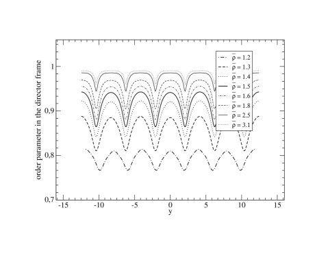
Figure 10: Nematic order parameter profiles $2\langle(\mathbf{\hat{n}}(y)\cdot\mathbf{b})^{2}\rangle-1$ in the director frame for the $S_{SB}$ phase for different densities.

These profiles have been obtained from the 2D local alignment tensor $\mathbf{Q}(y)$, whose components in the laboratory frame are given by

$$Q_{ij}=<2b_{i}b_{j}-\delta_{ij}>=n_{i}n_{j}<2(\mathbf{\hat{n}}\cdot\mathbf{b})^{2}-1>+m_{i}m_{j}<2(\mathbf{\hat{m}}\cdot\mathbf{b})^{2}-1>.$$ (13)

Here $\mathbf{\hat{n}}$ and $\mathbf{\hat{m}}$ of the components $n_{i}$, $m_{i}$, respectively, are local orthonormal eigenvectors of $\mathbf{Q}$ where the positive eigenvalue is associated with the director $\mathbf{\hat{n}}$. Unlike the $\mathbf{\hat{n}}\equiv-\mathbf{\hat{n}}$ symmetry of the director, $\mathbf{\hat{m}}$ is the polar vector, reflecting the polar nature of $S_{SB}$. As can be seen in Fig. 10 not only are the eigenvectors of $\mathbf{Q}$ positionally dependent, but the nematic order parameter profile $<2(\mathbf{\hat{n}}\cdot\mathbf{b})^{2}-1>$ exhibits weak modulation that decreases the more ordered phase for larger densities. However, the local orientational order of $S_{SB}$ is quite high. In Fig. 11 the local length $0\leq|<\mathbf{a}\cdot\mathbf{\hat{m}}>|\leq 1$ of the average polarization vector (which stays parallel to $\mathbf{\hat{m}}$) is presented for various reduced densities. Again, we observe a high, slightly modulated behavior of this observable in $S_{SB}$ of periodicity consistent with that of the nematic order parameter.

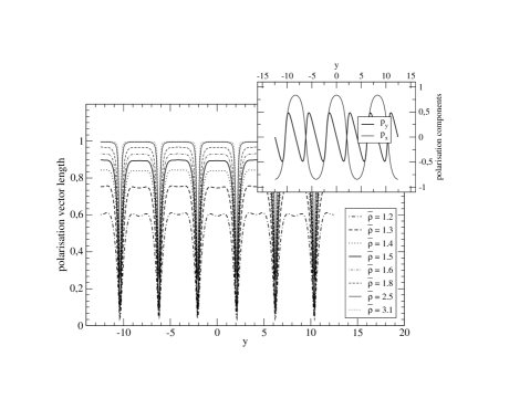
Figure 11: Length of the polarisation vector $|\langle\mathbf{\hat{m}}(y)\cdot\mathbf{a}\rangle|$ for different densities. Inset shows exemplary components of the polarization vector for $\overline{\rho}=1.4$. Please remind that average polarization is always perpendicular to the director for $S_{SB}$.

However, the periodicity of the average polarization vector, alternating with discontinuity between the positive and negative x-component, is twice that of the director (see inset in Fig.(11)). Furthermore, the transition temperature $N-S_{SB}$ for pure cis molecules is lower than in the simulations. A major cause of that is the neglect of the zigzag conformers. The value of the pitch $d=8.3$ is nearly constant for a wide range of densities. Only for the cases close to the $N-S_{SB}$ transition, which takes place at a density of about $\bar{\rho}=1.05$, it becomes slightly lower. For example, for $\bar{\rho}=1.2$ the pitch value is $d=7.9$.

The DFT splay-bend solutions for the system studied always exhibit a spatial modulation and are thus recognized as $S_{SB}$. However, with the ansatz $P(y)=const$ imposed on (7) it is still possible to obtain a stationary solution of Eq. (7) which is the pure nematic splay bend. Effectively, this can be achieved by using the following ansatz in the iteration process:

$$P(y,\theta)=\frac{P(y,\theta)}{\int P(y,\theta)d\theta},$$ (14)

along with the minimization of (8) with respect to period $d$. As a result, one can directly compare the free energies per particle of $N_{SB}$ and $S_{SB}$. This is shown in Fig. 12 where the free energy of $S_{SB}$ is found to be systematically lower than that of $N_{SB}$. With a decrease in the reduced density, the departure of the free energy of $S_{SB}$ from that of $N_{SB}$ becomes smaller and almost disappears near the $N-S_{SB}$ phase transition. However, no transition $N_{SB}-S_{SB}$ has been detected.

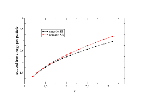
Figure 12: Reduced free energy per particle versus average density $\overline{\rho}$ for smectic- and nematic splay bend phases as obtained from DFT for cis molecules with arms titled at angle $\pi/6$.

IV.2 Bifurcations from isotropic and nematic phases

Our last step will be to use the full DFT formalism (7) for our model particles (Fig. 2) and to find the ordered phases that can bifurcate from the isotropic phase in the $(\alpha,\rho)$ plane. We will also estimate the phase boundaries in this plane between the nematic and smectic splay-bend assuming that the nematic phase is perfectly aligned.

The bifurcation scheme applied to equations such as (9) has been discussed in detail in a series of publications Kayser and Raveché (1978); Mulder (1989); Longa (1986a, b, 1989); Longa et al. (2005). Here, we generalize these results to the case with conformational degrees of freedom. We assume that the reference state is characterized by the distribution function $P_{0}(X)$. Then, at the bifurcation from state $P_{0}(X)$ to a new state $P(X)$ the difference $P(X)-P_{0}(X)$ is arbitrarily small, allowing one to linearize Eq.(9) about $P_{0}$. Simulations show that in the isotropic phase, all conformers are equally populated, allowing us to take $P_{0}(X)=P_{0}(s)\equiv P_{I}=const$. Similarly, we assume that $P_{0}(X)$ is known for ideally oriented molecules in the nematic phase. If we are only interested in finding the densities of bifurcations, it is sufficient to analyze the linearized form of Eq. (9) given by

$$P(X)=Z_{0}^{-1}\left(1-\overline{\rho}S\underset{(X_{2})}{{Tr}}\left\{\Theta\left[\xi(X,X_{2})-r_{12}\right]\,P(X_{2})\right\}\right),$$ (15)

with $Z_{0}$ calculated for $P_{0}$. For the analysis of liquid crystalline phases (with the exception of $S_{SB}$), we decompose the probability distribution function $P(X)$ into a complete and orthonormal basis $F_{\alpha}$

$$P(y,\theta,\mathbf{s})=\sum_{\alpha}\langle F_{\alpha}\rangle F_{\alpha}(y,\theta,\mathbf{s}),$$ (16)

where $F_{\alpha}(y,\theta,\mathbf{s})$ is the product of orthonormal functions in separate subspaces. It reads:

$$F_{\alpha}(y,\theta,\mathbf{s})\equiv F_{abkl\sigma}(y,\theta,\mathbf{s})=n_{abkl\sigma}\psi_{a}(ky)\phi_{b}(l\theta)f_{\sigma}(\mathbf{s}),$$ (17)

where $n_{abkl\sigma}$ is the normalization constant and where discrete indices $\{a,b,k,l,\sigma\}$ are sequentially numbered with a single index $\alpha$, where low $\{k,l,\sigma\}$s correspond to low values of $\alpha$. The spatial y-dependent functions $\psi_{a}(ky)$ are discrete Fourier cos and sin modes

$$\psi_{a}(ky)=\left\{\begin{matrix}\cos(\frac{2\pi ky}{d}),&a=1\\ \sin(\frac{2\pi ky}{d}),&a=2,\end{matrix}\right.$$ (18)

where $k=0,1,2,...$, and where $d$ is the periodicity of the structure ($S=L^{2},\,L=Md,\,M\in\mathbb{N}$). Angle-dependent functions $\phi_{b}(l\theta)$ are

$$\phi_{b}(l\theta)=\left\{\begin{matrix}\cos(l\theta),&b=1\\ \sin(l\theta),&b=2,\end{matrix}\right.$$ (19)

where $l=0,1,2,...$. Finally, the four purely conformational functions $f_{\sigma}(\mathbf{s})\equiv f_{\sigma}(s_{1},s_{2})$ are given by

$$f_{\sigma}(s_{1},s_{2})=\left\{\begin{matrix}\frac{1}{2},&\sigma=0\\ \frac{s_{1}+s_{2}}{2\sqrt{2}},&\sigma=1\\ \frac{s_{1}-s_{2}}{2\sqrt{2}},&\sigma=2\\ \frac{1}{2}s_{1}s_{2},&\sigma=3\,.\end{matrix}\right.$$ (20)

The normalization constant $n_{abkl\sigma}$ is such that

$$Tr_{(X)}\left[F_{abkl\sigma}\left(y,\theta,\mathbf{s}\right)F_{a^{\prime}b^{\prime}k^{\prime}l^{\prime}\sigma^{\prime}}\left(y,\theta,\mathbf{s}\right)\right]=\delta_{aa^{\prime}}\delta_{bb^{\prime}}\delta_{kk^{\prime}}\delta_{ll^{\prime}}\delta_{\sigma\sigma^{\prime}},$$ (21)

which allows identification: $\langle F_{\alpha}\rangle=Tr_{(X)}\left[P(y,\theta,\mathbf{s})F_{\alpha}\left(y,\theta,\mathbf{s}\right)\right]$. Substituting (17) into (21) explicitly gives

$$n^{2}_{abkl\sigma}=\frac{2}{\pi L}\left[1-\left(\frac{1}{2}\right)^{2-a}\delta_{k0}\right]\left[1-\left(\frac{1}{2}\right)^{2-b}\delta_{l0}\right].$$ (22)

The first term $\langle F_{\alpha=0}\rangle=F_{\alpha=0}(y,\theta,\mathbf{s})\equiv\langle F_{11000}\rangle=F_{11000}(y,\theta,\mathbf{s})$ in the expansion (16) is the normalization constant of $P(X)$. The remaining terms $\langle F_{\alpha\neq 0}\rangle$ are the order parameters. For example, $\langle F_{1102\sigma}\rangle$ are the leading order parameters of nematics. Nonzero $k$s indicate in the smectic ordering, which can be non-polar (only even $l$s are present) or polar (at least $l=1$ is present).

The index $\sigma$ classifies the order parameters according to the local($k\neq 0$)/global($k=0$) population of various conformational states. More specifically, for a structure of $\sigma=0$, each conformer population is represented with equal probability. The order parameters with $\sigma=1$ measure the polar order, and they vanish for chiral conformers. In contrast to case $\sigma=1$, the order parameters with $\sigma=2$ are responsible for the chiral order, since there are only chiral conformers that contribute to this. Finally, the order parameters with $\sigma=3$ measure the relative local/global importance of chiral and non-chiral conformers for a given phase. If we are interested in the (local) concentration of a given fraction of conformers, these are found by performing a simple average over $P(X)$. For example, the concentration of the fraction zigzag+ is given by

$$\langle\delta_{s_{1},1}\delta_{s_{2},-1}\rangle=\frac{F_{abkl0}}{4}+\frac{\langle F_{abkl2}\rangle}{\sqrt{2}}-\frac{\langle F_{abkl3}\rangle}{2},$$ (23)

where $\delta_{i,j}$ is the Kronecker delta.

Using the definitions introduced above, we can now proceed with the identification of states that bifurcate from the reference one. In the first step, we expand the kernel $Z_{0}^{-1}S\Theta\left[\xi(X^{{}^{\prime}}_{1},X^{{}^{\prime}}_{2})-r^{{}^{\prime}}_{12}\right]$ in the basis $F_{\alpha}(X)$, substitute the expansion for the equation (15), multiply both sides by $F_{\gamma}(X)$ and trace over $X$. This procedure reduces Eq. (15) to a set of linear equations for $\langle F_{\gamma}\rangle$

$$\langle F_{\gamma}\rangle=\langle F_{0}\rangle\delta_{\gamma 0}-\overline{\rho}\sum_{\beta}\Theta_{\gamma\beta}\langle F_{\beta}\rangle,$$ (24)

where

$$\Theta_{\alpha\beta}=Z_{0}^{-1}S\underset{(X^{{}^{\prime}}_{1}X^{{}^{\prime}}_{2})}{{Tr}}\left\{F_{\alpha}(X^{{}^{\prime}}_{1})\Theta\left[\xi(X^{{}^{\prime}}_{1},X^{{}^{\prime}}_{2})-r^{{}^{\prime}}_{12}\right]F_{\beta}(X^{{}^{\prime}}_{2})\right\},$$ (25)

and where the above calculations are limited to the $n\times n$ matrix $\Theta_{\alpha\beta}$, corresponding to the leading terms in (17), usually of $k\leq 2$ and $l\leq 2$, which generally makes the linear equation (24) of order $n\leq 100$.

The next step is diagonalization of the matrix $\Theta_{\alpha\beta}$. Let $\Theta_{\alpha\beta}$=$p_{\alpha\mu}\lambda^{\theta}_{\mu}(\mathbf{p}^{-1})_{\mu\beta}$ where $\lambda^{\theta}_{\mu}$ are eigenvalues of $\Theta_{\alpha\beta}$ and $\mathbf{p}$ transforms $\Theta_{\alpha\beta}$ into diagonal form. With the aid of $\mathbf{p}$, equation (24) can be rewritten in a simpler form. It reads:

$$\langle\chi_{\alpha}\rangle=(\mathbf{p}^{-1})_{\alpha 0}\langle F_{0}\rangle-\overline{\rho}\lambda^{\theta}_{\alpha}\langle\chi_{\alpha}\rangle,$$ (26)

where $\chi_{\alpha}=\sum_{\beta}(\mathbf{p}^{-1})_{\alpha\beta}F_{\beta}$. Now, candidates $\{\chi_{\mu}\}$ for the bifurcating states are those that do not couple with $\langle F_{0}\rangle$ i.e for which $(\mathbf{p}^{-1})_{\mu 0}\langle F_{0}\rangle=0$. The second condition is that the corresponding $\{\lambda^{\theta}_{\mu}\}$ are real negative numbers. With these restrictions, we are left with a set of homogeneous equations $\,\{\langle\chi_{\mu}\rangle=-\overline{\rho}\lambda^{\theta}_{\mu}\langle\chi_{\mu}\rangle\,\}$ for $\langle\chi_{\mu}\rangle\$, which produce non-zero solutions for $\langle\chi_{\mu}\rangle$ given that $\overline{\rho}\geq\overline{\rho}^{*}_{\mu}$, where $\overline{\rho}^{*}_{\mu}=-\frac{1}{\lambda^{\theta}_{\mu}}$. The first bifurcating state $\overline{\rho}^{*}_{\mu_{0}}$ corresponds to the minimal density among $\{\overline{\rho}^{*}_{\mu}\}$: $\overline{\rho}^{*}_{\mu_{0}}=\mathrm{Min}\{\overline{\rho}^{*}_{\mu}\}$. The corresponding bifurcating probability density distribution function is given by $P(X)=P_{0}(X)+\epsilon\chi_{\mu_{0}}(X)$, where arbitrarily small $\epsilon\equiv\langle\chi_{\mu_{0}}\rangle$, can be determined with the higher order perturbation calculations.

IV.2.1 Bifurcations from isotropic phase

We found the bifurcation densities from the isotropic phase to the different nematic and smectic phases using a full set of degrees of freedom. In our analysis $k=1$, $a=1$ or $2$ (Eq. 18), $l$ ranges from $0$ to $2$ for $b$ equal to $1$ or $2$ (Eq. 19), and $\sigma$ varies from $0$ to $3$ (Eq. 20). This limits the size of the matrix $\Theta_{\alpha\beta}$ for the bifurcation analysis to $40$ by $40$. Due to the dependence of $\Theta_{\alpha\beta}$ on the wave vector, for any specific opening angle $\alpha$ of particles, Fig. (2), we diagonalize a series of matrices, each for a different wave vector, and find the eigenvalue that gives the lowest bifurcating density. For diagonalization, we used the Jacobi method involving Givens rotations, since these matrices were all symmetrical. The results are presented in Fig. 6, where the dark gray line corresponds to the bifurcation from the isotropic phase ($I$) to (chiral) nematic ($N$) phase, green line from the isotropic phase to the so-called mixed phase (M) and the blue line from isotropic to chiral smectic A ($S_{A}^{*}$). The corresponding bifurcation probability densities $P(y,\theta,\boldsymbol{s})$ are:

(a) for the $I-N$ bifurcation (dark gray line):

$$\begin{split}P(y,\theta,\boldsymbol{s})\approx&\frac{1}{8\pi S}+\varepsilon[\alpha_{0}\cos(2\theta)f_{0}(s_{1},s_{2})\\ &+\alpha_{1}\sin(2\theta)f_{2}(s_{1},s_{2})+\alpha_{2}\cos(2\theta)f_{3}(s_{1},s_{2})+...\,].\end{split}$$ (27)

The coefficients $\{\alpha_{i},i=0,1,2\}$ are presented in Fig. 13 in dark gray, similar to that of the phase diagram in Fig. 6. The leading term $\alpha_{0}\cos(2\theta)f_{0}(s_{1},s_{2})$ represents the nematic order with an equal fraction of different conformers. The next term $\alpha_{1}\sin(2\theta)f_{2}(s_{1},s_{2})$ becomes relevant for $\alpha>0$. It monitors the appearance and increase of chiral fractions (zigzags) with increasing $\alpha$, with a maximum fraction achieved when the central molecular segment is oriented at $\theta=\pm\pi/4$ with respect to the director. This means that the overall nematic phase becomes macroscopically chiral. At the same time, the concentration of cis-type particles along the director outweighs the concentration of the chiral conformers ($\alpha_{2}>0$), in agreement with Monte Carlo simulations, Fig. 4;

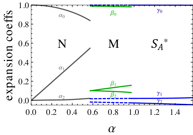
Figure 13: Coefficients of decomposition of bifurcating states in the $F_{\gamma}$-basis for $N$, $M$ and $S_{A}^{*}$ structures.

(b) for the $I-M$ bifurcation (green line: $0.18\pi\lesssim\alpha\lesssim 0.31\pi$), where $M$ stands for the ’mixed phase’, the situation is more complex because the two different smectic phases of nearly equal bifurcation densities compete (green line, dashed blue line). The phase of slightly lower density is given by the probability density:

$$\begin{split}P(y,\theta,\boldsymbol{s})\approx&\frac{1}{8\pi S}+\varepsilon[\beta_{0}\sin\left(\frac{2\pi y}{d}\right)f_{0}(s_{1},s_{2})+\beta_{1}\cos\left(\frac{2\pi y}{d}\right)\sin(\theta)f_{1}(s_{1},s_{2})\\ &+\beta_{2}\sin\left(\frac{2\pi y}{d}\right)\cos(2\theta)f_{0}(s_{1},s_{2})+...].\end{split}$$ (28)

The structure is of the smectic type ($\beta_{0}>0$). It has a period of approximately $d\approx 10.1$ for all opening angles $\alpha$ of the particles and is characterized by the coefficients $\beta$ as shown in Fig. 13. Given the period of the structure (roughly three molecular lengths) and the polarization wave of the cis-conformers ($\beta_{1}\neq 0$) it can be identified as a non-chiral smectic splay-bend ordering;

(c) for the $I-S_{A}^{*}$ bifurcation (blue line):

$$\begin{split}P(y,\theta,\boldsymbol{s})\approx&\frac{1}{8\pi S}+\varepsilon[\gamma_{0}\cos\left(\frac{2\pi y}{d}\right)f_{0}(s_{1},s_{2})+\gamma_{1}\cos\left(\frac{2\pi y}{d}\right)\sin(2\theta)f_{2}(s_{1},s_{2})\\ &+\gamma_{2}\sin\left(\frac{2\pi y}{d}\right)\sin(\theta)f_{1}(s_{1},s_{2})+...].\end{split}$$ (29)

The period of this structure is practically constant and equal to $d=4.25$ for all opening angles of the particles. The coefficients $\{\gamma_{i},i=0,1,2\}$ are shown in Fig. 13 as continuous blue lines. Here, the dominant $\gamma_{0}$-term is of a smectic A type. Furthermore, the presence of the chiral term, proportional to $\gamma_{1}$, makes zigzag molecules preferred in this phase. These results remain in agreement with the simulations and allow us to identify this phase as chiral smectic A ($S_{A}^{*}$). They also explain why it is so difficult to unequivocally interpret the $M$ structure in Monte Carlo simulations. The reason is that the dashed blue line representing bifurcation to $S_{A}^{*}$ in the phase diagram, Fig. 6, nearly overlaps the green line that describes the competing smectic structure (28).

IV.2.2 Bifurcations from ideally ordered nematic phase

Monte Carlo simulations and the results of previous sections revealed that at the transition from nematic to smectic splay bend the particles are highly ordered about the director. Therefore, to study a bifurcation from an ordinary nematic phase to more ordered phases, we can assume the perfect nematic order approximation Karbowniczek et al. (2017), where the central molecular segments always stay parallel to the director ($\mathbf{\hat{n}}(y)\cdot\mathbf{b_{i}}=1,\,i=1...N$). Now, we can proceed as before by expanding $P(y,s)$ in the basis $F_{abk0\sigma}(y,\theta,\mathbf{s})$, where in the ideal nematic order approximation the terms $\phi_{b}(l\theta)$ are dropped. As a consequence, the problem is reduced to the diagonalization of 20 by 20 matrices for the period $d$, which minimizes the density of the bifurcation. Results are shown as a red line in the phase diagram.

V Conclusions

Since the seminal work of Onsager on steric interactions in nematics Onsager (1949), simulations and theoretical works that invoke the packing entropy provided important insights into the self-assembly of densely packed systems, especially liquid crystals. Without escaping from the main idea that molecular shape is the primary factor in the formation of different liquid crystalline structures, our attempt here was to add a new factor, namely conformational degrees of freedom. We used simple three-segment calamitic particles under strong planar confinement to probe the structural behavior of the LC samples. We assumed four predominant conformations per molecule cis$\pm$ and trans$\pm$ ones. Therefore, the model served as the simplest example in which an interplay between packing entropy and sterically restricted conformational entropy can be studied in detail. So far only separate systems, composed of cis$+$ or trans$+$ rigid trimers were considered.

We were particularly interested in the formation of splay-bend and chiral ordering previously reported for cis$+$ and trans$+$, respectively. Using constant pressure Monte Carlo simulations and Onsager-type density functional theory, we showed that the presence of conformational degrees of freedom leads to a rich spectrum of stable phases where different average fractions of conformers combine to determine properties of the resulting phases. While in the isotropic phase all fractions are equally populated and the phase is nonchiral, the ordered phases that are formed from the isotropic phase are all macroscopically chiral. The chirality of ordered phases is a function of density and opening angle, and the study of the average fraction of the trans- and cis- conformers revealed that the nematic and splay-bend phases are dominated by the achiral cis conformers, while the chiral zigzags prevail in the $S_{A}^{*}$ phase. Hence we observe conformationally and sterically induced isotropic-nematic- and isotropic-smectic chiral symmetry breaking (CSB). In both, the nematic and smectic $A^{*}$ phases domains of opposite chiralities are formed as a manifestation of CSB.

We obtain a bifurcation from the isotropic to the nematic phase and two bifurcations from the isotropic to the smectic phases without an intermediate nematic phase. We also find that in both smectic phases, the period $d$ of the smectic structures at bifurcation does not depend on the opening angle and is equal to $10.1$ in $M$ and $4.25$ in the $S_{A}^{*}$ phases. Surprisingly good qualitative agreement of these results with the constant-pressure Monte Carlo simulations is obtained along with structure identification. Furthermore, difficulties in stabilizing the $M$ phase in MC simulations are explained by the proximity of a competing $S_{A}^{*}$ phase, as seen in the bifurcation analysis of the corresponding Onsager model.

The most interesting observation is an identification of the smectic splay-bend phase. Although $S_{SB}$ is dominated by the $cis\pm$ conformers, the $zigzag\pm$ ones are also present, occupying with maximal probability the places where the steric polarization wave changes sign. They seem to help in stabilizing the smectic ordering. As stated in the Introduction, the concurrent, long-sought splay-bend nematic phase has been detected recently in colloidal systems of bent-core particles. However, a novel grand potential Landau-deGennes theory as well as simulations suggest that the alleged splay-bend phase stabilizing in colloidal systems to display density modulations. Our flexible trimers are also forming stable $S_{SB}$. Therefore, it seems that the stable splay-bend phase appears to have the key symmetry of smectics. However, the bifurcation analysis does not exclude the pure nematic splay-bend solutions.

The structures obtained in the simulations do not have a true long-range order; however, the nematic of the particles with a small angle $\alpha$ and smectics seems to form domains with the largest correlation length. We showed that despite the plethora of functions used in the literature, $g_{2}(r)$ is a sufficiently good indicator of (quasi-) liquid crystal phase transitions for the particles studied. We also provided a detailed theoretical description of the results obtained in the simulations.

Finally, the subject of molecules with conformational degrees of freedom has been addressed by Tavarone et. al.Tavarone, Charbonneau, and Stark (2016) in their kinetic Monte Carlo modeling of conformational changes taking place when photo-switchable molecules of the derivative of the dye Methyl-Red are attached to a surface and subjected to linearly polarized light. In the cited work, the generated photo-induced change in molecular shape was represented by straight and bent needles.

Our model, which takes into account equilibrium trans—-cis, but ignores the monomer fraction and assumes that open and cyclic acid trimers are formed instantaneously and with equal probability, can also be viewed as a simplified description of the hydrogen bond dissociation-association process. We think that at least some of the steady states trans—-cis of the complexes should be qualitatively similar to the equilibrium configurations predicted by this work. As such studies have not been explored in monolayer liquid crystal science, it would be interesting to see how more complex scenarios, e.g. with monomers and energetic factors describing complex formation influence the resulting entropy-induced orientational order.

References

- Meyer (1976) R. B. Meyer, Proceedings of the Les Houches Summer School on Theoretical Physics, 1973, session No. XXV (New York: Gordon and Breach, 1976).
- Cestari et al. (2011) M. Cestari, S. Diez-Berart, D. A. Dunmur, A. Ferrarini, M. R. de La Fuente, D. J. B. Jackson, D. O. López, G. R. Luckhurst, M. A. Perez-Jubindo, R. M. Richardson, J. Salud, B. A. Timimi, and H. Zimmermann, Phys. Rev. E 84, 031704 (2011).
- Chen et al. (2013a) D. Chen, J. H. Porada, J. B. Hooper, et al., Proc. Natl. Acad. Sci. USA 110, 15931 (2013a).
- Borshch et al. (2013a) V. Borshch, Y.-K. Kim, J. Xiang, et al., Nat. Commun. 4, 1 (2013a).
- Mandle (2016) R. J. Mandle, Soft Matter 12, 7883 (2016).
- Tavarone, Charbonneau, and Stark (2015) R. Tavarone, P. Charbonneau, and H. Stark, The Journal of Chemical Physics 143, 114505 (2015), https://doi.org/10.1063/1.4930886 .
- Karbowniczek et al. (2017) P. Karbowniczek, M. Ciesla, L. Longa, and A. Chrzanowska, Liquid Crystals 44, 254 (2017), https://doi.org/10.1080/02678292.2016.1259510 .
- Karbowniczek (2018) P. Karbowniczek, The Journal of Chemical Physics 148, 136101 (2018), https://doi.org/10.1063/1.5021541 .
- Dozov (2001) I. Dozov, Europhys. Lett. 56, 247 (2001).
- de Gennes and Prost (1993) P. G. de Gennes and J. Prost, The Physics of Liquid Crystals, 2nd ed. (Clarendon Press, 1993).
- Jákli, Lavrentovich, and Selinger (2018) A. Jákli, O. D. Lavrentovich, and J. V. Selinger, Rev. Mod. Phys. 90, 045004 (2018).
- Longa and Trebin (1990) L. Longa and H.-R. Trebin, Phys. Rev. A 42, 3453 (1990).
- Longa and Paja̧k (2016) L. Longa and G. Paja̧k, Phys. Rev. E 93, 040701 (2016).
- Paja̧k, Longa, and Chrzanowska (2018) G. Paja̧k, L. Longa, and A. Chrzanowska, Proceedings of the National Academy of Sciences 115, E10303 (2018), https://www.pnas.org/doi/pdf/10.1073/pnas.1721786115 .
- Šepelj et al. (2007) M. Šepelj, A. Lesac, U. Baumeister, S. Diele, H. L. Nguyen, and D. W. Bruce, J. Mater. Chem. 17, 1154 (2007).
- Panov et al. (2010) V. P. Panov, M. Nagaraj, J. K. Vij, Y. P. Panarin, A. Kohlmeier, M. G. Tamba, R. A. Lewis, and G. H. Mehl, Phys. Rev. Lett. 105, 167801 (2010).
- Borshch et al. (2013b) V. Borshch, Y.-K. Kim, J. Xiang, M. Gao, A. Jákli, V. P. Panov, J. K. Vij, C. T. Imrie, M. G. Tamba, G. H. Mehl, and O. D. Lavrentovich, Nat. Commun. 4, 2635 (2013b).
- Chen et al. (2013b) D. Chen, J. H. Porada, J. B. Hooper, A. Klittnick, Y. Shen, M. R. Tuchband, E. Korblova, D. Bedrov, D. M. Walba, M. A. Glaser, J. E. Maclennan, and N. A. Clark, Proc. Natl. Acad. Sci. USA 110, 15931 (2013b).
- Paterson et al. (2016) D. A. Paterson, M. Gao, Y.-K. Kim, A. Jamali, K. L. Finley, B. Robles-Hernández, S. Diez-Berart, J. Salud, M. R. de La Fuente, B. A. Timimi, H. Zimmermann, C. Greco, A. Ferrarini, J. M. D. Storey, D. O. López, O. D. Lavrentovich, G. R. Luckhurst, and C. T. Imrie, Soft Matter 12, 6827 (2016).
- López et al. (2016) D. O. López, B. Robles-Hernández, J. Salud, M. R. de La Fuente, N. Sebastian, S. Diez-Berart, X. Jaen, D. A. Dunmur, and G. R. Luckhurst, Phys. Chem. Chem. Phys. 18, 4394 (2016).
- Görtz et al. (2009) V. Görtz, C. Southern, N. W. Roberts, H. F. Gleeson, and J. W. Goodby, Soft Matter 5, 463 (2009).
- Chen et al. (2014) D. Chen, M. Nakata, R. Shao, M. R. Tuchband, M. Shuai, U. Baumeister, W. Weissflog, D. M. Walba, M. A. Glaser, J. E. Maclennan, and N. A. Clark, Phys. Rev. E 89, 022506 (2014).
- Wang et al. (2015) Y. Wang, G. Singh, D. M. Agra-Kooijman, M. Gao, H. K. Bisoyi, C. Xue, M. R. Fisch, S. Kumar, and Q. Li, CrystEngComm 17, 2778 (2015).
- Al-Janabi, Mandle, and Goodby (2017) A. Al-Janabi, R. J. Mandle, and J. Goodby, RSC Adv. 7, 47235 (2017).
- Mandle and Goodby (2016) R. J. Mandle and J. W. Goodby, ChemPhysChem 17, 967 (2016).
- Jansze et al. (2015) S. M. Jansze, A. Martinez-Felipe, J. M. D. Storey, A. T. M. Marcelis, and C. T. Imrie, Angewandte Chemie - International Edition 54, 643 (2015).
- Fernández-Rico et al. (2020) C. Fernández-Rico, M. Chiappini, T. Yanagishima, H. de Sousa, D. G. A. L. Aarts, M. Dijkstra, and R. P. A. Dullens, Science 369, 950 (2020), https://www.science.org/doi/pdf/10.1126/science.abb4536 .
- Merkel et al. (2018) K. Merkel, A. Kocot, J. K. Vij, and G. Shanker, Phys. Rev. E 98, 022704 (2018).
- Meyer et al. (2020) C. Meyer, C. Blanc, G. R. Luckhurst, P. Davidson, and I. Dozov, Science Advances 6, eabb8212 (2020), https://www.science.org/doi/pdf/10.1126/sciadv.abb8212 .
- Meyer, Luckhurst, and Dozov (2015) C. Meyer, G. R. Luckhurst, and I. Dozov, J. Mater. Chem. C 3, 318 (2015).
- Yun et al. (2015) C.-J. Yun, M. R. Vengatesan, J. K. Vij, and J.-K. Song, Applied Physics Letters 106, 173102 (2015), https://doi.org/10.1063/1.4919065 .
- Babakhanova et al. (2017) G. Babakhanova, Z. Parsouzi, S. Paladugu, H. Wang, Y. A. Nastishin, S. V. Shiyanovskii, S. Sprunt, and O. D. Lavrentovich, Phys. Rev. E 96, 062704 (2017).
- Archbold et al. (2017) C. T. Archbold, R. J. Mandle, J. L. Andrews, S. J. Cowling, and J. W. Goodby, Liquid Crystals 00, 1 (2017).
- Józefowicz and Longa (2007) W. Józefowicz and L. Longa, Molecular Crystals and Liquid Crystals 478, 115/[871] (2007), https://doi.org/10.1080/15421400701738586 .
- Vaupotič et al. (2014) N. Vaupotič, M. Čepič, M. A. Osipov, and E. Gorecka, Physical Review E - Statistical, Nonlinear, and Soft Matter Physics 89, 2 (2014).
- Lubensky and Radzihovsky (2002) T. C. Lubensky and L. Radzihovsky, Phys. Rev. E 66, 031704 (2002).
- Goodby (2017) J. W. Goodby, Liquid Crystals 44, 1755 (2017), https://doi.org/10.1080/02678292.2017.1347293 .
- Delaire and Nakatani (2000) J. A. Delaire and K. Nakatani, Chemical Reviews 100, 1817 (2000), pMID: 11777422, https://doi.org/10.1021/cr980078m .
- Katsonis et al. (2007) N. Katsonis, M. Lubomska, M. M. Pollard, B. L. Feringa, and P. Rudolf, Progress in Surface Science 82, 407 (2007).
- Browne and Feringa (2009) W. R. Browne and B. L. Feringa, Annual Review of Physical Chemistry 60, 407 (2009), pMID: 18999995, https://doi.org/10.1146/annurev.physchem.040808.090423 .
- Fang et al. (2010) G. Fang, Y. Shi, J. E. Maclennan, N. A. Clark, M. J. Farrow, and D. M. Walba, Langmuir 26, 17482 (2010), pMID: 20929215, https://doi.org/10.1021/la102788j .
- Wu et al. (2021) Y. Wu, Y. Liu, J. Chen, and R. Yang, Crystals 11 (2021), 10.3390/cryst11121560.
- Peón et al. (2006) J. Peón, J. Saucedo-Zugazagoitia, F. Pucheta-Mendez, R. A. Perusquía, G. Sutmann, and J. Quintana-H, The Journal of Chemical Physics 125, 104908 (2006), https://doi.org/10.1063/1.2338313 .
- Varga et al. (2009) S. Varga, P. Gurin, J. C. Armas-Pérez, and J. Quintana-H, The Journal of Chemical Physics 131, 184901 (2009), https://doi.org/10.1063/1.3258858 .
- J. Martínez-González (2012) J. Q.-H. J. Martínez-González, J. C. Armas-Pérez, J. Stat. Phys. 150, 559 (2012).
- Józefowicz and Longa (2011) W. Józefowicz and L. Longa, Molecular Crystals and Liquid Crystals 545, 204/[1428] (2011), https://doi.org/10.1080/15421406.2011.572014 .
- Cinacchi et al. (2017) G. Cinacchi, A. Ferrarini, A. Giacometti, and H. B. Kolli, The Journal of Chemical Physics 147, 224903 (2017), https://doi.org/10.1063/1.4996610 .
- Schlotthauer et al. (2015) S. Schlotthauer, R. A. Skutnik, T. Stieger, and M. Schoen, The Journal of Chemical Physics 142, 194704 (2015), https://doi.org/10.1063/1.4920979 .
- Anzivino, van Roij, and Dijkstra (2020) C. Anzivino, R. van Roij, and M. Dijkstra, The Journal of Chemical Physics 152, 224502 (2020), https://doi.org/10.1063/5.0008936 .
- Anzivino, van Roij, and Dijkstra (2022) C. Anzivino, R. van Roij, and M. Dijkstra, Phys. Rev. E 105, L022701 (2022).
- Chrzanowska (2016) A. Chrzanowska, Ferroelectrics 495, 43 (2016), https://doi.org/10.1080/00150193.2016.1136730 .
- Chrzanowska (2017) A. Chrzanowska, Phys. Rev. E 95, 063316 (2017).
- Kayser and Raveché (1978) R. F. Kayser and H. J. Raveché, Phys. Rev. A 17, 2067 (1978).
- Mulder (1989) B. Mulder, Phys. Rev. A 39, 360 (1989).
- Longa (1986a) L. Longa, The Journal of Chemical Physics 85, 2974 (1986a), https://doi.org/10.1063/1.451007 .
- Longa (1986b) L. Longa, Zeitschrift für Physik B Condensed Matter 64, 357 (1986b).
- Longa (1989) L. Longa, Liquid Crystals 5, 443 (1989), https://doi.org/10.1080/02678298908045395 .
- Longa et al. (2005) L. Longa, P. Grzybowski, S. Romano, and E. Virga, Phys. Rev. E 71, 051714 (2005).
- Onsager (1949) L. Onsager, Annals of the New York Academy of Sciences 51, 627 (1949).
- Tavarone, Charbonneau, and Stark (2016) R. Tavarone, P. Charbonneau, and H. Stark, The Journal of Chemical Physics 144, 104703 (2016), https://doi.org/10.1063/1.4943393 .