Eigenvalue estimates for the magnetic Hodge Laplacian on differential forms

Abstract

In this paper we introduce the magnetic Hodge Laplacian, which is a generalization of the magnetic Laplacian on functions to differential forms. We consider various spectral results, which are known for the magnetic Laplacian on functions or for the Hodge Laplacian on differential forms, and discuss similarities and differences of this new “magnetic-type” operator.

1 Introduction and statement of results

The classical magnetic Laplacian on a Riemannian manifold $(M^{n},g)$ associated to a smooth real $1$-form $\alpha\in\Omega^{1}(M)$ acts on the space of smooth complex-valued functions $C^{\infty}(M,\mathbb{C})$ and is given by

$$\Delta^{\alpha}=\delta^{\alpha}d^{\alpha},$$ (1.1)

where $d^{\alpha}:=d^{M}+i\alpha$ and $\delta^{\alpha}:=\delta^{M}-i\langle\alpha^{\sharp},\cdot\rangle$ (note that $\delta^{M}$ is the $L^{2}$-adjoint of $d^{M}$). Here $\alpha^{\sharp}\in{\mathcal{X}}(M)$ is the vector field corresponding to the $1$-form $\alpha$ via the musical isomorphism $\langle\alpha^{\sharp},X\rangle=\alpha(X)$. The $1$-form $\alpha$ is called the magnetic potential and $d^{M}\alpha$ is the magnetic field. The magnetic Laplacian $\Delta^{\alpha}$ can be viewed as a first order perturbation of the usual Laplacian $\Delta^{M}=\delta^{M}d^{M}$, namely for any $f\in C^{\infty}(M,\mathbb{C})$,

$$\Delta^{\alpha}f=\Delta^{M}f-2i\langle\operatorname{grad}f,\alpha^{\sharp}\rangle+(|\alpha^{\sharp}|^{2}-i\,{\rm{div}}\,\alpha^{\sharp})f.$$ (1.2)

In the case of a closed manifold or a compact manifold with boundary, both operators $\Delta^{M}$ and $\Delta^{\alpha}$ (with suitable boundary conditions when $\partial M\neq\emptyset$) have a discrete spectrum with ascending eigenvalues with multiplicity denoted by $(\lambda_{k}(M))_{k\in\mathbb{N}}$ and $(\lambda_{k}^{\alpha}(M))_{k\in\mathbb{N}}$, respectively. There are very few Riemannian manifolds where the complete set of eigenvalues can be given explicitly. Amongst them are the unit round sphere $\mathbb{S}^{n}$ with the standard metric $g$, whose eigenfunctions can be described as spherical harmonics. In Appendix A, we give an explicit derivation of the spectrum of a magnetic Laplacian on $(\mathbb{S}^{3},g)$ with a special magnetic potential $\alpha$. This derivation is based on the Hopf fibration $\mathbb{S}^{1}\hookrightarrow\mathbb{S}^{3}\rightarrow\mathbb{S}^{2}$, and $\alpha$ is a constant magnetic field along the $\mathbb{S}^{1}$-fibers.

In analogy with the generalization of the usual Laplacian $\Delta^{M}$ on functions to the Hodge Laplacian $\delta^{M}d^{M}+d^{M}\delta^{M}$ on differential forms, it is natural to generalize the magnetic Laplacian on functions to complex differential forms as follows. On the set of complex-valued differential forms $\Omega(M,\mathbb{C})$, we define

$$\Delta^{\alpha}:=\delta^{\alpha}d^{\alpha}+d^{\alpha}\delta^{\alpha}$$

where $d^{\alpha}:=d^{M}+i\alpha\wedge$ and $\delta^{\alpha}:=\delta^{M}-i\alpha^{\sharp}\lrcorner$ is its formal adjoint. Both $d^{\alpha}$ and $\delta^{\alpha}$ can also be expressed via the magnetic covariant derivative $\nabla^{\alpha}_{X}Y:=\nabla^{M}_{X}Y+i\alpha(X)Y$ for any $X,Y\in C^{\infty}(TM\otimes\mathbb{C})$ (see formula (3.1)). We refer to this operator $\Delta^{\alpha}$ acting on $\Omega^{p}(M,\mathbb{C})$ as the magnetic Hodge Laplacian on complex $p$-forms.

We establish the following results for the magnetic Hodge Laplacian on an oriented Riemannian manifold $(M^{n},g)$:

• We show that the magnetic Hodge Laplacian commutes with the Hodge star operator (see Corollary 3.2).

• We derive a magnetic analogue of the classical Bochner-Weitzenböck formula (see Theorem 3.4).

• We prove gauge invariance of the magnetic Laplacian on forms $\Delta^{\alpha}$ (see Corollary 3.8).

• Following a result by Gallot-Meyer [13] for the Hodge Laplacian, we derive a lower bound for the first eigenvalue of the magnetic Hodge Laplacian for closed manifolds (see Theorem 4.2).

• Following a result by Colbois-El Soufi-Ilias-Savo [6] for the magnetic Laplacian on functions, we derive an upper bound for the first eigenvalue of the magnetic Hodge Laplacian for closed manifolds (see Theorem 4.3).

• We show that the diamagnetic inequality does not hold for magnetic Hodge Laplacians (Corollary 4.5). In fact, we give a counterexample which is based on the calculations in Appendix A.

• Following Raulot-Savo in [25], we derive a Reilly formula for the magnetic Hodge Laplacian on Riemannian manifolds with boundary (see Theorem 5.1) and use it to derive a lower bound for the first eigenvalue of the magnetic Hodge Laplacian on an embedded hypersurface of a Riemannian manifold (see Theorem 6.2).

• Following Guérini-Savo in [14], we derive a “gap” estimate between the first eigenvalues of consecutive $p$-values of the magnetic Hodge Laplacians on $\Omega^{p}(M,\mathbb{C})$ for isometrically immersed manifolds $(M^{n},g)$ in Euclidean space $\mathbb{R}^{n+m}$ (see Theorem 6.3).

Acknowledgment: The third named author thanks University of Durham for its hospitality during his stay. He also thanks the Alexander von Humboldt foundation and the Alfried Krupp Wissenschaftskolleg in Greifswald.

2 Review of the magnetic Laplacian for functions

Before we introduce the magnetic Hodge Laplacian in the next section, we first recall some results for the classical magnetic Laplacian on functions. Let $(M^{n},g)$ be a Riemannian manifold and $\alpha\in\Omega^{1}(M)$. The magnetic Laplacian $\Delta^{\alpha}$ acting on complex-valued smooth functions defined by formula (1.1) has the property of gauge invariance, that is $\Delta^{\alpha}(e^{-if})=e^{-if}\Delta^{\alpha-d^{M}f}$ for any smooth real-valued function $f$. When $M$ is compact (with or without boundary), the spectrum of $\Delta^{\alpha}$ (or with suitable boundary conditions when $\partial M\neq\emptyset$) is discrete. Therefore, by the gauge invariance, the spectrum of $\Delta^{\alpha}$ is equal to the spectrum of $\Delta^{\alpha-d^{M}f}$. Thus, when $\alpha$ is exact, the spectrum of $\Delta^{\alpha}$ reduces to that of the usual Laplace-Beltrami operator. In [8, Prop. 3], it is proven that one can always assume that $\alpha$ is a co-closed $1$-form (and tangential, i.e. $\nu\lrcorner\alpha=0$, when $M$ has a boundary) without changing the spectrum of $\Delta^{\alpha}$. Moreover, by using the Hodge decomposition on compact manifolds, the authors show in [6, Prop. 1] that one can further consider $\alpha$ to be of the form

$$\alpha=\delta^{M}\psi+h,$$

where $\psi$ is a $2$-form on $M$ (with $\nu\lrcorner\psi=0$ when $\partial M\neq\emptyset$), and $h$ is a harmonic $1$-form on $M$, that is, $d^{M}h=\delta^{M}h=0$ (with $\nu\lrcorner h=0$ when $\partial M\neq\emptyset$), and again the spectrum does not change. Here, we point out that the first eigenvalue $\lambda^{\alpha}_{1}(M)$ of $\Delta^{\alpha}$ is not necessarily zero like for the usual Laplacian $\Delta^{M}$ as shown in [28, Ex. 1]. This interesting property of the magnetic Laplacian was characterized by Shigekawa (see [28, Prop. 3.1 and Thm. 4.2]) as follows.

Theorem 2.1 (Shigekawa).

Let $(M^{n},g)$ be a closed Riemannian manifold and

$$\mathfrak{B}_{M}=\left\{\alpha_{\tau}:=\frac{d^{M}\tau}{i\tau}:\tau\in C^{\infty}(M,\mathbb{S}^{1})\right\}.$$

Then the following are equivalent:

• $\alpha\in\mathfrak{B}_{M}$,

• $d^{M}\alpha=0$ and $\int_{C}\alpha\in 2\pi\mathbb{Z}$ for all closed curves $C$ in $M$,

• $\lambda_{1}^{\alpha}(M)=0$.

Hence, when $\alpha$ cannot be gauged away, meaning that $\alpha$ does not belong to the set $\mathfrak{B}_{M}$, the first eigenvalue is necessarily positive. This gauge invariance can be described by the following: If $\alpha_{\tau}\in\mathfrak{B}_{M}$ for some $\tau\in C^{\infty}(M,\mathbb{S}^{1})$, the Laplacians $\Delta^{\alpha}$ and $\Delta^{\alpha+\alpha_{\tau}}$ are unitarily equivalent, that is

$$\bar{\tau}\Delta^{\alpha}\tau=\Delta^{\alpha+\alpha_{\tau}}.$$

Thus $\Delta^{\alpha}$ and $\Delta^{\alpha+\alpha_{\tau}}$ have the same spectrum as stated before. Now, the diamagnetic inequality compares the first eigenvalue of $\Delta^{\alpha}$ to the one for the Laplacian $\Delta^{M}$ and says that

$$\lambda_{1}^{\alpha}(M)\geq\lambda_{1}(M),$$

with equality if and only if the magnetic potential $\alpha$ can be gauged away. When $M$ has no boundary, the diamagnetic inequality provides no information since $\lambda_{1}(M)=0$. However, when we consider manifolds with boundary and the magnetic Laplacian is associated to the Dirichlet or Robin boundary conditions, the diamagnetic inequality still holds and tells us, in particular, that the first eigenvalue $\lambda_{1}^{\alpha}(M)$ is always positive.

A simple estimate for the first eigenvalue of the magnetic Laplacian can be deduced straightforwardly from the min-max principle. Indeed, when applying the Rayleigh quotient to a constant function, we get, after choosing $\delta^{M}\alpha=0$, i.e. $\operatorname{div}\alpha^{\sharp}=0$, that

$$\lambda^{\alpha}_{1}(M)\leq\frac{\int_{M}|\alpha|^{2}d\mu_{g}}{{\rm Vol}(M)}\leq||\alpha||^{2}_{\infty}.$$

Several papers have been devoted to estimating the first eigenvalue of the magnetic Laplacian, see, for example,[2, 5, 12, 16, 17, 20, 8, 9, 10, 7, 11, 6]. Among these results, we quote two of them [11], [6] on closed Riemannian manifolds.

The first result gives the magnetic Lichnerowicz-type estimates for the first two eigenvalues:

Theorem 2.2 (see [11, Thm 1.1]).

Let $(M^{n},g)$ be a closed Riemannian manifold of dimension $n\geq 2$ and $\alpha\in\Omega^{1}(M)$. If

$$\mathrm{Ric}^{M}\geq C>0\qquad\text{and}\qquad\lVert d^{M}\alpha\rVert_{\infty}\leq\left(1+2\sqrt{\frac{n-1}{n}}\right)^{-1}C,$$ (2.1)

then we have

$$0\leq\lambda^{\alpha}_{1}(M)\leq a_{-}(C,\lVert d^{M}\alpha\rVert_{\infty},n)\qquad\text{ and }\qquad\lambda^{\alpha}_{2}(M)\geq a_{+}(C,\lVert d^{M}\alpha\rVert_{\infty},n),$$ (2.2)

where

$$a_{\pm}(C,A,n)=n\cdot\frac{(C-A)\pm\sqrt{(C-A)^{2}-4(\frac{n-1}{n})A^{2}}}{2(n-1)}.$$

The technique used to obtain this result is an integral Bochner-type formula which involves the magnetic Hessian that is associated to the magnetic covariant derivative $\nabla^{\alpha}$. A related result to Theorem 2.2 for the magnetic Laplacian with Robin boundary conditions on compact Riemannian manifolds $(M,g)$ with smooth boundary was proved in [15]. In the setup of the above theorem, it is natural to ask whether the estimates are sharp for some $\alpha$ that is not gauged away. For this, we will test the example of the round sphere $\mathbb{S}^{3}$ where the magnetic field $\alpha$ is collinear to the Killing vector field that defines the Hopf fibration. We refer to Appendix A for more details on the computation.

Example (Unit sphere $\mathbb{S}^{3}$ with $\alpha=tY_{2}$).

Let $(\mathbb{S}^{3},g)$ be the unit sphere in $\mathbb{R}^{4}$ with standard metric $g$ of curvature $1$. We use the notation introduced in Appendix A. Let $\alpha=tY_{2}$ where $Y_{2}$ is the unit Killing vector field on $\mathbb{S}^{3}$. Using (A.6), we obtain $d^{M}\alpha=2t\,Y_{3}\wedge Y_{4}$ where $\{Y_{2},Y_{3},Y_{4}\}$ is an orthonormal frame of $T\mathbb{S}^{3}$ and, therefore, $\|d^{M}\alpha\|_{\infty}=2t$. Since $\mathrm{Ric}^{M}=C=2$, condition (2.1) is satisfied for $|t|\leq\frac{\sqrt{3}}{\sqrt{3}+\sqrt{8}}=t_{\rm{max}}\approx 0.38$, and for $t\in[0,t_{\rm{max}}]$ we have, by (2.2),

$$\lambda_{1}^{\alpha}(\mathbb{S}^{3})\leq\frac{3}{2}\left[(1-t)-\sqrt{(1-t)^{2}-\frac{8}{3}t^{2}}\right]\\ \leq\frac{3}{2}\left[(1-t)+\sqrt{(1-t)^{2}-\frac{8}{3}t^{2}}\right]\leq\lambda_{2}^{\alpha}(\mathbb{S}^{3}).$$

On the other hand, we conclude from (A.9) that $\lambda_{1}^{\alpha}(\mathbb{S}^{3})=t^{2}$ and $\lambda_{2}^{\alpha}(\mathbb{S}^{3})=3-2t+t^{2}$ for small $t\in[0,t_{\rm{max}}]$. The relations between these two smallest eigenvalues and their estimates for small $t>0$ are illustrated in Figure 1.

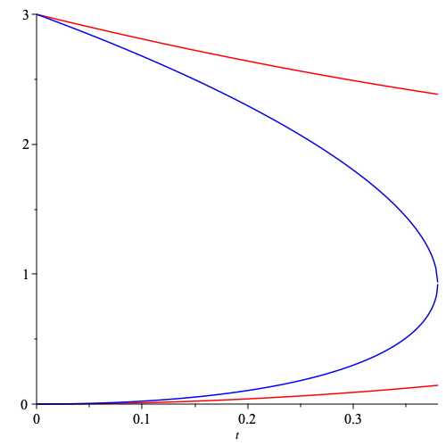
Figure 1: Eigenvalues $\lambda_{1}^{\alpha}(\mathbb{S}^{3})$ and $\lambda_{2}^{\alpha}(\mathbb{S}^{3})$ in red and upper and lower bounds in blue, as functions over $t\in[0,t_{\rm{max}}]$.

As we can see from Figure 1, sharpness of the upper estimate of $\lambda_{1}^{\alpha}(\mathbb{S}^{3})$ is lost (see the discussion after Lemma 4.1).

The second result was given in [6] in the general setting of magnetic Schrödinger operators $\Delta^{\alpha}+q$ with Neumann boundary conditions. For simplicity, we formulate it in the special case of a closed Riemannian manifold $(M^{n},g)$ with vanishing potential $q=0$. We will return to this estimate later in Subsection 4.2.

Theorem 2.3 ([6, Thm. 2]).

Let $(M^{n},g)$ be a closed Riemannian manifold and let $\alpha\in\Omega^{1}(M)$ be of the form $\alpha=\delta^{M}\psi+h$ with $\psi\in\Omega^{2}(M)$ and $h$ a harmonic $1$-form. Then,

$$\lambda_{1}^{\alpha}(M)\leq\frac{1}{{\rm{vol}}(M)}\left(d(h,\mathcal{L}_{\mathbb{Z}})^{2}+\frac{\|d^{M}\alpha\|^{2}}{\lambda_{1,1}^{\prime\prime}(M)}\right),$$

where $\lambda_{1,1}^{\prime\prime}(M)$ is the first eigenvalue of the Hodge Laplacian $\Delta^{M}$ on co-exact $1$-forms, $\mathcal{L}_{\mathbb{Z}}$ is the lattice of integer harmonic $1$-forms in $\Omega^{1}(M)$, and

$$d(h,\mathcal{L}_{\mathbb{Z}})=\inf_{\eta\in\mathcal{L}_{\mathbb{Z}}}\|h-\eta\|^{2}.$$

In order to check the sharpness of this inequality, we consider again the case of the round sphere with the magnetic field given by the Killing vector field.

Example (Unit sphere $\mathbb{S}^{3}$ with $\alpha=tY_{2}$).

Let $(\mathbb{S}^{3},g)$ be the unit round sphere in $\mathbb{R}^{4}$ with standard metric $g$ of curvature $1$ and let $\alpha=tY_{2}$. Since $H^{1}(\mathbb{S}^{3})=0$ and $\delta^{M}\alpha=0$, $\alpha$ is co-exact and therefore of the form $\delta^{M}\psi$ for some $\psi\in\Omega^{2}(M)$. Moreover, we have from [13, p. 37], [22] that $\lambda_{1,1}^{\prime\prime}(\mathbb{S}^{3})=4$. Thus, Theorem 2.3 yields

$$\lambda_{1}^{\alpha}(\mathbb{S}^{3})\leq\frac{1}{4\rm{vol}(\mathbb{S}^{3})}\int_{\mathbb{S}^{3}}|d^{M}\alpha|^{2}d\mu_{g}=t^{2},$$

that is, the upper estimate of the first magnetic eigenvalue is sharp for this case.

Finally, as we mention in the introduction, examples of closed Riemannian manifolds $(M^{n},g)$ with non-trivial magnetic potential $\alpha\in\Omega^{1}(M)$ (that is, magnetic potential which cannot be gauged away), for which the full spectrum of the magnetic Laplacian $\Delta^{\alpha}$ can be explicitly given, are very scarce (see, for example, [8, 7] for such computations).

3 The magnetic Hodge Laplacian for differential forms

In this section, we introduce the magnetic Hodge Laplacian for differential forms, prove a magnetic Bochner formula, and discuss its gauge invariance. Henceforth $(M^{n},g)$ will denote an oriented $n$-dimensional Riemannian manifold and $\Omega^{p}(M)$ and $\Omega^{p}(M,\mathbb{C})$ will denote the spaces of real and complex differential $p$-forms for $0\leq p\leq n$. The spaces of real and complex vector fields on $M$ are denoted by ${\mathcal{X}}(M)$ and ${\mathcal{X}}_{\mathbb{C}}(M)$. To simplify notation, we will often identify real and complex vector fields with real and complex 1-forms via the (complex-linear) musical isomorphisms. That is, $\Omega^{1}(M,\mathbb{C})\to{\mathcal{X}}_{\mathbb{C}}(M);\,\omega\mapsto\omega^{\sharp}$ given by $\omega(X)=\langle X,\overline{\omega^{\sharp}}\rangle$, where $\langle\cdot,\cdot\rangle$ stands for the Hermitian scalar product extended from the Riemannian metric $g$ to ${\mathcal{X}}_{\mathbb{C}}(M)$.

3.1 The magnetic Hodge Laplacian

Fix a smooth $1$-form $\alpha\in\Omega^{1}(M)$ (a magnetic potential) and consider the magnetic differential on $\Omega^{p}(M,\mathbb{C})$, given by

$$d^{\alpha}:=d^{M}+i\alpha\wedge.$$

It is not difficult to check that the $L^{2}$-adjoint of $d^{\alpha}$ acting on complex differential forms (when $M$ is without boundary) w.r.t. the Hermitian inner product

$$\int_{M}\langle\omega,\eta\rangle\,d\mu_{g}=\int_{M}*(\omega\wedge*\bar{\eta})\,d\mu_{g}$$

is given by

$$\delta^{\alpha}:=\delta^{M}-i\alpha^{\sharp}\lrcorner,$$

where $\delta^{M}=(-1)^{n(p+1)+1}*d^{M}*$ is the formal adjoint of $d^{M}$ on $p$-forms (both extended complex linearly to complex differential forms) and the Hodge star operator is extended to a complex linear operator $*:\Omega^{p}(M,\mathbb{C})\to\Omega^{n-p}(M,\mathbb{C})$. Recall here that the interior product “$\lrcorner$” is the pointwise adjoint of the wedge product “$\wedge$”. Both $d^{\alpha}$ and $\delta^{\alpha}$ are the differential and co-differential associated to the magnetic connection on differential forms $\nabla^{\alpha}_{X}:=\nabla^{M}_{X}+i\alpha(X)$ on $\Omega^{p}(M,\mathbb{C})$. That means we have

$$d^{\alpha}=\sum_{j=1}^{n}e_{j}^{*}\wedge\nabla^{\alpha}_{e_{j}}\quad\text{and}\quad\delta^{\alpha}=-\sum_{j=1}^{n}e_{j}\lrcorner\nabla^{\alpha}_{e_{j}},$$ (3.1)

where $\{e_{1},\cdots,e_{n}\}$ is a local orthonormal frame of $TM$. Now, we define the magnetic Hodge Laplacian acting on $\Omega^{p}(M,\mathbb{C})$ as follows:

$$\Delta^{\alpha}:=d^{\alpha}\delta^{\alpha}+\delta^{\alpha}d^{\alpha}.$$

We first have the following observation:

Lemma 3.1.

On differential $p$-forms, we have $*d^{\alpha}=(-1)^{p+1}\delta^{\alpha}*$ and $*\delta^{\alpha}=(-1)^{p}d^{\alpha}*$.

Proof.

The proof is straightforward from the fact that $*d^{M}=(-1)^{p+1}\delta^{M}*$ and $*(\alpha\wedge)=(-1)^{p}\alpha^{\sharp}\lrcorner*$ on $p$-forms. Also, we have that $*\delta^{M}=(-1)^{p}d^{M}*$ and $*(\alpha^{\sharp}\lrcorner)=(-1)^{p+1}\alpha\wedge*$. ∎

The following is an immediate consequence of Lemma 3.1 above.

Corollary 3.2.

The magnetic Hodge Laplacian $\Delta^{\alpha}$ commutes with the Hodge star operator.

Proof.

Indeed, on $p$-forms, we have

$$\Delta^{\alpha}* = (d^{\alpha}\delta^{\alpha}+\delta^{\alpha}d^{\alpha})*$$

$$= (-1)^{p+1}d^{\alpha}*d^{\alpha}+(-1)^{p}\delta^{\alpha}*\delta^{\alpha}$$

$$= *(\delta^{\alpha}d^{\alpha}+d^{\alpha}\delta^{\alpha})=*\Delta^{\alpha}.$$

∎

The magnetic Laplacian $\Delta^{\alpha}$ has the same principal symbol as the Hodge Laplacian $\Delta^{M}$ (see Equation (3.10) in the next section), since it differs by lower order terms. Therefore, it is an elliptic, essentially self-adjoint operator acting on smooth complex forms on a closed oriented Riemannian manifold or acting on smooth complex forms with Dirichlet boundary condition on an oriented Riemannian manifold with boundary (see Subsection 5.1 below). Therefore, $\Delta^{\alpha}$ has a discrete spectrum consisting of nonnegative eigenvalues $(\lambda_{j,p}^{\alpha}(M))_{j\in\mathbb{N}}$, denoted in ascending order with multiplicities. Moreover, as for the usual Hodge Laplacian, its spectrum on $p$-forms is the same as the one on $(n-p)$-forms and the first eigenvalue is characterized by

$$\lambda_{1,p}^{\alpha}(M)={\rm inf}\left\{\frac{\int_{M}(|d^{\alpha}\omega|^{2}+|\delta^{\alpha}\omega|^{2})d\mu_{g}}{\int_{M}|\omega|^{2}d\mu_{g}}\right\},$$ (3.2)

where $\omega$ runs over all smooth $p$-forms with $\omega|_{\partial M}=0$, if $\partial M\neq\emptyset$.

We also note that the differential $d^{\alpha}$ does not satisfy the crucial property $d^{\alpha}\circ d^{\alpha}=0$ to introduce cohomology groups. In fact, we have

$$(d^{\alpha})^{2}=id^{M}\alpha\wedge$$ (3.3)

with $d^{M}\alpha\in\Omega^{2}(M)$ is the magnetic field. We could, however, still define magnetic Betti numbers and a magnetic Euler characteristic via

$$b_{j}^{\alpha}(M)=\dim{\rm Ker}(\Delta^{\alpha}|_{\Omega^{j}(M,\mathbb{C})})$$

and

$$\chi^{\alpha}(M)=\sum_{j=0}^{n}(-1)^{j}b_{j}^{\alpha}(M).$$

Corollary 3.2 implies that $b_{j}^{\alpha}(M)=b_{n-j}^{\alpha}(M)$, and that the magnetic Euler characteristic vanishes in the case of odd dimension $n$. Moreover, we have $b_{0}^{\alpha}(M)=b_{n}^{\alpha}(M)=0$ for any magnetic potential $\alpha$ that cannot be gauged away, that is $\alpha\notin\mathfrak{B}_{M}$. It may be interesting to investigate these magnetic Betti numbers with regards to their information about the Riemannian manifold $(M,g)$.

3.2 A magnetic Bochner formula

Recall that the Hodge Laplacian $\Delta^{M}:=d^{M}\delta^{M}+\delta^{M}d^{M}$ is related to the Bochner Laplacian on $M$ via a curvature term by the Bochner-Weitzenböck formula. Namely, we have (see, e.g, [23, Thm. 7.4.5] or [30, p. 14])

$$\Delta^{M}=\nabla^{*}\nabla+\mathcal{B}^{[p]},$$ (3.4)

where $\mathcal{B}^{[p]}$, called the Bochner operator, is a symmetric endomorphism on $\Omega^{p}(M)$ given by $\mathcal{B}^{[p]}=\sum_{j,k=1}^{n}e_{k}^{*}\wedge(e_{j}\lrcorner R^{M}(e_{j},e_{k}))$. Here $R^{M}$ is the curvature operator acting on differential forms associated to the Levi-Civita connection $\nabla^{M}$ which is given by $R^{M}(X,Y)=[\nabla^{M}_{X},\nabla^{M}_{Y}]-\nabla^{M}_{[X,Y]}$ for all $X,Y\in{\mathcal{X}}(M)$ and $\{e_{1},\ldots,e_{n}\}$ is a local orthonormal frame of $TM$. The Bochner Laplacian $\nabla^{*}\nabla$ is given by

$$\nabla^{*}\nabla=-\sum_{j=1}^{n}\nabla^{M}_{e_{j}}\nabla_{e_{j}}^{M}+\sum_{j=1}^{n}\nabla^{M}_{\nabla^{M}_{e_{j}}e_{j}}.$$

In the following, we derive a similar magnetic Bochner-Weitzenböck formula for $\Delta^{\alpha}$, which will provide a relation between the Hodge Laplacians $\Delta^{\alpha}$ and $\Delta^{M}$. For this, we recall the following definition. Given an Euclidean vector space $V$ and an endomorphism $A:V\to V$, there exists a canonical extension $A^{[p]}$ of $A$ on the set of alternating $p$-forms ($p\geq 1$) given by $A^{[p]}:\Lambda^{p}(V^{*})\to\Lambda^{p}(V^{*})$ via

$$(A^{[p]}\omega)(v_{1},\dots,v_{p})=\sum_{j=1}^{p}\omega(v_{1},\dots,Av_{j},\dots,v_{p}),$$ (3.5)

for $v_{1},\cdots,v_{p}\in V$. By convention, we take $A^{[0]}=0$. One can easily show from the definition that the endomorphism $A^{[p]}$ can be written in terms of $A$ as

$$A^{[p]}=\sum_{j=1}^{n}e_{j}^{*}\wedge(A(e_{j})\lrcorner),$$ (3.6)

where $\{e_{1},\ldots,e_{n}\}$ is an orthonormal frame of $V$. If $A$ is a symmetric (resp. skew-symmetric) endomorphism on $V$, then so is $A^{[p]}$ on $\Lambda^{p}(V^{*})$. In this case, if we denote the eigenvalues of $A$ by $\eta_{1}\leq\cdots\leq\eta_{n}$, then we have the following estimates. For any $\omega\in\Lambda^{p}(V^{*})$

$$\langle A^{[p]}\omega,\omega\rangle\geq\sigma_{p}|\omega|^{2}\quad\text{and}\quad\langle A^{[p]}\omega,\omega\rangle\leq(\sigma_{n}-\sigma_{n-p})|\omega|^{2}\leq p\|A\|\cdot|\omega|^{2},$$ (3.7)

where $\sigma_{p}:=\eta_{1}+\cdots+\eta_{p}$ are called the $p$-eigenvalues of $A^{[p]}$ and $\|A\|$ is the operator norm of $A$. In order to state the magnetic Bochner-Weitzenböck formula, we introduce the following magnetic Bochner operator on $\Omega^{p}(M,\mathbb{C})$:

$$\mathcal{B}^{[p],\alpha}:=\sum_{j,k=1}^{n}e_{k}^{*}\wedge\left(e_{j}\lrcorner R^{\alpha}(e_{j},e_{k})\right),$$

where as before $\{e_{i}\}_{i=1,\ldots,n}$ is a local orthonormal frame of $TM$. Here $R^{\alpha}$ is the curvature operator associated to the magnetic covariant derivative $\nabla^{\alpha}$, that is

$$R^{\alpha}(X,Y)Z=\nabla^{\alpha}_{X}\nabla^{\alpha}_{Y}Z-\nabla^{\alpha}_{Y}\nabla^{\alpha}_{X}Z-\nabla^{\alpha}_{[X,Y]}Z$$

for $X,Y,Z\in{\mathcal{X}}_{\mathbb{C}}(M)$. Now, we express the magnetic Bochner operator in terms of the classical one by the following

Lemma 3.3.

On the set of complex differential $p$-forms, the magnetic Bochner operator $\mathcal{B}^{[p],\alpha}$ satisfies

$$\mathcal{B}^{[p],\alpha}=\mathcal{B}^{[p]}-iA^{[p],\alpha},$$

where $A^{[p],\alpha}$ is the canonical extension to complex $p$-forms of the skew-symmetric endomorphism $A^{\alpha}$ on $TM$ given by $A^{\alpha}(X)=(X\lrcorner d^{M}\alpha)^{\sharp}$ for any vector field $X$ on $M$.

Proof.

An easy computation shows that, for any $X,Y\in{\mathcal{X}}(M)$ and $\omega\in\Omega^{p}(M,\mathbb{C}),$

$$R^{\alpha}(X,Y)\omega=R^{M}(X,Y)\omega+i(d^{M}\alpha)(X,Y)\omega.$$

The proof can then be deduced from the definition of $\mathcal{B}^{[p],\alpha}$ and the fact that $A^{\alpha}$ is skew-symmetric. ∎

We make the following observation. Using the identity $*(X^{\flat}\wedge)=(-1)^{p}X\lrcorner*$ valid for any vector field $X$, one can easily show that $\mathcal{B}^{[p]}=(-1)^{p(n-p)}*\mathcal{B}^{[n-p]}*$ which gives that $\langle\mathcal{B}^{[p]}\cdot,\cdot\rangle=\langle\mathcal{B}^{[n-p]}*\cdot,*\cdot\rangle$ where $*$ is the Hodge star operator on $M$ and $\langle\cdot,\cdot\rangle$ is the pointwise Hermitian product on $\Omega^{p}(M,\mathbb{C})$. In the same way, and since the endomorphism $A^{\alpha}$ is skew-symmetric, one can also show that $A^{[p],\alpha}=(-1)^{p(n-p)}*A^{[n-p],\alpha}*$. Therefore, we deduce that $\mathcal{B}^{[p],\alpha}=(-1)^{p(n-p)}*\mathcal{B}^{[n-p],\alpha}*$ and, thus,

$$\langle\mathcal{B}^{[p],\alpha}\cdot,\cdot\rangle=\langle\mathcal{B}^{[n-p],\alpha}*\cdot,*\cdot\rangle$$ (3.8)

on complex $p$-forms. Notice here that $iA^{[p],\alpha}$ is a symmetric endomorphism on $\Omega^{p}(M,\mathbb{C})$. We now formulate the magnetic Bochner-Weitzenböck formula.

Theorem 3.4 (Magnetic Bochner-Weitzenböck formula).

Let $(M^{n},g)$ be a Riemannian manifold and $\alpha\in\Omega^{1}(M)$. Then we have

$$\Delta^{\alpha}=(\nabla^{\alpha})^{*}\nabla^{\alpha}+\mathcal{B}^{[p],\alpha},$$ (3.9)

where $(\nabla^{\alpha})^{*}\nabla^{\alpha}=-\sum_{j=1}^{n}\nabla^{\alpha}_{e_{j}}\nabla^{\alpha}_{e_{j}}+\sum_{j=1}^{n}\nabla^{\alpha}_{\nabla_{e_{j}}^{M}e_{j}}$. Moreover, we have

$$\Delta^{\alpha}=\Delta^{M}-iA^{[p],\alpha}+i(\delta^{M}\alpha)-2i\nabla^{M}_{\alpha}+|\alpha|^{2}.$$ (3.10)

Proof.

The proof follows the same computations as for the Hodge Laplacian $\Delta^{M}$. For this, we use the expressions of $d^{\alpha}$ and $\delta^{\alpha}$ in (3.1) on an orthonormal frame $\{e_{j}\}_{j=1}^{n}$ on $TM$ chosen in a way that $\nabla^{M}e_{j}=0$ at some point $x\in M$. By the fact that, for all $X,Y\in{\mathcal{X}}_{\mathbb{C}}(M)$, we have $\nabla^{\alpha}_{X}(Y\wedge\cdot)=(\nabla^{M}_{X}Y)\wedge\cdot+Y\wedge\nabla^{\alpha}_{X}\cdot$, which can be proven by a straighforward computation (the same relation holds for the interior product), we can write at $x\in M$:

$$\Delta^{\alpha} = d^{\alpha}\delta^{\alpha}+\delta^{\alpha}d^{\alpha}$$

$$= -\sum_{j,k=1}^{n}e_{k}^{*}\wedge\nabla^{\alpha}_{e_{k}}(e_{j}\lrcorner\nabla^{\alpha}_{e_{j}})-\sum_{j,k=1}^{n}e_{j}\lrcorner\nabla^{\alpha}_{e_{j}}(e_{k}^{*}\wedge\nabla^{\alpha}_{e_{k}})$$

$$= -\sum_{j,k=1}^{n}e_{k}^{*}\wedge(e_{j}\lrcorner\nabla^{\alpha}_{e_{k}}\nabla^{\alpha}_{e_{j}})-\sum_{j,k=1}^{n}e_{j}\lrcorner(e_{k}^{*}\wedge\nabla^{\alpha}_{e_{j}}\nabla^{\alpha}_{e_{k}})$$

$$= -\sum_{j,k=1}^{n}e_{k}^{*}\wedge(e_{j}\lrcorner\nabla^{\alpha}_{e_{k}}\nabla^{\alpha}_{e_{j}})-\sum_{j=1}^{n}\nabla^{\alpha}_{e_{j}}\nabla^{\alpha}_{e_{j}}+\sum_{j,k=1}^{n}e_{k}^{*}\wedge(e_{j}\lrcorner\nabla^{\alpha}_{e_{j}}\nabla^{\alpha}_{e_{k}})$$

$$= -\sum_{j=1}^{n}\nabla^{\alpha}_{e_{j}}\nabla^{\alpha}_{e_{j}}+\sum_{j,k=1}^{n}e_{k}^{*}\wedge(e_{j}\lrcorner R^{\alpha}(e_{j},e_{k})),$$

where in the fourth equality we used the relation

$$X\lrcorner(\beta\wedge\cdot)=(X\lrcorner\beta)\wedge\cdot+(-1)^{\deg\beta}\beta\wedge(X\lrcorner\cdot),$$

for any differential form $\beta$. This shows that (3.9) holds. To obtain (3.10), we just combine Lemma 3.3 with the Bochner-Weitzenböck formula (3.4) and the fact that at $x\in M$

$$(\nabla^{\alpha})^{*}\nabla^{\alpha} = -\sum_{j=1}^{n}\nabla^{\alpha}_{e_{j}}\nabla^{\alpha}_{e_{j}}$$

$$= -\sum_{j=1}^{n}\nabla^{M}_{e_{j}}(\nabla^{M}_{e_{j}}+i\alpha(e_{j}))-i\sum_{j=1}^{n}\alpha(e_{j})(\nabla^{M}_{e_{j}}+i\alpha(e_{j}))$$

$$= \nabla^{*}\nabla+i\delta^{M}\alpha-2i\nabla^{M}_{\alpha}+|\alpha|^{2}.$$

∎

Remark.

Formula (3.10) is a generalisation of the formula for the magnetic Laplacian for functions, given by

$$\Delta^{\alpha}f=\delta^{\alpha}d^{\alpha}f=\Delta^{M}f+i(\delta^{M}\alpha)f-2i\alpha(f)+|\alpha|^{2}f,$$

since $A^{[0],\alpha}=0$.

Now, we will consider a particular case for the magnetic field $\alpha$. We will assume that it is a Killing 1-form, that is its corresponding vector field $\alpha^{\sharp}$ by the musical isomorphism is a Killing vector field, and show that Equation (3.10) can be expressed in a more compact way. In addition, if the Killing 1-form $\alpha$ has constant norm, we will show that the exterior differential $d^{M}$ and codifferential $\delta^{M}$ both commute with the magnetic Laplacian. Notice here that, in general, $d^{\alpha}$ and $\delta^{\alpha}$ do not commute with $\Delta^{\alpha}$ as a consequence from (3.3), even when $\alpha^{\sharp}$ is just a Killing 1-form.

Proposition 3.5.

Let $(M^{n},g)$ be a Riemannian manifold and let $\alpha$ be a Killing $1$-form, then

$$\Delta^{\alpha}=\Delta^{M}-2i\mathcal{L}_{\alpha}+|\alpha|^{2},$$ (3.11)

where $\mathcal{L}_{\alpha}$ is the Lie derivative in the direction of $\alpha$. Moreover, if the norm of $\alpha$ is constant, we have that $\Delta^{\alpha}d^{M}=d^{M}\Delta^{\alpha}$ and $\Delta^{\alpha}\delta^{M}=\delta^{M}\Delta^{\alpha}$ and, therefore, the magnetic Laplacian preserves the set of exact and co-exact forms.

Proof.

The fact that $\alpha$ is Killing gives $A^{\alpha}(X)=X\lrcorner d^{M}\alpha=2\nabla^{M}_{X}\alpha$ for any vector field $X\in TM$. Therefore, we get by (3.6) that

$$A^{[p],\alpha}=\sum_{j=1}^{n}e_{j}^{*}\wedge(A^{\alpha}(e_{j})\lrcorner)=2\sum_{j=1}^{n}e_{j}^{*}\wedge(\nabla^{M}_{e_{j}}\alpha\lrcorner)=2T^{[p],\alpha},$$

where $T^{[p],X}$ is the canonical extension of the endomorphism $T^{X}=\nabla^{M}X$, for any $X$, given by the expression in (3.6). Now, the identity $\mathcal{L}_{X}=\nabla^{M}_{X}+T^{[p],X}$ valid on $p$-forms for any vector field $X$ on $TM$ [26, Lem. 2.1] allows us to deduce that

$$2\mathcal{L}_{\alpha}=2\nabla^{M}_{\alpha}+A^{[p],\alpha}.$$ (3.12)

Hence, Equation (3.10) gives the desired identity. Here, we also use that $\delta^{M}\alpha=0$ as a consequence from the fact that $\alpha$ is Killing. Since $d^{M}$ commutes with $\Delta^{M}$ and with $\mathcal{L}_{\alpha}$ as well as with $|\alpha|^{2}$ which is constant, we deduce that $d^{M}$ commutes with $\Delta^{\alpha}$. That the codifferential $\delta^{M}$ commutes with $\Delta^{\alpha}$ comes from the fact that $\delta^{M}$ commutes with $\Delta^{M}$ and with $\mathcal{L}_{\alpha},$ which is a consequence of $\delta^{M}=\pm*d^{M}*$ and $\mathcal{L}_{\alpha}*=*\mathcal{L}_{\alpha}$ by Equation (3.12). Recall here that $A^{[p],\alpha}*=*A^{[n-p],\alpha}$. This finishes the proof. ∎

When the magnetic potential $\alpha$ is Killing of constant norm on $(M^{n},g)$, we have seen that the magnetic Laplacian $\Delta^{\alpha}$ preserves the set of exact and co-exact forms on $M$. In the following, we will assume $M$ to be compact and will let $\lambda_{1,p}^{\alpha}(M)$ be the first positive eigenvalue of $\Delta^{\alpha}$ on differential $p$-forms and $\lambda_{1,p}^{\alpha}(M)^{\prime}$ (resp. $\lambda_{1,p}^{\alpha}(M)^{\prime\prime}$) be the first positive eigenvalue restricted to exact (resp. co-exact) $p$-forms. As in the standard case [25], we can prove by differentiating eigenforms that $\lambda_{1,p}^{\alpha}(M)^{\prime\prime}=\lambda_{1,p+1}^{\alpha}(M)^{\prime}$ and by Hodge duality that $\lambda_{1,p}^{\alpha}(M)^{\prime\prime}=\lambda_{1,n-p}^{\alpha}(M)^{\prime}$. Recall here that the magnetic Laplacian commutes with the Hodge star operator. However, we will see in the next proposition, that the relation $\lambda_{1,p}^{\alpha}(M)={\rm min}(\lambda_{1,p}^{\alpha}(M)^{\prime},\lambda_{1,p}^{\alpha}(M)^{\prime\prime})$ that usually holds for the Laplacian $\Delta^{M}$ is not always true for $\Delta^{\alpha}$.

For the next proposition, we need the following well known result, which we present for completeness.

Lemma 3.6.

Let $(M^{n},g)$ be a compact manifold and let $X$ be a Killing vector field on $M$. For any harmonic form $\omega\in\Omega(M)$ we have

$$\mathcal{L}_{X}\omega=0.$$

Proof.

Let $\omega\in\Omega(M)$ be harmonic. Using Cartan’s formula $\mathcal{L}_{X}\omega=X\lrcorner d^{M}\omega+d^{M}(X\lrcorner\omega)$, we see that $\mathcal{L}_{X}\omega$ is exact. Moreover, since the Lie derivative of a Killing vector field commutes both with $d^{M}$ and $\delta^{M}$, the Lie derivative $\mathcal{L}_{X}\omega$ is both exact and harmonic. Therefore, by Hodge decomposition, ${\mathcal{L}}_{X}\omega$ vanishes. ∎

Proposition 3.7.

Let $(M^{n},g)$ be a compact Riemannian manifold and let $\alpha$ be a Killing $1$-form with constant norm. The first positive eigenvalue $\lambda_{1,p}^{\alpha}(M)$ satisfies either $\lambda_{1,p}^{\alpha}(M)=|\alpha|^{2}$ or $\lambda_{1,p}^{\alpha}(M)={\rm min}(\lambda_{1,p}^{\alpha}(M)^{\prime},\lambda_{1,p}^{\alpha}(M)^{\prime\prime}).$ The second case occurs when $H^{p}(M)=0$.

Proof.

Let $\omega$ be a complex $p$-eigenform of the magnetic Hodge Laplacian associated to the first eigenvalue $\lambda_{1,p}^{\alpha}(M)$. By the Hodge decomposition, we write

$$\omega=d^{M}\omega_{0}+\delta^{M}\omega_{1}+\omega_{2},$$

where $\omega_{0}\in\Omega^{p-1}(M,\mathbb{C}),\omega_{1}\in\Omega^{p+1}(M,\mathbb{C})$ and $\omega_{2}\in\Omega^{p}(M,\mathbb{C})$ is harmonic. From the equation $\Delta^{\alpha}\omega=\lambda_{1,p}^{\alpha}(M)\omega$, by unicity of the decomposition and the fact that both $d^{M}$ and $\delta^{M}$ commute with $\Delta^{\alpha}$, we obtain the relation $\Delta^{\alpha}\omega_{2}=\lambda_{1,p}^{\alpha}(M)\omega_{2}$. Now, if $\omega_{2}$ does not vanish, then by the fact that $\alpha$ is Killing and $\omega_{2}$ is harmonic, we have by Lemma 3.6 that $\mathcal{L}_{\alpha}\omega_{2}=0$. Thus, by Equation (3.11), we get that $\Delta^{\alpha}\omega_{2}=|\alpha|^{2}\omega_{2}$ and, therefore, $\lambda_{1,p}^{\alpha}(M)=|\alpha|^{2}$. If $\omega_{2}$ vanishes, then we have $\omega=d^{M}\omega_{0}+\delta^{M}\omega_{1}$ and the proof is similar to the standard case. When $H^{p}(M)=0$ then there are no harmonic forms on $M$ and thus the second case occurs. This finishes the proof. ∎

Example.

As in the previous examples, consider the manifold $M=\mathbb{S}^{3}$ equipped with the standard metric of curvatue $1$. Let $Y_{2}$ be the unit Killing vector field as in Appendix B. It follows that the $1$-forms $d^{M}u$, $d^{M}v$ and $\alpha=tY_{2}$ are all simultaneous eigenforms of the operators $\Delta^{\alpha}$ such that

$$\Delta^{\alpha}d^{M}u = (3+2t+t^{2})d^{M}u,$$

$$\Delta^{\alpha}d^{M}v = (3-2t+t^{2})d^{M}v,$$

$$\Delta^{\alpha}\alpha = (4+t^{2})\alpha.$$

Moreover, $d^{M}u,d^{M}v$ are exact eigenforms associated to the smallest eigenvalue $\lambda_{1,1}^{\prime}(M)=3$ and $\alpha$ is a co-exact eigenform associated to the smallest eigenvalue $\lambda_{1,1}^{\prime\prime}(M)=4$ (see [22]). Therefore, we have for small $t>0$,

$$\lambda_{1,1}^{\alpha}(M)={\rm min}(\lambda_{1,1}^{\alpha}(M)^{\prime},\lambda_{1,1}^{\alpha}(M)^{\prime\prime})=3-2t+t^{2},$$

since $H^{1}(M)=0$. On the other hand, we get by Equation (A.9) that for small $t>0$, $\lambda_{1,0}^{\alpha}(M)=t^{2}=|\alpha|^{2}.$ However, we have that

$${\rm min}(\lambda_{1,0}^{\alpha}(M)^{\prime},\lambda_{1,0}^{\alpha}(M)^{\prime\prime})=\lambda_{1,0}^{\alpha}(M)^{\prime\prime}=3-2t+t^{2}.$$

3.3 Gauge invariance of the magnetic Hodge Laplacian

Another consequence of the magnetic Bochner-Weitzenböck formula (3.10) is the following result.

Corollary 3.8.

Let $(M^{n},g)$ be a Riemannian manifold and let $\alpha$ be a differential $1$-form on $M$. For any $\alpha_{\tau}=\frac{d^{M}\tau}{i\tau}\in\mathfrak{B}_{M}$ for some $\tau\in C^{\infty}(M,\mathbb{S}^{1})$, the magnetic Laplacians $\Delta^{\alpha}$ and $\Delta^{\alpha+\alpha_{\tau}}$ on $p$-forms are unitarily equivalent, meaning that

$$\bar{\tau}\Delta^{\alpha}\tau=\Delta^{\alpha+\alpha_{\tau}}.$$

In particular, $\Delta^{\alpha}$ and $\Delta^{\alpha+\alpha_{\tau}}$ have the same spectrum on a closed oriented Riemannian manifold.

Proof.

The proof relies mainly on the following identity. For any $f\in C^{\infty}(M,\mathbb{C})$ and $\omega\in\Omega^{p}(M,\mathbb{C})$, we have

$$\Delta^{M}(f\omega)=f\Delta^{M}\omega+(\Delta^{M}f)\omega-2\nabla^{M}_{d^{M}f}\omega.$$

Hence, for $f=\tau\in C^{\infty}(M,\mathbb{S}^{1})$, we use Equation (3.10) to compute

$$\bar{\tau}\Delta^{\alpha}(\tau\omega) = \bar{\tau}\left(\Delta^{M}(\tau\omega)-iA^{[p],\alpha}(\tau\omega)+i(\delta^{M}\alpha)(\tau\omega)-2i\nabla^{M}_{\alpha}(\tau\omega)+|\alpha|^{2}\tau\omega\right)$$ (3.13)

$$= \Delta^{M}\omega+\bar{\tau}(\Delta^{M}\tau)\omega-2\bar{\tau}\nabla^{M}_{d^{M}\tau}\omega-iA^{[p],\alpha}\omega+i(\delta^{M}\alpha)\omega$$

$$-2i\bar{\tau}\alpha(\tau)\omega-2i\nabla^{M}_{\alpha}\omega+|\alpha|^{2}\omega.$$

Taking the divergence of $d^{M}\tau=i\tau\alpha_{\tau}$, we get that

$$\Delta^{M}\tau=\delta^{M}(i\tau\alpha_{\tau})=i\tau\delta^{M}\alpha_{\tau}+\tau|\alpha_{\tau}|^{2}.$$

Hence, Equation (3.13) reduces to

$$\bar{\tau}\Delta^{\alpha}(\tau\omega) = \Delta^{M}\omega+i(\delta^{M}\alpha_{\tau})\omega+|\alpha_{\tau}|^{2}\omega-2i\nabla^{M}_{\alpha_{\tau}}\omega-iA^{[p],\alpha}\omega+i(\delta^{M}\alpha)\omega$$

$$+2\langle\alpha,\alpha_{\tau}\rangle\omega-2i\nabla^{M}_{\alpha}\omega+|\alpha|^{2}\omega$$

$$= \Delta^{M}\omega-iA^{[p],\alpha+\alpha_{\tau}}\omega+i\delta^{M}(\alpha_{\tau}+\alpha)\omega-2i\nabla^{M}_{\alpha+\alpha_{\tau}}\omega+|\alpha+\alpha_{\tau}|^{2}\omega$$

$$= \Delta^{\alpha+\alpha_{\tau}}\omega.$$

In the second equality, we used the fact that $A^{\alpha}=A^{\alpha+\alpha_{\tau}}$ since $\alpha_{\tau}$ is a closed form. This allows us to deduce the result. ∎

4 Eigenvalue estimates for the magnetic Hodge Laplacian on closed manifolds

In this section, we establish several eigenvalue estimates for the magnetic Hodge Laplacian on a closed oriented Riemannian manifold $(M^{n},g)$. In particular, we show that the diamagnetic inequality cannot hold in general.

4.1 A magnetic Gallot-Meyer estimate

The aim of this subsection is to derive a lower bound for the first eigenvalue of the magnetic Hodge Laplacian on $p$-forms that is analogous to that of Gallot-Meyer. We begin with the following lemma similar to [13, Lem. 6.8], relating the magnetic connection to the magnetic differential and co-differential.

Lemma 4.1.

Let $(M^{n},g)$ be a Riemannian manifold and let $\alpha$ be a magnetic potential. For any complex differential $p$-form $\omega$ with $p\geq 1$, we have

$$|\nabla^{\alpha}\omega|^{2}\geq\frac{1}{p+1}|d^{\alpha}\omega|^{2}+\frac{1}{n-p+1}|\delta^{\alpha}\omega|^{2}.$$ (4.1)

Proof.

The proof relies on defining the magnetic twistor form as in the usual case: For any complex $p$-form $\omega$ and vector field $X\in{\mathcal{X}}_{\mathbb{C}}(M)$, we define

$$P^{\alpha}_{X}\omega:=\nabla_{X}^{\alpha}\omega-\frac{1}{p+1}X\lrcorner d^{\alpha}\omega+\frac{1}{n-p+1}X\wedge\delta^{\alpha}\omega.$$

Using Equation (3.1), the norm of $P^{\alpha}$ is equal to

$$|P^{\alpha}\omega|^{2}:=\sum_{j=1}^{n}|P^{\alpha}_{e_{j}}\omega|^{2}=|\nabla^{\alpha}\omega|^{2}-\frac{1}{p+1}|d^{\alpha}\omega|^{2}-\frac{1}{n-p+1}|\delta^{\alpha}\omega|^{2}\geq 0.$$

Here we use the fact that any complex $p$-form $\beta$ on $M$ can be written as $\beta=\frac{1}{p}\sum_{j=1}^{n}e_{j}^{*}\wedge(e_{j}\lrcorner\beta)$, and therefore, $\sum_{j=1}^{n}|e_{j}\lrcorner\beta|^{2}=p|\beta|^{2}$ and $\sum_{j=1}^{n}|e_{j}^{*}\wedge\beta|^{2}=(n-p)|\beta|^{2}$. ∎

Applying Inequality (4.1) to the $1$-form $\omega:=d^{\alpha}f$, where $f$ is a smooth complex-valued function, we get that

$$|{\rm Hess}^{\alpha}f|^{2}=|\nabla^{\alpha}d^{\alpha}f|^{2}\geq\frac{1}{2}|(d^{\alpha})^{2}f|^{2}+\frac{1}{n}|\Delta^{\alpha}f|^{2}\geq\frac{1}{n}|\Delta^{\alpha}f|^{2}.$$

If the equality is attained, then $(d^{\alpha})^{2}f=0$ which, by (3.3), is equivalent to $d^{M}\alpha=0$. Therefore if equality occurs in (2.2) (that is, if $\lambda_{1}^{\alpha}(M)=a_{-}(C,A,n)$), then from [11, p. 1147], we should have equality in the above chain of inequalities which means, necessarily, that $d^{M}\alpha=0$. This explains why sharpness of the upper bound for $\lambda_{1}^{\alpha}(M)$ in (2.2) is lost. The next result reads now as a “magnetic version” of the Gallot-Meyer estimate [13, Thm. 6.13].

Theorem 4.2.

Let $(M^{n},g)$ be a closed oriented Riemannian manifold, and let $\alpha$ be a smooth $1$-form on $M$. Assume that $\mathcal{B}^{[p],\alpha}\geq K$ for some $K>0$. Then, we have

$$\lambda^{\alpha}_{1,p}(M)\geq\frac{C}{C-1}K,$$

where $C={\rm max}(p+1,n-p+1)$.

Proof.

Let $\omega$ be a $p$-eigenform of $\Delta^{\alpha}$ associated to the first eigenvalue $\lambda^{\alpha}_{1,p}(M)$. We apply the magnetic Bochner formula to $\omega$, integrate it over $M$ and use inequality (4.1) to obtain

$$\lambda^{\alpha}_{1,p}(M)\int_{M}|\omega|^{2}d\mu_{g} = \int_{M}|\nabla^{\alpha}\omega|^{2}d\mu_{g}+\int_{M}\langle\mathcal{B}^{[p],\alpha}\omega,\omega\rangle d\mu_{g}$$

$$\geq \frac{1}{C}\int_{M}(|d^{\alpha}\omega|^{2}+|\delta^{\alpha}\omega|^{2})d\mu_{g}+K\int_{M}|\omega|^{2}d\mu_{g}$$

$$= \left(\frac{\lambda^{\alpha}_{1,p}(M)}{C}+K\right)\int_{M}|\omega|^{2}d\mu_{g},$$

from which we deduce the desired inequality. ∎

Remark.

In view of Equality (3.8) and since the Hodge star operator commutes with the magnetic Laplacian $\Delta^{\alpha}$ by Corollary 3.2, it is enough to consider $p\leq\frac{n}{2}$ in the above estimate.

Example.

In order to check whether the condition $\mathcal{B}^{[p],\alpha}\geq K$ required in the previous theorem can be satisfied for some $K>0$, we will test the example of the round sphere $\mathbb{S}^{n}$ for some odd $n=2m+1$ where the magnetic field $\alpha$ is given by $\alpha=t\xi$, for $t>0$, and $\xi$ is the unit Killing vector field on $\mathbb{S}^{n}$ that defines the Hopf fibration. Indeed, since on the round sphere $\mathcal{B}^{[p]}=p(n-p)$, we get that $\mathcal{B}^{[p],\alpha}=p(n-p)-tiA^{[p],\xi}$. Now, as $A^{\xi}X=X\lrcorner d^{M}\xi=2\nabla^{M}_{X}\xi$ for any vector field $X$, we can always find an orthonormal basis of $T\mathbb{S}^{n}$ such that the matrix of $A^{\xi}$ consists of the eigenvalue $0$ and block matrices of type $\begin{pmatrix}0&\pm 2\\ \mp 2&0\end{pmatrix}$. The eigenvalue $0$ corresponds to the eigenvector $\xi$ and the block matrices come from the fact that $\nabla^{M}\xi$ is the complex structure on $\xi^{\perp}$. Hence, in this basis, the eigenvalues of the symmetric matrix $iA^{\xi}$ are $-2,0,2$ with multiplicities $\frac{n-1}{2},1,\frac{n-1}{2}$ respectively. An easy computation shows that the $p$-eigenvalues of the matrix $iA^{\xi}$ are equal to

$$\sigma_{p}=\left\{\begin{matrix}-2p,&\text{if $p\leq\frac{n-1}{2}$,}\\ -2(n-p),&\text{if $p\geq\frac{n+1}{2}.$}\end{matrix}\right.$$

Recall here that $n$ is odd. Hence the second inequality in (3.7) allows us to deduce that

$$iA^{[p],\xi}\leq\left\{\begin{matrix}2p,&\text{if $p\leq\frac{n-1}{2}$,}\\ 2(n-p),&\text{if $p\geq\frac{n+1}{2}.$}\end{matrix}\right.$$

Thus, for $t>0$, we deduce that

$$\mathcal{B}^{[p],\alpha}\geq K=\left\{\begin{matrix}p(n-p-2t),&\text{if $p\leq\frac{n-1}{2}$,}\\ (p-2t)(n-p),&\text{if $p\geq\frac{n+1}{2}.$}\end{matrix}\right.$$

Clearly, for any parameter $t\leq\frac{n-p}{2}$ or $\frac{p}{2}$, the number $K$ is positive. Hence, Theorem 4.2 yields the following estimates for the first eigenvalue of the magnetic Laplacian $\Delta^{\alpha}$ on $\mathbb{S}^{n}$ with $\alpha=t\xi$,

$$\lambda_{1,p}^{\alpha}(\mathbb{S}^{n})\geq\left\{\begin{matrix}\frac{n-p+1}{n-p}p(n-p-2t),&\text{if $p\leq\frac{n-1}{2}$,}\\ \frac{p+1}{p}(p-2t)(n-p),&\text{if $p\geq\frac{n+1}{2}.$}\end{matrix}\right.$$

4.2 A differential form analogue of a Colbois-El Soufi-Ilias-Savo estimate

In [6, Thm. 2], the authors give an upper bound for the first Neumann eigenvalue of $\Delta^{\alpha}$ defined on complex functions in terms of some distance function of harmonic $1$-forms to a specific lattice and the norm of the magnetic field $d^{M}\alpha$ for Riemannian manifolds with boundary. In the following, we prove a similar result in the setting of differential forms for closed oriented Riemannian manifolds $(M,g)$. Before we state the result, let us first introduce some relevant notations: Let $C_{1},\dots,C_{m}$ be a basis of $H_{1}(M,\mathbb{Z})$ and $A_{1},\dots,A_{m}\in H^{1}(M)$ be its dual basis, that is

$$\int_{C_{i}}A_{j}=\delta_{ij}.$$

Let $\mathfrak{L}_{\mathbb{Z}}$ be the lattice

$$\mathfrak{L}_{\mathbb{Z}}=\mathbb{Z}A_{1}\oplus\mathbb{Z}A_{2}\oplus\cdots\oplus\mathbb{Z}A_{m}.$$

If $H^{1}(M)=0$ we set $\mathcal{L}_{\mathbb{Z}}=0$. Note that, by Hodge Theory, we can think of $\mathfrak{L}_{\mathbb{Z}}$ as a discrete subset of all real harmonic $1$-forms. We now introduce the following distance functions for any real $1$-form $\beta\in\Omega^{1}(M)$:

$$d_{2}(\beta,\mathfrak{L}_{\mathbb{Z}})^{2} = \inf_{\eta\in\mathfrak{L}_{\mathbb{Z}}}\|\beta-\eta\|_{2}^{2},$$

$$d_{\infty}(\beta,\mathfrak{L}_{\mathbb{Z}})^{2} = \inf_{\eta\in\mathfrak{L}_{\mathbb{Z}}}\|\beta-\eta\|_{\infty}^{2}.$$

When $\mathcal{L}_{\mathbb{Z}}=0$, the above distances reduce to $||\beta||^{2}_{2}$ or $||\beta||^{2}_{\infty}$. Now, we state the main result of this section.

Theorem 4.3.

Let $(M^{n},g)$ be a closed Riemannian manifold and $\alpha\in\Omega^{1}(M)$ be a magnetic potential of the form $\alpha=\delta^{M}\psi+h$ with $h$ a harmonic $1$-form and $\psi$ a $2$-form. Then we have the following eigenvalue estimate for the magnetic Hodge Laplacian on complex $p$-forms:

$$\lambda_{1,p}^{\alpha}(M)\leq\lambda_{1,p}(M)+\min\left\{d_{\infty}(\alpha,\mathfrak{L}_{\mathbb{Z}})^{2},\frac{\|\omega_{0}\|_{\infty}^{2}}{\|\omega_{0}\|_{2}^{2}}d_{2}(\alpha,\mathfrak{L}_{\mathbb{Z}})^{2}\right\}$$ (4.2)

with

$$d_{2}(\alpha,\mathfrak{L}_{\mathbb{Z}})^{2}\leq d_{2}(h,\mathfrak{L}_{\mathbb{Z}})^{2}+\frac{\|d^{M}\alpha\|_{2}^{2}}{\lambda^{\prime\prime}_{1,1}(M)},$$ (4.3)

where $\omega_{0}$ is a real eigenform of the Hodge Laplacian $\Delta^{M}$ associated to the first eigenvalue $\lambda_{1,p}(M)$, and $\lambda^{\prime\prime}_{1,1}(M)$ denotes the first eigenvalue of the Hodge Laplacian on co-exact $1$-forms.

Proof.

The proof mainly follows the same lines as in [6]. Firstly, we choose $\omega_{0}$ to be a real $p$-form. Let $\eta\in\mathfrak{L}_{\mathbb{Z}}$, that is

$$\eta=n_{1}A_{1}+n_{2}A_{2}+\cdots+n_{m}A_{m}\in\mathfrak{L}_{\mathbb{Z}},$$

for some integers $n_{1},\cdots,n_{m}\in\mathbb{Z}$. We fix $x_{0}\in M$ and define

$$u(x)=e^{i\int_{x_{0}}^{x}\eta}.$$

The right hand side is well defined and independent of the path from $x_{0}$ to $x$ chosen, since $\int_{x_{0}}^{x}\eta$ coincides for any pair of homotopic curves from $x_{0}$ and $x$ and agrees up to a multiple of $2\pi$ for any arbitrary pair of paths from $x_{0}$ to $x$ as $\eta\in\mathfrak{L}_{\mathbb{Z}}$. Then we have $d^{M}u=iu\eta$. Therefore, for the $p$-form $\omega:=u\omega_{0}$, we compute

$$d^{\alpha}\omega=d^{M}\omega+i\alpha\wedge\omega=(d^{M}u)\wedge\omega_{0}+ud^{M}\omega_{0}+iu\alpha\wedge\omega_{0}=ud^{M}\omega_{0}+iu(\eta+\alpha)\wedge\omega_{0}.$$

Similarly,

$$\delta^{\alpha}\omega=\delta^{M}\omega-i\alpha^{\sharp}\lrcorner\omega=u\delta^{M}\omega_{0}-(d^{M}u)^{\sharp}\lrcorner\omega_{0}-iu\alpha^{\sharp}\lrcorner\omega_{0}=u\delta^{M}\omega_{0}-iu(\eta+\alpha)^{\sharp}\lrcorner\omega_{0}.$$

Now we take the norms and use orthogonality of its real and imaginary parts to obtain

$$|d^{\alpha}\omega|^{2}=|d^{M}\omega_{0}|^{2}+|(\eta+\alpha)\wedge\omega_{0}|^{2},$$

and similarly

$$|\delta^{\alpha}\omega|^{2}=|\delta^{M}\omega_{0}|^{2}+|(\eta+\alpha)^{\sharp}\lrcorner\omega_{0}|^{2}.$$

Using the fact that $|X\wedge\omega|^{2}+|X^{\sharp}\lrcorner\omega|^{2}=|X|^{2}\cdot|\omega|^{2}$ for any vector field $X$, we add the above two equations and choose $\omega_{0}$ to be an eigenform of the Hodge Laplacian to estimate

$$\lambda_{1,p}^{\alpha}(M) \leq \frac{\int_{M}(|d^{\alpha}\omega|^{2}+|\delta^{\alpha}\omega|^{2})d\mu_{g}}{\int_{M}|\omega|^{2}d\mu_{g}}$$

$$= \frac{\int_{M}(|d^{M}\omega_{0}|^{2}+|\delta^{M}\omega_{0}|^{2})d\mu_{g}}{\int_{M}|\omega_{0}|^{2}d\mu_{g}}+\frac{\int_{M}|\eta+\alpha|^{2}|\omega_{0}|^{2}d\mu_{g}}{\int_{M}|\omega_{0}|^{2}d\mu_{g}}$$

$$= \lambda_{1,p}(M)+\frac{\int_{M}|\eta+\alpha|^{2}|\omega_{0}|^{2}d\mu_{g}}{\int_{M}|\omega_{0}|^{2}d\mu_{g}}$$

with

$$\frac{\int_{M}|\eta+\alpha|^{2}|\omega_{0}|^{2}d\mu_{g}}{\int_{M}|\omega_{0}|^{2}d\mu_{g}}\leq\min\left\{\|\eta+\alpha\|_{\infty}^{2},\frac{\|\omega_{0}\|_{\infty}^{2}}{\|\omega_{0}\|_{2}^{2}}\|\eta+\alpha\|^{2}\right\}.$$

Since $\eta\in\mathfrak{L}_{\mathbb{Z}}$ was arbitrary, this proves Inequality (4.2).

For the proof of Inequality (4.3), recall that we have $\alpha=\delta^{M}\psi+h$. Since harmonic $1$-forms are $L^{2}$-orthogonal to the forms in $\delta^{M}(\Omega^{2}(M))$, we have

$$d_{2}(\alpha,\mathfrak{L}_{\mathbb{Z}})^{2}=\inf_{\eta\in{\mathfrak{L}_{\mathbb{Z}}}}\int_{M}|\eta+\alpha|^{2}d\mu_{g}=\int_{M}|\delta^{M}\psi|^{2}d\mu_{g}+d_{2}(h,\mathfrak{L}_{\mathbb{Z}})^{2}.$$

Since $\delta^{M}\psi$ is co-exact, we have

$$\frac{\int_{M}|d^{M}\delta^{M}\psi|^{2}d\mu_{g}}{\int_{M}|\delta^{M}\psi|^{2}d\mu_{g}}\geq\lambda^{\prime\prime}_{1,1}(M),$$

and therefore,

$$d_{2}(\alpha,\mathfrak{L}_{\mathbb{Z}})^{2} \leq \frac{\int_{M}|d^{M}\delta^{M}\psi|^{2}d\mu_{g}}{\lambda_{1,1}^{\prime\prime}(M)}+d_{2}(h,\mathfrak{L}_{\mathbb{Z}})^{2}$$

$$= \frac{\|d^{M}\alpha\|_{2}^{2}}{\lambda_{1,1}^{\prime\prime}(M)}+d_{2}(h,\mathfrak{L}_{\mathbb{Z}})^{2}.$$

This finishes the proof of the theorem. ∎

Remark.

The factor $\frac{\|\omega_{0}\|_{\infty}^{2}}{\|\omega_{0}\|_{2}^{2}}$ requires knowledge of the $p$-eigenform of the smallest eigenvalue. Under certain curvature conditions, it can be estimated from above as explained in [21].

4.3 The diamagnetic inequality for the magnetic Hodge Laplacian

In this subsection, we provide an example to show that the diamagnetic inequality

$$\lambda_{1,p}^{\alpha}(M)\geq\lambda_{1,p}(M)$$

does not hold in general. While this inequality is true for $p=0$, we provide a counter example for $p=1$. We start with the following estimate:

Theorem 4.4.

Let $(M^{n},g)$ be a closed oriented Riemannian manifold and $\xi\in\Omega^{1}(M)$. Then, for any $t\in\mathbb{R}$, we have, for $\alpha=t\xi$,

$$\lambda^{\alpha}_{1,p}(M)\leq\lambda_{1,p}(M)+\frac{2t}{\|\omega\|_{2}^{2}}{\rm Im}\left(\int_{M}\langle\mathcal{L}_{\xi}\omega,\omega\rangle d\mu_{g}\right)+t^{2}\|\xi\|_{\infty}^{2},$$ (4.4)

where $\omega\in\Omega^{p}(M,\mathbb{C})$ is an eigenform of the Hodge Laplacian $\Delta^{M}$ (linearly extended to complex $p$-forms) associated with the eigenvalue $\lambda_{1,p}(M)$, and $\mathcal{L}_{X}$ is the Lie derivative in the direction of the vector field $X\in{\mathcal{X}}(M)$. In particular, if ${\rm Im}\left(\int_{M}\langle\mathcal{L}_{\xi}\omega,\omega\rangle d\mu_{g}\right)$ is negative for some complex eigenform $\omega$, then we get for small positive $t$ that

$$\lambda^{\alpha}_{1,p}(M)<\lambda_{1,p}(M),$$

which means that the diamagnetic inequality does not hold.

Proof.

Let $\omega$ be any $p$-form in $\Omega^{p}(M,\mathbb{C})$. By the characterization of the first eigenvalue, we have for $\alpha=t\xi$

$$\lambda^{\alpha}_{1,p}(M)\leq\frac{\int_{M}(|d^{\alpha}\omega|^{2}+|\delta^{\alpha}\omega|^{2})d\mu_{g}}{\int_{M}|\omega|^{2}d\mu_{g}}=\frac{\int_{M}(|d^{M}\omega+it\xi\wedge\omega|^{2}+|\delta^{M}\omega-it\xi\lrcorner\omega|^{2})d\mu_{g}}{\int_{M}|\omega|^{2}d\mu_{g}}.$$

Now, we compute

$$\int_{M}|d^{M}\omega+it\xi\wedge\omega|^{2}d\mu_{g}=\|d^{M}\omega\|_{2}^{2}+2t{\rm{Re}}\left(\int_{M}\langle d^{M}\omega,i\xi\wedge\omega\rangle d\mu_{g}\right)+t^{2}\|\xi\wedge\omega\|_{2}^{2}$$

and

$$\int_{M}|\delta^{M}\omega-it\xi\lrcorner\omega|^{2}d\mu_{g}=\|\delta^{M}\omega\|_{2}^{2}-2t{\rm{Re}}\left(\int_{M}\langle\delta^{M}\omega,i\xi\lrcorner\omega\rangle d\mu_{g}\right)t+t^{2}\|\xi\lrcorner\omega\|_{2}^{2}.$$

Adding both equations and using the Cartan formula $\mathcal{L}_{X}\omega=X\lrcorner d^{M}\omega+d^{M}(X\lrcorner\omega)$ for any vector field $X$, yield

$$\int_{M}\left(|d^{M}\omega+it\xi\wedge\omega|^{2}+|\delta^{M}\omega-it\xi\lrcorner\omega|^{2}\right)d\mu_{g}=\|d^{M}\omega\|_{2}^{2}+\|\delta^{M}\omega\|_{2}^{2}\\ -2t{\rm{Re}}\left(\int_{M}\left(\langle i\xi\lrcorner d^{M}\omega,\omega\rangle+\langle id^{M}(\xi\lrcorner\omega),\omega\rangle\right)d\mu_{g}\right)+t^{2}\int_{M}|\xi|^{2}\cdot|\omega|^{2}d\mu_{g}\\ =\|d^{M}\omega\|_{2}^{2}+\|\delta^{M}\omega\|_{2}^{2}+2t{\rm{Im}}\left(\int_{M}\langle\mathcal{L}_{\xi}\omega,\omega\rangle d\mu_{g}\right)+t^{2}\int_{M}|\xi|^{2}\cdot|\omega|^{2}d\mu_{g}.$$

Choosing $\omega\in\Omega^{p}(M,\mathbb{C})$ to be an eigenform of $\Delta^{M}$ with respect to the eigenvalue $\lambda_{1,p}(M)$, we conclude that

$$\lambda_{1,p}^{\alpha}(M)\leq\lambda_{1,p}(M)+\frac{2t}{\|\omega\|_{2}^{2}}{\rm{Im}}\left(\int_{M}\langle\mathcal{L}_{\xi}\omega,\omega\rangle d\mu_{g}\right)+t^{2}\|\xi\|_{\infty}^{2}.$$

This finishes the proof of the stated inequality. The last part is a direct consequence of the fact that when ${\rm Im}\left(\int_{M}\langle\mathcal{L}_{\xi}\omega,\omega\rangle d\mu_{g}\right)<0$ one can then always find positive small enough $t$ so that the r.h.s of the above inequality is strictly less than $\lambda_{1,p}(M)$. ∎

Remark.

Note that the real and imaginary parts of a complex eigenform of $\Delta^{M}$ are both also eigenforms of $\Delta^{M}$ associated with the same eigenvalue. Therefore, in order to have

$${\rm{Im}}\left(\int_{M}\langle\mathcal{L}_{\xi}\omega,\omega\rangle d\mu_{g}\right)\neq 0,$$

the eigenspace $E_{\rm{min}}$ of $\Delta^{M}$ associated with the smallest eigenvalue $\lambda_{1,p}(M)$ needs to be at least $2$-dimensional. Of course, this higher dimensionality does not necessarily imply that this term is non-zero.

In the following, we will provide an example of a magnetic field on a $3$-dimensional round sphere where the diamagnetic inequality is not satisfied. For more details on the computation, we refer to Appendix A.

Corollary 4.5.

Let $(\mathbb{S}^{3}\subset\mathbb{C}^{2},g)$ be the $3$-dimensional unit sphere (centered at the origin) with the canonical Riemannian metric $g$. Let $\xi=Y_{2}$ be the unit Killing vector field on $\mathbb{S}^{3}$ as in Appendix A. Then, for small $t>0$, we have, for $\alpha=tY_{2}$,

$$\lambda_{1,1}^{\alpha}(M)<\lambda_{1,1}(M),$$

which means that the diamagnetic inequality does not hold for differential $1$-forms.

Proof.

From Theorem 4.4, we just need to show that ${\rm{Im}}\left(\int_{M}\langle\mathcal{L}_{\xi}\omega,\omega\rangle d\mu_{g}\right)<0$ for some eigenform $\omega$. For this, we let $(a,b),(z_{1},z_{2})\in\mathbb{C}^{2}\backslash(0,0)$ and set

$$v(z_{1},z_{2})=b\bar{z}_{1}-a\bar{z}_{2}.$$

Recall from Appendix B that $\Delta^{M}v=3v$ and that $3$ is the smallest eigenvalue of $\Delta^{M}$ associated to the $1$-form $\omega:=d^{M}v$. Hence, we compute

$$\int_{M}\langle{\mathcal{L}}_{\xi}d^{M}v,d^{M}v\rangle d\mu_{g} = \int_{M}\langle d^{M}(\xi\lrcorner d^{M}v),d^{M}v\rangle d\mu_{g}$$

$$= \int_{M}(\xi\lrcorner d^{M}v)\cdot\overline{\Delta^{M}v}\,d\mu_{g}$$

$$= -3i\int_{M}|v|^{2}d\mu_{g}.$$

In the last equality, we use the following consequence of the identity (A.2)

$$\xi\lrcorner d^{M}v=Y_{2}(v)=-iv.$$

Hence ${\rm{Im}}\left(\int_{M}\langle\mathcal{L}_{\xi}\omega,\omega\rangle d\mu_{g}\right)<0$ and we deduce the result. ∎

5 The magnetic Hodge Laplacian on manifolds with boundary

5.1 A magnetic Green’s formula for differential forms

Let $(M^{n},g)$ be a compact oriented Riemannian manifold with smooth boundary $\partial M$ and let $\alpha\in\Omega^{1}(M)$. We denote by $\nu$ the unit inward normal vector field to $\partial M$ and by $\iota:\partial M\to M$ the canonical injection. For any pair of complex differential forms $\omega_{1}$ and $\omega_{2}$, the magnetic Stokes formula

$$\int_{M}\langle d^{\alpha}\omega_{1},\omega_{2}\rangle d\mu_{g}=\int_{M}\langle\omega_{1},\delta^{\alpha}\omega_{2}\rangle d\mu_{g}-\int_{\partial M}\langle\iota^{*}\omega_{1},\nu\lrcorner\omega_{2}\rangle d\mu_{g}$$

holds. Here $\iota^{*}$ is the pull-back of differential forms on $M$ to the boundary. Indeed, it can be deduced from the usual Stokes formula and the expression of $d^{\alpha}$ and $\delta^{\alpha}$. As a consequence, we get

$$\int_{M}\langle\Delta^{\alpha}\omega_{1},\omega_{2}\rangle d\mu_{g} = \int_{M}\langle d^{\alpha}\delta^{\alpha}\omega_{1}+\delta^{\alpha}d^{\alpha}\omega_{1},\omega_{2}\rangle d\mu_{g}$$

$$= \int_{M}\langle\delta^{\alpha}\omega_{1},\delta^{\alpha}\omega_{2}\rangle d\mu_{g}-\int_{\partial M}\langle\iota^{*}(\delta^{\alpha}\omega_{1}),\nu\lrcorner\omega_{2}\rangle d\mu_{g}$$

$$+\int_{M}\langle d^{\alpha}\omega_{1},d^{\alpha}\omega_{2}\rangle d\mu_{g}+\int_{\partial M}\langle\nu\lrcorner d^{\alpha}\omega_{1},\iota^{*}\omega_{2}\rangle d\mu_{g}$$

$$= \int_{M}\langle\omega_{1},\Delta^{\alpha}\omega_{2}\rangle d\mu_{g}+\int_{\partial M}\langle\nu\lrcorner\omega_{1},\iota^{*}(\delta^{\alpha}\omega_{2})\rangle d\mu_{g}$$

$$-\int_{\partial M}\langle\iota^{*}(\delta^{\alpha}\omega_{1}),\nu\lrcorner\omega_{2}\rangle d\mu_{g}-\int_{\partial M}\langle\iota^{*}\omega_{1},\nu\lrcorner d^{\alpha}\omega_{2}\rangle d\mu_{g}$$

$$+\int_{\partial M}\langle\nu\lrcorner d^{\alpha}\omega_{1},\iota^{*}\omega_{2}\rangle d\mu_{g}.$$

Hence, we deduce that the magnetic Laplacian on smooth differential forms with Dirichlet boundary condition is self-adjoint and, being elliptic, it has a discrete spectrum that consists of real nonnegative eigenvalues.

5.2 A magnetic Reilly formula

In the following, we establish a Reilly formula for the magnetic Hodge Laplacian on a compact oriented Riemannian manifold $(M^{n},g)$ with smooth boundary $\partial M$ as in [25, Theorem 3] (note that the dimension of the manifold in [25] is $n+1$ in contrast to our setting).

Theorem 5.1.

Let $(M^{n},g)$ be a compact oriented Riemannian manifold with smooth boundary $\partial M$ and let $\alpha\in\Omega^{1}(M)$. Then we have for any $\omega\in\Omega^{p}(M,\mathbb{C})$, $p\geq 1$, the magnetic Reilly formula

$$\int_{M}(|d^{\alpha}\omega|^{2}+|\delta^{\alpha}\omega|^{2})d\mu_{g}=\int_{M}|\nabla^{\alpha}\omega|^{2}d\mu_{g}+\int_{M}\langle\mathcal{B}^{[p],\alpha}\omega,\omega\rangle d\mu_{g}\\ +2{\rm{Re}}\left(\int_{\partial M}\langle d^{\alpha^{T}}(\nu\lrcorner\omega),\iota^{*}\omega\rangle d\mu_{g}\right)+\int_{\partial M}\langle\mathrm{II}^{[p]}\iota^{*}\omega,\iota^{*}\omega\rangle d\mu_{g}\\ +\int_{\partial M}\langle\mathrm{II}^{[n-p]}\iota^{*}(*\omega),\iota^{*}(*\omega)\rangle d\mu_{g},$$

where $\alpha^{T}=\iota^{*}\alpha\in\Omega^{1}(\partial M)$ is the tangential component of $\alpha$, ${\rm{II}}=-\nabla^{M}\nu$ is the Weingarten tensor of the boundary, and $d^{\alpha^{T}}:=d^{\partial M}+i\alpha^{T}\wedge$. Here ${\rm II}^{[p]}$ is the extension of ${\rm II}$ as defined in (3.5).

Proof.

The proof follows the same lines as in [25, Thm. 3]. Indeed, we just need to integrate the magnetic Bochner-Weitzenböck formula (3.9) over the manifold $M$. From Equation (5.1), we have that

$$\int_{M}\langle\Delta^{\alpha}\omega,\omega\rangle d\mu_{g} = \int_{M}|\delta^{\alpha}\omega|^{2}d\mu_{g}-\int_{\partial M}\langle\iota^{*}(\delta^{\alpha}\omega),\nu\lrcorner\omega\rangle d\mu_{g}+\int_{M}|d^{\alpha}\omega|^{2}d\mu_{g}$$ (5.2)

$$+\int_{\partial M}\langle\nu\lrcorner d^{\alpha}\omega,\iota^{*}\omega\rangle d\mu_{g}.$$

Notice here that $\int_{M}\langle\Delta^{\alpha}\omega,\omega\rangle d\mu_{g}$ is not necessarily real. Now from [25, Lemma 18] and the expression of $\delta^{\alpha}$, one can easily deduce the following equality

$$\delta^{\alpha^{T}}(\iota^{*}\omega)=\iota^{*}(\delta^{\alpha}\omega)+\nu\lrcorner\nabla^{\alpha}_{\nu}\omega+{\rm{II}}^{[p-1]}(\nu\lrcorner\omega)-(n-1)H\nu\lrcorner\omega$$

where the mean curvature $H:=\frac{1}{n-1}{\rm{tr}}(\rm{II})$ of $\partial M\subset M$. Moreover, using the expression of $d^{\alpha}$ and again [25, Lemma 18] we obtain

$$d^{\alpha^{T}}(\nu\lrcorner\omega)=-\nu\lrcorner d^{\alpha}\omega+\iota^{*}(\nabla^{\alpha}_{\nu}\omega)-{\rm{II}}^{[p]}(\iota^{*}\omega).$$

Therefore after replacing the above two expressions into (5.2), we arrive at

$$\int_{M}\langle\Delta^{\alpha}\omega,\omega\rangle d\mu_{g} = \int_{M}(|d^{\alpha}\omega|^{2}+|\delta^{\alpha}\omega|^{2})d\mu_{g}$$

$$- \int_{\partial M}\langle\delta^{\alpha^{T}}(\iota^{*}\omega)-\nu\lrcorner\nabla^{\alpha}_{\nu}\omega-{\rm{II}}^{[p-1]}(\nu\lrcorner\omega)+(n-1)H\nu\lrcorner\omega,\nu\lrcorner\omega\rangle d\mu_{g}$$

$$+ \int_{\partial M}\langle-d^{\alpha^{T}}(\nu\lrcorner\omega)+\iota^{*}(\nabla^{\alpha}_{\nu}\omega)-{\rm{II}}^{[p]}(\iota^{*}\omega),\iota^{*}\omega\rangle d\mu_{g}$$

$$= \int_{M}(|d^{\alpha}\omega|^{2}+|\delta^{\alpha}\omega|^{2})d\mu_{g}-2{\rm{Re}}\left(\int_{\partial M}\langle d^{\alpha^{T}}(\nu\lrcorner\omega),\iota^{*}\omega\rangle d\mu_{g}\right)$$

$$+ \int_{\partial M}\langle\nabla^{\alpha}_{\nu}\omega,\omega\rangle d\mu_{g}+\int_{\partial M}\langle{\rm{II}}^{[p-1]}\nu\lrcorner\omega,\nu\lrcorner\omega\rangle d\mu_{g}$$

$$- \int_{\partial M}(n-1)H|\nu\lrcorner\omega|^{2}d\mu_{g}-\int_{\partial M}\langle{\rm{II}}^{[p]}\iota^{*}\omega,\iota^{*}\omega\rangle d\mu_{g}.$$

In the above equality, we use the fact that $\nabla^{\alpha}_{\nu}\omega=\iota^{*}(\nabla^{\alpha}_{\nu}\omega)+\nu\wedge(\nu\lrcorner\nabla^{\alpha}_{\nu}\omega)$ at any point on the boundary. Now since the identity $*_{\partial M}{\rm{II}}^{[p-1]}+{\rm{II}}^{[n-p]}*_{\partial M}=(n-1)H*_{\partial M}$ holds on $(p-1)$-forms on $\partial M$ [25], we apply it to the form $\nu\lrcorner\omega$ and take the Hermitian product with $*_{\partial M}(\nu\lrcorner\omega)$. This leads to the following

$$\langle{\rm{II}}^{[p-1]}\nu\lrcorner\omega,\nu\lrcorner\omega\rangle+\langle{\rm{II}}^{[n-p]}\iota^{*}(*\omega),\iota^{*}(*\omega)\rangle=(n-1)H|\nu\lrcorner\omega|^{2},$$

where we also use that $\iota^{*}(*\omega)=\pm*_{\partial M}(\nu\lrcorner\omega)$. Hence, after taking the real part the above equation reduces to

$${\rm{Re}}\left(\int_{M}\langle\Delta^{\alpha}\omega,\omega\rangle d\mu_{g}\right)=\int_{M}(|d^{\alpha}\omega|^{2}+|\delta^{\alpha}\omega|^{2})d\mu_{g}-2{\rm{Re}}\left(\int_{\partial M}\langle d^{\alpha^{T}}(\nu\lrcorner\omega),\iota^{*}\omega\rangle d\mu_{g}\right)$$

$$+{\rm Re}\left(\int_{\partial M}\langle\nabla^{\alpha}_{\nu}\omega,\omega\rangle d\mu_{g}\right)-\int_{\partial M}\langle{\rm{II}}^{[n-p]}\iota^{*}(*\omega),\iota^{*}(*\omega)\rangle d\mu_{g}$$

$$-\int_{\partial M}\langle{\rm{II}}^{[p]}\iota^{*}\omega,\iota^{*}\omega\rangle d\mu_{g}.$$

Now, taking the Hermitian product of (3.9) with $\omega$, integrating over $M$ and taking the real part yield

$${\rm{Re}}\left(\int_{M}\langle\Delta^{\alpha}\omega,\omega\rangle d\mu_{g}\right)={\rm{Re}}\left(\int_{M}\langle(\nabla^{\alpha})^{*}\nabla^{\alpha}\omega,\omega\rangle d\mu_{g}\right)+\int_{M}\langle\mathcal{B}^{[p],\alpha}\omega,\omega\rangle d\mu_{g}$$

$$=\frac{1}{2}\int_{M}\Delta^{M}(|\omega|^{2})d\mu_{g}+\int_{M}|\nabla^{\alpha}\omega|^{2}d\mu_{g}+\int_{M}\langle\mathcal{B}^{[p],\alpha}\omega,\omega\rangle d\mu_{g}$$

$$=\frac{1}{2}\int_{\partial M}\frac{\partial}{\partial\nu}(|\omega|^{2})d\mu_{g}+\int_{M}|\nabla^{\alpha}\omega|^{2}d\mu_{g}+\int_{M}\langle\mathcal{B}^{[p],\alpha}\omega,\omega\rangle d\mu_{g}$$

$$={\rm{Re}}\left(\int_{\partial M}\langle\nabla^{\alpha}_{\nu}\omega,\omega\rangle d\mu_{g}\right)+\int_{M}|\nabla^{\alpha}\omega|^{2}d\mu_{g}+\int_{M}\langle\mathcal{B}^{[p],\alpha}\omega,\omega\rangle d\mu_{g}.$$

The second equality is obtained by taking the real part of the pointwise identity $\langle(\nabla^{\alpha})^{*}\nabla^{\alpha}\omega,\omega\rangle=-\sum_{i=1}^{n}e_{i}(\langle\nabla^{\alpha}_{e_{i}}\omega,\omega\rangle)+|\nabla^{\alpha}\omega|^{2}$ valid at any point such that $\nabla^{M}e_{i}=0$ and then using that ${\rm Re}(\langle\nabla^{\alpha}_{X}\omega,\omega\rangle)=\frac{1}{2}X(|\omega|^{2})$ for any real vector field $X$. Comparing Equation (5.2) with Equation (5.2) yields the desired magnetic Reilly formula. ∎

Note that when $p=1$, by taking $\omega=d^{\alpha}f$ for any smooth complex valued function $f$ and using the fact that $\mathcal{B}^{[1],\alpha}={\rm Ric}^{M}+iA^{\alpha}$ (here $A^{[1],\alpha}=-A^{\alpha}$ since $A^{\alpha}$ is skew-symmetric), the Reilly formula in Theorem 5.1 reduces to the one stated in [11, Cor. 4.2] for manifolds without boundary and to [15, Thm 1.2] for manifolds with boundary.

6 Eigenvalue estimates for the magnetic Hodge Laplacian on manifolds with boundary

6.1 A magnetic Raulot-Savo estimate

In the following, we will estimate the first eigenvalue of the magnetic Laplacian on the boundary of an oriented Riemannian manifold in terms of the so-called $p$-curvatures as in [25, Thm. 1]. We mainly follow and refer to [25] for further details. We consider a Riemannnian manifold $(M^{n},g)$ with smooth boundary $\partial M$, and denote by $\eta_{1}(x)\leq\ldots\leq\eta_{n-1}(x)$ the eigenvalues of the Weingarten tensor ${\rm{II}}=-\nabla^{M}\nu$ at any point $x\in\partial M$. Here, as before, $\nu$ is the inward unit normal vector field to the boundary. For any $p\in\{1,\ldots,n-1\}$, the $p$-curvatures $\sigma_{p}(x)$ are defined as $\sigma_{p}(x):=\eta_{1}(x)+\ldots\eta_{p}(x)$ and we set

$$\sigma_{p}(\partial M)=\mathop{\rm inf}\limits_{x\in\partial M}(\sigma_{p}(x)).$$

From Inequality (3.7), we have the following estimates

$$\langle{\rm II}^{[p]}\omega,\omega\rangle\geq\sigma_{p}(\partial M)|\omega|^{2}\quad\text{and}\quad\langle{\rm II}^{[p]}\omega,\omega\rangle\leq(\sigma_{n-1}(\partial M)-\sigma_{n-1-p}(\partial M))|\omega|^{2},$$ (6.1)

for any $\omega\in\Omega^{p}(\partial M)$. Recall here that ${\rm II}^{[p]}$ is the canonical extension of ${\rm II}$ to differential $p$-forms as in Equation (3.5). Also, it is not difficult to check the following inequality $\frac{\sigma_{p}(x)}{p}\leq\frac{\sigma_{q}(x)}{q}$, for $p\leq q$, at any point $x$ on the boundary with equality if and only if $\eta_{1}(x)=\eta_{2}(x)=\ldots=\eta_{q}(x)$.

On manifolds with boundary, there are two notions of cohomology groups. We briefly recall them: The absolute cohomology group $H_{A}^{p}(M)$ which is defined as the set of harmonic forms on $M$ satisfying the absolute boundary conditions, that is for any $p\in\{1,\ldots,n\}$,

$$H_{A}^{p}(M):=\{\omega\in\Omega^{p}(M,\mathbb{C})|\,\,d^{M}\omega=\delta^{M}\omega=0\,\,\text{on}\,\,M\,\,\text{and}\,\,\nu\lrcorner\omega=0\,\,\text{on}\,\,\partial M\}.$$

By Poincaré duality, the absolute cohomology group $H_{A}^{p}(M)$ is isomorphic to the relative cohomology group $H_{R}^{n-p}(M)$ which is defined as

$$H_{R}^{p}(M):=\{\omega\in\Omega^{p}(M,\mathbb{C})|\,\,d^{M}\omega=\delta^{M}\omega=0\,\,\text{on}\,\,M\,\,\text{and}\,\,\iota^{*}\omega=0\,\,\text{on}\,\,\partial M\}.$$

In [25, Thm. 4], the authors provide geometric obstructions to the vanishing of these cohomologies using the Reilly formula. Namely, these conditions are related to the Bochner operator on $M$ and to the $p$-curvatures of the boundary. Following the same idea, we will use the magnetic Reilly formula to deduce a similar vanishing result on the absolute cohomology groups by requiring a condition on the magnetic Bochner operator $\mathcal{B}^{[p],\alpha}$. We have the following result.

Proposition 6.1.

Let $(M^{n},g)$ be a compact Riemannian manifold with smooth boundary and let $\alpha$ be a differential $1$-form on $M$. Assume that $\mathcal{B}^{[p],\alpha}\geq|\alpha|^{2}$ and that $\sigma_{p}(\partial M)>0$. Then, $H_{A}^{p}(M)=0$.

Proof.

Let $\omega\in\Omega^{p}(M,\mathbb{C})$ be an element in $H_{A}^{p}(M)$. Applying the magnetic Reilly formula to $\omega$ and using the fact that $|d^{\alpha}\omega|^{2}+|\delta^{\alpha}\omega|^{2}=|\alpha|^{2}|\omega|^{2}$ yield the following:

$$\int_{M}|\alpha|^{2}|\omega|^{2}d\mu_{g}=\int_{M}|\nabla^{\alpha}\omega|^{2}d\mu_{g}+\int_{M}\langle\mathcal{B}^{[p],\alpha}\omega,\omega\rangle d\mu_{g}+\int_{\partial M}\langle\mathrm{II}^{[p]}\iota^{*}\omega,\iota^{*}\omega\rangle d\mu_{g}.$$

Now, the fact that $|\nabla^{\alpha}\omega|^{2}\geq 0$, the condition on $\mathcal{B}^{[p],\alpha}$ and Inequality (6.1) allow us to deduce that

$$\int_{M}|\alpha|^{2}|\omega|^{2}d\mu_{g} \geq \int_{M}|\alpha|^{2}|\omega|^{2}d\mu_{g}+\sigma_{p}(\partial M)\int_{\partial M}|\iota^{*}\omega|^{2}d\mu_{g}$$

$$= \int_{M}|\alpha|^{2}|\omega|^{2}d\mu_{g}+\sigma_{p}(\partial M)\int_{\partial M}|\omega|^{2}d\mu_{g}$$

$$\geq \int_{M}|\alpha|^{2}|\omega|^{2}d\mu_{g}.$$

In the last inequality, we used that $\sigma_{p}(\partial M)>0$. Hence, we have equality in the above inequalities and, thus, $\omega=0$ on $\partial M$. Now, since $\omega$ is harmonic, this leads to $\omega=0$ by [1]. ∎

In the following, we will consider a magnetic $1$-form $\alpha$ on $M$ such that its tangential part $\alpha^{T}=\iota^{*}\alpha$ is Killing of constant norm on $\partial M$. In this case, the exterior differential $d^{\partial M}$ and codifferential $\delta^{\partial M}$ commute with $\Delta^{\alpha^{T}}$ as we have seen in Proposition 3.5. Hence, as in [25, Thm. 5], we will estimate the first eigenvalue $\lambda_{1,p}^{\alpha^{T}}(\partial M)^{\prime}$ of the magnetic Laplacian $\Delta^{\alpha^{T}}$ restricted to exact forms in terms of the $p$-curvatures.

Theorem 6.2.

Let $(M^{n},g)$ be a compact Riemannian manifold with smooth boundary $\partial M$ and let $\alpha$ be a differential $1$-form on $M$ such that $\alpha^{T}$ is a Killing form on $\partial M$ of constant norm. Assume that $\mathcal{B}^{[p],\alpha}\geq|\alpha|^{2}$ and that the $p$-curvatures $\sigma_{p}(\partial M)>0$ for some $1\leq p\leq\frac{n}{2}$. Then the first eigenvalue $\lambda_{1,p}^{\alpha^{T}}(\partial M)^{\prime}$ satisfies the inequality

$$\lambda_{1,p}^{\alpha^{T}}(\partial M)^{\prime}\geq\sigma_{p}(\partial M)\sigma_{n-p}(\partial M).$$

Proof.

Let $\omega=d^{\partial M}\beta$ be a complex exact $p$-eigenform of $\Delta^{\alpha^{T}}$ associated to the eigenvalue $\lambda_{1,p}^{\alpha^{T}}(\partial M)^{\prime}$. From [4, Lem. 3.1] (see also [27, Lem. 3.4.7]), there exists a complex $(p-1)$-form $\hat{\beta}$ such that $\delta^{M}d^{M}\hat{\beta}=0,\,\delta^{M}\hat{\beta}=0$ on $M$ and $\iota^{*}\hat{\beta}=\beta$ on $\partial M$. The form $\hat{\beta}$ is unique up to a Dirichlet harmonic form, that is an element in $H^{p-1}_{R}(M)$. Notice here that $\hat{\beta}$ cannot be a Dirichlet harmonic form since this would lead to $\omega=0$. Let the $p$-form $\hat{\omega}:=d^{M}\hat{\beta}$ on $M$. Clearly, the form $\hat{\omega}$ satisfies the following system:

$$\left\{\begin{matrix}d^{M}\hat{\omega}=\delta^{M}\hat{\omega}=0&\text{on $M$,}\\ \iota^{*}\hat{\omega}=\omega,&\text{on $\partial M.$}\end{matrix}\right.$$

Applying the magnetic Reilly formula in Theorem 5.1 to the form $\hat{\omega}$ gives (after using that $|d^{\alpha}\hat{\omega}|^{2}+|\delta^{\alpha}\hat{\omega}|^{2}=|\alpha|^{2}|\hat{\omega}|^{2}$, the condition on the magnetic Bochner operator $\mathcal{B}^{[p],\alpha}$ and the fact that $|\nabla^{\alpha}\hat{\omega}|^{2}\geq 0$) the following inequality

$$0\geq 2{\rm{Re}}\left(\int_{\partial M}\langle\nu\lrcorner\hat{\omega},\delta^{\alpha^{T}}\omega\rangle d\mu_{g}\right)+\sigma_{p}(\partial M)\int_{\partial M}|\omega|^{2}d\mu_{g}+\sigma_{n-p}(\partial M)\int_{\partial M}|\nu\lrcorner\hat{\omega}|^{2}d\mu_{g}.$$ (6.2)

We also use the first estimate in (6.1) applied to the $p$-form $\iota^{*}\hat{\omega}=\omega$ and to the $(n-p)$-form $\iota^{*}(*\hat{\omega})=*_{\partial M}(\nu\lrcorner\hat{\omega})$. As $p\leq\frac{n}{2}$, we have that $\frac{\sigma_{p}(\partial M)}{p}\leq\frac{\sigma_{n-p}(\partial M)}{n-p}$ and thus $\sigma_{n-p}(\partial M)>0$. Then, by using the pointwise inequality $|\nu\lrcorner\hat{\omega}+\frac{1}{\sigma_{n-p}(\partial M)}\delta^{\alpha^{T}}\omega|^{2}\geq 0$, we get the following estimate

$$\frac{2}{\sigma_{n-p}(\partial M)}{\rm{Re}}\left(\langle\nu\lrcorner\hat{\omega},\delta^{\alpha^{T}}\omega\rangle\right)+|\nu\lrcorner\hat{\omega}|^{2}\geq-\frac{1}{\sigma_{n-p}(\partial M)^{2}}|\delta^{\alpha^{T}}\omega|^{2}.$$

Therefore by integrating this last inequality and multiplying it by $\sigma_{n-p}(\partial M)$, Inequality (6.2) reduces to

$$\frac{1}{\sigma_{n-p}(\partial M)}\int_{\partial M}|\delta^{\alpha^{T}}\omega|^{2}d\mu_{g}\geq\sigma_{p}(\partial M)\int_{\partial M}|\omega|^{2}d\mu_{g}.$$

Finally, by using the fact that $\omega$ is a closed eigenform for the magnetic Laplacian $\Delta^{\alpha^{T}}$, we have

$$\lambda_{1,p}^{\alpha^{T}}(\partial M)^{\prime}\int_{\partial M}|\omega|^{2}d\mu_{g} = \int_{\partial M}(|d^{\alpha^{T}}\omega|^{2}+|\delta^{\alpha^{T}}\omega|^{2})d\mu_{g}$$

$$= \int_{\partial M}(|\alpha^{T}\wedge\omega|^{2}+|\delta^{\alpha^{T}}\omega|^{2})d\mu_{g}$$

$$\geq \int_{\partial M}|\delta^{\alpha^{T}}\omega|^{2}d\mu_{g}$$

$$\geq \sigma_{p}(\partial M)\sigma_{n-p}(\partial M)\int_{\partial M}|\omega|^{2}d\mu_{g}.$$

which is the desired estimate. This finishes the proof of the theorem. ∎

6.2 A gap estimate between first eigenvalues

In the next result, we adapt the computations in [14, Thm. 2.3] to find a gap estimate between the eigenvalues of different degrees $\lambda_{1,p}^{\alpha}(M)$ and $\lambda_{1,p-1}^{\alpha}(M)$. For this, we will assume the manifold $(M^{n},g)$ to be isometrically immersed into the Euclidean space $\mathbb{R}^{n+m}$ and consider the magnetic Laplacian with Dirichlet boundary conditions, in contrast to [14] where absolute boundary conditions are taken. Recall that for a given normal vector field $Z$ to $M$, the Weingarten tensor ${\rm II}_{Z}$ is the endomorphism of $TM$ given by

$$\langle{\rm II}_{Z}(X),Y\rangle=\langle Z,{\rm II}(X,Y)\rangle$$

where $X,Y$ are tangent to $M$ and ${\rm II}$ is the second fundamental form of the immersion. As in Equation (3.5), we will use the extension ${\rm II}_{Z}^{[p]}$ of the Weingarten tensor to $p$-differential forms.

Theorem 6.3.

Let $(M^{n},g)$ be a compact manifold with smooth boundary that is isometrically immersed into the Euclidean space $\mathbb{R}^{n+m}$. Let $\alpha$ be a smooth $1$-form on $M$. Then, for all $1\leq p\leq n$, the eigenvalues of the magnetic Dirichlet Laplacian on $M$ satisfy

$$\lambda^{\alpha}_{1,p}(M)\geq\lambda^{\alpha}_{1,p-1}(M)+\frac{1}{p}\sup_{x\in M}\lambda_{\rm{min}}\left(\mathcal{B}^{[p],\alpha}(x)-\sum_{t=1}^{m}({\rm II}_{f_{t}}^{[p]})^{2}(x)\right),$$

where $\lambda_{\rm{min}}(A)$ is the smallest eigenvalue of a symmetric operator $A$ and $\{f_{1},\ldots,f_{m}\}$ is a local orthonormal basis of $TM^{\perp}$.

Proof.

The proof follows along the lines of [14]. For each $j=1,\ldots,n+m$, the unit parallel vector field $\partial_{x_{j}}$ on $\mathbb{R}^{n+m}$ splits as $\partial_{x_{j}}=(\partial_{x_{j}})^{T}+(\partial_{x_{j}})^{\perp}$ with $(\partial_{x_{j}})^{T}=d^{M}(x_{j}\circ\iota)$ where $\iota$ is the isometric immersion. For any $p$-eigenform $\omega$ of $\Delta^{\alpha}$ associated to $\lambda_{1,p}^{\alpha}(M)$ with Dirichlet boundary condition, the $(p-1)$-form $(\partial_{x_{j}})^{T}\lrcorner\omega$ clearly satisfies the Dirichlet boundary condition. Hence, by the characterization (3.2) of the first eigenvalue applied to $(\partial_{x_{j}})^{T}\lrcorner\omega$, we have for each $j$,

$$\lambda_{1,p-1}^{\alpha}(M)\int_{M}|(\partial_{x_{j}})^{T}\lrcorner\omega|^{2}d\mu_{g}\leq\int_{M}(|d^{\alpha}((\partial_{x_{j}})^{T}\lrcorner\omega)|^{2}+|\delta^{\alpha}((\partial_{x_{j}})^{T}\lrcorner\omega)|^{2})d\mu_{g}.$$ (6.3)

In the following, we will take the sum over $j$ and compute each term separately. For this, we let $\{e_{1},\cdots,e_{n}\}$ denote a local orthonormal frame of $TM$. Recall that any complex $p$-form $\beta$ on $M$ can be written as $\beta=\frac{1}{p}\sum_{s=1}^{n}e_{s}^{*}\wedge(e_{s}\lrcorner\beta)$, and therefore, $\sum_{s=1}^{n}\langle e_{s}\lrcorner\beta,e_{s}\lrcorner\gamma\rangle=p\langle\beta,\gamma\rangle$ for any complex $p$-forms $\beta,\gamma$. Now, the sum over $j$ of the l.h.s. of (6.3) is equal to

$$\sum_{j=1}^{n+m}|(\partial_{x_{j}})^{T}\lrcorner\omega|^{2} = \sum_{j=1}^{n+m}\sum_{s,t=1}^{n}g((\partial_{x_{j}})^{T},e_{s})g((\partial_{x_{j}})^{T},e_{t})\langle e_{s}\lrcorner\omega,e_{t}\lrcorner\omega\rangle$$ (6.4)

$$= \sum_{s,t=1}^{n}\underbrace{\sum_{j=1}^{n+m}g(\partial_{x_{j}},e_{s})g(\partial_{x_{j}},e_{t})}_{\delta_{st}}\langle e_{s}\lrcorner\omega,e_{l}\lrcorner\omega\rangle$$

$$= \sum_{s=1}^{n}|e_{s}\lrcorner\omega|^{2}=p|\omega|^{2}.$$

Now, using that $(\partial_{x_{j}})^{T}=d^{M}(x_{j}\circ\iota)$, we have that $\nabla^{M}(\partial_{x_{j}})^{T}={\rm Hess}_{M}(x_{j}\circ\iota)$, which is then a symmetic endomorphism on $TM$. Hence, it follows that

$$\delta^{M}((\partial_{x_{j}})^{T}\lrcorner\omega)=-\sum_{i=1}^{n}e_{i}\lrcorner\left(\nabla^{M}_{e_{i}}(\partial_{x_{j}})^{T}\lrcorner\omega\right)-(\partial_{x_{j}})^{T}\lrcorner\delta^{M}\omega=-(\partial_{x_{j}})^{T}\lrcorner\delta^{M}\omega.$$

In the last equality, we use the fact that $\sum_{i=1}^{n}e_{i}\lrcorner(A(e_{i})\lrcorner)=0$ for any symmetric endomorphism $A$ of $TM$. Therefore, we compute

$$\delta^{\alpha}((\partial_{x_{j}})^{T}\lrcorner\omega) = \delta^{M}((\partial_{x_{j}})^{T}\lrcorner\omega)-i\alpha\lrcorner((\partial_{x_{j}})^{T}\lrcorner\omega)$$

$$= -(\partial_{x_{j}})^{T}\lrcorner\delta^{M}\omega+i(\partial_{x_{j}})^{T}\lrcorner(\alpha\lrcorner\omega)$$

$$= -(\partial_{x_{j}})^{T}\lrcorner\delta^{\alpha}\omega.$$

Hence, we deduce that

$$\sum_{j=1}^{n+m}|\delta^{\alpha}((\partial_{x_{j}})^{T}\lrcorner\omega)|^{2}=\sum_{j=1}^{n+m}|(\partial_{x_{j}})^{T}\lrcorner\delta^{\alpha}\omega|^{2}=(p-1)|\delta^{\alpha}\omega|^{2}.$$ (6.5)

In the last equality, we apply (6.4) for $\delta^{\alpha}\omega$ instead of $\omega$. Now using Cartan’s formula and the identity $\mathcal{L}_{X^{T}}\omega=\nabla^{M}_{X^{T}}\omega+{\rm II}_{X^{\perp}}^{[p]}\omega$ for any parallel vector field $X\in\mathbb{R}^{n+m}$ proven in [14, formula (4.3)], where ${\rm II}_{X^{\perp}}^{[p]}$ is defined in (3.5), we write

$$d^{\alpha}((\partial_{x_{j}})^{T}\lrcorner\omega)) = d^{M}((\partial_{x_{j}})^{T}\lrcorner\omega)+i\alpha\wedge\left((\partial_{x_{j}})^{T}\lrcorner\omega\right)$$ (6.6)

$$= \mathcal{L}_{(\partial_{x_{j}})^{T}}\omega-(\partial_{x_{j}})^{T}\lrcorner d^{M}\omega+i\alpha\wedge\left((\partial_{x_{j}})^{T}\lrcorner\omega\right)$$

$$= \nabla^{M}_{(\partial_{x_{j}})^{T}}\omega+{\rm II}_{(\partial_{x_{j}})^{\perp}}^{[p]}\omega-(\partial_{x_{j}})^{T}\lrcorner d^{M}\omega+i\alpha\wedge\left((\partial_{x_{j}})^{T}\lrcorner\omega\right)$$

$$= \nabla^{M}_{(\partial_{x_{j}})^{T}}\omega+{\rm II}_{(\partial_{x_{j}})^{\perp}}^{[p]}\omega-(\partial_{x_{j}})^{T}\lrcorner d^{\alpha}\omega+i(\partial_{x_{j}})^{T}\lrcorner(\alpha\wedge\omega)$$

$$+i\alpha\wedge\left((\partial_{x_{j}})^{T}\lrcorner\omega\right)$$

$$= \nabla^{\alpha}_{(\partial_{x_{j}})^{T}}\omega+{\rm II}_{(\partial_{x_{j}})^{\perp}}^{[p]}\omega-(\partial_{x_{j}})^{T}\lrcorner d^{\alpha}\omega.$$

In the last equality, we use the relation $X\lrcorner(\alpha\wedge\omega)=\alpha(X)\omega-\alpha\wedge(X\lrcorner\omega)$ for any vector field $X$ and the definition of the magnetic covariant derivative $\nabla_{X}^{\alpha}=\nabla^{M}_{X}+i\alpha(X)$. Now, we want to take the norm in (6.6) and sum over $j$. We have

$$\sum_{j=1}^{n+m}|\nabla^{\alpha}_{(\partial_{x_{j}})^{T}}\omega|^{2} = \sum_{j=1}^{n+m}\sum_{s,t=1}^{n}g((\partial_{x_{j}})^{T},e_{s})g((\partial_{x_{j}})^{T},e_{t})\langle\nabla^{\alpha}_{e_{s}}\omega,\nabla^{\alpha}_{e_{t}}\omega\rangle$$

$$= \sum_{s,t=1}^{n}\underbrace{\sum_{j=1}^{n+m}g(\partial_{x_{j}},e_{s})g(\partial_{x_{j}},e_{t})}_{\delta_{st}}\langle\nabla^{\alpha}_{e_{s}}\omega,\nabla^{\alpha}_{e_{t}}\omega\rangle$$

$$= \sum_{s=1}^{n}|\nabla^{\alpha}_{e_{s}}\omega|^{2}=|\nabla^{\alpha}\omega|^{2}.$$

We can do the same procedure for the cross terms in (6.6), for example, if we denote by $\{f_{1},\ldots,f_{m}\}$ a local orthonormal frame of $TM^{\perp}$, we compute

$$\sum_{j=1}^{n+m}\langle\nabla^{\alpha}_{(\partial_{x_{j}})^{T}}\omega,{\rm II}_{(\partial_{x_{j}})^{\perp}}^{[p]}\omega\rangle = \sum_{j=1}^{n+m}\sum_{s=1}^{n}\sum_{t=1}^{m}\langle(\partial_{x_{j}})^{T},e_{s}\rangle\langle(\partial_{x_{j}})^{\perp},f_{t}\rangle\langle\nabla^{\alpha}_{e_{s}}\omega,{\rm II}_{f_{t}}^{[p]}\omega\rangle$$

$$= \sum_{s=1}^{n}\sum_{t=1}^{m}\underbrace{\sum_{j=1}^{n+m}g(\partial_{x_{j}},e_{s})\langle\partial_{x_{j}},f_{t}\rangle}_{\langle e_{s},f_{t}\rangle=0}\langle\nabla^{\alpha}_{e_{s}}\omega,{\rm II}_{f_{t}}^{[p]}\omega\rangle=0.$$

Therefore, all the terms involving $(\partial_{x_{j}})^{T}$ and $(\partial_{x_{j}})^{\perp}$ at the same time will vanish, and we get

$$\sum_{j=1}^{n+m}|d^{\alpha}((\partial_{x_{j}})^{T}\lrcorner\omega))|^{2} = |\nabla^{\alpha}\omega|^{2}+\sum_{t=1}^{m}|{\rm II}_{f_{t}}^{[p]}\omega|^{2}+(p+1)|d^{\alpha}\omega|^{2}$$

$$-2\sum_{s=1}^{n}{\rm{Re}}\left(\langle\nabla^{\alpha}_{e_{s}}\omega,e_{s}\lrcorner d^{\alpha}\omega\rangle\right)$$

$$= |\nabla^{\alpha}\omega|^{2}+\sum_{t=1}^{m}|{\rm II}_{f_{t}}^{[p]}\omega|^{2}+(p-1)|d^{\alpha}\omega|^{2}.$$

Replacing (6.4), (6.5) and (6.2) into Inequality (6.3), we obtain

$$\lambda^{\alpha}_{1,p-1}(M)p\int_{M}|\omega|^{2}d\mu_{g}\leq\int_{M}\left(|\nabla^{\alpha}\omega|^{2}+\sum_{t=1}^{m}|{\rm II}_{f_{t}}^{[p]}\omega|^{2}+(p-1)(|d^{\alpha}\omega|^{2}+|\delta^{\alpha}\omega|^{2})\right)d\mu_{g}.$$

Using now Equality (5.2) for the eigenform $\omega$ with Dirichlet boundary conditions, yields that

$$\int_{M}|\nabla^{\alpha}\omega|^{2}d\mu_{g}=\lambda^{\alpha}_{1,p}(M)\int_{M}|\omega|^{2}d\mu_{g}-\int_{M}\langle\mathcal{B}^{[p],\alpha}\omega,\omega\rangle d\mu_{g}.$$

Hence, we deduce that

$$\lambda^{\alpha}_{1,p-1}(M)p\int_{M}|\omega|^{2}d\mu_{g} \leq p\lambda^{\alpha}_{1,p}(M)\int_{M}|\omega|^{2}d\mu_{g}-\int_{M}\langle\mathcal{B}^{[p],\alpha}\omega,\omega\rangle d\mu_{g}$$

$$+\sum_{t=1}^{m}\int_{M}\langle({\rm II}_{f_{t}}^{[p]})^{2}\omega,\omega\rangle d\mu_{g},$$

which ends the proof. ∎

Corollary 6.4.

Let $(M^{n},g)$ be a domain in Euclidean space $\mathbb{R}^{n}$ and let $\alpha$ be a $1$-form on $M$. Then, for all $p\geq 1$, the eigenvalues of the magnetic Dirichlet Laplacian satisfy

$$\lambda^{\alpha}_{1,p}(M)\geq\lambda^{\alpha}_{1,p-1}(M)-||d^{M}\alpha||_{\infty}.$$

In particular, the following estimate

$$\lambda_{1,p}^{\alpha}(M)\geq\lambda_{0}(M)-p||d^{M}\alpha||_{\infty}$$

holds, where $\lambda_{0}(M)$ is the first eigenvalue of the scalar Laplacian with Dirichlet boundary condition.

Proof.

Since $M$ is a domain in Euclidean space, the second fundamental form and the curvature operator of $M$ vanish. Therefore, Theorem 6.3 allows us to deduce that

$$\lambda^{\alpha}_{1,p}\geq\lambda^{\alpha}_{1,p-1}+\frac{1}{p}\sup_{x\in M}\lambda_{\rm{min}}\left(-iA^{[p],\alpha}\right).$$

Recall here that $-iA^{[p],\alpha}$ is a symmetric tensor field where $A^{\alpha}(X)=X\lrcorner d^{M}\alpha$ for all $X\in TM$. Now, by the second inequality in (3.7), we have $iA^{[p],\alpha}\leq p||A^{\alpha}||\leq p||d^{M}\alpha||_{\infty}$. This finishes the first part. The second part is easily proved by making successive $p$’s. ∎

Corollary 6.5.

Let $(M^{n},g)$ be a domain in the round sphere $\mathbb{S}^{n}$ and let $\alpha$ be a $1$-form on $M$. Then, for all $p\geq 1$, the eigenvalues of the magnetic Dirichlet Laplacian satisfy

$$\lambda^{\alpha}_{1,p}(M)\geq\lambda^{\alpha}_{1,p-1}(M)+n-2p-||d^{M}\alpha||_{\infty}.$$

In particular, the following estimate

$$\lambda_{1,p}^{\alpha}(M)\geq\lambda_{0}(M)+p(n-p-1-||d^{M}\alpha||_{\infty})$$

holds, where $\lambda_{0}(M)$ is the first eigenvalue of the scalar Laplacian with Dirichlet boundary condition.

Proof.

We use the isometric immersion of $\mathbb{S}^{n}\hookrightarrow\mathbb{R}^{n+1}$ for which the second fundamental form is the identity. The proof is then a direct consequence from Theorem 6.3 using the fact that, on the round sphere, $\mathcal{B}^{[p]}=p(n-p)$ and that $\sum_{a=1}^{m}({\rm II}^{[p]}_{f_{a}})^{2}=p^{2}$. ∎

Appendix A Spectral computations for magnetic Laplacians for functions on Berger spheres

A.1 Eigenvalue decomposition of the ordinary Laplacian on the standard $3$-sphere

The following considerations are based on the arguments given in [19, pp. 27]. For further details see also [24, III.3-III.7].

Let $\mathbb{S}^{3}=\{(z_{1},z_{2})\in\mathbb{C}^{2}\,|\,\lvert{z_{1}}\rvert^{2}+\lvert{z_{2}}\rvert^{2}=1\}$ be the $3$-dimensional unit sphere and let $g$ be the standard metric on $\mathbb{S}^{3}$ of curvature one. We can also think of $\mathbb{S}^{3}$ as the Lie group of all unit quaternions via the identification $(z_{1},z_{2})\mapsto z_{1}+jz_{2}\in\mathbb{H}^{2}$. Let $Y_{2},Y_{3},Y_{4}$ be the left-invariant extensions of the tangent vectors $i,-k,-j\in T_{1}\mathbb{S}^{3}$. In this case, the vectors

$$Y_{2} = -y_{1}\partial_{x_{1}}+x_{1}\partial_{y_{1}}-y_{2}\partial_{x_{2}}+x_{2}\partial_{y_{2}},$$

$$Y_{3} = -y_{2}\partial_{x_{1}}-x_{2}\partial_{y_{1}}+y_{1}\partial_{x_{2}}+x_{1}\partial_{y_{2}},$$

$$Y_{4} = x_{2}\partial_{x_{1}}-y_{2}\partial_{y_{1}}-x_{1}\partial_{x_{2}}+y_{1}\partial_{y_{2}}$$

form an orthonormal basis of $T_{(z_{1},z_{2})}\mathbb{S}^{3}$ at every point $(z_{1},z_{2})=(x_{1}+y_{1}i,x_{2}+y_{2}i)\in\mathbb{S}^{3}$.

Then, we can write the Laplacian on $(\mathbb{S}^{3},g)$ as $\Delta^{\mathbb{S}^{3}}f=-\sum_{j=2}^{4}Y_{j}^{2}(f)$ for all $f\in C^{\infty}(\mathbb{S}^{3})$, whose eigenvalues are $\lambda_{k}(\mathbb{S}^{3})=k(k+2)$, $k\in\mathbb{N}\cup\{0\}$ with multiplicity $(k+1)^{2}$. In particular, every eigenspace $E_{k}$ associated with the eigenvalue $\lambda_{k}$ decomposes as

$$E_{k}=V_{k,(a_{0},b_{0})}\oplus V_{k,(a_{1},b_{1})}\oplus\ldots\oplus V_{k,(a_{k},b_{k})},$$ (A.1)

with any arbitrary choice of pairwise non-collinear vectors $(a_{j},b_{j})\in\mathbb{C}\setminus\{(0,0)\}$, where

$$V_{k,(a,b)}={\textrm{span}}_{\mathbb{C}}\{u_{a,b}^{k},u_{a,b}^{k-1}v_{a,b},\ldots,u_{a,b}v_{a,b}^{k-1},v_{a,b}^{k}\},$$

$$u_{a,b}(z_{1},z_{2}):=az_{1}+bz_{2},\quad v_{a,b}(z_{1},z_{2}):=b\bar{z}_{1}-a\bar{z}_{2},$$

for $(a,b)\in\mathbb{C}^{2}\setminus\{(0,0)\}$, see [24, Zerlegungssatz III.6.2]. For short, we write $u:=u_{(a,b)}$, $v:=v_{(a,b)}$ for some $(a,b)\neq(0,0)$ and, for $p\in\{0,\ldots,k\}$, we consider

$$\phi_{p}:=u^{p}v^{q-1}$$

with $p+q=k+1$. (We also set $\phi_{p}\equiv 0$ for all other choices of $p$.) These functions $\phi_{p}$ are spherical harmonics, that is, they are restrictions of harmonic homogeneous polynomials on $\mathbb{C}^{2}$ to the unit sphere $\mathbb{S}^{3}$. Then we have $V_{k,(a,b)}={\textrm{span}}_{\mathbb{C}}\{\phi_{0},\ldots,\phi_{k}\}$. A straightforward computation yields (see [19, p. 30] or [24, Lemma III.7.1])

$$Y_{2}(\phi_{p}) = i(p-q+1)\phi_{p},$$ (A.2)

$$Y_{3}(\phi_{p}) = ip\phi_{p-1}+i(q-1)\phi_{p+1},$$ (A.3)

$$Y_{4}(\phi_{p}) = -p\phi_{p-1}+(q-1)\phi_{p+1},$$ (A.4)

$$(Y_{3}^{2}+Y_{4}^{2})(\phi_{p}) = 2(p-2pq-q+1)\phi_{p}.$$

This implies

$$\Delta^{\mathbb{S}^{3}}\phi_{p}=-\sum_{j=2}^{4}Y_{j}^{2}(\phi_{p})=[(p+q)^{2}-1]\phi_{p}=k(k+2)\phi_{p},$$

confirming that the functions $\phi_{p}$ are eigenfunctions of $\Delta^{\mathbb{S}^{3}}$ in the eigenspace $E_{k}$.

Let us briefly describe the underlying representation theory. The Lie group ${\rm SU}(2)$ acts irreducibly on each of the vector spaces $V_{k,(a,b)}\subset\mathbb{C}[z_{1},\bar{z}_{1},z_{2},\bar{z}_{2}]$ via

$$\rho:{\rm SU}(2)\times V_{k,(a,b)}\to V_{k,(a,b)},\quad\rho(A,P(u,v))=P((u,v)\cdot A),$$

where $P\in\mathbb{C}[w_{1},w_{2}]$ is any homogenous polynomial of degree $k$. Using the decomposition (A.1), these irreducible representations $\rho_{j}$ on each of the factors $V_{k,(a_{j},b_{j})}$ give rise to the ${\rm SU}(2)$-representation

$$\mu_{k}:=\rho_{0}\oplus\rho_{1}\oplus\cdots\oplus\rho_{k}$$

on the eigenspace $E_{k}$.

On the other hand, the identification of $\mathbb{S}^{3}$ with the Lie group ${\rm SU}(2)$ via

$$(z_{1},z_{2})\mapsto\begin{pmatrix}z_{1}&-\bar{z}_{2}\\ z_{2}&\bar{z}_{1}\end{pmatrix}$$

provides a canonical isometric ${\rm SU}(2)$-right action on $(\mathbb{S}^{3},g)$, which leads to the corresponding unitary ${\rm SU}(2)$-action

$$(Af)(z_{1}+jz_{2})=f((z_{1}+jz_{2})(\alpha+j\beta))\quad\text{for}\,A=\begin{pmatrix}\alpha&-\bar{\beta}\\ \beta&\bar{\alpha}\end{pmatrix}\in{\rm SU}(2)$$

on the function space $C^{\infty}(\mathbb{S}^{3})\subset L^{2}(\mathbb{S}^{3},g)$. Since $\Delta^{\mathbb{S}^{3}}$ commutes with isometries, the eigenspace $E_{k}\subset C^{\infty}(\mathbb{S}^{3})$ is an invariant subspace of this latter action, and its restriction to $E_{k}$ agrees with the above ${\rm SU}(2)$-representation $\mu_{k}$ (see [24, Lemma III.6.5]).

Now let $\mathbb{S}^{1}\hookrightarrow\mathbb{S}^{3}\rightarrow\mathbb{S}^{2}$ be the Hopf fibration of $(\mathbb{S}^{3},g)$, where the fiber through a point $(z_{1},z_{2})\in\mathbb{S}^{3}$ is given by $F_{(z_{1},z_{2})}:=\{(e^{it}z_{1},e^{it}z_{2})|\,t\in\mathbb{R}\}\subset\mathbb{S}^{3}$. The map $\mathbb{S}^{3}\to\mathbb{S}^{2}$ is a Riemannian submersion, the fibers are totally geodesic, and we have

$$T_{(z_{1},z_{2})}\mathbb{S}^{3}=V_{(z_{1},z_{2})}\oplus H_{(z_{1},z_{2})}$$

for any $(z_{1},z_{2})\in\mathbb{S}^{3}$, where the vertical component $V_{(z_{1},z_{2})}$ is spanned by $Y_{2}$ and the horizontal component $H_{(z_{1},z_{2})}$ is spanned by $Y_{3}$ and $Y_{4}$. This decomposition induces a corresponding splitting

$$\Delta^{\mathbb{S}^{3}}=\Delta^{v}+\Delta^{h}$$

of $\Delta^{\mathbb{S}^{3}}$ into a vertical and a horizontal Laplacian $\Delta^{v}$ and $\Delta^{h}$ (see [3, Def. 1.2 and 1.3]) with

$$\Delta^{v}=-Y_{2}^{2}\quad\text{and}\,\,\Delta^{h}=-(Y_{3}^{2}+Y_{4}^{2}).$$

Since the fibres are totally geodesic, the three operators $\Delta^{\mathbb{S}^{3}},\Delta^{v},\Delta^{h}$ commute with each other, and $L^{2}(\mathbb{S}^{3})$ admits a Hilbert basis consisting of simultaneous eigenfunctions of $\Delta^{\mathbb{S}^{3}}$ and $\Delta^{h}$ (see [3]). In our case, this Hilbert basis is obtained through the eigenspaces $E_{k}$ and their decompositions into the subspaces $V_{k,(a,b)}$, whose corresponding basis vectors $\phi_{p}$, $p\in\{0,\dots,k\}$, are then the members of this Hilbert basis.

A.2 Geometry of Berger spheres

Given the standard metric $g$ on $\mathbb{S}^{3}$ of curvature $1$ and $\varepsilon>0$, the Berger sphere is the Riemannian manifold $(\mathbb{S}^{3},g_{\varepsilon})$ with

$$g_{\varepsilon}=\varepsilon^{2}g|_{V\times V}\oplus g|_{H\times H},$$

and the vector fields $Y^{\varepsilon}_{2}:=\varepsilon^{-1}Y_{2},Y_{3}^{\varepsilon}:=Y_{3},Y_{4}^{\varepsilon}:=Y_{4}$ form a global orthonormal frame. The Lie brackets are given by

$$[Y_{2}^{\varepsilon},Y_{3}^{\varepsilon}]=-\frac{2}{\varepsilon}Y_{4}^{\varepsilon}\qquad[Y_{2}^{\varepsilon},Y_{4}^{\varepsilon}]=\frac{2}{\varepsilon}Y_{3}^{\varepsilon}\qquad[Y_{3}^{\varepsilon},Y_{4}^{\varepsilon}]=-2\varepsilon Y_{2}^{\varepsilon},$$

and the Christoffel symbols of the Levi-Civita connection of $g_{\varepsilon}$ are expressed as

$$\nabla_{Y_{j}^{\varepsilon}}^{\mathbb{S}^{3}}Y_{k}^{\varepsilon}=\sigma_{jk}Y_{l}^{\varepsilon}$$ (A.5)

with $\{j,k,l\}=\{2,3,4\}$ for $k\neq j$, $\sigma_{jj}=0$ and $\sigma_{23}=-\sigma_{24}=\varepsilon-2/\varepsilon$, $\sigma_{32}=\sigma_{43}=-\sigma_{34}=-\sigma_{42}=\varepsilon$. In particular, we deduce that

$$d^{\mathbb{S}^{3}}Y_{2}^{\varepsilon}=2\varepsilon Y_{3}^{\varepsilon}\wedge Y_{4}^{\varepsilon},d^{\mathbb{S}^{3}}Y_{3}^{\varepsilon}=-\frac{2}{\varepsilon}Y_{2}^{\varepsilon}\wedge Y_{4}^{\varepsilon},\,d^{\mathbb{S}^{3}}Y_{4}^{\varepsilon}=\frac{2}{\varepsilon}Y_{2}^{\varepsilon}\wedge Y_{3}^{\varepsilon}\quad\text{and}\quad\delta^{\mathbb{S}^{3}}Y_{j}^{\varepsilon}=0.$$ (A.6)

for $j\in\{2,3,4\}$. Here $\delta^{\mathbb{S}^{3}}$ is the $L^{2}$-adjoint of $d^{\mathbb{S}^{3}}$ with respect to the metric $g_{\varepsilon}$. The curvature tensor associated to the Levi-Civita connection of $g_{\varepsilon}$ can be computed explicitly and is equal to

$$R^{\mathbb{S}^{3}}(Y_{j}^{\varepsilon},Y_{k}^{\varepsilon})Y_{l}^{\varepsilon}=\tau_{jkl}Y_{j}^{\varepsilon}$$

with $\tau_{jkl}=0$ for $\{j,k,l\}=\{2,3,4\}$, $\tau_{233}=\tau_{244}=\tau_{322}=\tau_{422}=\varepsilon^{2}$ and $\tau_{344}=\tau_{433}=4-3\varepsilon$. The sectional curvatures of the planes spanned by pairs of $Y_{i}^{\varepsilon}$’s are

$$K^{\mathbb{S}^{3}}({\textrm{span}}\{Y_{2}^{\varepsilon},Y_{3}^{\varepsilon}\})=K^{\mathbb{S}^{3}}({\textrm{span}}\{Y_{2}^{\varepsilon},Y_{4}^{\varepsilon}\})=\varepsilon^{2},\,K^{\mathbb{S}^{3}}({\textrm{span}}\{Y_{3}^{\varepsilon},Y_{4}^{\varepsilon}\})=4-3\varepsilon^{2}.$$

The Ricci tensor of any vector $v=\sum_{j=2}^{4}a_{j}Y_{j}^{\varepsilon}$ is given by

$$\mathrm{Ric}^{\mathbb{S}^{3}}(v,v)=\sum_{j=2}^{4}g_{\varepsilon}(R^{\mathbb{S}^{3}}(v,Y_{j}^{\varepsilon})Y_{j}^{\varepsilon},v)=2\varepsilon^{2}a_{2}^{2}+(4-2\varepsilon^{2})(a_{3}^{2}+a_{4}^{2}),$$

which yields the following lower Ricci curvature bounds

$$\inf_{\|v\|=1}\left(\mathrm{Ric}^{\mathbb{S}^{3}}(v,v)\right)\geq\left\{\begin{matrix}2\varepsilon^{2},&\text{if $\varepsilon\leq 1$,}\\ 4-2\varepsilon^{2},&\text{if $\varepsilon>1$.}\end{matrix}\right.$$ (A.7)

Observe, moreover, that $\lim_{\varepsilon\to 0}\mathrm{Ric}^{\mathbb{S}^{3}}(v)=4(a_{3}^{2}+a_{4}^{2})$. Since the “scaled” Hopf fibration $\mathbb{S}^{1}_{\varepsilon}\hookrightarrow\mathbb{S}^{3}\rightarrow\mathbb{S}^{2}$ is a Riemannian submersion with totally geodesic fiber $\mathbb{S}^{1}_{\varepsilon}$ (see [3, Prop. 5.2]), any horizontal vector $v^{h}\in H_{(z_{1},z_{2})}$ for $(z_{1},z_{2})\in\mathbb{S}^{3}$ is uniquely mapped to a vector $\tilde{v}\in T\mathbb{S}^{2}$ and so we can say that, as $\varepsilon\to 0$, the Ricci curvature of $(\mathbb{S}^{3},g_{\varepsilon})$ collapses to the Ricci curvature of ${\mathbb{C}}P^{1}$ with the Fubini-Study metric.

A.3 Eigenvalue decomposition of the ordinary Laplacian on Berger Spheres

In this subsection, we will compute the eigenvalues of the Laplacian on the Berger sphere $\mathbb{S}^{3}$. We refer to [29, Lem. 4.1], [18, Prop. 3.9] for similar results.

Since $Y_{2}^{\varepsilon},Y_{3}^{\varepsilon},Y_{4}^{\varepsilon}$ are a global divergence-free orthonormal frame by (A.6), the Laplacian on $(\mathbb{S}^{3},g_{\varepsilon})$ is given by

$$\Delta^{\mathbb{S}^{3}}_{\varepsilon}f=-\sum_{j=2}^{4}(Y_{j}^{\varepsilon})^{2}f\qquad\forall\,f\in C^{\infty}(\mathbb{S}^{3}).$$

Using the fact that $\mathbb{S}^{1}_{\varepsilon}\hookrightarrow\mathbb{S}^{3}\rightarrow\mathbb{S}^{2}$ is a Riemannian submersion with totally geodesic fibers, we can write

$$\Delta^{\mathbb{S}^{3}}_{\varepsilon}=\Delta_{\varepsilon}^{v}+\Delta_{\varepsilon}^{h}=\varepsilon^{-2}\Delta^{v}+\Delta^{h}=\Delta^{\mathbb{S}^{3}}+(\varepsilon^{-2}-1)\Delta^{v},$$

where $\Delta^{v},\Delta^{h}$ are the vertical and horizontal Laplacian w.r.t. $g$ and $\Delta^{\mathbb{S}^{3}}$ is the Laplacian on $\mathbb{S}^{3}$ w.r.t $g$.

Since $\{\phi_{p}\}_{p}$ is a Hilbert basis for $L^{2}(\mathbb{S}^{3},g)$, the set $\{\phi_{p}^{\varepsilon}:=\varepsilon^{1/2}\phi_{p}\}_{p}$ is a Hilbert basis for $L^{2}(\mathbb{S}^{3},g_{\varepsilon})$. Moreover, the functions $\phi_{p}^{\varepsilon}$’s are eigenfunctions for $\Delta^{\mathbb{S}^{3}}_{\varepsilon}$:

$$\Delta^{\mathbb{S}^{3}}_{\varepsilon}\phi_{p}^{\varepsilon} =k(k+2)\phi_{p}^{\varepsilon}+(\varepsilon^{-2}-1)(p-q+1)^{2}\phi_{p}^{\varepsilon}$$

$$=\big{[}k(k+2)+\big{(}\frac{1}{\varepsilon^{2}}-1\big{)}(2p-k)^{2}\big{]}\phi_{p}^{\varepsilon}.$$

The eigenvalues of $\Delta^{\mathbb{S}^{3}}_{\varepsilon}$ are therefore all of the form

$$k(k+2)+\big{(}\frac{1}{\varepsilon^{2}}-1\big{)}(2p-k)^{2},\qquad k\in\mathbb{N}\cup\{0\},\quad p\in\{0,\ldots,k\}.$$

One could also read off the spectrum of the vertical Laplacian $\Delta^{v}$ from [29, Lemma 3.1]. The following table lists the eigenvalues for $k\in\{0,1,2,3\}$:

$k$	$p$	$\lambda_{k,p}^{\varepsilon}$
$0$	$0$	$0$
$1$	$0,1$	$2+\varepsilon^{-2}$
$2$	$0,2$	$4+4\varepsilon^{-2}$
$2$	$1$	$8$
$3$	$0,3$	$6+9\varepsilon^{-2}$
$3$	$1,2$	$14+\varepsilon^{-2}$

Therefore the first non-zero eigenvalue of $\Delta_{\varepsilon}^{\mathbb{S}^{3}}$ is $8$ if $\varepsilon\leq 1/\sqrt{6}$ and $2+\varepsilon^{-2}$ if $\varepsilon>1/\sqrt{6}$. Moreover, all the eigenvalues of $\Delta_{\varepsilon}^{\mathbb{S}^{3}}$ tend to $\infty$, if $k\neq 2p$, when $\varepsilon$ tends to $0$ and are equal to $k(k+2)$ if $k=2p$. Hence, as $\varepsilon\to 0$, the only eigenvalues not escaping to infinity are the ones coming from the Laplacian on ${\mathbb{C}}P^{1}$ with the Fubini-Study metric (recall that its spectrum is $4p(p+1)=k(k+2)$ with $p\in\mathbb{N}\cup\{0\}$ and $k=2p$).

A.4 The magnetic Laplacian with constant magnetic potential along the fibers on Berger spheres

As before let $(\mathbb{S}^{3},g_{\varepsilon})$ be the Berger sphere and set $\alpha:=\varepsilon tY_{2}^{\varepsilon}=tY_{2}$, by the identification through musical isomorphisms. Then $|\alpha|^{2}=\varepsilon^{2}t^{2}$ and $\delta^{\mathbb{S}^{3}}\alpha=0$ by (A.6). Therefore for the magnetic Laplacian $\Delta_{\varepsilon}^{\alpha}$ on $(\mathbb{S}^{3},g_{\varepsilon})$ we have,

$$\Delta_{\varepsilon}^{\alpha}f=\Delta_{\varepsilon}^{\mathbb{S}^{3}}f-2i\alpha^{\sharp}(f)+\varepsilon^{2}t^{2}f.$$

Applying this identity to the functions $f:=\phi_{p}^{\varepsilon}=\varepsilon^{1/2}\phi_{p}$ yields

$$\Delta_{\varepsilon}^{\alpha}\phi_{p}^{\varepsilon}=\left(k(k+2)+\left(\frac{1}{\varepsilon^{2}}-1\right)(2p-k)^{2}+2(2p-k)t+\varepsilon^{2}t^{2}\right)\phi_{p}^{\varepsilon},$$

since

$$\alpha^{\sharp}(\phi_{p}^{\varepsilon})=tY_{2}(\phi_{p}^{\varepsilon})=it(p-q+1)\phi_{p}^{\varepsilon}=it(2p-k)\phi_{p}^{\varepsilon}$$ (A.8)

by (A.2) and $p+q=k+1$. Therefore the spectrum of $\Delta_{\varepsilon}^{\alpha}$ is given by

$$k(k+2)+\left(\frac{1}{\varepsilon^{2}}-1\right)(2p-k)^{2}+2(2p-k)t+\varepsilon^{2}t^{2},\quad k\in\mathbb{N}\cup\{0\},\,\,p\in\{0,\ldots,k\}.$$ (A.9)

If $\varepsilon\to 0$ (that is, if we are shrinking the fibers), the only eigenvalues not escaping to infinity, are $k(k+2)$ for even integers $k\geq 0$, that is, the eigenvalues of the Laplacian on ${\mathbb{C}}P^{1}$ with Fubini-Study metric. In other words, the magnetic potential disappears under this process.

Appendix B Special eigen-$1$-forms of the (magnetic) Hodge Laplacian on $\mathbb{S}^{3}$

Let $\alpha=\varepsilon tY_{2}^{\varepsilon}$ be a Killing vector field of constant norm, then by Proposition 3.5 we have that $\Delta_{\varepsilon}^{\alpha}(d^{\mathbb{S}^{3}}u)=d^{\mathbb{S}^{3}}(\Delta_{\varepsilon}^{\alpha}u)$ and $\Delta_{\varepsilon}^{\alpha}(d^{\mathbb{S}^{3}}v)=d^{\mathbb{S}^{3}}(\Delta_{\varepsilon}^{\alpha}v)$. Now, by Equation (A.9), for the functions $u$ (which corresponds to $p=q=k=1$) and $v$ ($p=0,\,q=2,k=1$), we compute

$$\Delta_{\varepsilon}^{\alpha}u=(2+\frac{1}{\varepsilon^{2}}+2t+\varepsilon^{2}t^{2})u\quad\text{and}\quad\Delta_{\varepsilon}^{\alpha}v=(2+\frac{1}{\varepsilon^{2}}-2t+\varepsilon^{2}t^{2})v.$$

Hence $d^{\mathbb{S}^{3}}u$ and $d^{\mathbb{S}^{3}}v$ are eigenforms of $\Delta_{\varepsilon}^{\alpha}$ corresponding to the eigenvalues $(2+\frac{1}{\varepsilon^{2}}+2t+\varepsilon^{2}t^{2})$ and $(2+\frac{1}{\varepsilon^{2}}-2t+\varepsilon^{2}t^{2})$ respectively. To compute $\Delta_{\varepsilon}^{\alpha}Y_{2}^{\varepsilon}$, we first have by (A.6) that $Y_{2}^{\varepsilon}$ is coclosed and $d^{\mathbb{S}^{3}}Y_{2}^{\varepsilon}=2\varepsilon Y_{3}^{\varepsilon}\wedge Y_{4}^{\varepsilon}$. Thus, by (A.5), we get that $\Delta_{\varepsilon}^{\mathbb{S}^{3}}Y_{2}^{\varepsilon}=4\varepsilon^{2}Y_{2}^{\varepsilon}$. Also, we have

$$A^{[1],\alpha}Y_{2}^{\varepsilon}=-A^{\alpha}(Y_{2}^{\varepsilon})=-Y_{2}^{\varepsilon}\lrcorner(2\varepsilon tY_{3}^{\varepsilon}\wedge Y_{4}^{\varepsilon})=0,\quad\text{and}\quad\nabla^{M}_{\alpha}Y_{2}^{\varepsilon}=0.$$

Therefore, by Equation (3.10), we get that $\Delta_{\varepsilon}^{\alpha}Y_{2}^{\varepsilon}=\varepsilon^{2}(4+t^{2})Y_{2}^{\varepsilon}.$ In the same way one can check that

$$\Delta_{\varepsilon}^{\alpha}Y_{3}^{\varepsilon}=(\frac{4}{\varepsilon^{2}}+t^{2}\varepsilon^{2})Y_{3}^{\varepsilon}+2i\varepsilon t(1-\varepsilon+\frac{2}{\varepsilon})Y_{4}^{\varepsilon},$$

and that

$$\Delta_{\varepsilon}^{\alpha}Y_{4}^{\varepsilon}=(\frac{4}{\varepsilon^{2}}+t^{2}\varepsilon^{2})Y_{4}^{\varepsilon}-2i\varepsilon t(1-\varepsilon+\frac{2}{\varepsilon})Y_{3}^{\varepsilon}.$$

Hence for $\varepsilon=2$, we get that $Y_{3}^{\varepsilon}$ and $Y_{4}^{\varepsilon}$ are eigenvectors associated to the eigenvalue $1+4t^{2}$.

References

• [1] C. Anné, Principe de Dirichlet pour les formes différentielles, Bull. Soc. Math. France 117 (1989), 445–450.
• [2] W. Ballman, J. Brüning, G. Carron, Eigenvalues and holonomy, Int. Math. Res. Not. 12 (2003), 657–665.
• [3] L. Bérard Bergery, J.-P. Bourguignon, Laplacians and Riemannian submersions with totally geodesic fibres, Illinois J. of Math. 26 (2) (1982), 181–200.
• [4] M. Belishev, V. Sharafutdinov, Dirichlet to Neumann operator on differential forms, Bull. Sci. math. 132 (2008), 128–145.
• [5] V. Bonnaillie-Noël, M. Dauge, N. Popoff, Ground state energy of the magnetic Laplacian on corner domains, Mém. Soc. Math. Fr. 145 (2016), vii+138.
• [6] B. Colbois, A. El Soufi, S. Ilias, A. Savo, Eigenvalue upper bounds for the magnetic Schrödinger operator, arXiv: 1709.09482.
• [7] B. Colbois, L. Provenzano, A. Savo, Isoperimetric inequalities for the magnetic Neumann and Steklov problems with Aharonov-Bohm magnetic potential, J. Geom. Anal. 32 (2022), 285.
• [8] B. Colbois, A. Savo, Lower bounds for the first eigenvalue of the magnetic Laplacian, J. Funct. Anal. 274 (10) (2018), 2818–2845.
• [9] B. Colbois, A. Savo, Lower bounds for the first eigenvalue of the Laplacian with zero magnetic field in planar domains, J. Funct. Anal. 281 (2021), 108999.
• [10] B. Colbois, A. Savo, Upper bounds for the ground state energy of the Laplacian with zero magnetic feld on planar domains, Ann. Glob. Anal. Geom. 60 (2021), 1-18.
• [11] M. Egidi, S. Liu, F. Münch, N. Peyerimhoff, Ricci curvature and eigenvalue estimates for the magnetic Laplacian on manifolds, Comm. Anal. Geom. 29 (2021), 1127–1156.
• [12] L. Erdös, Rayleigh-type isoparametric inequality with a homogeneous magnetic field, Bull. Lond. Math. Soc. 4 (1996), 283–292.
• [13] S. Gallot, D. Meyer, Opérateur de courbure et laplacien des formes différentielles d’une variété riemannienne, J. Math. Pures. Appl. 54 (1975), 259–284.
• [14] P. Guérini, A. Savo, Eigenvalue and gap estimates for the Laplacian on $p$-forms, Trans. Amer. Math. Soc. 356 (2003), 319–344.
• [15] G. Habib, A. Kachmar, Eigenvalue bounds of the Robin Laplacian with magnetic field, Arch. Math. 110 (2018), 501–513.
• [16] B. Helffer, M. Hoffmann-Ostenhof, T. Hoffmann-Ostenhof, M. P. Owen, Nodal sets for groundstates of Schrödinger operators with zero magnetic field in non-simply connected domains, Comm. Math. Phys. 202 (1999), 629-649.
• [17] C. Lange, S. Liu, N. Peyerimhoff, O. Post, Frustration index and Cheeger inequalities for discrete and continuous magnetic Laplacians, Calc. Var. and PDE. Phys. 54 (2015), 4165–4196.
• [18] E. Lauret, The smallest Laplace eigenvalue of homogeneous 3-spheres, Bull. Lond. Math. Soc. 51 (2019), 49–69.
• [19] N. Hitchin, Harmonic spinors, Adv. Math. 14 (1974), 1–55.
• [20] R. S. Laugesen, B. A. Siudeja, Magnetic spectral bounds on starlike plane domains, ESIAM Control Optim. Calc. Var. 21 (2015), 670-689.
• [21] P. Li, On the Sobolev constant and the $p$-spectrum of a compact Riemannian manifold, Ann. Sci. École Norm. Sup. 13 (1980), 451-468.
• [22] L. Paquet, Méthode de séparation des variables et calcul de spectre d’opérateurs sur les formes différentielles, C. R. Acad. Sci. Paris Sér. 289 (1979), A107–A110.
• [23] P. Petersen, Riemannian geometry, Graduate Texts in Mathematics 171, Springer-Verlag, New York, 1998.
• [24] N. Peyerimhoff, Ein Indexsatz für Cheegersingularitätten in Himblick auf algebraisce Flächen, PhD Thesis, Augsburg 1993.
• [25] S. Raulot, A. Savo, A Reilly formula and eigenvalue estimates for differential forms, J. Geom. Anal. 21 (2011), 620-640.
• [26] A. Savo, On the lowest eigenvalue of the Hodge Laplacian on compact, negatively curved domains, Ann. Glob. Anal. Geom. 35 (2009), 39-62.
• [27] G. Schwarz, Hodge Decomposition—A Method for Solving Boundary Value Problems, Springer, Berlin, 1995.
• [28] I. Shigekawa, Eigenvalue problems for the Schrödinger operator with the magnetic field on a compact Riemannian manifold, J. Funct. Anal. 75 (1987), no. 1, 92-127.
• [29] S. Tanno, The first eigenvalue of the Laplacian on spheres, Tohoku Math. Journ. 31 (1979), 179–185.
• [30] H.-H. Wu, The Bochner technique in differential geometry, CTM. Classical Topics in Mathematics 6, Higher Education Press, Beijing, 2017.