Robust Quantum Circuit for Clique Problem with Intermediate Qudits

Abstract

Clique problem has a wide range of applications due to its pattern matching ability. There are various formulation of clique problem like $k$-clique problem, maximum clique problem, etc. The $k$-Clique problem, determines whether an arbitrary network has a clique or not whereas maximum clique problem finds the largest clique in a graph. It is already exhibited in the literature that the $k$-clique or maximum clique problem (NP-problem) can be solved in an asymptotically faster manner by using quantum algorithms as compared to the conventional computing. Quantum computing with higher dimensions is gaining popularity due to its large storage capacity and computation power. In this article, we have shown an improved quantum circuit implementation for the $k$-clique problem and maximum clique problem (MCP) with the help of higher-dimensional intermediate temporary qudits for the first time to the best of our knowledge. The cost of state-of-the-art quantum circuit for $k$-clique problem is colossal due to a huge number of $n$-qubit Toffoli gates. We have exhibited an improved cost and depth over the circuit by applying a generalized $n$-qubit Toffoli gate decomposition with intermediate ququarts (4-dimensional qudits).

1 Introduction

The theory of quantum computing uses quantum mechanical effects such as quantum entanglement, superposition for research. Since the early 1990s, researchers around the globe are trying to build large-scale quantum computer, as these computers have been proved to be more powerful than conventional computers, including computationally NP-problems [1, 2]. Several quantum algorithms, for example, Shor’s Algorithm [3] for factoring integers, Grover’s Algorithm [4] for searching an unstructured database, Triangle finding by Magniez et al.[5], Matrix Product Verification[6], graph coloring [7] have already been proposed and shown asymptotic improvements than their classical counterparts.

While quantum computation is typically expressed as a two-level binary abstraction of qubits, the underlying physics of quantum systems are not intrinsically binary. In quantum computation, we work with qubits, which are 2-level quantum systems. However, it is also possible to define quantum computation with higher dimensional systems. A qu-d-it is a generalization of a qubit to a d-level or d-dimensional system. Qudits with known values for d have specific names, as an instance, a qubit has dimension 2, a qutrit has dimension 3, a ququart has dimension 4, and so on [8]. In this article, the binary circuit implementation of clique problem [9, 10], has been addressed with temporary intermediate ququarts. The main goal of this article is to provide an end-to-end framework for automatically implementing a clique problem using intemediate ququarts, so that anyone who can map their computational problem to the clique problem in polynomial time and can implement it further, even if they have no prior knowledge of gate-based quantum circuit implementation.

A clique is a complete subgraph of an undirected graph in which every distinct vertex in the subgraph is connected to every other vertex through an edge. The $k$-clique problem (NP-Complete problem [11, 12]) is a subset of the clique problem that asks if an arbitrary graph has a clique of size $k$. A maximum clique, on the other hand, is a complete subgraph of a graph with the biggest size among all other complete subgraphs in the graph. Clique problems has vast range of application like pattern recognition [13], computer vision, computer analysis of financial networks [14], information retrieval [15], and spatial data mining [16]. Quantum circuit design for the $k$-Clique problem has also been demonstrated in the literature [9]. In the article [9] the circuit has been implemented using Toffoli gates. The depth and cost of the circuit depends on the multi-controlled Toffoli gates (which is decomposed into 1 or 2-qubit gates) used in the circuit. Hence, the circuit cost of the article [9] is very high. Hence we have applied a novel $n$-qubit Toffoli decomposition technique[17] for the optimization of the circuit in this work. A generalized $n$-qubit Toffoli gate is decomposed into two-ququart gates with logarithmic depth without using any ancilla qudit. We have also extended the approach for finding maximum clique problem [18, 19, 20, 21].

The main contribution of the article is summarized below:

• We exhibit a first of its kind approach to implement clique problem ($k$-clique and maximum clique) using a novel decomposition of $n$-qubit Toffoli gate using intermediate ququarts.

• Our approach of solving $k$-clique problem outperforms the state-of-the-art approach with respect to gate cost and circuit depth.

• We further extend the intermediate ququart approach to solve the maximum clique problem.

The structure of this article is as follows. Section 2 discusses the necessary background study to accomplish this proposed work. Section 3 proposes circuit construction for clique problem using intermediate ququarts. Section 4 analysis the efficiency of the proposed approach as compared to the state-of-the-art. Section 5 captures our conclusions.

2 Preliminaries

Some background studies have been discussed next.

2.1 Clique Problem

A clique is a sub graph of a graph, in which all nodes are connected to each other. Particularly, if there is a sub graph of $k$ vertices that are connected to each other, we state that the graph contains a $k$-clique. Let $G(V;E)$ be a graph, where $V$ be the set of vertices and $E$ be the set of edges. A clique of a graph $G$ is a set of vertices C in which $u,v\in C\implies u,v\in E$. We say that the graph contains a $k$-clique if there is a subset of $k$ vertices that are connected to each other. A maximum clique is a complete subgraph of a graph $G$, whose size is largest among all other complete subgraphs in G. For example if we look into the Figure 1, we can observe that it has many cliques like $(012),(123),(124),(234),(1234)$. maximum clique of the graph is $(1234)$

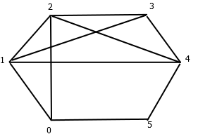
Figure 1: A graph with maximum clique

For example Figure 2 represents a graph($G$) of six vertices, The $k$-clique problem asks us to determine if the graph $G$ contains the the clique of size $k$ or not, and if it does, output the vertices forming the clique. If $k=4$ the output will be 1234, If $k=3$ output will be $(0,1,2),(1,2,4),(2,3,4)$.

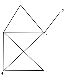
Figure 2: A 6 node undirected graph

2.2 Grover’s Algorithm

Grover’s algorithm[4] is based on amplitude amplification of the basis state which finds an element in an unsorted list. It runs in time O$(\sqrt{N})$, where $N$ is the number of elements in the list. The generalized structure of Grover’s algorithm is shown in Figure 3.

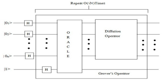
Figure 3: Generalized circuit for Grover’s algorithm

More elaborately, The steps of the Grover’s algorithm are as follows:

Initialization: The first step of the algorithm is state preparation. the initial state is prepared in an equal superposition over the entire Hilbert space using Hadamard gate (H). There are other methods too for initializing the input qubits like, Dicke state or W state that will be discussed next.

Dicke State:

Dicke state [22] is a quantum state preparation technique that limits the total Hilbert spaces by using some hammimg weight. A $n$-qubit quantum state $\ket{\psi_{n}}$ can be expressed as the superposition of $2^{n}$ orthonormal basis states. $\ket{D^{n}_{k}}$ is the $n$-qubit state, which is the equal superposition state of all $n\choose k$ basis states of weight $k$. For example,$\ket{D^{3}_{1}}=\sqrt{\frac{1}{3}}(\ket{001}+\ket{010}+\ket{100})$. Dicke state needs only polynomial number of elementary gates to prepare and have $n\choose k$ active basis states, which can be exponential in $n$ when $k=\theta(n)$. The construction of Dicke state $\ket{D^{4}_{3}}$ [23] is portrayed in Figure 4.

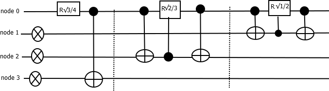
Figure 4: Circuit for $\ket{D^{4}_{3}}$

W State:

W state is a special case of the Dicke state. W state is a Dicke state with Hamming weight 1, such as $\ket{W}=\sqrt{\frac{1}{n}}(\ket{100...0}+\textperiodcentered\textperiodcentered\textperiodcentered+\ket{01...0}+\ket{00...01})$. The implementation of the W-state preparation follows from the article [24]. The circuit size and depth of W state preparation is less than Dicke state. The circuit for the W state preparation circuit for 6 qubits is shown in Figure 5. The output of this circuit is the superposition of the six states $\ket{100000}+\ket{010000}+\ket{001000}+\ket{000100}+\ket{000010}+\ket{000001}$. Limitation of W state is that it only works when clique size in $n-1$.

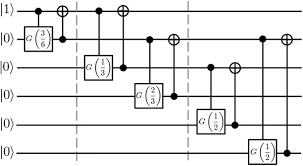
Figure 5: circuit for ${W_{6}}$

Oracle: Grover’s algorithm works with a unitary operator $O$ called the oracle function, that add a negative phase to the solution states. The functional view of Grover’s Search Algorithm is presented here. $\exists$ function oracle $(O)$ such that

$$O\ket{x}=\begin{cases}-\ket{x},&\text{if {x} is Marked}\\ \ket{x},&\text{otherwise}\end{cases}$$

This oracle will be a diagonal matrix, where the entry that correspond to the marked item will have a negative phase.

Amplitude Amplification: We need to perform the inversion about the average of all amplitudes of quantum state for an optimal number of iterations to make the amplitude of the marked state large enough so that it can be obtained from a measurement with probability close to 1.

Number of Iterations: Iterations of Grover’s algorithm are the number of times that the oracle and amplification stages are performed. Each iteration of the algorithm increases the amplitude of the marked state by $O(\sqrt{1/N})$. Grover’s search algorithm requires $\sqrt{N/M}$ iterations to get the probability of one of the marked states $M$ out of total $N$ number of states set. Therefore, optimal number of iterations are the key for getting proper result.

Diffusion operator: This procedure amplifies the amplitude of the marked item, and shrinks the other item’s amplitudes, so that measuring the final state will return the right item with near certainty. The generalized matrix representation of the diffusion operator is shown in Table 1. A six-qubit diffusion operator is also presented in Table 1. As shown in six-qubit diffusion operator, a 6-qubit Toffoli gate is required. Therefore, for $n$-qubit diffusion operator, $n$-qubit Toffoli gate is needed. This $n$-qubit Toffoli gate needs to be realized into one-qubit or two-qubit gates. While decomposing the $n$-qubit Toffoli gate, if the depth and the ancilla qubits increase arbitrarily then the run-time complexity of the algorithm also increases, which is undesirable.

Table 1: Diffusion Operator

Six-qubit Diffusion Circuit	Generalized Matrix Representation
	$\begin{pmatrix}-1+\frac{2}{N}&\frac{2}{N}&\ldots&\frac{2}{N}\\ \frac{2}{N}&-1+\frac{2}{N}&\ldots&\frac{2}{N}\\ \vdots&\vdots&\ddots&\vdots\\ \frac{2}{N}&\frac{2}{N}&\ldots&-1+\frac{2}{N}\end{pmatrix}$

2.3 Multi-controlled Toffoli Decomposition with Intermediate Qudits

This section starts with the discussion of qudit technology followed by Toffoli decomposition. [17]

2.3.1 Qudit

Qudit technology [25] is emerging as an alternative for quantum computation and quantum information science. Qudits provide a larger state space to store and process information and can do multiple control operations simultaneously. These features reduces the circuit complexity. Traditionally, quantum computation is expressed in terms of quantum bits, or qubits. We designate these two basis states as $\ket{0}$ and $\ket{1}$ and can represent any qubit as
$\psi=\alpha\ket{0}+\beta\ket{1}$
with $|\alpha^{2}+\beta^{2}|=1$. A qudit is the unit of quantum information for d-ary quantum systems. Qudit states can be expressed by a vector in the d-dimensional Hilbert space $H_{d}$. The vector space is the span of orthonormal basis vectors $\ket{0},\ket{1},\ket{2},\dots\ket{d-1}$. N qubits can be expressed as $\frac{N}{\log_{2}d}$ qudits. This reduces runtime of the algorithm by a $\log_{2}d$ factor. Qudit state can be described as
$\psi=\alpha_{0}\ket{0}+\alpha_{1}\ket{1}+\alpha_{2}\ket{2}+\dots\alpha_{d-1}\ket{d-1}$.
The state of a qudit is transformed by qudit gates Some useful gates of qudit systems are discussed next.[26]

Generalized CNOT gate

For d-ary quantum systems, the binary two-qubit CNOT gate is generalized to
$C_{X,d}\ket{x}\ket{y}=\ket{x}\ket{(y+1)\mod d}$
only if $x=d-1$ and otherwise = $\ket{x}\ket{y}$.

Generalized $n$-qudit Toffoli gate

We extend the generalized CNOT further to operate over $n$ qudits as a generalized $n$-qudit Toffoli gate $C^{n}_{X,d}$. For $C^{n}_{X,d}$ , the target qudit is incremented by 1 mod donly when all the $n-1$ control qudits are $d-1$.

2.3.2 n-qubit Toffoli Decomposition

Toffoli gate is the central building block of several quantum algorithms. Since the Toffoli involves 3-body interactions, it cannot be implemented naturally in a real quantum devices. Toffoli gate can be constructed by decomposing it into single and two qubit gates. For example CNOT gates require 6 such gates plus 10 single qubit gates;[27] For generalized Toffoli gates the resources increase rapidly, requiring $O(n^{2})$ two-qubit gates. Toffoli gates can be constructed efficiently using fewer resources than previous designs with the help of intermediate qudits [25].
The Figure 6 shows the docomposition of generalized Toffoli gate [17] in any finite dimensional quantum system or d-ary quantum systems. Target qudit is incremented ($X_{d}$ operation) when two-controlled qudits are both $\ket{d-1}$. First, a $\ket{d-1}$ controlled $X^{+1}_{d+1}$ operation increment the target qudit by $1\ mod\ (d+1)$. This changes the value of the second qudit to $\ket{d}$ if and only if the first and the second qudits were both $\ket{d-1}$. Then, a $\ket{d}$ controlled $X_{d}$ gate is applied to the target qudit. Therefore, $X_{d}$ is executed only when both the first and the second qudits are $\ket{d-1}$. The controls are reinstated to their original states by a $\ket{d-1}$ controlled $X^{-1}_{d+1}$ gate, which reverses the effect of the first gate. Next we shall apply this technique to decompose the 2-controlled, 3-controlled, 4-controlled and 5-controlled Toffoli gates.

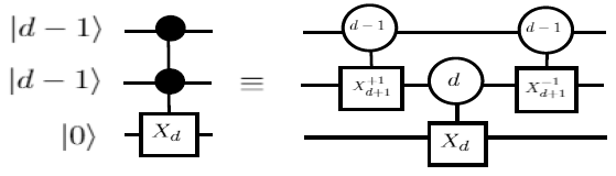
Figure 6: Generalized Toffoli in d-ary quantum systems

The generalized Toffoli gate decomposition as shown in the Figure 6 has been used for the decomposition of 2-controlled, 3-controlled, 4-controlled and 5-controlled Toffoli gates, which are used as examples for the circuit construction of clique problem in subsequent sections. The Figure 7 shows the decomposition of a 2-controlled Toffoli gate. Second qubit is incremented if the first control qubit is 1. $x^{+1}_{3}$ is modulo 3 increment gate, that increments the value of the second qubit. Finally last qubit is flipped is the control qubit is 2. The qubits values are uncomputed to their initial value.

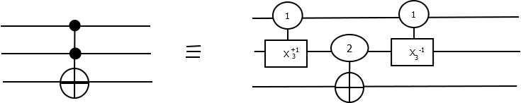
Figure 7: 2-controlled Toffoli Gate Decomposition

The Figure 8 shows the decomposition of a 3-controlled Toffoli gate. Third qubit is incremented if the first control qubit is 1. $x^{+1}_{3}$ is modulo 3 increment gate, Second qubit is incremented if third qubit is 2. The target qubit is incremented if 2nd qubit is 2. The qubits values are uncomputed to their initial value.

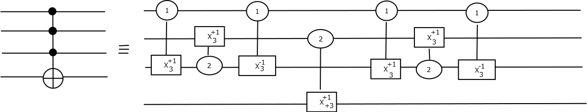
Figure 8: 3-controlled Toffoli Gate Decomposition

Further, the optimized 3-control Toffoli gate decomposition is given in Figure 9, where two generalized CNOT gates operating one after another on the same qudits are removed by applying the optimization rule as described in [28]

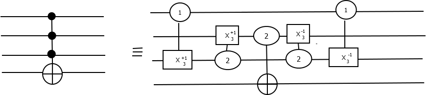
Figure 9: 3-controlled Toffoli Gate Optimized Decomposition

Decomposition of 4-controlled Toffoli gate is shown in Figure 10.

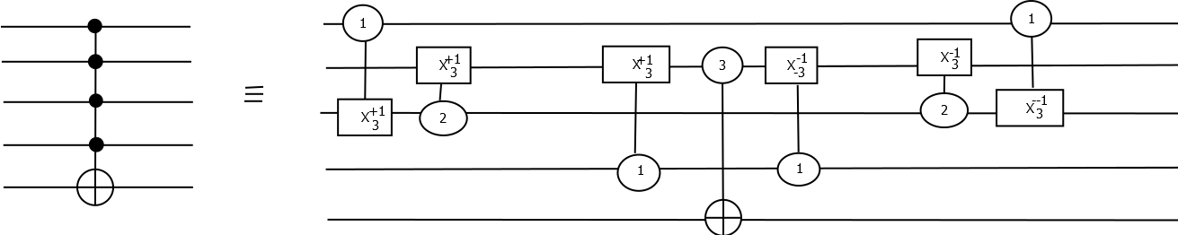
Figure 10: 4-controlled Toffoli Gate Optimized Decomposition

Decomposition of 5-controlled Toffoli gate is shown in Figure 11. The decomposition is done in the similar manner.

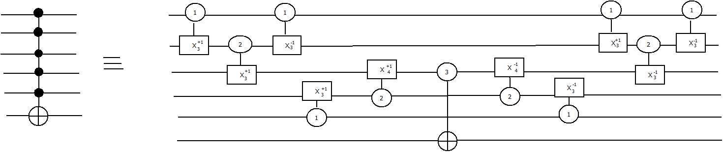
Figure 11: 5-controlled Toffoli Gate Decomposition

The optimized decomposition is shown in the Figure 12. As shown in Figure 12, to decompose 5-controlled Toffoli, we need to temporarily access 4-dimensional quantum systems or ququarts. In fact, in similar way for $n>4$, $n$-qubit Toffoli can be decomposed using in intermediate ququarts.

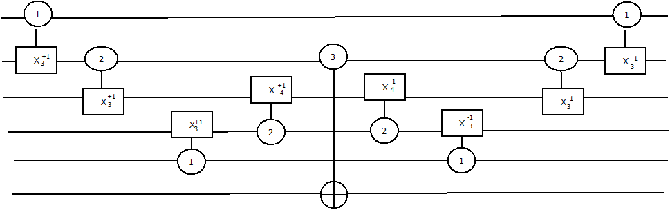
Figure 12: 5-controlled Toffoli Gate Optimized Decomposition

3 Quantum Circuit Construction for $k$-clique problem with Intermediate Qudits

Implementation of $k$-clique problem follows the method used in the article of Metwalli et al. [9]. For finding $k$-clique of a graph using Grover’s algorithm, we have to go through three steps namely input state preparation, oracle construction and amplification of the marked state. For the amplification of the marked states, we use Grover’s diffusion operator. Since Diffusion operator is problem independent, therefore we shall directly apply the operator as we have already exhibited in the Section 2. Therefore, only the first two steps have been detailed in the subsequent subsections.

3.1 Input State Preparation

In Grover’s algorithm, the states are prepared in an equal superposition of the whole Hilbert space using the H (Hadamard) gate. Initializing into full superposition needs only $n$ H gates and time complexity $O(1)$, since all H gates can be run simultaneously. Albeit, it unnecessarily searches the full Hilbert space. Here we use Dicke states and W state to limit the search spaces. If we want to search for a clique size four as shown in Figure 2, we shall limit the search space to only the subgraphs containing four vertices. The Dicke state preparation of the 4 nodes from 6 nodes is shown in Figure 4. After applying Dicke state circuit the input states will be the superposition of
$\ket{\psi}=\frac{1}{\sqrt{2}}\ket{011011}+\ket{011110}+\ket{001111}+\ket{011101}+\ket{111010}+\ket{111100}+\ket{010111}+\ket{101101}+\ket{110011}+\ket{101011}+\ket{110110}+\ket{101110}+\ket{111001}+\ket{110101}+\ket{100111}$.

3.2 Oracle Construction for $k$-clique

For finding a clique in a given graph, we have to check the total number of edges and vertices. Each node of the graph is represented by a qubit and the edges between them is checked using one or more multi-controlled Toffoli ($n$-qubit Toffoli) gates connecting respective qubits. Number of nodes are also tested using one or more multiple-controlled Toffoli ($n$-qubit Toffoli) gates. For the physical realization of Toffoli gate, it is decomposed into several 1-qubit or 2-qubit gates. Hence, the increasing number of Toffoli gates increase the circuit depth and size. In this work, we try to decompose these $n$-qubit Toffoli gates with intermediate higher dimensional qudits (qutrits or ququarts) for better circuit robustness.

There are two variations of this oracle one is Checking-based and another is Increment-based as discussed in the article [9]. Each oracle is detailed in the subsequent subsections.

3.2.1 Checking-based Oracle

In Checking-based oracle, there is an edge counter and a node counter. Each $n$-qubit Toffoli gates connecting the qubits represent one edge. When an edge is encountered, the value of the edge counter is increased by one. After all edges have been counted, the results are checked. If we want to find the clique of size 4 in graph $G$ as in Figure 2, then after applying $n$-qubit Toffoli gates, we need to check that we have precisely six edges (binary equivalent is $110_{2}$). We need $\log{k\choose 2}$ qubits to represent the edge counter. We require a 3 qubit counter here that can count up to 7 that is ($111_{2}$). We need an edge flag to check the value of the edge counter. Similar process is used to count the nodes using node counter. If the node counter contains the correct value then we may claim that a clique of size $k$ is found. The following Figure 13, 14 and 15 shows Checking-based oracle of the graph of Figure 2. The graph $G$ has nine edges as well as six nodes. The Figure 13 shows the oracle for checking the edges of a complete sub-graph of size 4. The Figure 14 shows the oracle for checking the node count. Three ancilla qubits are used here for counting six edges and four nodes.

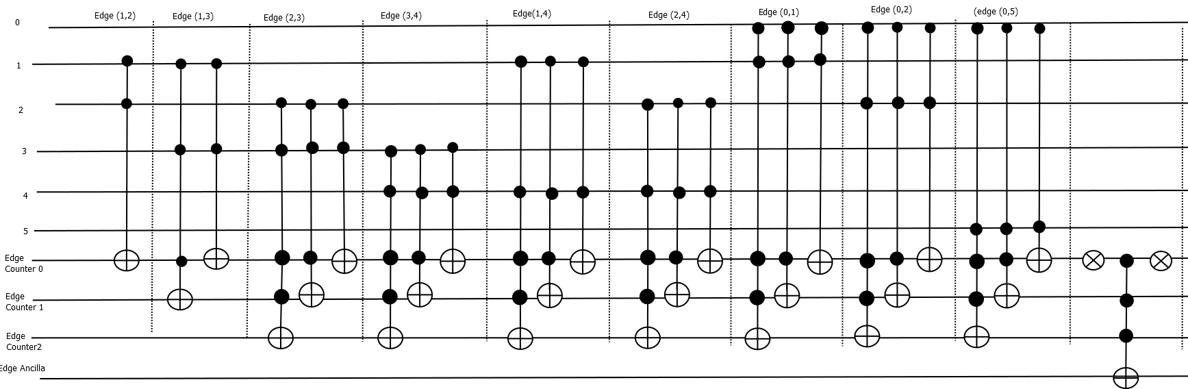
Figure 13: Checking-based edge oracle

Figure 14: Checking-based node oracle

If both the node flag and edge flag are high, then the target qubit is flipped. Figure 15 shows the whole procedure.

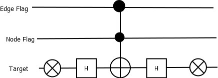
Figure 15: Checking-based node oracle

3.2.2 Incremental-based Oracle

For incremental-based oracle, an increment operator is applied. There is an one qubit edge flag. The edge flag becomes 1 if and only if an edge exists between two nodes. Edge flag is then used as a control qubit for an increment circuit that adds 1 every time it finds an edge. The following Figure 16 shows Incremental-based oracle of the graph of Figure 2. The graph $G$ has a sub-graph of six edges as well as four nodes. Hence, it contains a clique of size 4.

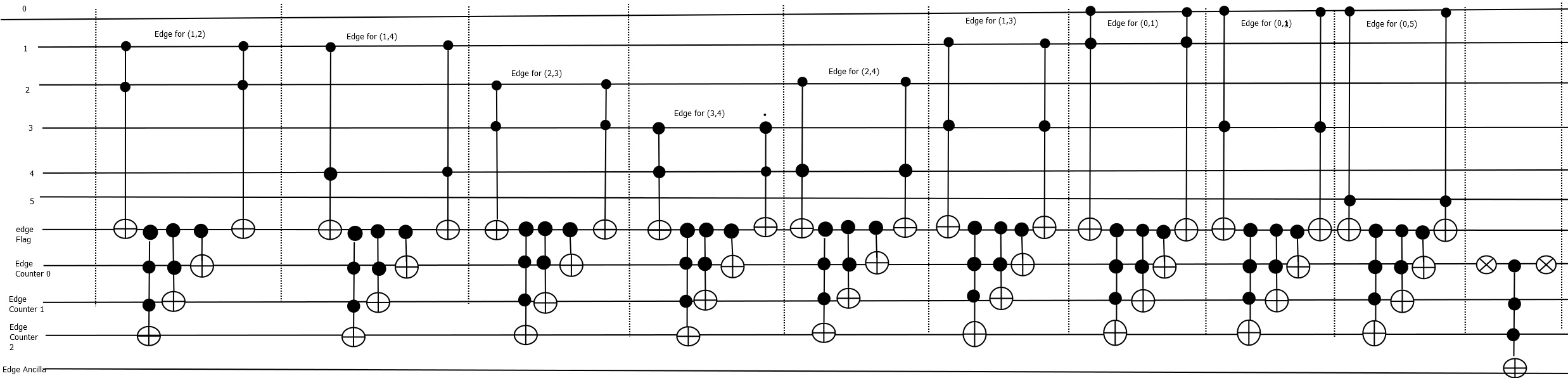
Figure 16: Increment-based edge oracle

The Figure 16 shows the Incremental-based oracle for counting six edges. The Figure 17 shows the Increment-based oracle for counting four nodes. The size of both the node counter and edge counter is 3.

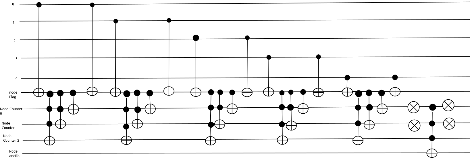
Figure 17: Increment-based node oracle

If the both node flag and edge flag are high then the target qubit is flipped as we can observe in the Figure 15. As we can observe from the Figure 13, 14, 16 and 17, a significant number of Toffoli gates has been used for the construction of these oracular circuits. Implementation of these large number of Toffoli gates increases circuit depth accordingly as detailed in the article [9], which makes the circuit impossible to implement in the real devices. Hence, the Toffoli gates are decomposed using intermediate qudit gates as discussed in section 2. This decomposition technique using qudit gates reduces the size and depth of the circuit remarkably as shown in the Figure 7, 9, 12.

Oracle Construction for $k$-clique Problem

The automated and generalized algorithm of quantum circuit synthesis for $k$-clique problem is discussed here. $k$-clique problem finds a clique of size $k$ in a graph. The steps of the circuit synthesis for $k$-clique are shown below:
Input : Graph $G(V,E)$, Size of the clique to be searched that is $k$
Output: Clique of size $k$

• Step 1: The total number of vertices are the input qubits of the circuit. Input states are prepared using Dicke state, W state or Hadamard gates.

• Step 2: Increment-based oracle or Checking-based oracle is used to count the number of nodes and edges of a sub-graph of size $k$. Edge counter should have the value $k\choose 2$ and node counter should have the value $k$. An edge flag is used to detect the correct value of the edge counter and a node flag is used to detect the correct value of the node counter.

• Step 3: If both the edge flag and node flag matches then a clique of size $k$ is found.

Oracle Construction for Maximum Clique Problem

The automated and generalized algorithm of quantum circuit synthesis for maximum clique problem is discussed here. maximum clique problem finds clique in a graph with maximum cardinality. The algorithm starts with finding clique of size $k$ = $n$ ($n$ is the total number of vertices of the graph) using the oracle of $k$-clique. If a clique is found, it is the maximum clique of the graph. Otherwise, a clique is searched for size $n-1$. The process continues up to $n=2$.
The steps of the circuit synthesis for MCP are shown below:
Input : Graph $G(V,E)$
Output: Maximum Clique of the graph

• Step 1: Algorithm for finding $k$-clique is used for searching clique of size $n$, where the number vertices of the given graph are $k$.

• Step 2: If a clique is found, then exit from the process.

• Step 3: If clique is not found, then clique size $n$ is reduced to $n-1$ and repeat the whole process from step 1.

• Step 4: At each iteration, the value of $n$ is reduced by 1 $(n,n-1,n-2,n-3,\dots,2)$ until a clique is found.

If we take a look at the Figure 2, there are 6 nodes and 9 edges. The maximum clique problem starts with $k=6$. A complete graph of 6 nodes contains $6\choose 2$, 15 edges. But the graph does not have 15 edges. Hence, next we try to find the clique of size $k=5$. A complete graph of 5 nodes contains $5\choose 2$, that means 10 edges. But the graph has only 9 edges. Hence, we move to the next iteration of searching with the clique size $k=4$. We find the total edge as 6 for 4 vertices in a subgraph. We stop the searching process and conclude that the maximum clique size of the graph is 4 of Figure 2.

4 Implementation Results and Analysis

The behaviour of a quantum algorithm can be realized by a simulator on a classical computer. Simulator sense how the quantum circuit may be implemented on a real quantum computer. The circuit for $k$-clique problem is simulated on Google Colaboratory platform [29].

4.1 Simulation with full Hilbert space

The oracle circuit for $k$-clique problem for the graph shown in Figure 2 has been implemented. Here, we have 6 qubit lines for inputs, there can be a total of $2^{6}=64$ different qubit combinations as $\ket{000000}$, $\ket{000001}$, $\dots$, $\ket{111111}$ after applying Hadamard gate to all input qubits. Hence, the database on which Grover’s algorithm is applied contains 64 different elements.

4.1.1 Simulation using Checking-based oracle

Figure 13, 14, shows the complete gate-level synthesis of Grover’s circuit for the 4-clique problem. It is to be noted that all the Toffoli or multi-controlled Toffoli gates are decomposed with intermediate qudits before performing the simulation procedure. The simulation steps required for the synthesis are as follows:

1. The oracle checks whether four vertices are connected with six edges or not. It then inverts the amplitude of the solution state for which the four vertex combination forms a sub graph with six edges. The solution state for this case is $\ket{011110}$,

2. The output of the oracle is acted upon by the Grover’s diffusion operator as shown in Figure 18. The diffusion operator amplifies the amplitude of the marked solution state.

3. Steps 1 and 2 constitute the Grover’s operator for the Grover’s search algorithm. Hence, these two steps are repeated $\dfrac{\pi}{4}\sqrt{\frac{64}{1}}$ times. (For an $N$ item database with $M$ number of known solutions [4], Grover’s iteration must be repeated $\dfrac{\pi}{4}\sqrt{\dfrac{N}{M}}$ times in order to obtain a solution). If our number of solutions are not previously known [30, 31, 32, 33, 34, 35], therefore we need to consider a tricky method for the iterations without any asymptotic penalty. As per [36], we need to start with a single application of the Grover Iterate. If the marked state is not found, repeat the Grover’s algorithm with a number of iterations which is $6$ times the previous number.

The resultant output after applying Grover’s operator $\dfrac{\pi}{4}\sqrt{1}$ $\sim$ $O(1)$ time is shown in Figure 18, where the amplitude of the solution state has been amplified. The location of the solution state is $\ket{011110}$, which is the vertex combination in an example graph of Figure 18 that forms clique with high probability. The circuit for clique size three has been simulated. The marked state $\ket{011110}$ is in high amplitude as shown in the output Figure 18, which depicts that $1$, $2$, $3$ and $4$ form a square. Similarly, the simulation of Increment-based oracle can be performed.

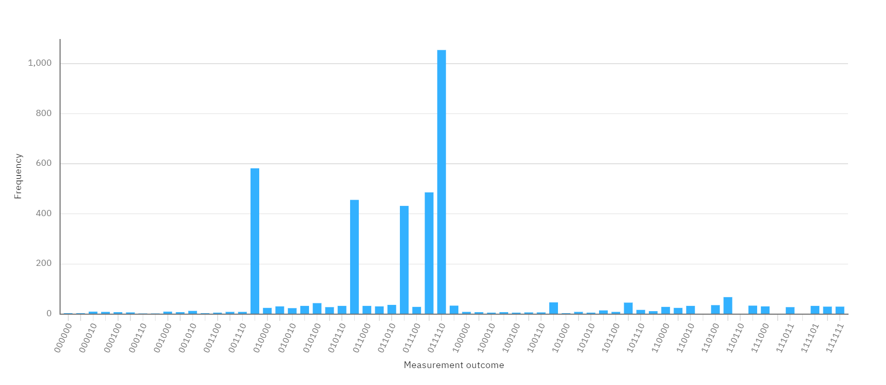
Figure 18: Ideal simulation of Checking-based oracle

4.1.2 Triangle finding problem using Dicke state preparation

In similar way, the implementation result of applying Checking-based oracle and Increment-based oracle in Google Colaboratory platform for finding a traingle in the graph in Figure 19 is shown in the Figure 20 and Figure 21. The input state preparation is used as Dicke state for the both oracle.

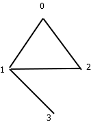
Figure 19: One Triangle

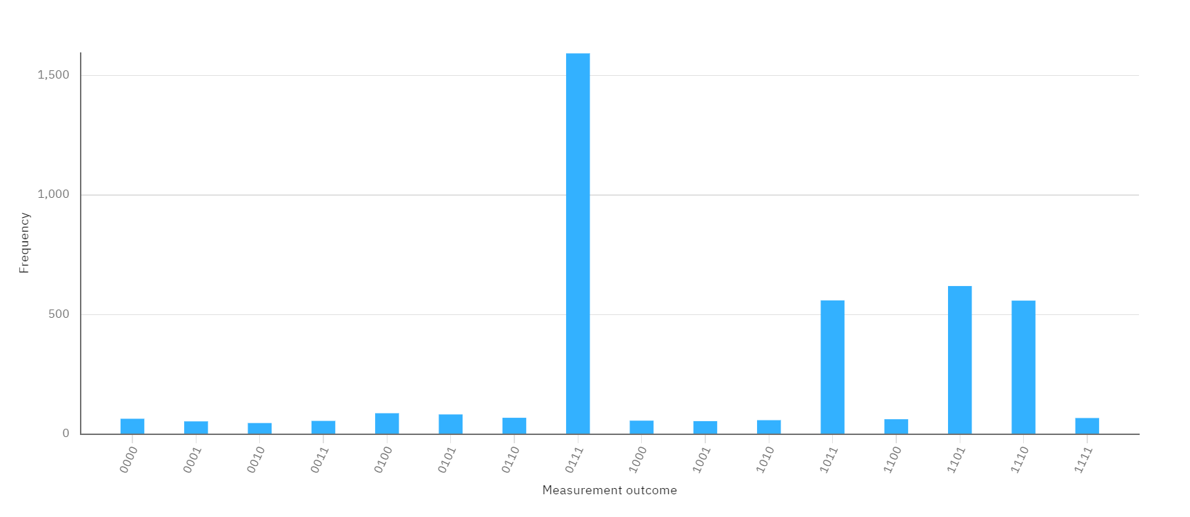
Figure 20: Output of Checking-based oracle for finding triangle

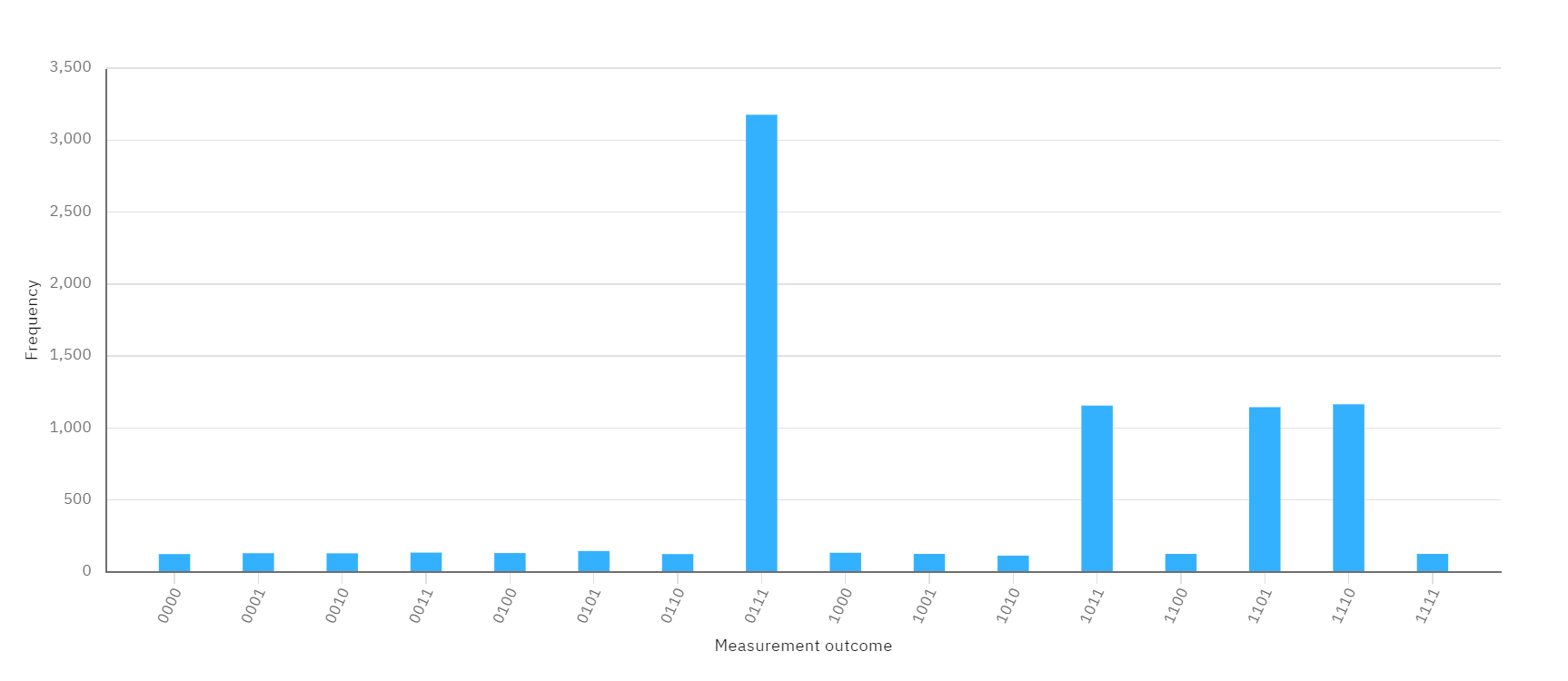
Figure 21: Output of Increment-based oracle for finding triangle

4.2 Circuit Cost Analysis

In order to test the efficiency of our implementation, we compared various combinations of the problem variables with the state-of-the-art problem. The comparison is based on the gate count (size) and the depth of the circuit proposed in the state-of-the-art article and the gate count (size) and the depth after applying the Toffoli decomposition with intermediate qudit technique. The circuit cost and depth have been analysed for both of the approaches i.e., Checking-based and Increment-based oracle. Before that let’s discuss about the cost of multi-controlled Toffoli decomposition with intermediate qudits.

4.2.1 Cost of Decomposed Toffoli Gate

As discussed Multi-controlled Toffoli gates can not be directly used in real quantum devices. To map those gates, it needs to be decomposed into several 1-qubit and 2-qubit gates. The circuit depth grows with the number of Toffoli controls when the MCT gate is implemented on the IBM Q devices. The total number of elementary gates required to map one Toffoli gate is 15 and the depth is 12 as shown in Figure 22. But if we use the decomposition technique that is shown in the Figure 9, we can observe that the Toffoli gates can be decomposed using only three 2-qutrit gates and the depth is also three. Hence, we can observe a significant improvement in terms of the cost and depth of the circuit. Table 2 shows Multi-controlled Toffoli gate variations with total number of gates needed to implement it using conventional method and using intermediate qudit.

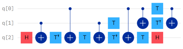
Figure 22: Decomposed Toffoli (Circuit Depth 12, T-count 7, CNOT count 6, H count 2).

Total number of 1-qubit, 2-qubit gates required to realize Toffoli gate is given in Table 2. As we observe from the Table 2 that the total number of gates to map one Toffoli gate is 15. Using the Toffoli decomposition technique we can reduce it. The total number of Toffoli gate for different state preparation techniques and the corresponding cost and depth comparison of the circuit is shown in the Table 3.

Table 2: Toffoli gate cost comparison using qubit and qudit gates

Decomposition technique	Number of control	size	Depth	1-qubit gates	2-qubit gates	2-qudit gates
Standard [9]	2	15	12	9	6	0
Intermediate Qudit	2	3	3	0	0	3
Standard [9]	3	27	22	14	13	0
Intermediate Qudit	3	5	5	0	0	5
Standard [9]	4	77	60	48	29	0
Intermediate Qudit	4	7	7	0	0	7

The total number of NOT, CNOT and Toffoli gates required for finding triangle in an arbitrary graph is shown in the Table 2 of the article [9].

Table 3: Toffoli count for Checking-based oracle

Method used	State Preparation	Total	Size	Depth
Standard [9]	Hilbert	63	945	756
Intermediate Qudit	Hilbert	63	189	189
Standard [9]	Dicke	18	270	216
Intermediate Qudit	Dicke	18	54	54

The Toffoli gate cost for Increment-based oracle for different state preparation techniques is given in the Table 4.

Table 4: Toffoli count for Increment-based oracle using qutrit

Method used	State Preparation	Total	Size	Depth
Standard [9]	Hilbert	48	720	576
Intermediate Qudit	Hilbert	48	144	144
Standard [9]	W state	8	120	96
Intermediate Qudit	W state	8	24	24
Standard [9]	Dicke state	26	390	312
Intermediate Qudit	Dicke state	26	78	78

As we can observe from the Table 4 that the size and depth of the circuit get reduced if we use higher dimensional Toffoli decomposition technique.

4.2.2 Total Cost for clique problem

Quantum circuit becomes difficult to implement on hardware if the number of gates of the circuit is very high because of its erroneous behaviour. Hence we have to find the circuit size and the depth of the circuit implementations for two kind of oracles with different state preparation techniques. In the Toffoli decomposition technique we have first identified the total number of multi controlled Toffoli gates required to implement the circuit. Each Toffoli gate is replaced with the equivalent decomposed circuit with intermediate qudit. Total depth and size is of one decomposed circuit is multiplied with the number of Toffoli gates and finally added to the size and depth of the circuit. A n-qubit Toffoli gate can be decomposed into a $\log_{2}n$ depth with no ancilla qubits. For example let us assume we need 14 $C^{\otimes 2}$NOT gates, 3 $C^{\otimes 3}$NOT gates and 1 $C^{\otimes 4}$NOT gates. For one $C^{\otimes 2}$NOT gate, both the decomposed circuit size and the depth using intermediate qudit are 3. Therefore both the total size and the depth for implementing 14 $C^{\otimes 2}$NOT gates are 42. Similarly both the total size and the depth for implementing 3 $C^{\otimes 3}$NOT gate are 15. Both the total size and depth for implementing 1 $C^{\otimes 4}$NOT gate are 7. Hence we can conclude that we are getting a exponential improvement over the depth of the circuit. The six tables listed in this section below compare the cost and the depth of the circuit while using standard decomposition and an intermediate qudit decomposition technique. We have taken four different graphs and we find a triangle in every graph. The cells marked with ’yellow’ color shows the results of the circuit size and the depth using higher dimensional decomposition technique.
Table 5 and Table 6 show the circuit parameters for implementing Increment-based oracle using W state and Dicke state, where the number of marked state is chosen as 1 that means we are trying to find one triangle. Hence, while using Dicke or W state the optimal number of iteration will be 1, as $N=4$ and $m=1$.

Table 5: Total Gate count for Increment-based oracle using W state Preparation

Decomposition Method used	Type of graph	Number of qubits	1-qubit gates	2-qubit gates	Qudit gates	size	Depth
Standard [9]		10	314	193	0	507	354
Intermediate Qudit		10	33	41	108	182	145
Standard [9]		10	370	229	0	599	419
Intermediate Qudit		10	33	43	126	202	164
Standard [9]		10	426	265	0	691	484
Intermediate Qudit		10	33	45	144	222	183
Standard [9]		10	258	157	0	415	289
Intermediate Qudit		10	33	44	135	212	174

Table 6: Total Gate count for Increment-based oracle using Dicke state Preparation

Decomposition Method used	Type of graph	Number of qubits	1-qubit gates	2-qubit gates	Qudit gates	size	Depth
Standard [9]		10	488	337	0	825	593
Intermediate Qudit		10	30	41	108	181	149
Standard [9]		10	544	373	0	917	658
Intermediate Qudit		10	30	43	126	201	168
Standard [9]		10	600	409	0	1009	723
Intermediate Qudit		10	31	45	144	220	189
Standard [9]		10	432	301	0	733	528
Intermediate Qudit		10	30	44	135	209	180

Table 7 and Table 8 portray the decomposed circuit results while implementing Checking-based oracle using W state and Dicke state respectively.

Table 7: Total Gate count for Checking-based oracle using W state Preparation

Decomposition Method used	Type of graph	Number of qubits	1-qubit gates	2-qubit gates	Qudit gates	size	Depth
Standard [9]		9	324	205	0	529	331
Intermediate Qudit		9	34	17	81	131	106
Standard [9]		10	396	253	0	649	391
Intermediate Qudit		9	33	17	100	150	125
Standard [9]		9	468	301	0	769	471
Intermediate Qudit		9	34	17	116	166	141
Standard [9]		9	252	157	0	409	267
Intermediate Qudit		9	34	17	100	150	125

Table 8: Total Gate count for Checking-based oracle using Dicke state Preparation

Decomposition Method used	Type of graph	Number of qubits	1-qubit gates	2-qubit gates	Qudit gates	size	Depth
Standard [9]		10	474	361	0	835	595
Intermediate Qudit		10	30	17	107	154	134
Standard [9]		10	538	413	0	951	676
Intermediate Qudit		10	30	17	100	147	127
Standard [9]		10	600	409	0	1009	723
Intermediate Qudit		10	30	17	116	163	143
Standard [9]		10	410	309	0	719	518
Intermediate Qudit		10	30	17	106	153	133

Table 9 and Table 10 exhibit the circuit cost while implementing Checking-based oracle and increment-based oracle. The initial state is Full Hilbert space here. So for 4 qubits , $N=16$ and marked state $m=1$. So the optimal number of iteration is 3.

Table 9: Total Gate count for Checking-based oracle in Full Hilbert space

Decomposition Method used	Type of graph	Number of qubits	1-qubit gates	2-qubit gates	Qudit gates	size	Depth
Standard [9]		13	1047	413	0	1812	331
Intermediate Qudit		13	42	48	328	418	381
Standard [9]		13	1239	921	0	2160	1416
Intermediate Qudit		13	42	48	394	456	419
Standard [9]		13	1431	1077	0	2508	1659
Intermediate Qudit		13	42	48	468	558	521
Standard [9]		13	855	609	0	1464	942
Intermediate Qudit		13	42	48	394	456	419

Table 10: Total Gate count for Increment-based oracle in Full Hilbert space

Decomposition Method used	Type of graph	Number of qubits	1-qubit gates	2-qubit gates	Qudit gates	size	Depth
Standard [9]		15	1731	909	0	2640	1284
Intermediate Qudit		15	42	175	510	727	688
Standard [9]		15	1599	1017	0	2616	1551
Intermediate Qudit		15	42	183	582	807	767
Standard [9]		15	1767	1125	0	2892	1674
Intermediate Qudit		15	42	185	600	827	787
Standard [9]		15	1263	801	0	2064	1041
Intermediate Qudit		15	42	183	582	807	767

As we know the circuit cost is defined by the number of gates used in the circuit and the depth of the circuit is the longest path of the circuit. Performance of the quantum circuit mainly depends on these two parameters. As we can observe from the Table 5, Table 6, Table 7, Table 8, Table 9 and Table 10, the oracular circuit is decomposed into 1-qubit and 2-qubit gates as per the state-of-the-art [9]. The total cost and the depth of are calculated using the conventional decomposition procedure [9]. Same graph is taken and the circuit is decomposed using intermediate qudits. We observe from the highlighted rows of the tables that the cost and depth of a circuit when it is decomposed in a higher dimensional qudits are sublimer than the conventional approach. For example if we look into the table 10, for the 1st graph, the size of the graph is 2640 if we use normal decomposition method, but if we apply the intermediate qudit decomposition method, we get the circuit size is 727. So we have a 72% improvement over the size of the circuit. Similarly the depth of the circuit is 688 using intermediate qudit decomposition as compared to 1284 using conventional decomposition method. So the depth of the circuit is reduced by 46%. In similar way, we have improved the size and the depth of the circuits for different graphs as shown in the tables.

4.3 Error Analysis

Any quantum system is susceptible to different types of errors such as decoherence, noisy gates. For a $d$-dimensional quantum system, the gate error scales as $d^{2}$ and $d^{4}$ for 1- and 2-qubit gates respectively [25]. Furthermore, for qubits, the amplitude damping error decays the state $\ket{1}$ to $\ket{0}$ with probability $\lambda_{1}$. For a $d$-dimensional system, every state in level $\ket{i}\neq\ket{0}$ has a probability $\lambda_{1}$ of decaying. In other words, the usage of higher dimensional states penalizes the system with more errors. Nevertheless, the effect of these errors on the used decomposition of Multi-controlled Toffoli gate has been studied by Saha et al. [17]. They have shown that although the usage of intermediate qudits lead to increased error, the overall error probability of the decomposition is lower than the existing ones since the number of gates and the depth are both reduced. This interpretation is also applicable for our approach of solving clique problem. Hence, we claim that our solution for clique problem with intermediate qudit is more superior in terms of error-efficiency as compared to [9].

4.4 Time Complexity Analysis

The time complexity depends on the number of iterations in Grover’s algorithm, the initial state preparation (in case of limited Hilbert space search), different oracles and diffusion operators complexities. The oracle and the diffusion operator are repeated $\frac{\pi}{4}\sqrt{N/M}$ times, which depends on the size of the search space and the expected number of marked states. As detailed in the article [9] the complexity of the cost of preparing W states is $O(|V|)$ ,the cost of preparing the Dicke state is $O(k|V|)$ for $k$-clique problem. The circuit complexity of W state preparation is $O(logn)$. The complexity of the oracle for the entire Hilbert space is $O(log(k)+|E|+|V|)$. The complexity of the oracle when using initial state preparation to limit the search space is $O(log(k)+|E|)$. The total complexity is $O(\sqrt{\frac{{n\choose k}}{m}}\times(O(oracle)+O(diffusionoperator)))$, where $m=$ marked states and $k=$ clique size. If we use W state or Dicke state as initial state preparation, the complexity becomes $O(Statepreparation)+O(\sqrt{\frac{{n\choose k}}{m}}\times(O(oracle)+O(diffusionoperator)))$. The run-time complexity of the algorithm is reduced to logarithmic factor due to the Toffoli decomposition method applied to the circuit. As Maximum Clique Problem is an iterative problem and it depends on the size of $k$ we have not showed the time complexity of this problem.

5 Conclusion

In this article, we have proposed an improved quantum circuit for the clique problem with the help of higher-dimensional intermediate temporary qudits. We have analyzed the performance of the proposed approaches and the state-of-the-art approach from different perspectives, such as gate count, circuit size and circuit depth. Effect of error has also been analyzed on the circuit for using higher dimensional gates. The result of the cost analysis and error analysis shows that the circuit can have a lower gate count and depth than the state-of-the-art approach which leads to the lower error probability. The optimized circuit can be implemented in real quantum devices with lower depth and cost. The results are very promising which pave the way for circuit implementation of other computational problems in near future.

References

- [1] G. Hao, L. Gui-Lu, S. Yang, X. Xiao-Lin, A quantum algorithm for finding a hamilton circuit, Communications in Theoretical Physics 35 (4) (2001) 385.
- [2] G. Hao, L. Gui-Lu, L. Feng, Quantum algorithms for some well-known np problems, Communications in Theoretical Physics 37 (4) (2002) 424.
-
[3]
P. W. Shor, Polynomial-time
algorithms for prime factorization and discrete logarithms on a quantum
computer, SIAM Journal on Computing 26 (5) (1997) 1484–1509.
doi:10.1137/s0097539795293172.
URL http://dx.doi.org/10.1137/S0097539795293172 - [4] L. K. Grover, A fast quantum mechanical algorithm for database search, in: Proceedings of the Twenty-eighth Annual ACM Symposium on Theory of Computing, STOC ’96, ACM, New York, NY, USA, 1996, pp. 212–219. doi:10.1145/237814.237866.
- [5] F. Magniez, M. Santha, M. Szegedy, Quantum Algorithms for the Triangle Problem, arXiv e-prints (2003) quant–ph/0310134arXiv:quant-ph/0310134.
- [6] H. Buhrman, R. Špalek, Quantum verification of matrix products, in: Proceedings of the Seventeenth Annual ACM-SIAM Symposium on Discrete Algorithm, SODA ’06, Society for Industrial and Applied Mathematics, USA, 2006, p. 880–889.
- [7] A. Saha, A. Chongder, S. B. Mandal, A. Chakrabarti, Synthesis of vertex coloring problem using grover’s algorithm, in: 2015 IEEE International Symposium on Nanoelectronic and Information Systems, 2015, pp. 101–106. doi:10.1109/iNIS.2015.55.
-
[8]
M. Luo, X.-B. Chen, Y.-X. Yang, X. Wang,
Geometry of quantum computation with
qudits, Nature 4 (2014) 2045–2322.
doi:10.1038/srep04044.
URL https://doi.org/10.1038/srep04044 - [9] S. A. Metwalli, F. Le Gall, R. Van Meter, Finding small and large -clique instances on a quantum computer, IEEE Transactions on Quantum Engineering 1 (2020) 1–11. doi:10.1109/TQE.2020.3045692.
-
[10]
A. Sanyal Bhaduri, A. Saha, B. Saha, A. Chakrabarti,
Circuit
design for clique problem and its implementation on quantum computer, IET
Quantum Communication 3 (1) (2022) 30–49.
arXiv:https://ietresearch.onlinelibrary.wiley.com/doi/pdf/10.1049/qtc2.12029,
doi:https://doi.org/10.1049/qtc2.12029.
URL https://ietresearch.onlinelibrary.wiley.com/doi/abs/10.1049/qtc2.12029 - [11] A. Brouwer, J. Shearer, N. Sloane, W. Smith, A new table of constant weight codes, IEEE Transactions on Information Theory 36 (6) (1990) 1334–1380. doi:10.1109/18.59932.
-
[12]
S. Fortunato,
Community
detection in graphs, Physics Reports 486 (3) (2010) 75–174.
doi:https://doi.org/10.1016/j.physrep.2009.11.002.
URL https://www.sciencedirect.com/science/article/pii/S0370157309002841 -
[13]
J. Kempe, Quantum random
walks: An introductory overview, Contemporary Physics 44 (4) (2003)
307–327.
doi:10.1080/00107151031000110776.
URL http://dx.doi.org/10.1080/00107151031000110776 -
[14]
Y. Aharonov, L. Davidovich, N. Zagury,
Quantum random
walks, Phys. Rev. A 48 (1993) 1687–1690.
doi:10.1103/PhysRevA.48.1687.
URL https://link.aps.org/doi/10.1103/PhysRevA.48.1687 -
[15]
A. M. Childs, E. Farhi, S. Gutmann,
An example of the difference
between quantum and classical random walks, Quantum Information Processing
1 (1/2) (2002) 35–43.
doi:10.1023/a:1019609420309.
URL http://dx.doi.org/10.1023/A:1019609420309 - [16] A. Ambainis, Quantum walk algorithm for element distinctness, in: 45th Annual IEEE Symposium on Foundations of Computer Science, 2004, pp. 22–31. doi:10.1109/FOCS.2004.54.
-
[17]
A. Saha, R. Majumdar, D. Saha, A. Chakrabarti, S. Sur-Kolay,
Asymptotically
improved circuit for a -ary grover’s algorithm with advanced decomposition
of the -qudit toffoli gate, Phys. Rev. A 105 (2022) 062453.
doi:10.1103/PhysRevA.105.062453.
URL https://link.aps.org/doi/10.1103/PhysRevA.105.062453 -
[18]
R. Carraghan, P. M. Pardalos,
An exact algorithm for
the maximum clique problem, Oper. Res. Lett. 9 (6) (1990) 375–382.
doi:10.1016/0167-6377(90)90057-C.
URL https://doi.org/10.1016/0167-6377(90)90057-C -
[19]
P. R. J. Östergård,
A fast algorithm for the
maximum clique problem, Discrete Appl. Math. 120 (1–3) (2002) 197–207.
doi:10.1016/S0166-218X(01)00290-6.
URL https://doi.org/10.1016/S0166-218X(01)00290-6 - [20] E. Tomita, T. Seki, An efficient branch-and-bound algorithm for finding a maximum clique, in: Proceedings of the 4th International Conference on Discrete Mathematics and Theoretical Computer Science, DMTCS’03, Springer-Verlag, Berlin, Heidelberg, 2003, p. 278–289.
- [21] A. Bojić, Quantum algorithm for finding a maximum clique in an undirected graph, Journal of Information and Organizational Sciences 36 (2012) 91–98.
-
[22]
R. Prevedel, G. Cronenberg, M. S. Tame, M. Paternostro, P. Walther, M. S. Kim,
A. Zeilinger,
Experimental
realization of dicke states of up to six qubits for multiparty quantum
networking, Phys. Rev. Lett. 103 (2009) 020503.
doi:10.1103/PhysRevLett.103.020503.
URL https://link.aps.org/doi/10.1103/PhysRevLett.103.020503 - [23] A. artschi, S. Eidenbenz, L. Antoni, J. Jansson, C. Levcopoulos, Deterministic preparation of dicke states, in: Fundamentals of Computation Theory, Springer International Publishing, Cham, 2019, pp. 126–139.
-
[24]
D. Cruz, R. Fournier, F. Gremion, A. Jeannerot, K. Komagata, T. Tosic,
J. Thiesbrummel, C. L. Chan, N. Macris, M.-A. Dupertuis, C. Javerzac-Galy,
Efficient quantum algorithms
for GHZ and W states, and implementation on the IBM quantum computer,
Advanced Quantum Technologies 2 (5-6) (2019) 1900015.
doi:10.1002/qute.201900015.
URL https://doi.org/10.1002%2Fqute.201900015 -
[25]
P. Gokhale, J. M. Baker, C. Duckering, N. C. Brown, K. R. Brown, F. T. Chong,
Asymptotic improvements to
quantum circuits via qutrits, in: Proceedings of the 46th International
Symposium on Computer Architecture, ISCA ’19, Association for Computing
Machinery, New York, NY, USA, 2019, p. 554–566.
doi:10.1145/3307650.3322253.
URL https://doi.org/10.1145/3307650.3322253 -
[26]
A. Muthukrishnan, C. R. Stroud,
Multivalued logic
gates for quantum computation, Phys. Rev. A 62 (2000) 052309.
doi:10.1103/PhysRevA.62.052309.
URL https://link.aps.org/doi/10.1103/PhysRevA.62.052309 - [27] D. Große, R. Wille, G. W. Dueck, R. Drechsler, Exact multiple-control toffoli network synthesis with sat techniques, IEEE Transactions on Computer-Aided Design of Integrated Circuits and Systems 28 (5) (2009) 703–715. doi:10.1109/TCAD.2009.2017215.
- [28] F. L. Gall, Improved quantum algorithm for triangle finding via combinatorial arguments, in: 2014 IEEE 55th Annual Symposium on Foundations of Computer Science, 2014, pp. 216–225. doi:10.1109/FOCS.2014.31.
-
[29]
E. Bisong, Google
Colaboratory, Apress, Berkeley, CA, 2019, pp. 59–64.
doi:10.1007/978-1-4842-4470-8_7.
URL https://doi.org/10.1007/978-1-4842-4470-8_7 -
[30]
T. J. Yoder, G. H. Low, I. L. Chuang,
Fixed-point quantum
search with an optimal number of queries, Physical Review Letters 113 (21).
doi:10.1103/physrevlett.113.210501.
URL http://dx.doi.org/10.1103/PhysRevLett.113.210501 -
[31]
G. L. Long, Y. S. Li, W. L. Zhang, L. Niu,
Phase matching in
quantum searching, Physics Letters A 262 (1) (1999) 27–34.
doi:10.1016/s0375-9601(99)00631-3.
URL http://dx.doi.org/10.1016/S0375-9601(99)00631-3 - [32] G. Long, X. Li, Y. Sun, Phase matching condition for quantum search with a generalized initial state, Physics Letters A 294 (2002) 143–152.
-
[33]
L. Gui-Lu, General quantum
interference principle and duality computer, Communications in Theoretical
Physics 45 (5) (2006) 825–844.
doi:10.1088/0253-6102/45/5/013.
URL https://doi.org/10.1088/0253-6102/45/5/013 -
[34]
S. Jin, S. Wu, G. Zhou, Y. Li, L. Li, B. Li, X. Wang,
A query-based
quantum eigensolver, Quantum Engineering 2 (3) (2020) e49.
arXiv:https://onlinelibrary.wiley.com/doi/pdf/10.1002/que2.49, doi:https://doi.org/10.1002/que2.49.
URL https://onlinelibrary.wiley.com/doi/abs/10.1002/que2.49 -
[35]
L. Ding, T. Zhou,
Implementation of a
fixed-point quantum search by duality computer, EPL (Europhysics Letters)
126 (2) (2019) 20004.
doi:10.1209/0295-5075/126/20004.
URL https://doi.org/10.1209/0295-5075/126/20004 -
[36]
M. Boyer, G. Brassard, P. Høyer, A. Tapp,
Tight
bounds on quantum searching, Fortschritte der Physik 46 (4-5) (1998)
493–505.
doi:10.1002/(sici)1521-3978(199806)46:4/5<493::aid-prop493>3.0.co;2-p.
URL http://dx.doi.org/10.1002/(SICI)1521-3978(199806)46:4/5<493::AID-PROP493>3.0.CO;2-P