Linear Optimal Power Flow for Three-Phase Networks with Voltage-Dependent Loads in Delta Connections

Abstract

This paper proposes a linear approximation of the alternating current optimal power flow problem for multiphase distribution networks with voltage-dependent loads connected in both wye and delta configurations. We present a system of linear equations that uniquely determines the relationship between the power withdrawal/injection from a bus and that from a delta-connected device by employing assumptions required by a widely used linear model developed for networks with only wye connections and constant power load models. Numerical studies on IEEE test feeders demonstrate that the proposed linear model provides solutions with reasonable error bounds efficiently, as compared with an exact nonconvex formulation and a convex conic relaxation. We experimentally show that modeling delta-connected, voltage-dependent loads as if they are wye connected can yield contradictory results. We also discuss when the proposed linear approximation may outperform the convex conic relaxation.

I Introduction

Optimal power flow (OPF) refers to an optimization problem that aims to find an optimal operating point for a power grid while abiding by physical laws governing the electric power flow as well as various operational limits imposed on network components. OPF is often embedded in a variety of optimization problems that arise in the planning and operation of power grids (e.g., unit commitment and expansion planning problems), but the power flow equations that formulate the steady-state physics of power flow make OPF both nonconvex and NP-hard even for radial networks [1]. Because of OPF’s computational complexity and wide applicability, the past decade has seen an active line of research that attempts to reformulate OPF into a computationally tractable problem, especially as a convex relaxation and/or a linear approximation. For a comprehensive review of various OPF formulations, we refer readers to [2].

Most of the literature has focused on transmission grids that feature balanced OPF that can be treated like a single-phase network. OPF for distribution grids has received less attention because they are usually characterized by unidirectional power flow over a huge radial network, which makes their operations largely based on monitoring and controlling a small subset of network components, rather than by solving OPF. However, OPF in distribution grids becomes important as an increasing number of distributed energy resources introduce bidirectional power flow, which requires active controls based on OPF. Moreover, the single-phase models may not be directly applicable because of the unbalanced nature of distribution grids, which calls for tractable multiphase OPF formulations for distribution grids. In addition, it is important to model the voltage dependency of loads in distribution grids in order to employ conservation voltage reduction for reducing consumption [3]. Given the increasingly important role of OPF in distribution grids, ongoing efforts seek to develop an open-source framework that facilitates the implementation of OPF for distribution grids [4, 5].

For the unbalanced, multiphase OPF, semidefinite programming (SDP) relaxations have been proposed for networks with wye-connected constant-power loads [6, 7]. A linear approximation has also been proposed by ignoring line losses and assuming nearly balanced voltages [7]. The SDP relaxation is extended in [8] to networks with both wye- and delta-connected devices by introducing an additional positive semidefinite matrix that represents the outer product of bus voltages and phase-to-phase currents in the delta connection. In [9] the authors proposed an algorithm for achieving exactness of this SDP relaxation that adds a penalty term in the objective function. For voltage-dependent loads, approximate representations of ZIP loads were proposed in [10] and [11]. In this paper we focus on multiphase OPF for networks with delta-connected, exponential loads. The most related work is [12], which proposed a convex conic relaxation of exponential loads using power cones that can be added to an SDP relaxation of the multiphase OPF problem.

Convex conic relaxations have several advantages in that they provide lower bounds or even a globally optimal solution (for constant load models) to the nonconvex OPF problems and also are proven to be efficiently solvable by interior-point methods. In practice, however, they often suffer from numerical issues and show slow computation time when solving large-scale problems. This makes the convex conic relaxations difficult to be embedded in planning and operations problems with more features, for example, line switching and transformer controls.

Alternatively, we propose a linear approximation of multiphase OPF with exponential load models configured as either wye or delta connections. The proposed model uses the assumptions required by the linear model of [7] and provides a set of linear equations that uniquely determines the relationship between the power withdrawal/injection from a bus and that from a delta-connected device. This indicates that the proposed system of linear equations that formulates the delta connection is exact under the widely used assumptions, which is our main contribution in this paper. We numerically demonstrate that the proposed model provides solutions with reasonable error bounds (e.g., $<1\%$ on the voltage magnitude) much faster than the convex relaxation for three IEEE distribution feeders. A numerical experiment shows that the error of treating delta-connected, voltage-dependent loads as if they are wye-connected may become amplified as voltage dependency increases. We also identify when the linear approximation may outperform the convex conic relaxation.

This paper is organized as follows. Section II defines preliminaries on the network model and formalizes the multiphase alternating current (AC) OPF problem with only wye-connected, constant-power loads. Subsequently, its SDP relaxation and the linear approximation are described. In Section III, their extensions to the networks with delta-connected, voltage-dependent loads are explained and proposed. Section IV reports numerical results for three IEEE test systems, and Section V provides a summary of the paper.

II Preliminaries

Throughout this paper, calligraphic letters denote sets, and bold-faced letters denote vectors or matrices depending on the context. Complex numbers are denoted by non-bold, upper-case letters. For a matrix $\boldsymbol{A}\in\mathbb{C}^{n\times n}$, $\mbox{diag}(\boldsymbol{A})$ denotes a vector in $\mathbb{C}^{n}$ constructed by the diagonal elements of $\boldsymbol{A}$; we abuse notation and use $\mbox{diag}(\boldsymbol{a})$ for a vector $\boldsymbol{a}\in\mathbb{C}^{n}$ to represent a matrix in $\mathbb{C}^{n\times n}$ in which its diagonal is composed of $\boldsymbol{a}$ and the remaining off-diagonal elements are all zeros. For a complex vector or matrix $\boldsymbol{A}$, $\boldsymbol{A}^{H}$ denotes its conjugate transpose.

Let $(\mathcal{N},\mathcal{E})$ denote an undirected graph representing a distribution grid, where $\mathcal{N}$ and $\mathcal{E}$ denote the set of buses and lines, respectively. $\mathcal{N}$ is indexed with $\{0,1,\cdots,n\}$ for some integer $n$, where $0$ denotes the substation bus that serves as the slack bus in which the voltage is fixed and specified. Each line in $\mathcal{E}$ is indexed by a tuple $(e,i,j)$, where $e$ denotes an integer for indexing the line and $\{i,j\}\subseteq\mathcal{N}$ denote its two end buses. Most distribution grids involve three phases and are operated in radial (i.e., tree) structures, so we focus on the case where the graph is a tree (i.e., $(\mathcal{N},\mathcal{E})$ is connected and $|\mathcal{E}|=n$). Let $\mathcal{P}:=\{a,b,c\}$ denote the three phases of the network, and let $\mathcal{P}_{x}\subseteq\mathcal{P}$ be the phases of a network component $x$ (e.g., a line or a load).

For each bus $i\in\mathcal{N}$, let $V_{i\phi}$ denote the complex bus voltage at $i$ on phase $\phi\in\mathcal{P}$, and define $\boldsymbol{V}_{i}=[V_{i\phi}]_{\phi\in\mathcal{P}}$. For each line $(e,i,j)\in\mathcal{E}$, let $I_{eij\phi}$ (and $I_{eji\phi})$ represent the complex current flowing through the line from its $i$-end (and $j$-end) on phase $\phi\in\mathcal{P}$, and define $\boldsymbol{I}_{eij}=[I_{eij\phi}]_{\phi\in\mathcal{P}}$ (and $\boldsymbol{I}_{eji}=[I_{eji\phi}]_{\phi\in\mathcal{P}}$). As illustrated in Figure 1, the complex current is composed of complex series and shunt currents, each of which is denoted by $\boldsymbol{I}^{s}_{eij}=[I^{s}_{eij\phi}]_{\phi\in\mathcal{P}}$ and $\boldsymbol{I}^{sh}_{eij}=[I^{sh}_{eij\phi}]_{\phi\in\mathcal{P}}$, respectively (i.e., $\boldsymbol{I}_{eij}=\boldsymbol{I}^{s}_{eij}+\boldsymbol{I}^{sh}_{eij}$). The series impedance matrix and shunt admittance matrices of line $e$ are respectively denoted by ${\color[rgb]{0,0,0}\boldsymbol{Z}_{e}}=[{\color[rgb]{0,0,0}Z_{e\phi\phi^{\prime}}}]_{\phi,\phi^{\prime}\in\mathcal{P}}$, ${\color[rgb]{0,0,0}\boldsymbol{Y}^{sh}_{eij}}=[{\color[rgb]{0,0,0}Y^{sh}_{eij\phi\phi^{\prime}}}]_{\phi,\phi^{\prime}\in\mathcal{P}}$, and ${\color[rgb]{0,0,0}\boldsymbol{Y}^{sh}_{eji}}=[{\color[rgb]{0,0,0}Y^{sh}_{eji\phi\phi^{\prime}}}]_{\phi,\phi^{\prime}\in\mathcal{P}}$. We also define $\boldsymbol{S}_{eij}=[S_{eij\phi}]_{\phi\in\mathcal{P}}$ (and $\boldsymbol{S}_{eji}=[S_{eji\phi}]_{\phi\in\mathcal{P}})$ to represent the complex series power flowing through the line from its $i$-end (and $j$-end).

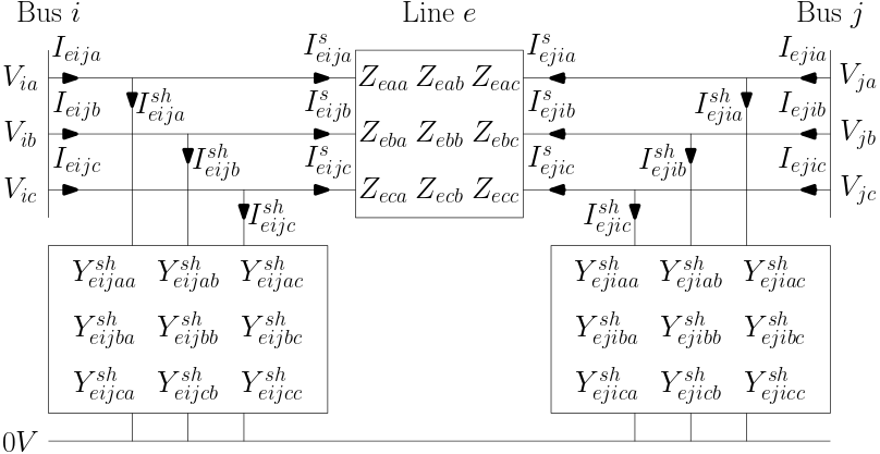
Figure 1: Notations for line $(e,i,j)\in\mathcal{E}$

A bus $i\in\mathcal{N}$ may be connected to multiple network components such as shunt devices, generators, and loads. Let $\mathcal{B}(i)$, $\mathcal{G}(i)$, and $\mathcal{L}(i)$ respectively denote the set of shunt devices, generators, and loads connected to the bus $i$; let $\mathcal{B},\mathcal{G},$ and $\mathcal{L}$ respectively denote the set of all shunt devices, generators, and loads in the network. Let $\boldsymbol{I}^{sh}_{s}=[I^{sh}_{s\phi}]_{\phi\in\mathcal{P}},s\in\mathcal{B}(i)$, $\boldsymbol{I}^{g}_{k}=[I^{g}_{k\phi}]_{\phi\in\mathcal{P}},k\in\mathcal{G}(i)$, and $\boldsymbol{I}^{b}_{l}=[I^{b}_{l\phi}]_{\phi\in\mathcal{P}},l\in\mathcal{L}(i)$ represent the current flowing from or to shunt devices, generators, and loads, respectively, as illustrated in Figure 2. A shunt device $s\in\mathcal{B}$ is characterized by its impedance matrix ${\color[rgb]{0,0,0}\boldsymbol{Y}^{sh}_{s}}=[{\color[rgb]{0,0,0}Y^{sh}_{s\phi\phi^{\prime}}}]_{\phi,\phi^{\prime}\in\mathcal{P}}$. For each generator $k\in\mathcal{G}$, its power output is denoted by $\boldsymbol{S}^{g}_{k}:=[S^{g}_{k\phi}]_{\phi\in\mathcal{P}}$. The output is controlled within its feasible region $\mathcal{S}_{k}$ that is usually specified by bounds on real and reactive power (i.e., $\mathcal{S}_{k}=\{\boldsymbol{p}_{k}+\mathrm{i}\boldsymbol{q}_{k}:{\color[rgb]{0,0,0}\underline{\boldsymbol{p}}_{k}}\leq\boldsymbol{p}_{k}\leq{\color[rgb]{0,0,0}\overline{\boldsymbol{p}}_{k}},{\color[rgb]{0,0,0}\underline{\boldsymbol{q}}_{k}}\leq\boldsymbol{q}_{k}\leq{\color[rgb]{0,0,0}\overline{\boldsymbol{q}}_{k}}\}$ for some constant vectors $\underline{\boldsymbol{p}}_{k}$, $\overline{\boldsymbol{p}}_{k}$, $\underline{\boldsymbol{q}}_{k}$, $\overline{\boldsymbol{q}}_{k}$$\in\mathbb{R}^{3})$. The electric power withdrawn from bus $i$ by load $l\in\mathcal{L}(i)$ is denoted by $\boldsymbol{S}^{b}_{l}=[S^{b}_{l\phi}]_{\phi\in\mathcal{P}}$ that is a function of the bus voltage, say, $f_{l}(\boldsymbol{V}_{i})$. The form of the function $f_{l}$ depends on how the load is modeled (e.g., constant power, constant impedance, exponential load) and configured (e.g., delta or wye). In this preliminary section, $f_{l}(\boldsymbol{V}_{i})$ is considered as a constant function $f_{l}(\boldsymbol{V}_{i})={\color[rgb]{0,0,0}\boldsymbol{S}_{l}^{0}}$ for its nominal power ${\color[rgb]{0,0,0}\boldsymbol{S}_{l}^{0}}$ since a majority of the previous literature on OPF assumes wye-connected constant power loads. Later in this paper, we consider a more general form of $f_{l}(\boldsymbol{V}_{i})$ that can model voltage-dependent load configured either as a wye or delta connection. Section III-B will discuss the general load modeling in detail.

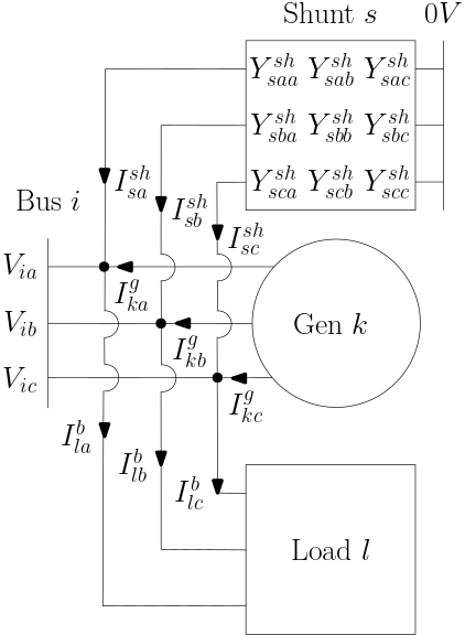
Figure 2: Notations for bus $i\in\mathcal{N}$

We consider each phase $a,b,c$ an integer $0,1,2$, respectively, so that for $\phi\in\mathcal{P}$, (i) $\phi^{+}$ refers to $(\phi+1)\bmod 3$ and (ii) $\phi^{-}:=(\phi+2)\bmod 3$. For example $a^{+}=b$ and $a^{-}=c$.

Power flows are governed by the following physical laws:

• Due to Ohm’s law, $\boldsymbol{V}_{i}-\boldsymbol{V}_{j}={\color[rgb]{0,0,0}\boldsymbol{Z}_{e}}\boldsymbol{I}^{s}_{eij}$, ${\color[rgb]{0,0,0}\boldsymbol{Y}^{sh}_{eij}}\boldsymbol{V}_{i}=\boldsymbol{I}^{sh}_{eij}$, and ${\color[rgb]{0,0,0}\boldsymbol{Y}^{sh}_{eji}}\boldsymbol{V}_{j}=\boldsymbol{I}^{sh}_{eji}$ for each line $(e,i,j)\in\mathcal{E}$, and ${\color[rgb]{0,0,0}\boldsymbol{Y}^{sh}_{s}}\boldsymbol{V}_{i}=-\boldsymbol{I}^{sh}_{s}$ for each bus $i\in\mathcal{N}$ and shunt device $s\in\mathcal{B}(i)$.

• Due to Kirchhoff’s current law, $\boldsymbol{I}^{s}_{eij}=-\boldsymbol{I}^{s}_{eji}$ for each line $(e,i,j)\in\mathcal{E}$, and for each bus $i\in\mathcal{N}$, $\sum_{(e,i,j)\mbox{ or }(e,j,i)\in\mathcal{E}}\boldsymbol{I}_{eij}=\sum_{s\in\mathcal{B}(i)}\boldsymbol{I}^{sh}_{s}+\sum_{k\in\mathcal{G}(i)}\boldsymbol{I}^{g}_{k}-\sum_{l\in\mathcal{L}(i)}\boldsymbol{I}^{b}_{l}.$

• Due to the power equation, for each line $(e,i,j)\in\mathcal{E}$, $\boldsymbol{S}_{eij\phi}=V_{i\phi}(I^{s}_{eij\phi})^{H}$ and $\boldsymbol{S}_{eji\phi}=V_{j\phi}(I^{s}_{eji\phi})^{H},\ \forall\phi\in\mathcal{P}$, and for each bus $i\in\mathcal{N}$, $\boldsymbol{S}^{g}_{k\phi}=V_{i\phi}(I_{k\phi}^{g})^{H},\ \forall k\in\mathcal{G}(i),\phi\in\mathcal{P}$ and $\boldsymbol{S}^{b}_{l\phi}=V_{i\phi}(I^{b}_{l\phi})^{H},\ \forall l\in\mathcal{L}(i),\phi\in\mathcal{P}$.

By eliminating current variables except $\boldsymbol{I}^{s}_{eij}$ and introducing auxiliary variables $\boldsymbol{L}_{eij}$ for $\boldsymbol{I}^{s}_{eij}(\boldsymbol{I}^{s}_{eij})^{H}$, $\boldsymbol{W}_{i}$ for $\boldsymbol{V}_{i}\boldsymbol{V}_{i}^{H}$, and $\boldsymbol{M}_{eij}$ for $\boldsymbol{V}_{i}(\boldsymbol{I}^{s}_{eij})^{H}$, the physical laws can be reduced to the following set of constraints, which is often referred to as a branch-flow model [7]:

$$\forall i\in\mathcal{N}_{{leaf}}:$$

$$\quad\boldsymbol{W}_{i}=\boldsymbol{V}_{i}\boldsymbol{V}_{i}^{H},$$ (1a)

$$\forall(e,i,j)\in\mathcal{E}:$$

$$\quad\left[\begin{array}[]{cc}\boldsymbol{W}_{i}&\boldsymbol{M}_{eij}\\ \boldsymbol{M}^{H}_{eij}&\boldsymbol{L}_{eij}\end{array}\right]=\left[\begin{array}[]{c}\boldsymbol{V}_{i}\\ \boldsymbol{I}^{s}_{eij}\end{array}\right]\left[\begin{array}[]{c}\boldsymbol{V}_{i}\\ \boldsymbol{I}^{s}_{eij}\end{array}\right]^{H},$$ (1h)

$$\quad\boldsymbol{V}_{j}=\boldsymbol{V}_{i}-{\color[rgb]{0,0,0}\boldsymbol{Z}_{e}}\boldsymbol{I}^{s}_{eij},$$ (1i)

$$\quad I^{s}_{eij\phi}=0,\ \forall\phi\notin\mathcal{P}_{e},$$ (1j)

$$\quad\boldsymbol{S}_{eij}=\mbox{diag}(\boldsymbol{M}_{eij}),$$ (1k)

$$\quad\boldsymbol{S}_{eji}=-\boldsymbol{S}_{eij}+\mbox{diag}({\color[rgb]{0,0,0}\boldsymbol{Z}_{e}}\boldsymbol{L}_{eij}),$$ (1l)

$$\forall l\in\mathcal{L}:$$

$$\quad\boldsymbol{S}^{b}_{l}={\color[rgb]{0,0,0}\boldsymbol{S}^{0}_{l}},$$ (1m)

$$\forall i\in\mathcal{N}:$$

$$\quad\sum_{(e,i,j)\mbox{ or }(e,j,i)\in\mathcal{E}}(\boldsymbol{S}_{eij}+\mbox{diag}(\boldsymbol{W}_{i}({\color[rgb]{0,0,0}\boldsymbol{Y}^{sh}_{eij}})^{H}))=$$

$$\quad\sum_{s\in\mathcal{B}(i)}\mbox{diag}(\boldsymbol{W}_{i}({\color[rgb]{0,0,0}\boldsymbol{Y}^{sh}_{s}})^{H})+\sum_{k\in\mathcal{G}(i)}\boldsymbol{S}^{g}_{k}-\sum_{l\in\mathcal{L}(i)}\boldsymbol{S}^{b}_{l},$$ (1n)

where $\mathcal{N}_{{leaf}}$ denotes the set of leaf buses.

II-A Multiphase AC OPF

Each generator $k\in\mathcal{G}$ incurs cost $C_{k}(\boldsymbol{S}^{g}_{k})$ for generating $\boldsymbol{S}^{g}_{k}\in\mathcal{S}_{k}$. OPF aims to minimize the total generation cost for satisfying the load while abiding by the physical laws, namely, Equations (1), as well as a set of operational constraints. These constraints include generation bounds, voltage bounds, and substation voltage level:

$$\boldsymbol{S}^{g}_{k}\in\mathcal{S}_{k},\ \forall k\in\mathcal{G},$$ (2a)

$${\color[rgb]{0,0,0}\underline{v}_{i\phi}^{2}}\leq\mbox{diag}(\boldsymbol{W}_{i})_{\phi}\leq{\color[rgb]{0,0,0}\overline{v}_{i\phi}^{2}},\ \forall i\in\mathcal{N},\ \phi\in\mathcal{P},$$ (2b)

$$\boldsymbol{W}_{0}={\color[rgb]{0,0,0}\boldsymbol{V}_{0}^{ref}(\boldsymbol{V}_{0}^{ref})^{H}},$$ (2c)

where ${\color[rgb]{0,0,0}\boldsymbol{V}_{0}^{ref}}$ denotes the specified voltage for the slack bus, ${\color[rgb]{0,0,0}\underline{v}_{i\phi}}$ and ${\color[rgb]{0,0,0}\overline{v}_{i\phi}}$ respectively denote the lower and upper bounds of voltage magnitude at bus $i$ on phase $\phi$, and $\mathcal{S}_{k}$ is the feasible power output region of generator $k\in\mathcal{G}$, which is defined as $\{\boldsymbol{p}_{k}+\mathrm{i}\boldsymbol{q}_{k}:{\color[rgb]{0,0,0}\underline{\boldsymbol{p}}_{k}}\leq\boldsymbol{p}_{k}\leq{\color[rgb]{0,0,0}\overline{\boldsymbol{p}}_{k}},{\color[rgb]{0,0,0}\underline{\boldsymbol{q}}_{k}}\leq\boldsymbol{q}_{k}\leq{\color[rgb]{0,0,0}\overline{\boldsymbol{q}}_{k}}\}$ for some constant vectors $\underline{\boldsymbol{p}}_{k}$, $\overline{\boldsymbol{p}}_{k}$, $\underline{\boldsymbol{q}}_{k}$, $\overline{\boldsymbol{q}}_{k}$$\in\mathbb{R}^{3})$ .

In summary, the OPF can be formulated as

$$\mbox{(AC)}:\min\left\{\sum_{k\in\mathcal{G}}C_{k}(\boldsymbol{S}^{g}_{k}):\eqref{eqs:acpf},\eqref{eqs:op-constr}\right\}.$$

II-B SDP relaxation of multi-phase AC OPF

Note that if $C_{k}(\cdot)$ is convex, AC OPF is convex except for Equations (1a)–(1h). Note that Equations (1a)–(1h) require $\boldsymbol{W}_{i}$ for $i\in\mathcal{N}^{leaf}$ and $\left[\begin{array}[]{cc}\boldsymbol{W}_{i}&\boldsymbol{M}_{eij}\\ \boldsymbol{M}^{H}_{eij}&\boldsymbol{L}_{eij}\end{array}\right]$ for $(e,i,j)\in\mathcal{E}$ to be positive semidefinite and of rank 1. Gan et al. [7] proposed a semidefinite programming relaxation of (AC) that relaxes Equations (1a)–(1h) with positive semidefiniteness (PSD) constraints:

$$\boldsymbol{W}_{i}\succeq 0,\forall i\in\mathcal{N}^{leaf},\left[\begin{array}[]{cc}\boldsymbol{W}_{i}&\boldsymbol{M}_{eij}\\ \boldsymbol{M}^{H}_{eij}&\boldsymbol{L}_{eij}\end{array}\right]\succeq 0,\forall(e,i,j)\in\mathcal{E}.$$ (3)

Then, by multiplying both sides of Equations (1i) and (1j) by their conjugate transposes, we can further eliminate $\boldsymbol{I}^{s}_{eij}$ and $\boldsymbol{V}_{i}$ and obtain

$$\boldsymbol{W}_{j}=\boldsymbol{W}_{i}+{\color[rgb]{0,0,0}\boldsymbol{Z}_{e}}\boldsymbol{L}_{eij}{\color[rgb]{0,0,0}\boldsymbol{Z}_{e}^{H}}-\boldsymbol{M}_{eij}{\color[rgb]{0,0,0}\boldsymbol{Z}_{e}^{H}}-{\color[rgb]{0,0,0}\boldsymbol{Z}_{e}}\boldsymbol{M}_{eij}^{H},$$ (4a)

$$\boldsymbol{L}_{eij\phi\cdot}=0,\ \forall\phi\notin\mathcal{P}_{e},$$ (4b)

where $\boldsymbol{L}_{eij\phi\cdot}$ denotes the row of $\boldsymbol{L}_{eij}$ corresponding to $\phi$.

In summary, we obtain an SDP relaxation of AC OPF:

$$\mbox{(SDP)}:\min\ \sum_{k\in\mathcal{G}}C_{k}(\boldsymbol{S}^{g}_{k})$$

s.t. $$\eqref{eq:sdp:psd},\eqref{eqs:sdp:ohm},$$ (5a)

$$\ \eqref{eq:acpf:power-eq}-\eqref{eq:acpf:power-bal},\mbox{ and }\eqref{eqs:op-constr}.$$ (5b)

II-C Linear approximation of multiphase AC OPF

Gan et al. [7] also proposed a linear approximation of AC OPF. Note that all the constraints in the SDP relaxation but Equation (3) are linear. With the following assumption, Equation (3) can be effectively removed,

Assumption 1.

1. Line losses are small; that is, $\mbox{diag}({\color[rgb]{0,0,0}\boldsymbol{Z}_{e}}\boldsymbol{L}_{eij})\ll\boldsymbol{S}_{eij}$ for $(e,i,j)\in\mathcal{E}$.

2. Voltages are nearly balanced; for example, if $\mathcal{P}_{i}=\{a,b,c\}$, then

   $$\frac{V_{ia}}{V_{ib}}\approx\frac{V_{ib}}{V_{ic}}\approx\frac{V_{ic}}{V_{ia}}\approx e^{j2\pi/3}.$$

By Assumption 1 (b), for each $(e,i,j)\in\mathcal{E}$, we can approximate $\boldsymbol{M}_{eij}$ with $\boldsymbol{S}_{eij}$ as follows:

$$\boldsymbol{M}_{eij}=\boldsymbol{V}_{i}(\boldsymbol{I}_{eij}^{s})^{H}\approx\boldsymbol{\Gamma}\mbox{diag}(\boldsymbol{S}_{eij}),$$ (6)

where $\gamma=e^{-\mathrm{i}2\pi/3}$ and $\boldsymbol{\Gamma}=\left[\begin{array}[]{ccc}1&\gamma^{2}&\gamma\\ \gamma&1&\gamma^{2}\\ \gamma^{2}&\gamma&1\end{array}\right]$.

In addition, by Assumption 1 (a), terms with ${\color[rgb]{0,0,0}\boldsymbol{Z}_{e}}\boldsymbol{L}_{eij}$ in Equations (4a) and (1l) can be neglected, and we have

$$\boldsymbol{W}_{j}=\boldsymbol{W}_{i}-\boldsymbol{M}_{eij}{\color[rgb]{0,0,0}\boldsymbol{Z}_{e}^{H}}-{\color[rgb]{0,0,0}\boldsymbol{Z}_{e}}\boldsymbol{M}_{eij}^{H},$$ (7a)

$$\boldsymbol{S}_{eji}=-\boldsymbol{S}_{eij},$$ (7b)

and Equation (4b) can be replaced by

$$\boldsymbol{S}_{eij\phi}=0,\ \forall\phi\notin\mathcal{P}_{e}.$$ (8)

Thus, we can exclude $\boldsymbol{L}_{eij}$ from the model. Note that once $\boldsymbol{M}_{eij}$ is calculated based on $\boldsymbol{S}_{eij}$ for all $(e,i,j)\in\mathcal{E}$, $\{\boldsymbol{W}_{i}\}_{i\in\mathcal{N}}$ is uniquely determined by Equations (2c) and (7a) due to the network radiality, so we eliminate Equation (3) and obtain the following linear approximation:

$$\mbox{(LP)}:\min\ \sum_{k\in\mathcal{G}}C_{k}(\boldsymbol{S}^{g}_{k})$$

s.t. $$\forall(e,i,j)\in\mathcal{E}:\eqref{eq:lp:M},\eqref{eq:lp:ex-loss},\eqref{eq:lp:current_on_missing_phase},$$ (9a)

$$\eqref{eq:acpf:load-power}-\eqref{eq:acpf:power-bal},\eqref{eqs:op-constr}.$$ (9b)

III Static voltage-dependent load with delta connection

Most multiphase OPF models, including the OPF models illustrated in Section II, assume that the amount of power withdrawn from bus $i$ by load $l\in\mathcal{L}(i)$ (i.e., $\boldsymbol{S}^{b}_{l}$) is constant. In practice, however, $\boldsymbol{S}^{b}_{l}$ changes depending on the applied voltage as well as how the load is connected to the bus (e.g., delta or wye). In order to better incorporate the load behavior, a more general load model for voltage-dependent loads configured either as wye or delta can be included in the OPF models. In this section we first describe how a delta-connected load draws power from its associated bus and discuss its SDP relaxation proposed and discussed in [8, 9]. We then propose its linear approximation that can readily supplement (LP) under Assumption 1. Subsequently, we explain a load modeling that captures the load voltage dependency and discuss its power cone relaxation proposed in [12]. A linear approximation of the voltage-dependent load model then is proposed.

III-A Configuration of multiphase load

For each multiphase load $l\in\mathcal{L}$, let $S^{d}_{l\phi}=p^{d}_{l\phi}+\mathbf{i}q^{d}_{l\phi}$ denote its power consumption at phase $\phi\in\mathcal{P}$; let $V_{l\phi}$ represent the voltage applied to $l$ at phase $\phi\in\mathcal{P}$; and let $I_{l\phi}^{d}$ be the current passing through $l$ at phase $\phi$. Recall that in Section II we defined $S^{b}_{l\phi}=p^{b}_{l\phi}+\mathbf{i}q^{b}_{l\phi}$, the electric power on phase $\phi$ drawn by $l$ from the bus to which it is attached. As illustrated in Figure 3, depending on how each individual load of a multiphase load is connected, the relationship between $\boldsymbol{S}^{b}_{l}$ and $\boldsymbol{S}^{d}_{l}$ as well as the voltage applied to each individual load differs. Let $\mathcal{Y}\subseteq\mathcal{L}$ and $\mathcal{D}\subseteq\mathcal{L}$ respectively denote the set of wye- and delta-connected loads. Throughout this paper we assume that the neutral conductor is perfectly grounded (i.e., $V_{n}=0$).

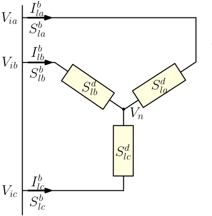
(a) Wye connection

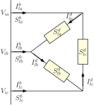
(b) Delta connection

Figure 3: Three-phase load configuration

Figure 3(a) illustrates a three-phase wye-connected load $l\in\mathcal{Y}$ at bus $i\in\mathcal{N}$. Note that for each $\phi\in\mathcal{P}$, the voltage applied to the load (i.e., $V_{l\phi}$) is $V_{i\phi}$ and the current passing through the load (i.e., $I^{d}_{l\phi}$) is $I_{l\phi}^{b}$ and thus

$$\boldsymbol{S}^{b}_{l}=\boldsymbol{S}^{d}_{l}.$$ (10)

For a three-phase delta-connected load $l\in\mathcal{D}$ at bus $i\in\mathcal{N}$, as illustrated in Figure 3(b), the voltage applied to the load is

$$\boldsymbol{V}_{l}={\boldsymbol{\Lambda}}\boldsymbol{V}_{i},$$ (11)

where

$${\boldsymbol{\Lambda}}=\left[\begin{array}[]{ccc}1&-1&0\\ 0&1&-1\\ -1&0&1\end{array}\right].$$

In addition, from Kirchhoff’s current law, we have

$$\boldsymbol{I}^{b}_{l}={\boldsymbol{\Lambda}}^{\top}\boldsymbol{I}_{l}^{d}.$$ (12)

Therefore,

$$\boldsymbol{S}^{d}_{l}=\mbox{diag}(\boldsymbol{V}_{l}(\boldsymbol{I}_{l}^{d})^{H})=\mbox{diag}({\boldsymbol{\Lambda}}\boldsymbol{V}_{i}(\boldsymbol{I}_{l}^{d})^{H}),$$ (13a)

$$\boldsymbol{S}^{b}_{l}=\mbox{diag}(\boldsymbol{V}_{i}(\boldsymbol{I}^{b}_{l})^{H})=\mbox{diag}(\boldsymbol{V}_{i}(\boldsymbol{I}^{d}_{l})^{H}{\boldsymbol{\Lambda}}).$$ (13b)

By replacing each $\boldsymbol{I}^{b}_{l}$ with $\boldsymbol{I}^{d}_{l}$ for $l\in\mathcal{Y}$ and with ${\boldsymbol{\Lambda}}^{\top}\boldsymbol{I}^{d}_{l}$ for $l\in\mathcal{D}$ in the physical laws and introducing auxiliary variables $\boldsymbol{L}^{d}_{eij}$ for $\boldsymbol{I}^{d}_{l}(\boldsymbol{I}^{d}_{l})^{H}$ and $\boldsymbol{X}_{l}$ for $\boldsymbol{V}_{i}(\boldsymbol{I}^{d}_{l})^{H}$, we can derive the AC OPF problem with delta connections as follows:
(AC-D):

$$\min\ \sum_{k\in\mathcal{G}}C_{k}(\boldsymbol{S}^{g}_{k})$$

s.t. $$\eqref{eq:acpf:rank1}-\eqref{eq:acpf:power-loss},\eqref{eq:acpf:power-bal},\eqref{eqs:op-constr},$$ (14a)

$$\forall l\in\mathcal{L}:$$

$$\quad\quad\boldsymbol{S}_{l}^{d}={\color[rgb]{0,0,0}\boldsymbol{S}^{0}_{l}},$$ (14b)

$$\forall i\in\mathcal{N},l\in\mathcal{D}(i):$$

$$\quad\quad\left[\begin{array}[]{cc}\boldsymbol{W}_{i}&\boldsymbol{X}_{l}\\ \boldsymbol{X}_{l}^{H}&\boldsymbol{L}^{d}_{l}\end{array}\right]=\left[\begin{array}[]{c}\boldsymbol{V}_{i}\\ \boldsymbol{I}^{d}_{l}\end{array}\right]\left[\begin{array}[]{c}\boldsymbol{V}_{i}\\ \boldsymbol{I}^{d}_{l}\end{array}\right]^{H},$$ (14i)

$$\quad\quad\boldsymbol{S}_{l}^{d}=\mbox{diag}(\boldsymbol{\Lambda}\boldsymbol{X}_{l}),$$ (14j)

$$\quad\quad\boldsymbol{S}_{l}^{b}=\mbox{diag}(\boldsymbol{X}_{l}\boldsymbol{\Lambda}),$$ (14k)

$$\quad\quad I^{d}_{l\phi}=0,\ \forall\phi\notin\mathcal{P}_{l},$$ (14l)

$$\forall i\in\mathcal{N},l\in\mathcal{Y}(i):\eqref{eq:wye:power}.$$ (14m)

III-A1 SDP relaxation of (AC-D)

In [8], a SDP relaxation of (AC-D) is proposed, which builds on (SD) and further relaxes the rank-1 requirement of Equation (14i):

$$\mbox{(SDP-D)}:\min\ \sum_{k\in\mathcal{G}}C_{k}(\boldsymbol{S}^{g}_{k})$$

s.t. $$\eqref{eq:opf:sdp},\eqref{eq:acpf:power-eq},\eqref{eq:acpf:power-loss},\eqref{eq:acpf:power-bal},\mbox{ and }\eqref{eqs:op-constr},$$ (15a)

$$\forall i\in\mathcal{N},l\in\mathcal{D}(i):$$

$$\quad\quad\left[\begin{array}[]{cc}\boldsymbol{W}_{i}&\boldsymbol{X}_{l}\\ \boldsymbol{X}_{l}^{H}&\boldsymbol{L}^{d}_{l}\end{array}\right]\succeq 0,$$ (15d)

$$\quad\quad\boldsymbol{L}^{d}_{l\phi\cdot}=0,\ \forall\phi\notin\mathcal{P}_{e},$$ (15e)

$$\eqref{eq:acpf-d:load-power},\eqref{eq:acpf-d:delta:power-connection1},\eqref{eq:acpf-d:delta:power-connection2},\eqref{eq:acpf-d:wye:power-connection},$$ (15f)

where $\boldsymbol{L}^{d}_{l\phi\cdot}$ denote the row of $\boldsymbol{L}^{d}_{l}$ corresponding to $\phi$.

Remark 1.

In [9], the authors show that (SDP-D) is often inexact because of the nonuniqueness of $\boldsymbol{L}_{l}^{d}$ and a spectrum error in computation. The authors proposed an algorithm that can produce an exact solution of (SDP-D) when a sufficient condition holds. The algorithm imposes a penalty on the trace of $\boldsymbol{L}_{l}^{d}$ in the objective function of (SDP-D), namely, $\rho\sum_{l\in\mathcal{D}}\mbox{tr}(\boldsymbol{L}_{l}^{d})$ with some penalty weight $\rho>0$. If the modified problem produces a rank-1 solution, it is globally optimal to (AC-D).

III-A2 Linear approximation of (AC-D)

We propose a linear approximation of Equation (13) that can be readily added to (LP) under Assumption 1. Note that by taking the conjugate transpose of each side of Equation (12) and multiplying both sides with $\boldsymbol{V}_{i}$ from the left, we have $\sum_{\phi\in\mathcal{P}}S^{b}_{l\phi}=\sum_{\phi\in\mathcal{P}}{S^{d}_{l\phi}}$. In addition, by Assumption 1 (b), it follows that

$${S_{la}^{d}}=(V_{ia}-\gamma V_{ia})(I^{d}_{la})^{H}\Longrightarrow V_{ia}(I^{d}_{la})^{H}=\frac{1}{1-\gamma}{S_{la}^{d}},$$ (16)

where $\gamma=e^{-\mathrm{i}(2\pi/3)}=-\frac{1}{2}-\mathrm{i}\frac{\sqrt{3}}{2}$. Using Equation (16) and Assumption 1 (b), we can express $S^{d}_{lb}$ and $S^{d}_{lc}$ as follows:

$${S_{lb}^{d}} =(\gamma V_{ia}-\gamma^{2}V_{ia})(I_{lb}^{d})^{H}=(1-\gamma)\gamma V_{ia}(I_{lb}^{b}+I_{la}^{d})^{H}$$

$$=(1-\gamma)\gamma\left[\frac{1}{\gamma}S^{b}_{lb}+\frac{1}{1-\gamma}{S^{d}_{la}}\right],$$

$${S_{lc}^{d}} =(\gamma^{2}V_{ia}-V_{ia})(I_{lc}^{d})^{H}=(\gamma^{2}-1)V_{ia}(I_{lb}^{b}+I_{lc}^{b}+I_{la}^{d})^{H}$$

$$=(\gamma^{2}-1)\left[\frac{1}{\gamma}S^{b}_{lb}+\frac{1}{\gamma^{2}}S^{b}_{lc}+\frac{1}{1-\gamma}{S^{d}_{la}}\right].$$

By expressing the equations in real and imaginary parts, we derive the following linear system of equations that connect $\boldsymbol{S}^{d}_{l}$ and $\boldsymbol{S}^{b}_{l}$ for each delta load $l\in\mathcal{D}$:

$$p_{l1}^{b}+p_{l2}^{b}+p_{l3}^{b}={p_{l1}^{d}+p_{l2}^{d}+p_{l3}^{d}},$$ (17a)

$$q_{l1}^{b}+q_{l2}^{b}+q_{l3}^{b}={q_{l1}^{d}+q_{l2}^{d}+q_{l3}^{d}},$$ (17b)

$$\frac{3}{2}p^{b}_{l2}-\frac{\sqrt{3}}{2}q^{b}_{l2}={p^{d}_{l2}+\frac{1}{2}p^{d}_{l1}-\frac{\sqrt{3}}{2}q^{d}_{l1}},$$ (17c)

$$\frac{\sqrt{3}}{2}p^{b}_{l2}+\frac{3}{2}q^{b}_{l2}={\frac{\sqrt{3}}{2}p^{d}_{l1}+\frac{1}{2}q^{d}_{l1}+q^{d}_{l2}},$$ (17d)

$$\sqrt{3}q^{b}_{l2}+\frac{3}{2}p^{b}_{l3}-\frac{\sqrt{3}}{2}q^{b}_{l3}={\frac{1}{2}p^{d}_{l1}+\frac{\sqrt{3}}{2}q^{d}_{l1}+p^{d}_{l3}},$$ (17e)

$$-\sqrt{3}p^{b}_{l2}+\frac{\sqrt{3}}{2}p^{b}_{l3}+\frac{3}{2}q^{b}_{l3}={-\frac{\sqrt{3}}{2}p^{d}_{l1}+\frac{1}{2}q^{d}_{l1}+q^{d}_{l3}}.$$ (17f)

Remark 2.

Note that Equation (17) is a system of 6 linear equations with 6 unknowns, say, $A\boldsymbol{x}=b$. Since the corresponding square matrix $A\in\mathbb{R}^{6\times 6}$ is invertible, $\boldsymbol{p}^{b}_{l}$ and $\boldsymbol{q}^{b}_{l}$ are uniquely defined once $\boldsymbol{p}^{d}_{l}$ and $\boldsymbol{q}^{d}_{l}$ are determined. This implies that under Assumption 1, Equation (17) exactly describes the relationship between $\boldsymbol{S}^{b}$ and $\boldsymbol{S}^{d}$ for delta-connected devices.

To summarize, the linear approximation of (AC-D) can be expressed as follows:

$$\mbox{(LP-D)}:\min\ \sum_{k\in\mathcal{G}}C_{k}(\boldsymbol{S}^{g}_{k})$$

s.t. $$\eqref{eqs:acopf:lp},\eqref{eq:acpf-d:load-power},$$ (18a)

$$\forall l\in\mathcal{D}:\eqref{eq:delta:power},$$ (18b)

$$\forall l\in\mathcal{Y}:\eqref{eq:wye:power}.$$ (18c)

Remark 3.

Note that the linear approximation of the delta connection (i.e., Equation (17)) can also be applied to any delta-connected network components (e.g., generators in delta connections). It approximates the bus injection/withdrawal $\boldsymbol{S}^{b}$ of a delta-connected device based on its power production/consumption $\boldsymbol{S}^{d}$.

III-B Exponential load model

In the preceding sections we assumed that the power consumption of load $l\in\mathcal{L}$ at phase $\phi$ (i.e., $S^{d}_{l\phi}$) is constant at its nominal power $\color[rgb]{0,0,0}S^{0}_{l\phi}=p^{0}_{l\phi}+\mathrm{i}q^{0}_{l\phi}$. In practice, however, $\boldsymbol{S}^{d}_{l}$ changes depending on the applied voltage. A widely used model for voltage-dependent load is an exponential load model that assumes that the power consumption of a load is proportional to the applied voltage magnitude raised to some power [13]. For each multiphase load $l\in\mathcal{L}$, its power consumption at phase $\phi\in\mathcal{P}$, namely., $S^{d}_{l\phi}=p^{d}_{l\phi}+\mathbf{i}q^{d}_{l\phi}$, is computed by

$$p^{d}_{l\phi}={\color[rgb]{0,0,0}p^{0}_{l\phi}}\left(\frac{|V_{l\phi}|}{{|\color[rgb]{0,0,0}V^{0}_{l\phi}|}}\right)^{{\color[rgb]{0,0,0}\alpha_{l\phi}}},\ \ q^{d}_{l\phi}={\color[rgb]{0,0,0}q^{0}_{l\phi}}\left(\frac{|V_{l\phi}|}{{|\color[rgb]{0,0,0}V^{0}_{l\phi}|}}\right)^{{\color[rgb]{0,0,0}\beta_{l\phi}}},$$ (19)

where $p^{d}_{l\phi}$ (resp., $q^{d}_{l\phi}$) denotes the active (resp., reactive) power consumption of $l$ at phase $\phi$ when the magnitude of voltage applied to the load is $|V_{l\phi}|$ and where ${\color[rgb]{0,0,0}p^{0}_{l\phi}}$, ${\color[rgb]{0,0,0}q^{0}_{l\phi}}$, and ${|\color[rgb]{0,0,0}V^{0}_{l\phi}|}$ respectively denote reference values for active power load, reactive power load, and voltage magnitude applied to the load, which are given as data. The exponents ${\color[rgb]{0,0,0}\alpha_{l\phi}}$ and ${\color[rgb]{0,0,0}\beta_{l\phi}}$ are also given as data, which are nonnegative numbers that characterize the voltage dependency of load $l$. For instance, some special choice of the exponents yields classical load models; With the exponents ${\color[rgb]{0,0,0}\alpha_{l\phi}}$ and ${\color[rgb]{0,0,0}\beta_{l\phi}}$ equal to $0$, $1$, and $2$, Equation (19) represents constant power, constant current, and constant impedance load, respectively. Exponent values other than 0, 1, or 2 can be employed to model more general load types; see, for example, [13].

We denote the coefficients of Equation (19) by $\color[rgb]{0,0,0}a_{l\phi}$ and $\color[rgb]{0,0,0}b_{l\phi}$ (i.e., $\color[rgb]{0,0,0}a_{l\phi}=\frac{p_{l\phi}^{0}}{|V^{0}_{l\phi}|^{\alpha_{l\phi}}}$ and $\color[rgb]{0,0,0}b_{l\phi}=\frac{q_{l\phi}^{0}}{|V^{0}_{l\phi}|^{\beta_{l\phi}}}$). Without loss of generality, we assume that $\color[rgb]{0,0,0}a_{l\phi}$ and $\color[rgb]{0,0,0}b_{l\phi}$ are nonzeros, since otherwise the corresponding values of $p^{d}_{l\phi}$ and $q^{d}_{l\phi}$ become trivial as zeros. Now we may express Equation (19) in terms of the squared magnitude of voltage applied to load $l$ at phase $\phi$, denoted by $v_{l\phi}=|V_{l\phi}|^{2}$:

$$\frac{1}{{\color[rgb]{0,0,0}a_{l\phi}}}p^{d}_{l\phi}=v_{l\phi}^{\frac{\color[rgb]{0,0,0}\alpha_{l\phi}}{2}},\ \ \frac{1}{{\color[rgb]{0,0,0}b_{l\phi}}}q^{d}_{l\phi}=v_{l\phi}^{\frac{\color[rgb]{0,0,0}\beta_{l\phi}}{2}},$$ (20)

where

$$\boldsymbol{v}_{l}=\mbox{diag}(\boldsymbol{V}_{i}\boldsymbol{V}_{i}^{H})=\mbox{diag}(\boldsymbol{W}_{i}),\ \forall l\in\mathcal{Y}(i),$$ (21a)

$$\boldsymbol{v}_{l}=\mbox{diag}(\boldsymbol{\Lambda}\boldsymbol{V}_{i}(\boldsymbol{\Lambda}\boldsymbol{V}_{i})^{H})=\mbox{diag}(\boldsymbol{\Lambda}\boldsymbol{W}_{i}\boldsymbol{\Lambda}^{\top}),\ \forall l\in\mathcal{D}(i).$$ (21b)

To summarize, AC OPF with delta-connected exponential loads can be posed as follows:

$$\mbox{(AC-D-E)}:\min\ \sum_{k\in\mathcal{G}}C_{k}(\boldsymbol{S}^{g}_{k})$$

s.t. $$\eqref{eq:acpf-d:acpf},\eqref{eq:acpf-d:rank1}-\eqref{eq:acpf-d:wye:power-connection},\eqref{volt-dependent-model-2},\eqref{eqs:exp-load:volt}.$$

III-B1 Convex relaxation of exponential load model

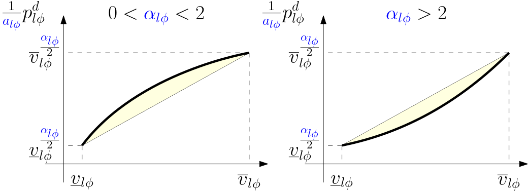
Figure 4: Graphical illustration of the convex relaxation of Equation (20) for $\alpha_{l\phi}\neq 0,2$ (i.e., (23a)–(23d))

In [12] the authors proposed a convex relaxation of Equation (20) that can be readily added to (SDP-D). Note that $\frac{1}{{\color[rgb]{0,0,0}a_{l\phi}}}p^{d}_{l\phi}$ (or $\frac{1}{{\color[rgb]{0,0,0}b_{l\phi}}}q^{d}_{l\phi}$) is always positive independently of the sign of $\color[rgb]{0,0,0}a_{l\phi}$ (or $\color[rgb]{0,0,0}b_{l\phi}$). If ${\color[rgb]{0,0,0}\alpha_{l\phi}}$ (or $\color[rgb]{0,0,0}\beta_{l\phi}$) is either to 0 or 2, Equation (20) yields the following linear constraints:

$$p^{d}_{l\phi}={\color[rgb]{0,0,0}p^{0}_{l\phi}},\ \forall l,\phi\mbox{ with }\alpha_{l\phi}=0,$$ (22a)

$$p^{d}_{l\phi}={\color[rgb]{0,0,0}a_{l\phi}}v_{l\phi},\ \forall l,\phi\mbox{ with }\alpha_{l\phi}=2.$$ (22b)

Otherwise, that is, if ${\color[rgb]{0,0,0}\alpha_{l\phi}}$ (or $\color[rgb]{0,0,0}\beta_{l\phi}$) is not equal to 0 or 2, Equation (20) becomes either a strictly convex curve for $\color[rgb]{0,0,0}\alpha_{l\phi}$ (or $\color[rgb]{0,0,0}\beta_{l\phi}$) $>2$ or a strictly concave curve for $0<\color[rgb]{0,0,0}\alpha_{l\phi}$ (or $\color[rgb]{0,0,0}\beta_{l\phi}$) $<2$. Therefore, the nonlinear curves can be relaxed with their convex epigraphs or hypographs. In addition, the relaxation can be made tighter by adding valid affine over- or underestimators, using bounds on the magnitude of applied voltage on loads (i.e., say, $\color[rgb]{0,0,0}\underline{\boldsymbol{v}}_{l},\overline{\boldsymbol{v}}_{l}$), if available. Figure 4 illustrates the corresponding convex relaxation of Equation (20), which can be expressed as follows:

$$\frac{1}{\color[rgb]{0,0,0}a_{l\phi}}p^{d}_{l\phi}\geq\ell(v_{l\phi}),\ \forall l,\phi\mbox{ with }0<\alpha_{l\phi}<2,$$ (23a)

$$\frac{1}{\color[rgb]{0,0,0}a_{l\phi}}p^{d}_{l\phi}\leq\ell(v_{l\phi}),\ \forall l,\phi\mbox{ with }\alpha_{l\phi}>2,$$ (23b)

$$\frac{1}{\color[rgb]{0,0,0}a_{l\phi}}p^{d}_{l\phi}\leq v_{l\phi}^{\frac{\color[rgb]{0,0,0}\alpha_{l\phi}}{2}},\ \forall l,\phi\mbox{ with }0<\alpha_{l\phi}<2,$$ (23c)

$$\frac{1}{{\color[rgb]{0,0,0}a_{l\phi}}}p^{d}_{l\phi}\geq v_{l\phi}^{\frac{\color[rgb]{0,0,0}\alpha_{l\phi}}{2}},\ \forall l,\phi\mbox{ with }\alpha_{l\phi}>2,$$ (23d)

where $\ell(v_{l\phi})=\frac{\color[rgb]{0,0,0}\overline{v}_{l\phi}^{\frac{\color[rgb]{0,0,0}\alpha_{l\phi}}{2}}-\underline{v}_{l\phi}^{\frac{\color[rgb]{0,0,0}\alpha_{l\phi}}{2}}}{\color[rgb]{0,0,0}\overline{v}_{l\phi}-\underline{v}_{l\phi}}(v_{l\phi}-{\color[rgb]{0,0,0}\underline{v}_{l\phi}})+{\color[rgb]{0,0,0}\underline{v}_{l\phi}^{\frac{\alpha_{l\phi}}{2}}}$. The authors in [12] also remarked that Equations (23c) and (23d) can be respectively expressed as equivalent power cone constraints:

$$(v_{l\phi},1,p^{d}_{l\phi}/{\color[rgb]{0,0,0}a_{l\phi}})\in\mathbb{P}_{3}({\color[rgb]{0,0,0}\alpha_{l\phi}}/2),$$ (24a)

$$(p^{d}_{l\phi}/{\color[rgb]{0,0,0}a_{l\phi}},1,v_{l\phi})\in\mathbb{P}_{3}(2/{\color[rgb]{0,0,0}\alpha_{l\phi}}),$$ (24b)

where $\mathbb{P}_{3}(e):=\{\boldsymbol{x}\in\mathbb{R}^{3}:x_{1}^{e}x_{2}^{1-e}\geq|x_{3}|,x_{1},x_{2}\geq 0\}$. A similar procedure can be applied for the reactive power constraint.

To summarize, the convex relaxation of (AC-D) with exponential loads can be posed as follows:

$$\mbox{(CONVEX-D-E)}:$$

$$\min\ \sum_{k\in\mathcal{G}}C_{k}(\boldsymbol{S}^{g}_{k})$$

s.t. $$\eqref{eq:acopf-d:sdp}-\eqref{eq:acopf-d:sdp:current-on-missing-phase},\eqref{eq:acpf-d:delta:power-connection1},\eqref{eq:acpf-d:delta:power-connection2},\eqref{eq:acpf-d:wye:power-connection},$$

$$\eqref{eqs:exp-load:volt},\eqref{eq:load:sdp:linear},\eqref{eq:load:sdp:concave:affine},\eqref{eq:load:sdp:convex:affine},\eqref{eqs:load:sdp:power-cone}.$$

III-B2 Linear approximation of exponential load model

We utilize the linear approximation of Equation (20) at $v_{l\phi}=1$:

$$p^{d}_{l\phi}=\frac{\color[rgb]{0,0,0}a_{l\phi}\alpha_{l\phi}}{2}(v_{l\phi}-1)+{\color[rgb]{0,0,0}a_{l\phi}},$$ (25a)

$$q^{d}_{l\phi}=\frac{\color[rgb]{0,0,0}b_{l\phi}\beta_{l\phi}}{2}(v_{l\phi}-1)+{\color[rgb]{0,0,0}b_{l\phi}}.$$ (25b)

Note that when the exponents are 0 or 2, the linearized equation correctly represents the constant power and constant impedance load models, respectively.

For delta-connected loads, the voltage applied to the load is $V_{i\phi}-V_{i\phi^{+}}$ for each $\phi\in\mathcal{P}$, and thus $v_{l\phi}=|V_{i\phi}-V_{i\phi^{+}}|^{2}$. Using the assumption that voltages are almost balanced (i.e., Assumption 1 (b)), we approximate $V_{i\phi+}$ with $\gamma V_{i\phi}$, and thus

$$v_{l\phi}=|1-\gamma|^{2}W_{i\phi\phi}=3W_{i\phi\phi}.$$ (26)

In summary, the linear approximation of (AC-D) with exponential loads can be expressed as follows:

$$\mbox{(LP-D-E)}:\min\ \sum_{k\in\mathcal{G}}C_{k}(\boldsymbol{S}^{g}_{k})$$

s.t. $$\eqref{eqs:acopf:lp},\eqref{eq:acopf-d:lp:delta},\eqref{eq:acopf-d:lp:wye},\eqref{eq:volt-dependent-model-linearized},\eqref{eq:exp-load:volt:wye},\eqref{eq:linear:delta:volt}.$$

Remark 4.

Note that if all shunt elements (i.e., ${\color[rgb]{0,0,0}\boldsymbol{Y}_{eij}^{sh}}$ and ${\color[rgb]{0,0,0}\boldsymbol{Y}_{s}^{sh}}$) have zero off-diagonal elements, then the off-diagonal elements of $\boldsymbol{W}_{i}$ become redundant. It is trivial for Equation (1n); for Equation (7a), the radial structure of the network justifies it. Note that once we obtain a solution to a problem in which the off-diagonal elements of $\boldsymbol{W}$ are ignored (see Problem (27)), we can construct the off-diagonal elements of $\boldsymbol{W}$ by first computing $\boldsymbol{W}_{0}$ according to (2c) and then computing $\boldsymbol{W}_{i}$ for the subsequent buses by recursively applying (7a). Note that the resultant $\boldsymbol{W}$ is feasible to (LP-D-E), since the off-diagonal elements do not appear in any other constraints than (7a).

From Remark 4, when all shunt elements have zero off-diagonal elements, (LP-D-E) can be simplified by ignoring terms related to the off-diagonal elements of $\boldsymbol{W}_{i}$ and denoting the diagonal elements of $\boldsymbol{W}_{i}$ (i.e., $|\boldsymbol{V}_{i}|^{2}$) as $\boldsymbol{v}_{i}$:

$$\min\ \sum_{k\in\mathcal{G}}C_{k}(\boldsymbol{S}^{g}_{k})$$

s.t. $$\forall(e,i,j)\in\mathcal{E}:$$

$$\quad\boldsymbol{v}_{j}=\boldsymbol{v}_{i}-\mbox{diag}(\boldsymbol{M}_{eij}{\color[rgb]{0,0,0}\boldsymbol{Z}_{e}^{H}}+{\color[rgb]{0,0,0}\boldsymbol{Z}_{e}}\boldsymbol{M}_{eij}^{H}),$$ (27a)

$$\quad\boldsymbol{S}_{eji}=-\boldsymbol{S}_{eij},$$ (27b)

$$\quad\boldsymbol{M}_{eij}=\boldsymbol{\Gamma}\mbox{diag}(\boldsymbol{S}_{eij}),$$ (27c)

$$\forall i\in\mathcal{N}:$$

$$\quad\sum_{(e,i,j)\mbox{ or }(e,j,i)\in\mathcal{E}}\boldsymbol{S}_{eij}+({\color[rgb]{0,0,0}\boldsymbol{Y}^{sh}_{eij}})^{H}\boldsymbol{v}_{i}=$$

$$\quad\sum_{s\in\mathcal{B}(i)}({\color[rgb]{0,0,0}\boldsymbol{Y}^{sh}_{s}})^{H}\boldsymbol{v}_{i}+\sum_{k\in\mathcal{G}(i)}\boldsymbol{S}^{g}_{k}-\sum_{l\in\mathcal{L}(i)}{\color[rgb]{0,0,0}\boldsymbol{S}^{b}_{l}},$$ (27d)

$$\quad{\color[rgb]{0,0,0}\underline{v}_{i\phi}^{2}}\leq v_{i\phi}\leq{\color[rgb]{0,0,0}\overline{v}_{i\phi}^{2}},\ \forall\phi\in\mathcal{P},$$ (27e)

$$\quad\boldsymbol{v}_{l}=\boldsymbol{v}_{i},\ \forall l\in\mathcal{Y}(i),$$ (27f)

$$\quad\boldsymbol{v}_{l}=3\boldsymbol{v}_{i},\ \forall l\in\mathcal{D}(i),$$ (27g)

$$\forall l\in\mathcal{L}:$$ (27h)

$$\quad p^{d}_{l\phi}=\frac{\color[rgb]{0,0,0}a_{l\phi}\alpha_{l\phi}}{2}(v_{l\phi}-1)+{\color[rgb]{0,0,0}a_{l\phi}},$$ (27i)

$$\quad q^{d}_{l\phi}=\frac{\color[rgb]{0,0,0}b_{l\phi}\beta_{l\phi}}{2}(v_{l\phi}-1)+{\color[rgb]{0,0,0}b_{l\phi}},$$ (27j)

$$\boldsymbol{S}^{g}_{k}\in\mathcal{S}_{k},\ \forall k\in\mathcal{G},$$ (27k)

$$v_{0\phi}=|V_{0\phi}^{ref}|^{2},\ \forall\phi\in\mathcal{P}_{0},$$ (27l)

$$\eqref{eq:acopf-d:lp:delta},\eqref{eq:acopf-d:lp:wye}.$$ (27m)

IV Numerical results

In this section we analyze the performance of the proposed linear approximation of (AC-D-E) on the IEEE 13, 37, and 123 bus systems. The generation cost function $C_{k}(\boldsymbol{S}_{k}^{g})$ for each $k\in\mathcal{G}$ is defined to be the sum of its real power generation $\sum_{\phi\in\mathcal{P}_{k}}p_{k\phi}$. In these test systems, only the voltage source serves as a generator, and thus the problem minimizes the total import from the transmission grid. The voltage bounds are set to be [0.8 p.u., 1.2 p.u.]. Substation transformers and regulators are removed, and the load transformers are modeled as lines with equivalent impedance. We eliminate switches or regard them as lines according to their default status. All capacitors are assumed active and generate reactive power according to their ratings and the associated bus voltages. Substations voltages are set as $V_{0}^{ref}=\bar{V}[1,e^{-j2\pi/3},e^{j2\pi/3}]^{T}$, where $\bar{V}$ is given as the substation voltage in the test systems. This experiment setup is commonly used in the literature [8, 9]. For the experiments of (SDP-D) and (CONVEX-D-E), we set the penalty weight $\rho$ for minimizing the rank of $\boldsymbol{L}_{l}^{d}$ (see Remark 1) to be 100. Once (SDP-D) and (CONVEX-D-E) are solved, the resultant penalty term is subtracted from the objective value to calculate the true objective value.

All experiments were executed on a Mac machine with 32 GB of memory on an Intel Core i7 at 2.3 GHz. The nonconvex AC formulations were solved by using Ipopt 3.14.4, running with linear solver MUMPS 5.4.1, the convex conic formulations were by Mosek 9.3, and the linear models were via CPLEX 20.1.

IV-A Performance of (SDP-D) and (LP-D)

TABLE I: Maximum ratio between the top two largest eigenvalues of PSD matrices in (SDP-D)

Instance	$\max_{i\in\mathcal{N}^{leaf}}\lambda(\boldsymbol{W}_{i})$	$\max_{e\in\mathcal{E}}\lambda(\boldsymbol{B}_{e})$	$\max_{l\in\mathcal{D}}\lambda(\boldsymbol{C}_{l})$
IEEE 13	$6.10\times 10^{-9}$	$7.23\times 10^{-7}$	$3.79\times 10^{-8}$
IEEE 37	$1.01\times 10^{-8}$	$3.22\times 10^{-8}$	$2.13\times 10^{-8}$
IEEE 123	$8.12\times 10^{-9}$	$2.25\times 10^{-8}$	$1.06\times 10^{-8}$

To see the performance of the linearized model for the delta connection, we first compare (AC-D), (SDP-D), and (LP-D) by fixing all loads at their nominal power (i.e., the constant power model). As noted in [9], we observe that (SDP-D) produces rank-1 solutions for all the test systems. Table I displays the maximum ratio between the top two largest eigenvalues of $\boldsymbol{W}_{i}$ for $i\in\mathcal{N}^{leaf}$, $\boldsymbol{B}_{e}:=\left[\begin{array}[]{cc}\boldsymbol{W}_{i}&\boldsymbol{M}_{eij}\\ \boldsymbol{M}^{H}_{eij}&\boldsymbol{L}_{eij}\end{array}\right]$ for $(e,i,j)\in\mathcal{E}$, and $\boldsymbol{C}_{l}:=\left[\begin{array}[]{cc}\boldsymbol{W}_{i}&\boldsymbol{X}_{l}\\ \boldsymbol{X}_{l}^{H}&\boldsymbol{L}^{d}_{l}\end{array}\right]$ for $l\in\mathcal{D}$ returned by the solvers, where $\lambda(A)$ denotes the ratio between the two largest eigenvalues of a matrix $A$. The result suggests that all the PSD matrices are almost rank-1, implying the global optimality of the (SDP-D) solutions. Surprisingly, we observe that (AC-D) also produces a globally optimal solution that complies with (SDP-D), providing the same objective values, $\boldsymbol{w}$, and $\boldsymbol{S}^{b}$ as (SDP-D) for all the test instances.

TABLE II: Performance of (LP-D) with respect to (SDP-D)

Instance	LP-D
	$\Delta\boldsymbol{w}(\%)$	$\Delta\boldsymbol{p}^{b}(\%)$	$\Delta\boldsymbol{q}^{b}(\%)$
IEEE 13	0.93	0.55	3.32
IEEE 37	0.12	0.5	2.1
IEEE 123	0.41	0.07	0.59

TABLE III: Solution time in seconds

Instance	AC-D	SDP-D	LP-D
IEEE 13	2.31	0.92	0.003
IEEE 37	3.51	2.50	0.006
IEEE 123	4.74	6.55	0.059

Table II compares the solutions of (LP-D) with those of (SDP-D) to see the performance of the linearization, where $\Delta\boldsymbol{x}$ represents the average relative difference in variable $\boldsymbol{x}$; that is, $\Delta\boldsymbol{x}=\sum_{i=1}^{n}\frac{|x_{i}^{LP}-x_{i}^{SDP}|}{|x_{i}^{SDP}|}/n$, where $n$ denotes the dimension of $\boldsymbol{x}$. The result suggests that the error does not exceed 1% for the voltage magnitudes and the real power withdrawals for all the instances. In addition, as shown in Table III, the computation time of (LP-D) is faster than that of (SDP-D) by at least two orders of magnitude.

IV-B Performance of (CONVEX-D-E) and (LP-D-E)

TABLE IV: Maximum ratio between the top two largest eigenvalues of PSD matrices in (CONVEX-D-E)

Instance	$\max_{i\in\mathcal{N}^{leaf}}\lambda(\boldsymbol{W}_{i})$	$\max_{e\in\mathcal{E}}\lambda(\boldsymbol{B}_{e})$	$\max_{l\in\mathcal{D}}\lambda(\boldsymbol{C}_{l})$
IEEE 13	$2.16\times 10^{-10}$	$4.79\times 10^{-8}$	$6.38\times 10^{-10}$
IEEE 37	$3.22\times 10^{-11}$	$9.56\times 10^{-11}$	$6.26\times 10^{-11}$
IEEE 123	$1.17\times 10^{-10}$	$3.54\times 10^{-10}$	$1.24\times 10^{-10}$

TABLE V: Objective value comparison

Instance	AC-D-E	CONVEX-D-E	LP-D-E
IEEE 13	3175.31	3134.30	3093.96
IEEE 37	2027.85	1933.56	2029.88
IEEE 123	2533.46	2476.47	2504.57

TABLE VI: Relative difference in percentage from solutions of (AC-D-E)

Instance	CONVEX-D-E			LP-D-E
	$\Delta\boldsymbol{w}$	$\Delta\boldsymbol{p}^{b}$	$\Delta\boldsymbol{q}^{b}$	$\Delta\boldsymbol{w}$	$\Delta\boldsymbol{p}^{b}$	$\Delta\boldsymbol{q}^{b}$
IEEE 13	0.26	1.49	1.76	0.6	0.7	3.96
IEEE 37	0.2	5.44	7.26	0.04	2.96	5.07
IEEE 123	0.1	0.9	1.41	0.16	0.36	0.58

TABLE VII: Solution time in seconds

Instance	AC-D-E	CONVEX-D-E	LP-D-E
IEEE 13	2.38	1.60	0.004
IEEE 37	2.93	2.98	0.007
IEEE 123	5.61	5.98	0.078

In this section we analyze the performance of the formulations with exponential load models. Table IV displays the maximum ratio between the two largest eigenvalues of $\boldsymbol{W}_{i}$ for $i\in\mathcal{N}^{leaf}$, $\boldsymbol{B}_{e}$ for $(e,i,j)\in\mathcal{E}$, and $\boldsymbol{C}_{l}$ for $l\in\mathcal{D}$ returned as a solution to (CONVEX-D-E) by the solvers. Although the solver returns rank-1 solutions for all the instances, (CONVEX-D-E) no longer provides globally optimal solutions to (AC-D-E) but can serve as a lower bound since the conic reformulation of the exponential load model is not exact unless all loads have $\alpha=0\mbox{ or }2$ and $\beta=0\mbox{ or }2$. Since all the test cases include loads with exponents that are not 0 or 2, (CONVEX-D-E) provides strict lower bounds, as shown in Table V. Table VI summarizes the average relative differences between solutions of (AC-D-E) and those of (CONVEX-D-E) and (LP-D-E). The relative difference between the LP solution and a feasible AC solution does not exceed 1% with regard to the voltage magnitudes and 3% for the real power withdrawals. In addition, as shown in Table VII, (LP-D-E) yields solutions faster than (CONVEX-D-E) does by at least two orders of magnitude.

IV-C Importance of modeling delta-connected, voltage-dependent loads

In this section we demonstrate the importance of incorporating delta connections and voltage-dependent loads into OPF. In this simulation, the IEEE 37-bus distribution feeder is utilized since all of its loads are configured as delta. All loads are assumed to be exponential loads, and the experiments are done by uniformly varying the exponents of all the loads (i.e., $\alpha_{l,\phi},\beta_{l,\phi}\ \forall l\in\mathcal{L},\phi\in\mathcal{P}_{l}$) from 0 to 3. Thus, it will include cases in which all loads are modeled as constant power ($\alpha_{l,\phi}=\beta_{l,\phi}=0$), constant current ($\alpha_{l,\phi}=\beta_{l,\phi}=1$), and constant impedance ($\alpha_{l,\phi}=\beta_{l,\phi}=2$). In the following subsections, we first show modeling delta-connected, exponential loads since wye configurations can display a contradictory behavior. Subsequently, we demonstrate how different formulations for OPF with delta-connected, voltage-dependent loads behave with varying choices of the exponents, which suggests cases where one formulation outperforms another formulation.

IV-C1 Importance of delta-connection modeling

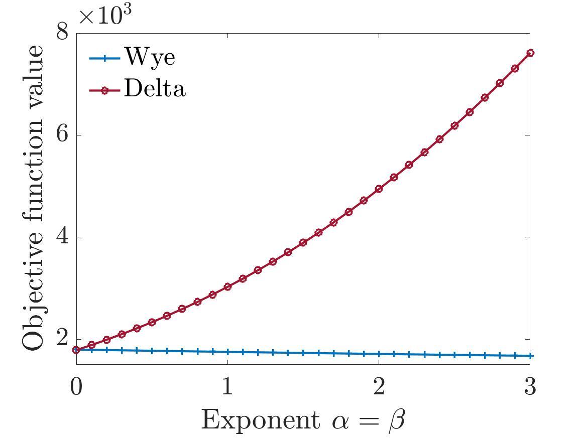
Figure 5: Comparison of (AC-D-E) and (AC-W-E) with varying exponents

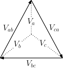
Figure 6: Line-to-line voltage magnitudes

Let (AC-W-E) be the same as (AC-D-E) except that all the loads are assumed to be connected in wye configurations. Figure 5 displays how the objective function value changes as we uniformly increase the exponents. Note that the two models show opposite behaviors: as we increase the exponents, the objective function value of (AC-D-E) increases, but that of (AC-W-E) decreases. The reason is that line-to-line voltage magnitudes are normally larger than line-to-neutral voltage magnitudes (see, e.g., Figure 6). Note that when $v_{l\phi}\leq 1$ p.u., $v_{l\phi}^{\alpha_{l\phi}/2}\geq v_{l\phi}^{\alpha^{\prime}_{l\phi}/2}$ for $0\leq\alpha_{l\phi}\leq\alpha^{\prime}_{l\phi}$. Therefore, if all loads are assumed to be connected in wye configurations, the total power consumption decreases as the exponent increases when the bus voltage magnitudes are under 1 p.u., which is the case of the test system in which the reference voltage magnitude is set as 1 p.u. In fact, however, the applied voltage magnitudes for delta-connected devices are normally above 1 p.u. In this case, the total power consumption increases as we increase the exponent, as shown in Figure 5. The error of the wye modeling gets larger as the exponent grows; note that for the constant power model (i.e., $\alpha=\beta=0$), we have a minor difference in the objective function values, but for the case with $\alpha=\beta=3$, the objective function value is underestimated by almost a factor of 1/4.

IV-C2 Comparison of OPF models with varying exponents

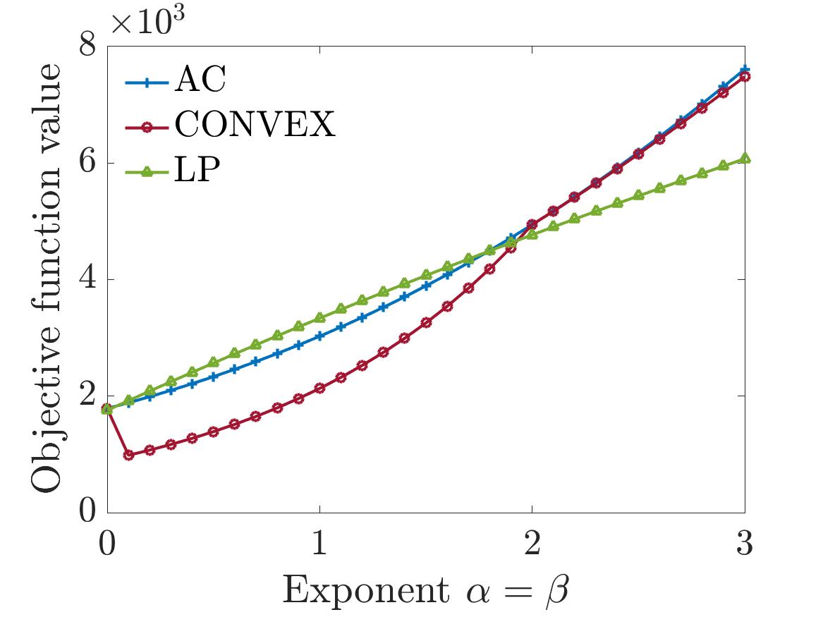
Figure 7: Comparison of (AC-D-E), (CONVEX-D-E), and (LP-D-E) with exponents varied from 0 to 3

Figure 7 plots the objective function values of three different formulations for OPF with delta-connected exponential loads, (AC-D-E), (CONVEX-D-E), and (LP-D-E), according to different choices of the exponent. Note that for $0\leq\alpha=\beta<2$, (LP-D-E) yields objective function values close to (AC-D-E) and that for $\alpha=\beta\geq 2$, (CONVEX-D-E) outperforms (LP-D-E). This behavior is expected from the characteristics of the convex relaxation (i.e., Equation (23)) and the linear approximation (i.e., Equation (25)) of the exponential load model. Note that for $0\leq\alpha=\beta\leq 2$, the linear approximation overestimates the total power consumption, and otherwise it is an underestimation. This explains why (LP-D-E) has a lower objective value for $0\leq\alpha=\beta\leq 2$ and a higher objective value for $\alpha=\beta>2$ than those of (AC-D-E). When $\alpha=\beta=$ 0 or 2 (i.e., when the linearized load model is exact), the objective function value of (LP-D-E) is slightly smaller than that of (AC-D-E) since (LP) ignores power losses. Note also that as the exponent increases above 2, the linear approximation has a larger error when the voltage magnitude deviates from 1 p.u., so the difference between the objective values gets larger. On the other hand, for the convex relaxation (i.e., Equation (23)), since the objective is to minimize the total power generation, $p^{d}_{l\phi}$ is more likely to occur on the underestimator; to be specific, $p^{d}_{l\phi}$ is likely to be chosen on the line $l(v_{l\phi})$ when $0\leq\alpha=\beta\leq 2$ and on the curve $v_{l\phi}^{\alpha_{l\phi}/2}$ for $\alpha=\beta>2$ (see, e.g., Figure 4). This explains why (CONVEX-D-E) performs poorly for $0\leq\alpha=\beta\leq 2$ and becomes accurate for $\alpha=\beta>2$.

V Conclusions

We proposed a linear approximation of OPF for multiphase radial networks with mixed wye and delta connections as well as exponential load models. Only the assumptions made for the linear unbalanced OPF model proposed by [7] were employed to produce the system of linear equations that uniquely determines the bus power withdrawal/injection based on the power flow from delta-connected devices. The proposed system of linear equations can be used for various delta-connected devices, such as generators, loads, and capacitors. Numerical studies on IEEE 13-, 37-, and 123-bus systems showed that the linear approximation produces solutions with good empirical error bounds in a short amount of time, suggesting its potential applicability to various planning and operations problems with advanced features (e.g., line switching, capacitor switching, transformer controls, and reactive power controls). An experiment conducted by varying the voltage dependency of loads demonstrated that assuming wye connections for delta-connected voltage-dependent loads may yield conflicting results and numerically identified when the linear approximation outperforms the convex relaxation.

References

- [1] K. Lehmann, A. Grastien, and P. Van Hentenryck, “AC-feasibility on tree networks is NP-hard,” IEEE Transactions on Power Systems, vol. 31, no. 1, pp. 798–801, 2015.
- [2] D. K. Molzahn, I. A. Hiskens et al., “A survey of relaxations and approximations of the power flow equations,” Foundations and Trends® in Electric Energy Systems, vol. 4, no. 1-2, pp. 1–221, 2019.
- [3] K. P. Schneider, J. C. Fuller, F. K. Tuffner, and R. Singh, “Evaluation of conservation voltage reduction (CVR) on a national level,” Pacific Northwest National Lab.(PNNL), Richland, WA (United States), Tech. Rep., 2010.
- [4] V. Rigoni and A. Keane, “Open-DSOPF: An open-source optimal power flow formulation integrated with OpenDSS,” in 2020 IEEE Power & Energy Society General Meeting (PESGM). IEEE, 2020, pp. 1–5.
- [5] D. M. Fobes, S. Claeys, F. Geth, and C. Coffrin, “PowerModelsDistribution. jl: An open-source framework for exploring distribution power flow formulations,” Electric Power Systems Research, vol. 189, p. 106664, 2020.
- [6] E. Dall’Anese, H. Zhu, and G. B. Giannakis, “Distributed optimal power flow for smart microgrids,” IEEE Transactions on Smart Grid, vol. 4, no. 3, pp. 1464–1475, 2013.
- [7] L. Gan and S. H. Low, “Convex relaxations and linear approximation for optimal power flow in multiphase radial networks,” in 2014 Power Systems Computation Conference. IEEE, 2014, pp. 1–9.
- [8] C. Zhao, E. Dall-Anese, and S. H. Low, “Optimal power flow in multiphase radial networks with delta connections,” National Renewable Energy Lab.(NREL), Golden, CO (United States), Tech. Rep., 2017.
- [9] F. Zhou, A. S. Zamzam, S. H. Low, and N. D. Sidiropoulos, “Exactness of OPF relaxation on three-phase radial networks with delta connections,” IEEE Transactions on Smart Grid, vol. 12, no. 4, pp. 3232–3241, 2021.
- [10] M. Usman, A. Cervi, M. Coppo, F. Bignucolo, and R. Turri, “Bus injection relaxation based OPF in multi-phase neutral equipped distribution networks embedding wye-and delta-connected loads and generators,” International Journal of Electrical Power & Energy Systems, vol. 114, p. 105394, 2020.
- [11] D. K. Molzahn, B. C. Lesieutre, and C. L. DeMarco, “Approximate representation of ZIP loads in a semidefinite relaxation of the OPF problem,” IEEE Transactions on Power Systems, vol. 29, no. 4, pp. 1864–1865, 2014.
- [12] S. Claeys, G. Deconinck, and F. Geth, “Voltage-dependent load models in unbalanced optimal power flow using power cones,” IEEE Transactions on Smart Grid, vol. 12, no. 4, pp. 2890–2902, 2021.
- [13] L. M. Korunović, J. V. Milanović, S. Z. Djokic, K. Yamashita, S. M. Villanueva, and S. Sterpu, “Recommended parameter values and ranges of most frequently used static load models,” IEEE Transactions on Power Systems, vol. 33, no. 6, pp. 5923–5934, 2018.