Constraining the Lorentz-Violating Bumblebee Vector Field with
Big Bang Nucleosynthesis and Gravitational Baryogenesis

Abstract

By assuming the cosmological principle i.e., an isotropic and homogeneous universe, we consider the cosmology of a vector-tensor theory of gravitation known as the bumblebee model. In this model a single Lorentz-violating timelike vector field with a nonzero vacuum expectation value (VEV) couples to the Ricci tensor and scalar, as well. Taking the ansatz $B(t)\sim t^{\beta}$ for the time evolution of the vector field, where $\beta$ is a free parameter, we derive the relevant dynamic equations of the Universe. In particular, by employing observational data coming from the Big Bang Nucleosynthesis (BBN) and the matter-antimatter asymmetry in the Baryogenesis era, we impose some constraints on the VEV of the bumblebee timelike vector field i.e., $\xi b^{2}$, and the exponent parameter $\beta$. The former and the latter limit the size of Lorentz violation, and the rate of the time evolution of the background Lorentz-violating bumblebee field, respectively.

I Introduction

The Standard Model Extension (SME), proposed by Kostelesky and collaborators [1, 2, 3, 4, 5, 6, 7, 8], is an effective field theory that, besides describing the General Relativity (GR) and the Standard Model at low energies, includes terms that violate the fundamental symmetries existent in nature, the Lorentz invariance, and the Charge-Parity-Time (CPT) symmetry. Although it is practically impossible to test these two mentioned symmetries at high energy due to their unavailability, the framework provided by SME can be used to trace them at currently accessible energies . These extra terms, introduced in the model through spontaneous symmetry breaking, address the fundamental interactions. The phenomenology of the modifications induced by Lorentz and CPT violating terms (see [10, 11, 12] for a review and references therein) has been studied in [13, 14, 15, 16, 17, 18, 19, 20, 21, 22] for the electromagnetic sector, in [23, 24] for the electro-weak sector, and in [25, 26, 27, 28, 29, 30, 31, 32, 33, 34, 35, 36, 37] for the gravitational sector (for applications to gravitational waves, see [38, 39]). The spontaneous Lorentz symmetry breaking (SLSB) is an elegant mechanism of Lorentz violation which commonly takes place when a vector or tensor field obtains a nonzero vacuum expectation value (VEV). On the other hand, the implementation of the SLSB into a curved space-time via background vector fields led to models that can be considered alternatives to GR, such as the Einstein-Aether theory [40] and the Bumblebee Gravity (BG) model [41, 42]. In this work, we shall focus on the latter model.

The bumblebee model was initially proposed in [43] to provide a simple and more tractable scenario with respect to the SME [35]. Inspired by the Higgs mechanism in the Standard Model of particles, this model also enjoys a mechanism of SLSB [44, 45, 46] (see also Refs. [5, 25, 35]). The BG model, in essence, reveals a framework beyond GR via SLSB by the background vector field $B^{\mu}$ with a nonzero VEV. This means that the action of the bumblebee models is formed by the standard Einstein-Hilbert action plus terms depending on the vector field, characterized essentially by a kinetic term and a potential term. Here it is assumed that the potential has a non-vanishing VEV. The surprising property of this Lorentz-violating vector field model of gravity is that, unlike theoretical considerations in the absence of $U(1)$ gauge symmetry, it does not forbid the propagation of massless vector modes [47]. Due to the appearance of both Nambu-Goldstone (NG) and massive Higgs in theories with SLSB [6, 7, 30], one expects to reveal a variety of physical relics in the presence of gravity which may be of interest in theoretical studies of dark energy and dark matter [47]. Recently, in [48] was done an exhaustive analysis of the polarization of gravitational waves in the framework of the BG model. From viewpoint of the black hole phenomenology, also SLSB induced in the BG model results in noteworthy results; see for instance [49, 50, 51, 52, 53, 54, 55, 56, 57, 58, 59, 60, 61].

Constraints on the bumblebee field (or its VEV) and the coupling constant between that field and the geometry from cosmological observations have been inferred from CMB [62]. For an anisotropic universe, and taking the bumblebee field as $B_{\mu}=(0,b,0,0)$, the bound derived in [62] is $\xi b^{2}<10^{-25}$, which is two orders of magnitude more stringent than the upper bound derived already from taking the bumblebee model into the astrophysical bodies i.e., $\xi b^{2}\lesssim 10^{-23}$ [63]. In Ref. [64], owing to the implementation of the BG model (which includes a non-zero radial bumblebee field component) to justify the classical tests of GR within the allowed range of experimental data, it has been established some upper bounds on $\xi b^{2}$, being $<10^{-13}$ the most stringent. It would be interesting to note that recently in Ref. [65], by setting a non-zero temporal component for the bumblebee vector field has been obtained a static spherical black hole solution and has been exposed to some classical tests. Moreover, by taking into account the time-like bumblebee field i.e., $B_{\mu}=(b,0,0,0)$, the bumblebee cosmological model can be a potential candidate of dark energy to explain the present accelerated (de Sitter) phase of an isotropic and homogenous universe, provided that $\xi b^{2}=10^{-2}$ [66].

An inevitable test of every extended theory of gravity is to determine the allowed regions of the model parameters via the confrontation with cosmological observations. Commonly these surveys are performed via data related to the early and late-times of the Universe. In this work, we explore the implementation of the bumblebee vector field into the cosmological background on the formation of primordial light elements, the Big Bang Nucleosynthesis (BBN), as well as the matter-antimatter asymmetry in the Universe, known as Baryogenesis. The former occurred in the early phases of the Universe evolution, between the first fractions of seconds after the Big Bang ($\sim 0.01$ sec) and a few hundred seconds after it (in this epoch the Universe was hot and dense). BBN describes the sequence of nuclear reactions that yielded the synthesis of light elements [67, 68, 69, 70], and therefore drives the observed Universe. In general, from the physics of BBN epoch, one may infer stringent constraints on a given cosmological model [71, 72, 73]. In particular, in the present paper, we shall derive the constraints on the free parameter of the Bumblebee cosmological model i.e., $\xi b^{2}$.

Baryogenesis, the latter physical process under our attention in this paper is expected to have taken place during the early universe (before BBN) as the origin of the baryon asymmetry . It, in essence, addresses one of the unsolved problems of cosmology and particle physics, meaning that contrarily to what is expected from various considerations (the amount of matter (baryons and leptons) should equate the amount of anti-matter (anti-baryons and anti-leptons)), observations show that in the Universe matter dominates over anti-matter [75, 76, 77, 78, 79, 80]. It means that the observed baryon asymmetry must have been produced dynamically during the early universe because the Universe initial state with equal numbers of baryons and antibaryons. Sakharov was the first to establish the conditions (Sakharov’s conditions) for the occurrence of such baryon asymmetry [81]: 1) There must exist interactions that violate the baryon number (violation of the Baryon number), 2) Violation of the fundamental discrete symmetries: C and CP violation, 3) Deviation from thermal equilibrium. In this regard, there are some possible physics mechanisms such as: GUT baryogenesis [83, 84, 85, 86], Electroweak baryogenesis [87, 88, 89], and Leptogenesis [90, 91, 92, 93, 94, 95, 96] which is expected to explain baryogenesis (see also review paper [97]). Some scenarios look for the origin of baryogenesis in Hawking radiation [98], B mesons [99, 100], primordial black holes [101], minimal fundamental length [102], and generalized uncertainty principle [103].

The CMB observation (through the acoustic peaks) and the measurements of large-scale structures allow to infer an estimation of the baryon asymmetry parameter $\eta$: $\eta^{(CMB)}\sim(6.3\pm 0.3)\times 10^{-10}$ [104]. Yet, estimations on $\eta$ can be also obtained from BBN, leading to $\eta^{(BBN)}\sim(3.4-6.9)\times 10^{-10}$ [105]. These two values are compatible, although they are derived in two different eras of the Universe. Other values close to these two such as $\eta^{obs}\sim(8.6\pm 0.1)\times 10^{-11}$, are also found in the literature [107, 108]. As an application of the measurement of $\eta$, it can be used as one of the common ways to evaluate the viability of any extended cosmology model by modified gravity [109, 110, 111, 112, 113, 114, 115, 116, 117, 118].

By and large, with this idea that the background Lorentz-violating bumblebee field $B^{\mu}$ has a time-like component different from zero $B_{\mu}=(B(t),0,0,0)$, with $B(t)\sim t^{\beta}$, throughout this paper, we focus on the early times of the Universe, in particular, BBN and Baryogenesis eras, to provide stringent constraints on $\xi b^{2}$. More exactly, the key purpose of this work is further shedding light on the SLSB induced in the bumblebee vector field model, through exposure to the above-mentioned early Universe scenarios.

The paper is organized as follows. In the next Section, we recall the main topics of the bumblebee cosmological model, focusing on a homogeneous and isotropic universe (the Friedmann-Robertson-Walker (FRW) universe). Here with this idea that the time-like bumblebee field is time-varying, we solve the cosmological field equations. In Sections III, IV and V we use these dynamic equations to infer the bounds on the involved parameter(s) in the bumblebee cosmology model. Our conclusions are release in Section VI.

II The bumblebee model

The bumblebee model generalizes the standard formalism of General Relativity by allowing a SLSB. The latter manifests by means of a suitable potential with a non-vanishing VEV, which allows the bumblebee vector field $B_{\mu}$ to acquire a four-dimensional orientation.

We consider the bumblebee action [5, 66]

$$\begin{split}S=&\int\sqrt{-g}\left[{\textstyle{{1}\over{2\kappa}}}\left(R+\xi B^{\mu}B^{\nu}R_{\mu\nu}+\chi B_{\alpha}B^{\alpha}R\right)\right.-\\ &-\left.{\textstyle{{1}\over{4}}}B^{\mu\nu}B_{\mu\nu}-V\left(B^{\mu}B_{\mu}\pm b^{2}\right)+\mathcal{L}_{M}\right]d^{4}x,\end{split}$$ (1)

where $\kappa\equiv 8\pi G$, while $\xi$ and $\chi$ are coupling constants with the same mass dimension $[\xi]=M^{-2}=[\chi]$. These two coupling constants, in essence, are responsible for controlling the non-minimal coupling between the Ricci curvature $R_{\mu\nu}$ and scalar Ricci $R$ with the bumblebee field $B_{\mu}$ (with mass dimension $[B^{\mu}]=M$), respectively. $B_{\mu\nu}\equiv\partial_{\mu}B_{\nu}-\partial_{\nu}B_{\mu}$ is the field-strength tensor, $b^{2}\equiv b_{\mu}b^{\mu}=\langle B_{\mu}B^{\mu}\rangle_{0}\neq 0$ is the expectation value for the contracted bumblebee vector, and $\mathcal{L}_{M}$ is the Lagrangian density for the matter fields. The potential $V$ exhibits a minimum at $B_{\mu}B^{\nu}\pm b^{2}=0$. Concerning the significance of bumblebee potential form, it needs to recall that by setting two linear and quadratic forms for the bumblebee (timelike) potentials in the action (1), then its flat counterpart meets the bumblebee theory proposed by the Kostelecky and Samuel in Ref. [43]. It is well-known from Ref. [47] that the Hamiltonian density $\mathcal{H}$ just in some very restricted region of classical phase space in Kostelecky and Samuel’s model can be positive, meaning that the relevant bumblebee theory is stable. In other words, the bumblebee theories based on these two forms of potential in most regions of phase space suffer from instability, $\mathcal{H}<0$. This is also shown for other well-known SLSB-based vector theories, such as Aether theory [106]. Anyway, it is not a worrying issue for the cosmological model at hand since by keeping open the general form of potential, our analysis will rule out both linear and quadratic forms .

The variation of Eq. (1) with respect to the metric leads to the modified Einstein equations

$$G_{\mu\nu}=\kappa T_{\mu\nu}+T^{(B)}_{\mu\nu}$$ (2)

where $T_{\mu\nu}$ is the matter energy-momentum tensor for matter

$$T_{\mu\nu}=(\rho+p)u_{\mu}u_{\nu}+pg_{\mu\nu},$$ (3)

with $\rho,p$ are the energy density and pressure of matter, respectively, $u_{\mu}=(1,0,0,0)$ the four-velocity of the fluid with the normalization condition $u_{\mu}u^{\mu}=-1$), and $T^{(B)}_{\mu\nu}$ is given by

$$T^{(B)}_{\mu\nu} = \kappa\bigg{[}2V^{\prime}B_{\mu}B_{\nu}-B_{\mu\alpha}B^{\alpha}_{\nu}-\left(V+{1\over 4}B_{\alpha\beta}B^{\alpha\beta}\right)g_{\mu\nu}\bigg{]}$$

$$+\xi\bigg{[}{1\over 2}B^{\alpha}B^{\beta}R_{\alpha\beta}g_{\mu\nu}-B_{\mu}B^{\alpha}R_{\alpha\nu}-B_{\nu}B^{\alpha}R_{\alpha\mu}$$

$$+{1\over 2}\nabla_{\alpha}\nabla_{\mu}(B^{\alpha}B_{\nu})+{1\over 2}\nabla_{\alpha}\nabla_{\nu}(B^{\alpha}B_{\mu})$$

$$-{1\over 2}\nabla_{\alpha}\nabla_{\beta}(B^{\alpha}B^{\beta})g_{\mu\nu}-{1\over 2}\Box(B_{\mu}B_{\nu})\bigg{]}\,,$$

$$- \chi[B_{\alpha}B^{\alpha}G_{\mu\nu}+RB_{\mu}B_{\nu}+g_{\mu\nu}\Box(B_{\alpha}B^{\alpha})-$$

$$-\nabla_{\mu}\nabla_{\nu}(B_{\alpha}B^{\alpha})]\,,$$

where $V^{\prime}$ denotes the derivative of the potential $V$ with respect to its argument.

The trace of the modified Einstein equation (2) reads

$$-R=\kappa{\cal T}+T^{(B)}$$ (5)

with

$${\cal T} = T^{\mu}_{\,\,\,\,\mu}=\rho-3p\,,$$ (6)

$$T^{(B)} = \kappa\left[V^{\prime}B_{\alpha}B^{\alpha}-B_{\alpha\beta}B^{\alpha\beta}-2V\right]-$$

$$-\xi\left[\nabla_{\alpha}\nabla_{\beta}+{\textstyle{{1}\over{2}}}g_{\alpha\beta}\Box\right]B^{\alpha}B^{\beta}-3\chi\Box B_{\alpha}B^{\alpha}\,,$$

where $\Box=\nabla_{\alpha}\nabla^{\alpha}$ is the D’Alembert operator in curved spacetimes.

The variation of Eq. (1) with respect to the bumblebee field yields its equation of motion,

$$\nabla_{\mu}B^{\mu\nu}=2\left(V^{\prime}B^{\nu}-{\textstyle{{\xi}\over{2\kappa}}}B_{\mu}R^{\mu\nu}-{\textstyle{{\chi}\over{2\kappa}}}B^{\nu}R\right)\,.$$ (8)

If the LHS of the equation vanishes, the above results in a simple algebraic relation between the bumblebee, its potential and the geometry of spacetime.

II.1 FRW Cosmology

We assume that our Universe is homogeneous and isotropic (according to the cosmological principle ) so that background geometry is described by the Friedmann-Robertson-Walker metric (FRW). Although is not excluded that in presence of the SLSB the bumblebee field $B_{\mu}$ may acquire a nonvanishing spatial orientation which, due to the breaking of the rotation symmetry, is a threat to the isotropy assumption of the Universe, we do not consider such a case (see Ref. [66]). Instead, we assume that the bumblebee field obeys the following ansatz [66]

$$B_{\mu}=\left(B(t),0,0,0\right)\,.$$ (9)

Equivalently, the time-like background bumblebee field (9) can be viewed as a gradient of a time-dependent scalar. In any case, we deal with a quantity embedded in the background, whether $B_{\mu}$ or a scalar field. Even though for Lorentz-violating there are multiple scenarios, in this paper, we are interested in cosmologically constraining it in the same manner that bumblebee gravity addresses it i.e., the presence of a vector field in the background of spacetime. Note that in case of setting ansatz $B_{\mu}=(0,\overrightarrow{B})$ (as used in Ref. [62]), which disturbs the homogeneity and isotropy properties of FRW metric, there is no longer a such possibility to consider a scalar field. This choice preserves the cosmological principle i.e., homogeneity and isotropy of the Universe, which evolves according to the (flat) FRW metric , described by the line element

$$ds^{2}=-dt^{2}+a(t)^{2}\left[dr^{2}+r^{2}d\theta^{2}+r^{2}\sin^{2}(\theta)d\phi^{2}\right]\,,$$ (10)

where $a(t)$ is the scale factor. From Eq. (9) it follows $B_{\mu\nu}=0$, while the only nontrivial component of the bumblebee is (see Eq. (8))

$$\left[V^{\prime}-{3(2\chi+\xi)\over 2\kappa}{\ddot{a}\over a}-{3\chi\over\kappa}H^{2}\right]B=0\,.$$ (11)

For $B\neq 0$ one gets a relation between the dynamics of the potential and the scale factor. Using (9), one gets the $00$ component of (2),

$$H^{2}[1-(\xi+\chi)B^{2}]={1\over 3}\kappa(\rho+V)+(\xi+2\chi)HB\dot{B}\,,$$ (12)

while the diagonal $ii$ components read

$$\left(H^{2}+2{\textstyle{{\ddot{a}}\over{a}}}\right)[1-(\chi+\xi)B^{2}]=-\kappa p+$$ (13)

$$+\kappa V+4(\xi+\chi)HB{\dot{B}}+(\xi+2\chi)({\dot{B}}^{2}+B{\ddot{B}})\,,$$

where $H\equiv\dot{a}/a$ is the Hubble parameter. As one can see, the additional coupling cannot be absorbed in a redefinition of the parameters due to the presence of the two factors $\xi+\chi$ and $\xi+2\chi$. Using the Bianchi identities, $\nabla_{\mu}(T^{\mu}_{\,\,\nu}+{\textstyle{{1}\over{\kappa}}}T^{(B)\mu}_{\,\,\,\,\nu})=0$, one obtains

$$\dot{\rho}+3H(\rho+p) = -{\textstyle{{1}\over{\kappa}}}\left[{\dot{\rho}}_{B}+3H(\rho_{B}+p_{B})\right]$$

$$\equiv -{\textstyle{{1}\over{\kappa}}}\Gamma_{B}\,,$$

showing that there is an energy exchange between matter and the bumblebee field. In other words, $\Gamma_{B}$ refers to the amount of energy non-conservation in which its origin comes from the bumblebee background vector field. In (II.1), $\rho_{B}$ and $p_{B}$ are defined in (56) and (57), respectively. By using the equation of state for matter

$$p=w\rho\,,$$ (15)

the general solution of (II.1) is given by

$$\rho={\textstyle{{\tilde{\rho}_{0}}\over{a^{3(1+w)}}}}+\delta_{B}\equiv\rho_{0}+\delta_{B}\,,$$ (16)

where $\rho_{0}={\tilde{\rho}}_{0}/a^{3(1+w)}$ is the standard energy density of matter in GR (${\tilde{\rho}_{0}}$ is a constant of integration), while $\delta_{B}$ accounts for bumblebee $B$-corrections

$$\delta_{B}\equiv-{\textstyle{{1}\over{\kappa\,a^{3(1+w)}}}}\int\Gamma_{B}(t)a^{3(1+w)}(t)dt\,.$$ (17)

From Eq. (12) we solve with respect to the potential $\kappa V$,

$$\kappa V = 3\left(H^{2}-{\textstyle{{\kappa\rho_{0}}\over{3}}}\right)-\kappa\delta_{B}-$$

$$-3H\,B^{2}\left[(\xi+\chi)H+(\xi+2\chi){\textstyle{{\dot{B}}\over{B}}}\right]\,.$$

Inserting (II.1) into (13), one gets

$$-2H^{2}+2{\textstyle{{\ddot{a}}\over{a}}} = -\kappa(1+w)\rho_{0}-\kappa(1+w)\delta_{B}+$$

$$+ (\xi+\chi)B^{2}\left[-2H^{2}+2{\textstyle{{\ddot{a}}\over{a}}}+4H{\textstyle{{\dot{B}}\over{B}}}\right]+$$

$$+ (\xi+2\chi)B^{2}\left[-3H{\textstyle{{\dot{B}}\over{B}}}+4\left({\textstyle{{{\dot{B}}^{2}}\over{B^{2}}}}+{\textstyle{{\ddot{B}}\over{B}}}\right)\right]\,.$$

This equation is an integro-differential equation. To find a solution, we make the following ansatz:

$$a(t)=a_{0}t^{\alpha}\,,\quad B(t)=b\left({\textstyle{{t}\over{\tilde{t}}}}\right)^{\beta}=b({\tilde{M}}\,t)^{\beta}\,.$$ (20)

Here ${\tilde{t}}={\tilde{M}}^{-1}$ is some time/mass scale at which the bumblebee terms are effective and usually it is fixed around the Planck scale. Before proceeding with the calculation, it is helpful that we comment, due to the dependency of the output of our analysis on the ansatz (20), on the time evolution of the scale factor and bumblebee field. The former comes from our interest in finding imprints of Lorentz-violating bumblebee vector field in the early Universe, particularly in BBN and Baryogenesis eras, in which it is expected the evolution of scale factor is of the power-law form, similar to the radiation-dominated epoch. Concerning the time evolution of the bumblebee vector field, one can show that, in essence, it is dependent on the form of the bumblebee potential $V\left(B^{\mu}B_{\mu}\pm b^{2}\right)$. It is commonly proportional to $\left(B^{\mu}B_{\mu}\pm b^{2}\right)^{n}$ which, with the derivative of its argument, has $V^{\prime}\propto\left(B^{\mu}B_{\mu}\pm b^{2}\right)^{n-1}$ [66]. Besides, by putting the ansatz of scale factor (20) into Eq. (11), we have $V^{\prime}\propto t^{-2}$. Now it is clear that $B(t)\propto t^{{\textstyle{{-1}\over{n-1}}}}$. Re-expressing it in the form of $B(t)$ in (20), one obtains that the origin of the exponent $\beta$ indeed comes from the form of bumblebee potential. By passing the case $n=1$ (linear form of bumblebee potential) we have $\beta>0$ and $<0$, if $n<1$ and $>1$, respectively. In this way, observational restriction derived in the next Sections on the exponent $\beta$, allows to rule out some of the power-law forms of bumblebee potential $\left(B^{\mu}B_{\mu}\pm b^{2}\right)^{n}$.

Plugging (20) into (17) one infers

$$\delta_{B}=-{\textstyle{{b^{2}}\over{\kappa}}}{\textstyle{{3\alpha(B_{B}-A_{B})}\over{3\alpha(1+w)+2\beta-2}}}{\textstyle{{{\tilde{M}}^{2\beta}}\over{t^{2-2\beta}}}}\,,$$ (21)

where

$$A_{B}\equiv (\xi+\chi)(5\alpha^{2}+4\alpha\beta-\alpha)$$ (22a)

$$+(\xi+2\chi)(3\alpha\beta+2\beta^{2}-\beta),$$

$$B_{B}\equiv (\xi+\chi)(2\alpha\beta-2\alpha)$$ (22b)

$$+(\xi+2\chi)(\alpha-1+2\beta(\beta-1))+2\chi\alpha\,.$$

In deriving (21) we used the relation

$$\kappa{\dot{V}} = \kappa V^{\prime}{\textstyle{{d}\over{dt}}}(B_{\alpha}B^{\alpha}\pm b^{2})$$

$$= b^{2}(3\alpha\beta)[(\xi+2\chi)(\alpha-1)+2\chi\alpha^{2}]{\textstyle{{{\tilde{M}}^{2\beta}}\over{t^{3-2\beta}}}}\,.$$

Moreover, Eqs. (20) and (21) allow to rewrite (II.1) in the form

$$-{\textstyle{{2\alpha}\over{t^{2}}}} = -\kappa{\textstyle{{(1+w){\tilde{\rho}_{0}}}\over{a_{0}^{3(1+w)}t^{3\alpha(1+w)}}}}+b^{2}\,{\cal C}_{w,\alpha}\,{\textstyle{{{\tilde{M}}^{2\beta}}\over{t^{2-2\beta}}}}~{},$$ (24)

$${\cal C}_{w,\alpha} \equiv {\textstyle{{(1+w)3\alpha(B_{B}-A_{B})}\over{3\alpha(1+w)+2\beta-2}}}+(\xi+\chi)(4\alpha\beta-2\alpha)+$$ (25)

$$+(\xi+2\chi)(8\beta^{2}-3\alpha\beta-4\beta)\,.$$

At the first glance, it can be seen that Eq. (24) meets its standard counterpart, if

$${\cal C}_{w,\alpha}=0\,.$$ (26)

By setting the values of the adiabatic index (equation of state parameter) $w$ and the exponent of the scale factor $\alpha$ from the standard cosmology, thereby, one can interpret Eq. (24) as an equation for determining dimensionless ratio $\chi/\xi$ in terms of $\beta$. The values $\{w=1/3,\alpha=1/2\}$ and $\{w=0,\alpha=2/3\}$ correspond, respectively, to Radiation Dominated (RD) era and Matter Dominated (MD) era, and Eqs. (24), (25), and (26) give

$${\textstyle{{\chi}\over{\xi}}}={\textstyle{{9+18\beta+14\beta^{2}-32\beta^{3}}\over{-7-28\beta-36\beta^{2}+64\beta^{3}}}}~{},$$ (27)

and

$${\textstyle{{\chi}\over{\xi}}}={\textstyle{{29+51\beta+30\beta^{2}-72\beta^{3}}\over{-20-78\beta-42\beta^{2}+72\beta^{3}}}}~{}.$$ (28)

Using the above relations $\chi/\xi$ vs $\beta$ is reported in Fig. 1. As we can see, the exponent $\beta$ may assume all values (both positive and negative) except for some ones around $\beta=1$ in which ratio $\chi/\xi$ diverges. These results will be used in the next Sections when we will discuss BBN and the gravitational baryogenesis.

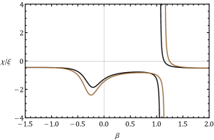
Figure 1: The behavior of dimensionless ratio $\chi/\xi$ in terms of exponent $\beta$ for epochs: RD (black curve) and MD (brown curve).

Concerning the Cosmological constant (current era) also one easily realizes that by setting $w=-1$, then a solution of (24) admits as solution $B(t)=constant$ [66]. Let us emphasize that, due to our interest in BBN and Baryogenesis epochs, throughout this paper, the last two cases are out of our attention, and the main concentration is the first case i.e., Eqs. (27) for the RD era.

At the end of this Section, we report the trace of the energy-momentum tensor of the bumblebee field in the FRW universe as follows

$$T^{(B)} = 4\kappa V+$$

$$+ 3B^{2}\Big{[}(\xi+\chi)\left(2H^{2}+{\textstyle{{\ddot{a}}\over{a}}}+4H{\textstyle{{\dot{B}}\over{B}}}\right)+$$

$$+ (\xi+2\chi)\left(H{\textstyle{{\dot{B}}\over{B}}}+{\textstyle{{{\dot{B}}^{2}}\over{B^{2}}}}+{\textstyle{{\ddot{B}}\over{B}}}\right)\Big{]}$$

$$= 4\kappa V+3b^{2}\Big{[}(\xi+\chi)\alpha(3\alpha+4\beta-1)+$$

$$+(\xi+2\chi)\beta(\alpha+2\beta-1)\Big{]}{\textstyle{{{\tilde{M}}^{2\beta}}\over{t^{2-2\beta}}}}\,.$$

The components $00$ and $ii$ of the energy-momentum tensor above address energy density and pressure arising from the presence of bumblebee vector fields in the background (see (56) to (A)). As the final word, in Appendix (C), ansatz (20) is supported by linear dynamic system analysis.

III BBN in bumblebee cosmology

In the Section, we examine the constraint on $\xi b^{2}$ coming from BBN. For our aim, the analysis here discussed to infer such a bound is enough.

BBN starts during the radiation dominated era [67, 68, 70]. The neutron abundance can be calculated via the conversion rate of protons into neutrons

$$\lambda_{pn}({T})=\lambda_{n+\nu_{e}\rightarrow p+e^{-}}+\lambda_{n+e^{+}\rightarrow p+{\bar{\nu}}_{e}}+\lambda_{n\rightarrow p+e^{-}+{\bar{\nu}}_{e}}\,,$$

and its inverse $\lambda_{np}({T})$, thus the total rate reads

$$\Lambda({T})=\lambda_{np}({T})+\lambda_{pn}({T})\,.$$ (31)

From (31) one gets (see (74))

$$\Lambda(T)=4A\,{T}^{3}(4!{T}^{2}+2\times 3!{\cal Q}{T}+2!{\cal Q}^{2})\,,$$ (32)

where ${\cal Q}$ stands for the difference between neutron and proton mass, ${\cal Q}=m_{n}-m_{p}$, while the numerical factor $A$ is given by $A=1.02\times 10^{-11}$GeV^-4. The ${}^{4}He$ primordial mass fraction is estimated by using the relation [67]

$$Y_{p}\equiv\lambda\,{\textstyle{{2x(t_{f})}\over{1+x(t_{f})}}}\,,$$ (33)

in which $\lambda=e^{-(t_{n}-t_{f})/\tau}$ ($t_{f}$ corresponds to the time of the freeze-out of the weak interactions, while $t_{n}$ to the time of the freeze-out of the nucleosynthesis), $\tau$ is the neutron mean lifetime defined in (72), and, finally, $x(t_{f})=e^{-{\cal Q}/{\cal T}(t_{f})}$ is the neutron-to-proton equilibrium ratio. The variation of the freezing temperature ${T}_{f}$ induces a deviation from the fractional mass $Y_{p}$ given by

$$\delta Y_{p}=Y_{p}\left[\left(1-{\textstyle{{Y_{p}}\over{2\lambda}}}\right)\ln\left({\textstyle{{2\lambda}\over{Y_{p}}}}-1\right)-{\textstyle{{2t_{f}}\over{\tau}}}\right]{\textstyle{{\delta{T}_{f}}\over{{T}_{f}}}}\,,$$ (34)

where $\delta{T}(t_{n})=0$ has been used (it comes from the fact that ${T}_{n}$ is fixed by the deuterium binding energy [71, 72]). Observations provide an estimation of $Y_{p}$ of baryon converted to ${}^{4}He$ given by [120, 121, 122, 123, 124, 125, 126]

$$Y_{p}=0.2476\,,\qquad|\delta Y_{p}|<10^{-4}\,.$$ (35)

Combining Eqs. (35) and (34) one gets

$$\left|{\textstyle{{\delta{T}_{f}}\over{{T}_{f}}}}\right|<4.7\times 10^{-4}\,.$$ (36)

For our aim, we rewrite the expansion rate of the BG-based universe at hand i.e., Eq. (12) in the form

$$H = H_{GR}\sqrt{1+{\textstyle{{\rho_{B}}\over{\kappa\rho}}}}\equiv H_{GR}+\delta H\,,$$ (37)

$$\delta H = H_{B}\equiv\left(\sqrt{1+{\textstyle{{\rho_{B}}\over{\kappa\rho}}}}-1\right)H_{GR}\,,$$ (38)

where $H_{GR}=\displaystyle{\sqrt{\kappa\rho}}$ is the expansion rate of the Universe in the standard cosmological model, ${\displaystyle\rho={\textstyle{{\pi^{2}}\over{30}}}g_{*}{T}^{4}}$, and $\rho_{B}$ is defined in (56). The relation $\Lambda=H$ gives the freeze-out temperature ${T}={T}_{f}\left(1+{\textstyle{{\delta{T}_{f}}\over{{T}_{f}}}}\right)$, with ${T}_{f}\sim 0.6$ MeV obtained from $H(T_{f})=\Lambda\simeq q{T_{f}}^{5}$, which $q\simeq 9.6\times 10^{-36}\,\text{GeV}^{-4}={\textstyle{{9.6\times 10^{40}}\over{M_{P}^{4}}}}$. Given that the deviation given raised of background bumblebee vector field from standard cosmology will lead to a deviation in the freeze-out temperature, thereby, by taking $\delta H=\delta H(T_{f})$ into account, we arrive at

$${\textstyle{{\delta{T}_{f}}\over{{T}_{f}}}}={\textstyle{{\left(\sqrt{1+{\textstyle{{\rho_{B}}\over{\kappa\rho}}}}-1\right)H_{GR}}\over{5q{T}_{f}^{5}}}}\simeq{\textstyle{{\rho_{B}}\over{\kappa\rho}}}{\textstyle{{H_{GR}}\over{10q{T}_{f}^{5}}}}\,,$$ (39)

The last term in (39) follows from this reasonable demand which $\rho_{B}\ll\rho$. We then get

$${\textstyle{{\rho_{B}}\over{\kappa\rho}}}=\xi b^{2}\Pi_{\xi,\chi}\left({\textstyle{{45}\over{16\pi^{3}g_{*}}}}\right)^{\beta}\left({\textstyle{{{\tilde{M}}M_{P}}\over{T_{f}^{2}}}}\right)^{2\beta}\,,$$ (40)

and

$${\textstyle{{H_{GR}}\over{10\,q\,T_{f}^{5}}}}={\textstyle{{1}\over{10}}}\sqrt{{\textstyle{{8\pi^{3}g_{*}}\over{30}}}}\,{\textstyle{{1}\over{qM_{P}T_{f}^{3}}}}={\textstyle{{10^{-40}}\over{48}}}\sqrt{{\textstyle{{\pi^{3}g_{*}}\over{15}}}}\,\left({\textstyle{{M_{P}}\over{T_{f}}}}\right)^{3}\,,$$ (41)

where $\Pi_{\xi,\chi}$ is defined as

$$\Pi_{\xi,\chi}\equiv-{\textstyle{{\left(1+{\textstyle{{\chi}\over{\xi}}}\right)(2\alpha\beta-2\alpha)+\left(1+2{\textstyle{{\chi}\over{\xi}}}\right)(8\beta^{2}-3\alpha\beta-4\beta)}\over{3(1+w)}}}\,.$$ (42)

Note that here we should set the values of $\alpha$ and $\chi/\xi$ from the RD epoch. By imposing the upper bound (36) on Eq. (39), in Figs. 2 and 3 (up rows) we illustrate the parameter space plots in terms of $\beta-\xi b^{2}$ which address the allowed regions in which the upper bound (36) satisfies. Also, in the bottom rows, we plot $\left|{\textstyle{{\delta{T}_{f}}\over{{T}_{f}}}}\right|$ in terms of $\xi b^{2}$ for optional values of $\beta$. As is evident, the upper bounds on $\xi b^{2}$ are sensitive to setting the value of exponent parameter $\beta$ ($B(t)\sim t^{\beta}$) so that for the negative case, the constraint on $\xi b^{2}$ is getting tighter as the value of $|\beta|$ gets smaller. For the case of $\beta>0$ also this statement works i.e., increasing the value of $\beta$ results in the upper bound on $\xi b^{2}$ shifts to lower ones. Concerning the negative case, for example by setting $\beta=-0.204$ one obtains the constraint $\lesssim 10^{-12}$ for $\xi b^{2}$, while for $\beta\approx-0.038$ it falls to range $\lesssim 10^{-24}$ which is $12$ order of magnitude more stringent than the former. As a result, it is expected that the corresponding upper bounds on $\xi b^{2}$ become even tighter than $10^{-24}$, if $\beta>-0.038$ (see the right panel in the bottom row of Fig. 2). Concerning the case $\beta>0$ a comment is in order. The values of $\beta>0$ imply that the bumblebee field grows with the cosmic time $t$, or, equivalently, increases as the temperature decreases. Despite that, this scenario guides us to tight upper bounds for $\xi b^{2}$ (see Fig. 3), they can not be reliable. In other words, these very tight constraints, in essence, come from the scenario that seems not cosmologically favourite since commonly one expects that the Lorentz violation terms are merely effective in the early universe, at high temperatures.

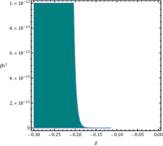
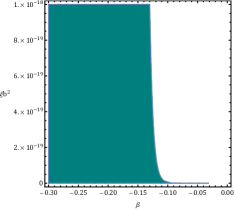
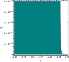
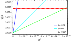
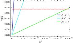
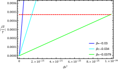
Figure 2: Up row: Regions of existence in the $\beta-\xi b^{2}$ parameter space which satisfies the upper bound (36). Bottom row: $\left|{\textstyle{{\delta{T}_{f}}\over{{T}_{f}}}}\right|$ from (39) in terms of $\xi b^{2}$ for optional values of $\beta$ which put in correspond allowed region. Here we set numerical values: ${\tilde{M}}\sim 10^{19}$GeV$\sim M_{P}$, $T_{f}\sim 6\times 10^{-4}$GeV, and $g_{*}=106.7$.

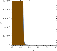
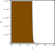
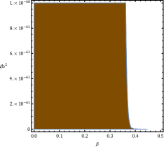
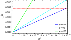
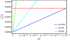
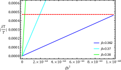
Figure 3: Same as the Fig. (2) but for $\beta>0$.

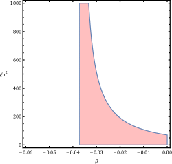
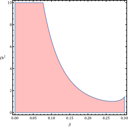
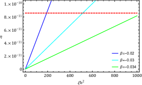
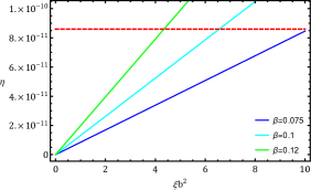
Figure 4: Up row: Regions of existence in the $\beta-\xi b^{2}$ parameter space which satisfies the constraint (53). Bottom row: $\eta$ from (52) in terms of $\xi b^{2}$ for optional values of $\beta$ which put in correspond allowed region. Here we set numerical values: ${\tilde{M}}=\bar{M}_{P}$= $M_{*}$, $T_{D}\sim 10^{16}$GeV, $g_{b}=2$ and $g_{*}\sim 107$.

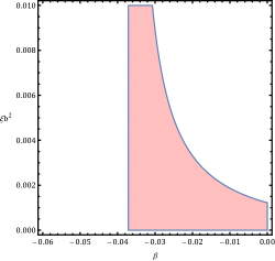
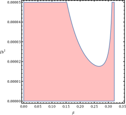
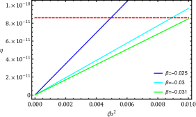
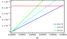
Figure 5: Same as the Fig. (4) but for $M_{*}\sim 10^{16}$GeV i.e., around GUT scale.

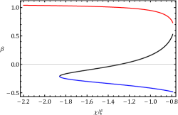
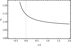
Figure 6: The behavior of exponent $\beta$ in terms of dimensionless ratio ${\textstyle{{\chi}\over{\xi}}}$ for RD epoch. The left and right panels dedicate to cases ${\textstyle{{\chi}\over{\xi}}}\leq-0.8$ with three real solutions (black, blue, and red), and ${\textstyle{{\chi}\over{\xi}}}>-0.8$ with just one real solution, respectively.

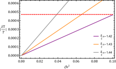
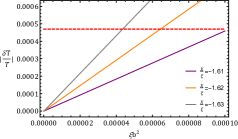
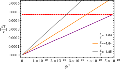
Figure 7: $\left|{\textstyle{{\delta{T}_{f}}\over{{T}_{f}}}}\right|$ from (39) in terms of $\xi b^{2}$ for some selected values of ${\textstyle{{\chi}\over{\xi}}}$ within the range $-1.85\leq{\textstyle{{\chi}\over{\xi}}}<-1.2$. The rest of the numerical values are equal to the same values in Fig. 2.

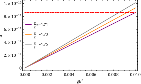
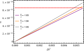
Figure 8: $\eta$ from (52) in terms of $\xi b^{2}$ for some selected values of ${\textstyle{{\chi}\over{\xi}}}$ within the range $-1.85\leq{\textstyle{{\chi}\over{\xi}}}<-1.2$. The rest of numerical values are equal to the same values in Fig. 5.

IV Gravitational baryogenesis in Bumblebee cosmology

In the light of supergravity theories there exist a mechanism for inducing baryon asymmetry during the evolution of the Universe, which has been proposed in [127, 128]. In this model, the thermal equilibrium is preserved, so that not all of Sakharov’s conditions are fulfilled. The interaction responsible for the (dynamical) CPT violation is given by [77]

$${\textstyle{{1}\over{M_{*}^{2}}}}\int\mathrm{d}^{4}x\sqrt{-g}\,J^{\mu}\partial_{\mu}R\,,$$ (43)

where $M_{*}$ is the cutoff scale characterizing the effective theory (typically it is of order reduced Planck mass $\bar{M}_{P}\sim 2.4\times 10^{18}$GeV), and $J^{\mu}$ the baron current (see Refs. [109, 110, 74, 111, 112, 113, 114, 115, 116, 117, 118] for further applications). In the vacuum, the interaction (43) violates $CP$, while $CPT$ is conserved. In an expanding universe, the interaction (43) dynamically breaks $CPT$, generating an energy shift that is responsible for the asymmetry between particles and antiparticles. Moreover, the existence of interactions that violate baryon processes in thermal equilibrium is essential so that a net baryon asymmetry can be generated and gets frozen at the decoupling temperature $T_{D}$. It, in essence, is the temperature at which the baryon asymmetry generating interactions happen and due to the fact that the expansion rate of the Universe is larger than the interaction rate, it remains fixed since the interaction is less frequent.

In an expanding universe, when the temperature drops below $T_{D}$, Eq. (43) conducts us to the following relation

$${\textstyle{{1}\over{M_{*}^{2}}}}J^{\mu}\partial_{\mu}R={\textstyle{{1}\over{M_{*}^{2}}}}(n_{B}-n_{\bar{B}})\dot{R}~{},$$ (44)

where ${\dot{R}}$, $n_{B}$, and $n_{\bar{B}}$ denote the time derivative of the Ricci scalar, baryon and anti-baryon number density, respectively. This relation allows defining the effective chemical potential for baryons $\mu_{B}$, and for anti-baryons $\mu_{\bar{B}}$, so that

$$\mu_{B}=-\mu_{\bar{B}}=-{\textstyle{{\dot{R}}\over{M_{*}^{2}}}}~{},$$ (45)

since (44) corresponds to the energy density term for a grand canonical ensemble. For relativistic particles, the net baryon number density reads [67]

$$n_{B}-n_{\bar{B}}={\textstyle{{g_{b}}\over{6}}}\mu_{B}T^{2}~{},$$ (46)

where $g_{b}\sim\mathcal{O}(1)$ is the number of intrinsic degrees of freedom of baryons. The above relations allow writing the parameter $\eta$ characterizing the baryon asymmetry in the following form [67]

$$\eta\equiv{\textstyle{{n_{B}-n_{\bar{B}}}\over{s}}}\approx{\textstyle{{n_{B}}\over{s}}}\simeq-{\textstyle{{15\,g_{b}}\over{4\pi^{2}g_{*}}}}{\textstyle{{\dot{R}}\over{M_{*}^{2}T}}}\bigg{|}_{T_{D}}~{},$$ (47)

where $s={\textstyle{{2\pi^{2}g_{*s}}\over{45}}}T^{3}$ is the entropy density (in the radiation-dominated era), and $g_{*s}\sim g_{*}\sim 107$ (here $g_{*s}$ is the number of degrees of freedom for particles which contribute to the entropy of the Universe, while $g_{*}$ the total number of degrees of freedom of relativistic particles [67].

As it arises from (47), $\eta$ is different from zero if $\dot{R}\neq 0$. As we are going to discuss, the presence of the bumblebee vector field in the background break thermal equilibrium and modifies $\dot{R}$, making it non-vanishing so that $\eta\neq 0$.

By reminding of GR, the Ricci scalar $\dot{R}$ is computed by the trace of Einstein field equations so that one gets $R=-\kappa\,{\cal T}=-\kappa\,(\rho-3p)$ (see Eq. (6)). In particular, during the radiation-dominated era, in which we are interested, the trace ${\cal T}$ vanishes (since the adiabatic index is $w=1/3$), meaning that $R=0$, and no net baryon asymmetry can be generated $\eta\sim{\dot{R}}=0$. This conclusion changes in the presence of a bumblebee background vector field. Actually, in such a case, the total energy-momentum is given by radiation and the bumblebee field $B$, so that the total trace does not vanish. As a results, Eq. (5) reads off

$$R=-T^{(B)}\,,$$ (48)

where $T^{(B)}$ is given in (II.1), so that

$$\dot{R}=-6N_{\xi,\chi}\xi b^{2}{\tilde{M}}^{3}\left({\tilde{M}}\,t\right)^{2\beta-3}\,,$$ (49)

with

$$N_{\xi,\chi} = \left(1+{\textstyle{{\chi}\over{\xi}}}\right)(\beta-1)(3\alpha^{2}+4\alpha\beta-\alpha)+$$

$$+ \left(1+2{\textstyle{{\chi}\over{\xi}}}\right)\left(2\beta^{2}+\alpha\beta-\beta\right)+$$

$$+ 2\alpha\beta\left((2\alpha^{2}+2\alpha-2){\textstyle{{\chi}\over{\xi}}}+\alpha-1\right)\,.$$

Note that the above equations are obtained by using Eq. (II.1). We recall that during the RD era the cosmic time $t$ and the temperature $T$ are related as

$${\displaystyle{\textstyle{{1}\over{t}}}\simeq({\textstyle{{4\pi^{2}g_{*}}\over{90}}})^{1/2}{\textstyle{{{T}^{2}}\over{\bar{M}_{P}}}}}\,,$$ (51)

or, equivalently ${T}(t)\simeq(t/\text{sec})^{-1/2}$MeV (notice that the entropy conservation $S\sim a^{3}{T}^{3}=constant$ implies $T(t)a(t)=T_{0}a_{0}$, where $T_{0}$ and $a_{0}$ are the temperature and scale factor of the Universe, $T_{0}\simeq 10^{-4}$eV, $a_{0}=1$, respectively). By substituting (49) in the baryon asymmetry formula (47), one obtains

$$\eta=\varpi\,{N}_{\xi,\chi}\xi b^{2}\,\left({\textstyle{{\tilde{M}}\over{M_{*}}}}\right)^{2}\left({\textstyle{{T_{D}}\over{\bar{M}_{P}}}}\right)^{3-2\beta}\left({\textstyle{{T_{D}}\over{{\tilde{M}}}}}\right)^{2-2\beta}\,,$$ (52)

where the constant $\varpi$ is given by

$$\varpi\equiv g_{b}\left({\textstyle{{2\pi^{2}g_{*}}\over{45}}}\right)^{(1-2\beta)/2}\,.$$

Now, using the bound on the baryon asymmetry parameter $\eta$, that is [107, 108]

$$0<\eta\lesssim\eta_{obs}\sim 8.6\times 10^{-11}\,,$$ (53)

we can extract some explicit constraints on $\xi b^{2}$ in interplay with negative and positive values of exponent parameter $\beta$.

Now, by imposing the above-mentioned constraint on Eq. (52), in Fig. 4 (up row) we illustrate the parameter space plots in terms of $\beta-\xi b^{2}$ which address the allowed regions in which the upper bound (53) is satisfied. Also, in the bottom row of this figure, we draw the plots $\eta-\xi b^{2}$ for some values of $\beta$ which are put in the corresponding allowed region. Concerning the case $\beta<0$ we find that independent of value of $\xi b^{2}$, for $\beta\leq-0.038$, the baryon asymmetry parameter becomes negative which is meaningless and not acceptable. So, by adopting range $-0.038<\beta<0$, one can extract some upper bounds around $10^{2-3}$ for $\xi b^{2}$. As one can see, by going to the case $\beta>0$ this upper bound will improve a few orders of magnitude.

An interesting result we found here is that the cutoff scale $M_{*}$ plays an inevitable role in falling the upper bounds on $\xi b^{2}$. As we can see from Fig. 4 there we have fixed $M_{*}=\bar{M}_{P}$, corresponding to the Planck scales at which the interaction (47) is effective. In essence, we deal with an effective theory, and fix $M_{*}$ a few orders of magnitude lower e.g., around the GUT scale ($M_{*}\sim 10^{16}$GeV). In this case, the upper bounds released for $\xi b^{2}$ in Fig. 4 improve a few orders of magnitude, see Fig. 5. Despite these improvements, in comparison with upper bounds extracted from BBN in the previous section, we still do not deal with stringent constraints on $\xi b^{2}$. Indeed, the achievement worth of noting here is not related to the upper bound derived for $\xi b^{2}$, but is for restricting the evolution rate of the bumblebee vector field i.e., $-0.038<\beta<0$. The worth of this constraint is to consider it complementary to BBN, in the sense that other values belonging to the $\beta\leq-0.038$ range in BBN analysis are ruled out. In this way, the most conservative constraint extracted within the range $-0.038<\beta<0$ for the VEV of the bumblebee timelike vector field i.e., $\xi b^{2}$ is $\lesssim 10^{-24}$. We say the most conservative since for all values except for $\beta=-0.038$ within the allowed range of $\beta$, the above-mentioned upper bound gets tighter, as one can see of Fig. 2 (the right panel in the bottom row).

V New strategy: Constraints on $\xi b^{2}$ in interplay with ${\textstyle{{\chi}\over{\xi}}}$

So far, all constraints derived for $\xi b^{2}$ from BBN and Baryogenesis come, in essence, from the interplay with exponent $\beta$. More exactly, by solving Eq. (26) in terms of ${\textstyle{{\chi}\over{\xi}}}$ for RD era, we indeed treated $\beta$ as a free parameter. The benefit of this approach is that it lets us probe $\xi b^{2}$ in explicit interplay with the free parameter $\beta$ related to the evolution of the bumblebee field in the RD era. Alternatively, there is another possibility in which Eq. (26) is solved in terms of $\beta$ and, subsequently, the dimensionless ratio ${\textstyle{{\chi}\over{\xi}}}$ this time is treated as the involved parameter. This gives us the possibility of probing $\xi b^{2}$ in explicit interplay with ${\textstyle{{\chi}\over{\xi}}}$ as coupling constants in the action (1).

By solving Eq. (26) for RD era in terms of $\beta$, we have a cubic equation such as

$$\beta^{3}-\bigg{(}{\textstyle{{7+18{\textstyle{{\chi}\over{\xi}}}}\over{16+32{\textstyle{{\chi}\over{\xi}}}}}}\bigg{)}\beta^{2}-\bigg{(}{\textstyle{{9+14{\textstyle{{\chi}\over{\xi}}}}\over{16+32{\textstyle{{\chi}\over{\xi}}}}}}\bigg{)}\beta-\bigg{(}{\textstyle{{9+7{\textstyle{{\chi}\over{\xi}}}}\over{32+64{\textstyle{{\chi}\over{\xi}}}}}}\bigg{)}=0.$$ (54)

It is not difficult to show that the cubic equation above for ${\textstyle{{\chi}\over{\xi}}}\leq-0.8$ has three real solutions, while it has just one real solution for ${\textstyle{{\chi}\over{\xi}}}>-0.8$. We display both cases in Fig. 6. It is observed that just two solutions marked with black and blue curves in the left panel, address $\beta<0$ (as the desirable case of cosmology, as already stated). The range $-1.85\leq{\textstyle{{\chi}\over{\xi}}}<-1.2$ is the common region of ${\textstyle{{\chi}\over{\xi}}}$ for these two solutions. Now, by taking into account the solution marked with the blue curve in Fig. 6 and using the BBN constraint (39), we can plot $\left|{\textstyle{{\delta{T}_{f}}\over{{T}_{f}}}}\right|$ in terms of $\xi b^{2}$ for values of ${\textstyle{{\chi}\over{\xi}}}$ within the aforementioned range, see Fig 7. It can be seen that the upper bound of $\xi b^{2}$ moves from $10^{-2}$ to $10^{-10}$, as the value of the dimensionless ratio ${\textstyle{{\chi}\over{\xi}}}$ approaches its extreme one i.e., $-1.85$. So, it is easy to recognize that for values $-1.2\leq{\textstyle{{\chi}\over{\xi}}}<-0.8$, we will deal with the resulting very weak upper bounds for $\xi b^{2}$.

In this regard, by putting the favored solution of $\beta$ (corresponding to the blue curve in Fig. 6) into the baryon asymmetry parameter $\eta$ in Eq. (52), we display in Fig. 8 the plot of $\eta-\xi b^{2}$ for some selecting values of ${\textstyle{{\chi}\over{\xi}}}$. Here, the best upper bound for $\xi b^{2}$, which is not better than the order of magnitude $10^{-3}$, extracts by setting ${\textstyle{{\chi}\over{\xi}}}$ around the extreme value.

Now, one can compare quantitatively the upper bounds obtained here for $\xi b^{2}$ and those were derived in the two previous Sections. One can infer that despite the constraints obtained from Baryogenesis in both approaches having almost the same order of magnitude, for BBN the former approach is more efficient since results in deriving tighter constraints on $\xi b^{2}$.

VI Conclusions

In this paper, we have considered a vector extension of the standard cosmology known as the bumblebee model in which by keeping isotropy and homogeneity of the Universe, the Lorentz symmetry spontaneously breaks by coupling a background time-like bumblebee vector field to Ricci tensor and scalar. We have used the implication of this cosmology model at hand for the formation of light elements and baryon asymmetry in the early universe, namely on the Big Bang Nucleosynthesis (BBN) and Baryogenesis respectively. By taking into account of a time-depending ansatz $\sim t^{\beta}$ for the evolution of the bumblebee field $B(t)$ with cosmic time, we in Sections III and IV have extracted some upper bounds on the vacuum expectation value (VEV) of the bumblebee timelike vector field i.e. $\xi b^{2}$. By solving Eq. (26) in terms of the dimensionless ratio ${\textstyle{{\chi}\over{\xi}}}$, we have analyzed both possible negative and positive ranges of exponent parameter $\beta$, with particular attention to the former, since it addresses the diluting of the bumblebee field as the Universe evolves, which is favored from the view of cosmology. From the combination of BBN and Baryogenesis, we find that, for the favourite scenario of the time-depending bumblebee vector field with a negative exponent parameter, the constraints are: $-0.038<\beta<0$, and $\xi b^{2}\lesssim 10^{-24}$. It is important to note that the above upper bound on $\xi b^{2}$ is derived in the case of setting $\beta\approx-0.038$, so that by going to within the allowed range of $\beta$, the upper bound gets a few orders of magnitude tighter.

At the end of our analysis (Section V), we pursued the strategy of solving Eq. (26) in terms of $\beta$. It lets us probe $\xi b^{2}$ this time in explicit interplay with the ratio ${\textstyle{{\chi}\over{\xi}}}$ made by two coupling constants embedded in the action (1). We have repeated the same analysis done in Sections related to BBN, and Baryogenesis, and derived some upper bounds for $\xi b^{2}$. The comparison of upper bounds in Section V with previous counterparts openly shows that the most stringent constraints for $\xi b^{2}$ come from the primary strategy in Sections III and IV.

Referring to II, in particular to the connection between the exponent parameter $\beta$ and the general power-law form of the bumblebee potential $\left(B^{\mu}B_{\mu}\pm b^{2}\right)^{n}$, there is a relation given by $\beta={\textstyle{{-1}\over{n-1}}}$. As a consequence, the tight constraint $-0.038<\beta<0$ implies that the power-law bumblebee potential of the form $\left(B^{\mu}B_{\mu}\pm b^{2}\right)^{n\leq 27}$ is ruled out. Concerning the new strategy, we saw that the favorite solution of Eq. (26) i.e., the blue curve in the left panel of Fig. (6), restricts the exponent parameter within the range $-0.47<\beta\leq-0.22$, corresponding to $3.12<n\leq 5.5$. Overall, in light of both approaches, one should no longer worry about the instability issue raised in [47] for the existing cosmological model.

Finally, it is worth mentioning the significance of the results. First of all, very stringent constraints derived for $\xi b^{2}$ from BBN indicate the size of Lorentz violation for the early Universe with the same course of evolution expected from standard cosmology. In other words, these constraints have been obtained provided that the BBN predictions are preserved. Second, unlike the standard cosmological model, by taking the BG model into account, the gravitational baryogenesis mechanism allows for explaining the matter-antimatter asymmetry in the Universe induced by the bumblebee field.

Appendix A Useful formulas

In this Appendix, we report some useful formulas. For the power law dependence of the scale factor, $a(t)=a_{0}t^{\alpha}$, one has

$${\textstyle{{\dot{a}}\over{a}}}={\textstyle{{\alpha}\over{t}}}\,,\quad{\textstyle{{\ddot{a}}\over{a}}}={\textstyle{{\alpha(\alpha-1)}\over{t^{2}}}}\,,\quad{\textstyle{{\dddot{a}}\over{a}}}={\textstyle{{\alpha(\alpha-1)(\alpha-2)}\over{t^{3}}}}\,.$$ (55)

The components of the energy-momentum tensor of the bumblebee field are given by

$$T^{(B)0}_{\quad\quad 0} = \kappa V+3B^{2}H\left((\xi+\chi)H+(\xi+2\chi){\textstyle{{\dot{B}}\over{B}}}\right)$$ (56)

$$\equiv \rho_{B}\,,$$

$$T^{(B)i}_{\quad\quad j} = \Big{\{}\kappa V+B^{2}\Big{[}(\xi+\chi)\left(H^{2}+{\textstyle{{\ddot{a}}\over{a}}}+4H{\textstyle{{\dot{B}}\over{B}}}\right)+$$ (57)

$$+(\xi+2\chi)\left({\textstyle{{{\dot{B}}^{2}}\over{B^{2}}}}+{\textstyle{{\ddot{B}}\over{B}}}\right)\Big{]}\Big{\}}\delta^{i}_{j}$$

$$\equiv -p_{B}\,\delta^{i}_{j}\,.$$

Using (20) one gets that in a FRW universe $\rho_{B}$ and $p_{B}$, Eqs. (56) and (57), are given by

$$\rho_{B} = \kappa V+3b_{0}^{2}\alpha[(\xi+\chi)\alpha+(\xi+2\chi)\beta]{\textstyle{{{\tilde{M}}^{2\beta}}\over{t^{2-2\beta}}}}\,,$$ (58)

$$p_{B} = -\kappa V-b_{0}^{2}\Big{[}(\xi+\chi)\alpha(2\alpha-1+4\beta)+$$

$$+(\xi+2\chi)\beta(2\beta-1)\Big{]}{\textstyle{{{\tilde{M}}^{2\beta}}\over{t^{2-2\beta}}}}\,.$$

Moreover,

$${\dot{\rho}}_{B}=b_{0}^{2}3\alpha(B_{B}-A_{B})\,{\textstyle{{{\tilde{M}}^{2\beta}}\over{t^{3-2\beta}}}}\,,$$

where $A_{B}$ and $B_{B}$ are defined in (22a) and (22b).

Appendix B Big Bang Nucleosynthesis

We shortly review the main features of BBN [67, 68]. In the early universe, the primordial ${}^{4}He$ was formed at temperature ${T}\sim{\cal O}(1)$ MeV. The (relativistic) electron, positron, neutrinos and photons are in thermal equilibrium owing to the rapid collision. The interactions involved are $\nu_{e}+n\leftrightarrow p+e^{-}$, $e^{+}+n\leftrightarrow p+{\bar{\nu}}_{e}$ and $n\leftrightarrow p+e^{-}+{\bar{\nu}}_{e}$. The neutron abundance is computed via the conversion rate of protons into neutrons ($\lambda_{pn}$) and its inverse ($\lambda_{np}$)

$$\Lambda({T})=\lambda_{np}({T})+\lambda_{pn}({T})\,,$$ (60)

where

$$\lambda_{np}=\lambda_{n+\nu_{e}\rightarrow p+e^{-}}+\lambda_{n+e^{+}\rightarrow p+{\bar{\nu}}_{e}}+\lambda_{n\rightarrow p+e^{-}+{\bar{\nu}}_{e}}\,.$$ (61)

The rates $\lambda_{np}$ and $\lambda_{pn}$ are related as $\lambda_{np}({T})=e^{-{\cal Q}/{T}}\lambda_{pn}({T})$, with ${\cal Q}=m_{n}-m_{p}$ the mass difference of neutron and proton. The interaction rate for the process $n+\nu_{e}\rightarrow p+e^{-}$ is

$$d\lambda_{n+\nu_{e}\rightarrow p+e^{-}}=d\mu\,|\langle{\cal M}|^{2}\rangle W\,,$$ (62)

where the various terms are defined as

$$d\mu \equiv {\textstyle{{d^{3}p_{e}}\over{(2\pi)^{3}2E_{e}}}}{\textstyle{{d^{3}p_{\nu_{e}}}\over{(2\pi)^{3}2E_{\nu_{e}}}}}{\textstyle{{d^{3}p_{p}}\over{(2\pi)^{3}2E_{p}}}}\,,$$ (63)

$$W \equiv (2\pi)^{4}\delta^{(4)}({\cal P})n(E_{\nu_{e}})[1-n(E_{e})]\,,$$ (64)

$${\cal P} \equiv p_{n}+p_{\nu_{e}}-p_{p}-p_{e}\,,$$ (65)

$${\cal M} = \left({\textstyle{{g_{w}}\over{8M_{W}}}}\right)^{2}[{\bar{u}}_{p}\Omega^{\mu}u_{n}][{\bar{u}}_{e}\Sigma_{\mu}v_{\nu_{e}}]\,,$$ (66)

$$\Omega^{\mu} \equiv \gamma^{\mu}(c_{V}-c_{A}\gamma^{5})\,,$$ (67)

$$\Sigma^{\mu} \equiv \gamma^{\mu}(1-\gamma^{5})\,.$$ (68)

From Eq. (62) one gets

$$\lambda_{n+\nu_{e}\rightarrow p+e^{-}}=A\,{\cal T}^{5}I_{y}\,,$$ (69)

where $A\equiv{\textstyle{{g_{V}+3g_{A}}\over{2\pi^{3}}}}$ and

$$I_{y}=\int_{y}^{\infty}\epsilon(\epsilon-{\cal Q}^{\prime})^{2}\sqrt{\epsilon^{2}-y^{2}}\,n(\epsilon-{\cal Q})[1-n(\epsilon)]d\epsilon,$$ (70)

with $y\equiv{\textstyle{{m_{e}}\over{{T}}}}$ and ${\cal Q}^{\prime}={\textstyle{{{\cal Q}}\over{{T}}}}$. In a similar way, for the process $e^{+}+n\rightarrow p+{\bar{\nu}}_{e}$, one gets

$$\lambda_{e^{+}+n\rightarrow p+{\bar{\nu}}_{e}}=A\,{T}^{3}(4!{T}^{2}+2\times 3!{\cal Q}{T}+2!{\cal Q}^{2})\,.$$ (71)

Finally, the neutron decay follows from $n\rightarrow p+e^{-}+{\bar{\nu}}_{e}$, giving

$$\tau=\lambda_{n\rightarrow p+e^{-}+{\bar{\nu}}_{e}}^{-1}\simeq 887\text{sec}\,.$$ (72)

In (61) one can safely neglect the contribution (72) (during the BBN the neutron can be considered as a stable particle) [68]. Following [68] one can show that $\lambda_{e^{+}+n\rightarrow p+{\bar{\nu}}_{e}}=\lambda_{n+\nu_{e}\rightarrow p+e^{-}}$. Inserting these results into (61) and (60), one infers

$$\Lambda({T})\simeq 2\lambda_{np}=4\lambda_{e^{+}+n\rightarrow p+{\bar{\nu}}_{e}}\,,$$ (73)

which yields (using (71))

$$\Lambda({\cal T})=4A\,{T}^{3}(4!{T}^{2}+2\times 3!{\cal Q}{T}+2!{\cal Q}^{2})\,.$$ (74)

Appendix C Linear stability analysis of ansatz (20)

Given that ansatz (20) plays a key role in the description of the BBN and the gravitational baryogenesis so it is essential to investigate whether it is an attractor solution or not. In the language of dynamical systems theory, attractor address situations where a collection of points in phase-space evolve within a given region, without leaving it. In other words, these points are stable in phase-space because them behave as sink or spiral sink. So, the advantage of an attractor solution is that it does not suffer from a fine-tuning of the initial conditions.

To do so, putting ansatz (20) in the form $B=ba^{2\beta}$, together with introducing new variables $X_{1}=a$, and $X_{2}=\dot{a}$ in (II.1), we reduce this second order dynamic equation to the following first order, consist of a autonomous system of differential equations

$$\dot{X}_{1} = X_{2}=\mathcal{F}_{1}(X_{1},X_{2})~{},$$

$$\dot{X}_{2} = {\textstyle{{2X_{2}^{2}}\over{({\textstyle{{\chi}\over{\xi}}}+1)X_{1}^{4\beta+1}+2X_{1}}}}-{\textstyle{{g_{1}X_{1}^{4\beta-2}}\over{({\textstyle{{\chi}\over{\xi}}}+1)X_{1}^{4\beta+1}+2X_{1}}}}$$ (75)

$$+{\textstyle{{g_{2}X_{1}^{4\beta}X_{2}^{2}}\over{({\textstyle{{\chi}\over{\xi}}}+1)X_{1}^{4\beta+1}+2X_{1}}}}-{\textstyle{{4}\over{3({\textstyle{{\chi}\over{\xi}}}+1)X_{1}^{4\beta+3}+6X_{1}^{3}}}}=$$

$$\mathcal{F}_{2}(X_{1},X_{2}),$$

where

$$g_{1}= {\textstyle{{\xi b^{2}(\beta(24{\textstyle{{\chi}\over{\xi}}}+14)+7{\textstyle{{\chi}\over{\xi}}}+9)}\over{4\beta}}},$$ (76a)

$$g_{2}= \xi b^{2}\left(48\beta^{2}(2{\textstyle{{\chi}\over{\xi}}}+1)-\beta(36{\textstyle{{\chi}\over{\xi}}}+14)-2({\textstyle{{\chi}\over{\xi}}}+1)\right).$$ (76b)

Note that to derive of equations above, we have set $\omega=1/3$, and $\alpha=1/2$ together with $a_{0}=\tilde{M}=\kappa=1$. Now by serving the Jacobian matrix for the autonomous system (C)

$$J\bigg{(}\mathcal{F}_{1}(X_{1},X_{2}),\mathcal{F}_{2}(X_{1},X_{2})\bigg{)}=\left(\begin{array}[]{cc}{\textstyle{{\partial\mathcal{F}_{1}}\over{\partial X_{1}}}}&{\textstyle{{\partial\mathcal{F}_{1}}\over{\partial X_{2}}}}\\ {\textstyle{{\partial\mathcal{F}_{2}}\over{\partial X_{1}}}}&{\textstyle{{\partial\mathcal{F}_{2}}\over{\partial X_{2}}}}\\ \end{array}\right)$$ (79)

we can say whether the solution (20) within phase-space $(X_{1},X_{2})$ can be an attractor or not. More precisely, the Jacobian matrix (79) is stable, indicating the solution (20) is an attractor provided that its trace and determinant i.e.,

$$tr={\textstyle{{\partial\mathcal{F}_{2}}\over{\partial X_{2}}}},~{}~{}~{}\mbox{and}~{}~{}~{}det=-{\textstyle{{\partial\mathcal{F}_{2}}\over{\partial X_{1}}}},~{}~{}~{}\mbox{where}~{}~{}~{}$$

$${\textstyle{{\partial\mathcal{F}_{1}}\over{\partial X_{1}}}}=0,~{}~{}~{}~{}{\textstyle{{\partial\mathcal{F}_{1}}\over{\partial X_{2}}}}=1$$ (80)

are negative and positive, respectively [130]. By deriving ${\textstyle{{\partial\mathcal{F}_{2}}\over{\partial X_{1}}}}$, and ${\textstyle{{\partial\mathcal{F}_{2}}\over{\partial X_{2}}}}$, after some straightforward algebraic calculations, one can show that for ${\textstyle{{\chi}\over{\xi}}}<0$, and $\beta<0$, we have $tr<0$, and $det>0$, meaning that ansatz (20), enjoys stability and address an attractor solution.

References

- [1] V. A. Kostelecky and S. Samuel, Phys. Rev. Lett. 66, 1811-1814 (1991)
- [2] V. A. Kostelecky and R. Potting, Phys. Rev. D 51, 3923-3935 (1995) [arXiv:hep-ph/9501341 [hep-ph]].
- [3] D. Colladay and V. A. Kostelecky, Phys. Rev. D 55, 6760-6774 (1997) [arXiv:hep-ph/9703464 [hep-ph]].
- [4] D. Colladay and V. A. Kostelecky, Phys. Rev. D 58, 116002 (1998) [arXiv:hep-ph/9809521 [hep-ph]].
- [5] V. A. Kostelecky, Phys. Rev. D 69, 105009 (2004) [arXiv:hep-th/0312310 [hep-th]].
- [6] R. Bluhm and V. A. Kostelecky, Phys. Rev. D 71, 065008 (2005) [arXiv:hep-th/0412320 [hep-th]].
- [7] V. A. Kostelecky and R. Potting, Gen. Rel. Grav. 37, 1675-1679 (2005) [arXiv:gr-qc/0510124 [gr-qc]].
- [8] V. A. Kostelecky and N. Russell, Rev. Mod. Phys. 83, 11-31 (2011) [arXiv:0801.0287 [hep-ph]].
- [9] S. M. Carroll, J. A. Harvey, V. A. Kostelecky, C. D. Lane and T. Okamoto, Phys. Rev. Lett. 87, 141601 (2001) [arXiv:hep-th/0105082 [hep-th]].
- [10] D. Mattingly, Living Rev. Rel. 8, 5 (2005) [arXiv:gr-qc/0502097 [gr-qc]].
- [11] G. Amelino-Camelia, Living Rev. Rel. 16, 5 (2013) [arXiv:0806.0339 [gr-qc]].
- [12] S. Liberati, Class. Quant. Grav. 30, 133001 (2013) [arXiv:1304.5795 [gr-qc]].
- [13] V. A. Kostelecky and C. D. Lane, J. Math. Phys. 40, 6245-6253 (1999) [arXiv:hep-ph/9909542 [hep-ph]].
- [14] T. J. Yoder and G. S. Adkins, Phys. Rev. D 86, 116005 (2012) [arXiv:1211.3018 [hep-ph]].
- [15] R. Lehnert, Phys. Rev. D 68, 085003 (2003) [arXiv:gr-qc/0304013 [gr-qc]].
- [16] V. A. Kostelecky and M. Mewes, Phys. Rev. Lett. 87, 251304 (2001) [arXiv:hep-ph/0111026 [hep-ph]].
- [17] V. A. Kostelecky and M. Mewes, Phys. Rev. D 66, 056005 (2002) [arXiv:hep-ph/0205211 [hep-ph]].
- [18] V. A. Kostelecky and M. Mewes, Phys. Rev. Lett. 97, 140401 (2006) [arXiv:hep-ph/0607084 [hep-ph]].
- [19] S. M. Carroll, G. B. Field and R. Jackiw, Phys. Rev. D 41, 1231 (1990)
- [20] M. A. Hohensee, R. Lehnert, D. F. Phillips and R. L. Walsworth, Phys. Rev. D 80, 036010 (2009) [arXiv:0809.3442 [hep-ph]].
- [21] F. R. Klinkhamer and M. Schreck, Nucl. Phys. B 848, 90-107 (2011) [arXiv:1011.4258 [hep-th]].
- [22] M. Schreck, Phys. Rev. D 86, 065038 (2012) [arXiv:1111.4182 [hep-th]].
- [23] D. Colladay and P. McDonald, Phys. Rev. D 79, 125019 (2009) [arXiv:0904.1219 [hep-ph]].
- [24] V. E. Mouchrek-Santos and M. M. Ferreira, Phys. Rev. D 95, no.7, 071701 (2017) [erratum: Phys. Rev. D 100, no.9, 099901 (2019)] [arXiv:1611.05336 [hep-ph]].
- [25] Q. G. Bailey and V. A. Kostelecky, Phys. Rev. D 74, 045001 (2006) [arXiv:gr-qc/0603030 [gr-qc]].
- [26] T. Jacobson and D. Mattingly, Phys. Rev. D 64, 024028 (2001) [arXiv:gr-qc/0007031 [gr-qc]].
- [27] R. V. Maluf, V. Santos, W. T. Cruz and C. A. S. Almeida, Phys. Rev. D 88, no.2, 025005 (2013) [arXiv:1304.2090 [hep-th]].
- [28] R. V. Maluf, C. A. S. Almeida, R. Casana and M. M. Ferreira, Jr., Phys. Rev. D 90, no.2, 025007 (2014) [arXiv:1402.3554 [hep-th]].
- [29] R. Bluhm and V. A. Kostelecky, Phys. Rev. D 71, 065008 (2005) [arXiv:hep-th/0412320 [hep-th]].
- [30] R. Bluhm, S. H. Fung and V. A. Kostelecky, Phys. Rev. D 77, 065020 (2008) [arXiv:0712.4119 [hep-th]].
- [31] B. Altschul and V. A. Kostelecky, Phys. Lett. B 628, 106-112 (2005) [arXiv:hep-th/0509068 [hep-th]].
- [32] R. Bluhm, [arXiv:1302.2278 [hep-th]].
- [33] V. A. Kostelecky and R. Potting, Phys. Rev. D 79, 065018 (2009) [arXiv:0901.0662 [gr-qc]].
- [34] V. A. Kostelecky and R. Potting, Gen. Rel. Grav. 37, 1675-1679 (2005) [arXiv:gr-qc/0510124 [gr-qc]].
- [35] A. V. Kostelecky and J. D. Tasson, Phys. Rev. D 83, 016013 (2011) [arXiv:1006.4106 [gr-qc]].
- [36] M. Khodadi and E. N. Saridakis, Phys. Dark Univ. 32, 100835 (2021) [arXiv:2012.05186 [gr-qc]].
- [37] M. Khodadi and G. Lambiase, Phys. Rev. D 106, no.10, 104050 (2022) [arXiv:2206.08601 [gr-qc]].
- [38] V. A. Kostelecký, A. C. Melissinos and M. Mewes, Phys. Lett. B 761, 1-7 (2016) [arXiv:1608.02592 [gr-qc]].
- [39] V. A. Kostelecký and M. Mewes, Phys. Lett. B 757, 510-514 (2016) [arXiv:1602.04782 [gr-qc]].
- [40] T. Jacobson and D. Mattingly, Phys. Rev. D 64, 024028 (2001) [arXiv:gr-qc/0007031 [gr-qc]].
- [41] R. Bluhm and V. A. Kostelecky, Phys. Rev. D 71, 065008 (2005) [arXiv:hep-th/0412320 [hep-th]].
- [42] O. Bertolami and J. Paramos, Phys. Rev. D 72, 044001 (2005) [arXiv:hep-th/0504215 [hep-th]].
- [43] V. A. Kostelecky and S. Samuel, Phys. Rev. D 40, 1886-1903 (1989)
- [44] M. D. Seifert, Phys. Rev. D 81, 065010 (2010) [arXiv:0909.3118 [hep-ph]].
- [45] O. Bertolami and J. Paramos, Phys. Rev. D 72, 044001 (2005) [arXiv:hep-th/0504215 [hep-th]].
- [46] A. Crivellin, F. Kirk and M. Schreck, [arXiv:2208.11420 [hep-ph]].
- [47] R. Bluhm, N. L. Gagne, R. Potting and A. Vrublevskis, Phys. Rev. D 77, 125007 (2008) [erratum: Phys. Rev. D 79, 029902 (2009)] [arXiv:0802.4071 [hep-th]].
- [48] D. Liang, R. Xu, X. Lu and L. Shao, [arXiv:2207.14423 [gr-qc]].
- [49] C. Liu, C. Ding and J. Jing, [arXiv:1910.13259 [gr-qc]].
- [50] C. Ding, C. Liu, R. Casana and A. Cavalcante, Eur. Phys. J. C 80, no.3, 178 (2020) [arXiv:1910.02674 [gr-qc]].
- [51] S. Chen, M. Wang and J. Jing, JHEP 07, 054 (2020) [arXiv:2004.08857 [gr-qc]].
- [52] R. V. Maluf and J. C. S. Neves, Phys. Rev. D 103, no.4, 044002 (2021) [arXiv:2011.12841 [gr-qc]].
- [53] S. Kanzi and İ. Sakallı, Eur. Phys. J. C 81, no.6, 501 (2021) [arXiv:2102.06303 [hep-th]].
- [54] M. Khodadi, Phys. Rev. D 103, no.6, 064051 (2021) [arXiv:2103.03611 [gr-qc]].
- [55] M. Khodadi, Phys. Rev. D 105, no.2, 023025 (2022) [arXiv:2201.02765 [gr-qc]].
- [56] A. Delhom, T. Mariz, J. R. Nascimento, G. J. Olmo, A. Y. Petrov and P. J. Porfírio, JCAP 07, no.07, 018 (2022) [arXiv:2202.11613 [hep-th]].
- [57] R. V. Maluf and C. R. Muniz, Eur. Phys. J. C 82, no.1, 94 (2022) [arXiv:2202.01015 [gr-qc]].
- [58] S. K. Jha and A. Rahaman, Eur. Phys. J. C 82, no.5, 411 (2022) [arXiv:2203.08099 [gr-qc]].
- [59] X. M. Kuang and A. Övgün, [arXiv:2205.11003 [gr-qc]].
- [60] A. Carleo, G. Lambiase and L. Mastrototaro, Eur. Phys. J. C 82, no.9, 776 (2022) [arXiv:2206.12988 [gr-qc]].
- [61] M. Khodadi, G. Lambiase and L. Mastrototaro, Eur. Phys. J. C 83, no.3, 239 (2023) [arXiv:2302.14200 [hep-ph]].
- [62] R. V. Maluf and J. C. S. Neves, JCAP 10, 038 (2021) [arXiv:2105.08659 [gr-qc]].
- [63] J. Páramos and G. Guiomar, Phys. Rev. D 90, no.8, 082002 (2014) [arXiv:1409.2022 [astro-ph.SR]].
- [64] R. Casana, A. Cavalcante, F. P. Poulis and E. B. Santos, Phys. Rev. D 97, no.10, 104001 (2018) [arXiv:1711.02273 [gr-qc]].
- [65] R. Xu, D. Liang and L. Shao, Phys. Rev. D 107, no.2, 024011 (2023) [arXiv:2209.02209 [gr-qc]].
- [66] D. Capelo and J. Páramos, Phys. Rev. D 91, no.10, 104007 (2015) [arXiv:1501.07685 [gr-qc]].
- [67] E.W. Kolb, M.S. Turner, The Early Universe , Addison Wesley Publishing Company, (1989).
- [68] J. Bernstein, L. S. Brown and G. Feinberg, Rev. Mod. Phys. 61, 25 (1989)
- [69] S. Burles, K. M. Nollett and M. S. Turner, Phys. Rev. D 63, 063512 (2001) [arXiv:astro-ph/0008495 [astro-ph]].
- [70] K. A. Olive et al. [Particle Data Group], Chin. Phys. C 38, 090001 (2014)
- [71] D.F. Torres, H. Vucetich, A. Plastino, Phys. Rev. Lett. 79, 1588 (1997).
- [72] S. Capozziello, G. Lambiase and E. N. Saridakis, Eur. Phys. J. C 77, no.9, 576 (2017) [arXiv:1702.07952 [astro-ph.CO]].
- [73] P. Asimakis, S. Basilakos, N. E. Mavromatos and E. N. Saridakis, Phys. Rev. D 105, no.8, 8 (2022) [arXiv:2112.10863 [gr-qc]].
- [74] H. Davoudiasl, Phys. Rev. D 88, 095004 (2013) [arXiv:1308.3473 [hep-ph]]
- [75] A. G. Cohen and D. B. Kaplan, Nucl. Phys. B 308, 913-928 (1988).
- [76] A. Riotto, [arXiv:hep-ph/9807454 [hep-ph]].
- [77] H. Davoudiasl, R. Kitano, G. D. Kribs, H. Murayama and P. J. Steinhardt, Phys. Rev. Lett. 93, 201301 (2004) [arXiv:hep-ph/0403019 [hep-ph]].
- [78] J. M. Cline, [arXiv:hep-ph/0609145 [hep-ph]].
- [79] H. M. Sadjadi, Phys. Rev. D 76, 123507 (2007) [arXiv:0709.0697 [gr-qc]].
- [80] L. Canetti, M. Drewes and M. Shaposhnikov, New J. Phys. 14, 095012 (2012) [arXiv:1204.4186 [hep-ph]].
- [81] A. D. Sakharov, Pisma Zh. Eksp. Teor. Fiz. 5, 32-35 (1967).
- [82] A. D. Dolgov, [arXiv:hep-ph/0511213 [hep-ph]].
- [83] S. Weinberg, Phys. Rev. Lett. 42, 850-853 (1979)
- [84] D. V. Nanopoulos and S. Weinberg, Phys. Rev. D 20, 2484 (1979)
- [85] M. Yoshimura, Phys. Lett. B 88, 294-298 (1979)
- [86] M. Yoshimura, J. Korean Phys. Soc. 29, S236 (1996) [arXiv:hep-ph/9605246 [hep-ph]].
- [87] P. B. Arnold and L. D. McLerran, Phys. Rev. D 36, 581 (1987)
- [88] V. A. Rubakov and M. E. Shaposhnikov, Usp. Fiz. Nauk 166, 493-537 (1996) [arXiv:hep-ph/9603208 [hep-ph]].
- [89] A. Riotto and M. Trodden, Ann. Rev. Nucl. Part. Sci. 49, 35-75 (1999) [arXiv:hep-ph/9901362 [hep-ph]].
- [90] E. K. Akhmedov, V. A. Rubakov and A. Y. Smirnov, Phys. Rev. Lett. 81, 1359-1362 (1998) [arXiv:hep-ph/9803255 [hep-ph]].
- [91] K. Dick, M. Lindner, M. Ratz and D. Wright, Phys. Rev. Lett. 84, 4039-4042 (2000) [arXiv:hep-ph/9907562 [hep-ph]].
- [92] H. Murayama and A. Pierce, Phys. Rev. Lett. 89, 271601 (2002) [arXiv:hep-ph/0206177 [hep-ph]].
- [93] S. H. S. Alexander, M. E. Peskin and M. M. Sheikh-Jabbari, Phys. Rev. Lett. 96, 081301 (2006) [arXiv:hep-th/0403069 [hep-th]].
- [94] B. Thomas and M. Toharia, Phys. Rev. D 73, 063512 (2006) [arXiv:hep-ph/0511206 [hep-ph]].
- [95] B. Thomas and M. Toharia, Phys. Rev. D 75, 013013 (2007) [arXiv:hep-ph/0607285 [hep-ph]].
- [96] G. Lambiase, S. Mohanty and A. R. Prasanna, Int. J. Mod. Phys. D 22, 1330030 (2013) [arXiv:1310.8459 [hep-ph]].
- [97] S. Davidson, E. Nardi and Y. Nir, Phys. Rept. 466, 105-177 (2008) [arXiv:0802.2962 [hep-ph]].
- [98] A. Hook, Phys. Rev. D 90, no.8, 083535 (2014) [arXiv:1404.0113 [hep-ph]].
- [99] G. Elor, M. Escudero and A. Nelson, Phys. Rev. D 99, no.3, 035031 (2019) [arXiv:1810.00880 [hep-ph]].
- [100] G. Alonso-Álvarez, G. Elor and M. Escudero, Phys. Rev. D 104, no.3, 035028 (2021) [arXiv:2101.02706 [hep-ph]].
- [101] N. Smyth, L. Santos-Olmsted and S. Profumo, JCAP 03, no.03, 013 (2022) [arXiv:2110.14660 [hep-ph]].
- [102] S. Das, M. Fridman, G. Lambiase and E. C. Vagenas, [arXiv:2111.01278 [gr-qc]].
- [103] S. Das, M. Fridman, G. Lambiase and E. C. Vagenas, Phys. Lett. B 824, 136841 (2022) [arXiv:2107.02077 [gr-qc]].
- [104] J. Dunkley et al. [WMAP], Astrophys. J. Suppl. 180, 306-329 (2009) [arXiv:0803.0586 [astro-ph]].
- [105] W. M. Yao et al. [Particle Data Group], J. Phys. G 33, 1-1232 (2006).
- [106] S. M. Carroll, T. R. Dulaney, M. I. Gresham and H. Tam, Phys. Rev. D 79, 065011 (2009) [arXiv:0812.1049 [hep-th]].
- [107] M. Tanabashi et al. [Particle Data Group], Phys. Rev. D 98, no.3, 030001 (2018)
- [108] S. Aharony Shapira, Phys. Rev. D 105, no.9, 095037 (2022) [arXiv:2106.05338 [hep-ph]].
- [109] G. Lambiase and G. Scarpetta, Phys. Rev. D 74, 087504 (2006) [arXiv:astro-ph/0610367 [astro-ph]].
- [110] G. Lambiase, Phys. Lett. B 642, 9-12 (2006) [arXiv:hep-ph/0612212 [hep-ph]].
- [111] M. Fukushima, S. Mizuno and K. i. Maeda, Phys. Rev. D 93, no.10, 103513 (2016) [arXiv:1603.02403 [hep-ph]];
- [112] S. D. Odintsov and V. K. Oikonomou, Phys. Lett. B 760, 259-262 (2016) [arXiv:1607.00545 [gr-qc]];
- [113] V. K. Oikonomou and E. N. Saridakis, Phys. Rev. D 94, no.12, 124005 (2016) [arXiv:1607.08561 [gr-qc]]
- [114] S. D. Odintsov and V. K. Oikonomou, EPL 116, no.4, 49001 (2016) [arXiv:1610.02533 [gr-qc]]
- [115] M. P. L. P. Ramos and J. Páramos, Phys. Rev. D 96, no.10, 104024 (2017) [arXiv:1709.04442 [gr-qc]]
- [116] E. H. Baffou, M. J. S. Houndjo, D. A. Kanfon and I. G. Salako, Eur. Phys. J. C 79, no.2, 112 (2019) [arXiv:1808.01917 [gr-qc]]
- [117] S. Bhattacharjee and P. K. Sahoo, Eur. Phys. J. C 80, no.3, 289 (2020) [arXiv:2002.11483 [physics.gen-ph]]
- [118] N. Azhar, A. Jawad and S. Rani, Phys. Dark Univ. 32, 100815 (2021)
- [119] P. K. Aluri, P. Cea, P. Chingangbam, M. C. Chu, R. G. Clowes, D. Hutsemékers, J. P. Kochappan, A. Krasiński, A. M. Lopez and L. Liu, et al. [arXiv:2207.05765 [astro-ph.CO]].
- [120] A. Coc, E. Vangioni-Flam, P. Descouvemont, A. Adahchour and C. Angulo, Astrophys. J. 600, 544-552 (2004) [arXiv:astro-ph/0309480 [astro-ph]].
- [121] K. A. Olive, E. Skillman and G. Steigman, Astrophys. J. 483, 788 (1997) [arXiv:astro-ph/9611166 [astro-ph]].
- [122] Y. I. Izotov and T. X. Thuan, Astrophys. J. 500, 188 (1998)
- [123] B. D. Fields and K. A. Olive, Astrophys. J. 506, 177 (1998) [arXiv:astro-ph/9803297 [astro-ph]].
- [124] Y. I. Izotov, F. H. Chaffee, C. B. Foltz, R. F. Green, N. G. Guseva and T. X. Thuan, Astrophys. J. 527, 757-777 (1999) [arXiv:astro-ph/9907228 [astro-ph]].
- [125] D. Kirkman, D. Tytler, N. Suzuki, J. M. O’Meara and D. Lubin, Astrophys. J. Suppl. 149, 1 (2003) [arXiv:astro-ph/0302006 [astro-ph]].
- [126] Y. I. Izotov and T. X. Thuan, Astrophys. J. 602, 200-230 (2004) [arXiv:astro-ph/0310421 [astro-ph]].
- [127] T. Kugo and S. Uehara, Nucl. Phys. B 222, 125-138 (1983).
- [128] T. Kugo and S. Uehara, Prog. Theor. Phys. 73, 235 (1985).
- [129] V. A. Kuzmin, V. A. Rubakov and M. E. Shaposhnikov, Phys. Lett. B 155, 36 (1985)
- [130] A. A. Coley, ”Dynamical systems and cosmology”, Kluwer Academic Publishers, Dordrecht Boston London, 1st edition (2003).