A Low-Mass Pre–Main-Sequence Eclipsing Binary in Lower Centaurus Crux Discovered with TESS

Abstract

We report the discovery of 2M1222$-$57 as a low-mass, pre–main-sequence (PMS) eclipsing binary (EB) in the Lower Centaurus Crux (LCC) association for which, using Gaia parallaxes and proper motions with a neural-net age estimator, we determine an age of 16.2$\pm$2.2 Myr. The broadband spectral energy distribution (SED) shows clear excess at $\gtrsim$10 $\mu$m indicative of a circumbinary disk, and new speckle-imaging observations reveal a faint, tertiary companion separated by $\sim$100 AU. H$\alpha$ emission is modulated on the orbital period, consistent with theoretical models of orbitally pulsed accretion streams reaching from the inner disk edge to the central stars. From a joint analysis of spectroscopically determined radial velocities and TESS light curves, together with additional tight constraints provided by the SED and the Gaia parallax, we measure masses for the eclipsing stars of 0.74 M_⊙ and 0.67 M_⊙; radii of 0.98 R_⊙ and 0.94 R_⊙; and effective temperatures of 3750 K and 3645 K. The masses and radii of both stars are measured to an accuracy of $\sim$1%. The measured radii are inflated, and the temperatures suppressed, relative to predictions of standard PMS evolutionary models at the age of LCC; also, the Li abundances are $\sim$2 dex less depleted than predicted by those models. However, models that account for the global and internal effects of surface magnetic fields are able to simultaneously reproduce the measured radii, temperatures, and Li abundances at an age of $17.0\pm 0.5$ Myr. Altogether, the 2M1222$-$57 system presents very strong evidence that magnetic activity in young stars alters both their global properties and the physics of their interiors.

1 Introduction

Eclipsing binary (EB) star systems have long served as laboratories for the most precise measurements of fundamental stellar parameters. Indeed, the best characterized EBs can produce measurements of stellar masses and radii that are precise and accurate to the percent level (e.g., Torres et al., 2010). When compared against grids of stellar models or isochrones, the predictions of stellar theory can be stringently tested. In this way, key input parameters in stellar models can be refined and missing physical ingredients in the models can be identified and empirically constrained.

Such tests of stellar models are especially important in the pre–main-sequence (PMS) stage of evolution, where multiple physical effects are known to operate that stress the simpler assumptions of theory for main-sequence stars. For example, low-mass PMS stars (i.e., T Tauri stars) often exhibit phenomena attributed to strong surface magnetic fields—such as rapid rotation, chromospheric and coronal activity, accretion from surrounding protoplanetary disk material—and there is evidence that these effects can alter the bulk properties and internal structures of the stars (see, e.g., Stassun et al., 2014, for a review).

As specific case studies, consider the PMS EBs V1174 Ori (two roughly solar-mass stars, age of $\sim$10 Myr; Stassun et al., 2004), Par 1802 (two identical 0.4 M_⊙ stars, age of $\sim$1 Myr; Stassun et al., 2008) and 2M0535$-$05 (two brown dwarfs, age of $\sim$1 Myr; Stassun et al., 2006, 2007). In the case of V1174 Ori, the unexpectedly small amount of Li depletion observed implies significantly suppressed surface convection, as might result from strong surface fields. In the case of Par 1802, the two stars have radii that differ by $\sim$10% and temperatures that differ by $\sim$10%—and thus luminosities that differ by $\sim$60%—despite having masses that are identical to $\sim$2%, possibly the result of differing magnetic field strengths and/or interactions with a tertiary companion (see also Gómez Maqueo Chew et al., 2012). 2M0535$-$05 may be the most dramatic case, in which there is a surprising reversal of temperatures with mass, such that the higher-mass brown dwarf is actually cooler than its lower-mass companion. Followup studies have linked this “temperature suppression” effect to magnetic chromospheric activity, and have suggested that a “radius inflation” effect accompanies it (see, e.g., Stassun et al., 2012; Somers & Stassun, 2017; Jaehnig et al., 2019). Other recent case studies of these effects in low-mass PMS EBs include, e.g., David et al. (2019), Murphy et al. (2020), Tofflemire et al. (2022), and references therein, as well as additional references in the review by Stassun et al. (2014). In summary, there is now strong evidence that PMS evolutionary models need to incorporate the physical effects of strong surface magnetic fields to explain the observations, and PMS EBs have been crucial for the precise measurements leading to these insights.

Thanks to the availability of precise photometry and astrometry from all-sky surveys, the ability of EBs to serve as astrophysical benchmarks for fundamental stellar properties has been dramatically increased in recent years. In particular, with broadband fluxes spanning far-ultraviolet to mid-infrared wavelengths for millions of stars across the sky, from which full spectral energy distributions (SEDs) and precise bolometric fluxes can be measured, the best characterized EBs have been shown to serve as highly accurate standard candles (e.g., Stassun & Torres, 2016) capable of testing trigonometric parallaxes down to the mas level (e.g., Stassun & Torres, 2021).

In addition, with the advent of high-precision parallaxes provided by Gaia (see, e.g., Brown, 2021), recent work has demonstrated that EBs can also serve as benchmarks in ways that were not previously possible, including the ability to provide tight constraints on effective temperature ($T_{\rm eff}$) that are complementary to the constraints provided by the eclipsing nature of the system. For example, Miller et al. (2020) have shown that, with the availability of a well characterized SED together with a precise parallax, the $T_{\rm eff}$ of each star in an EB can be constrained to $\sim$0.2% (i.e., $\sim$15 K for a solar-type star)—vastly better than the traditional limitation of systematic error floors on $T_{\rm eff}$ of $\sim$100 K—representing a tremendous advance in the ability of EBs to stringently test stellar models.

Gaia has moreover revolutionized the ability to associate stars with clusters and groups across the Galaxy, vastly extending the traditional identification of massive clusters or very nearby, high proper-motion moving groups. This is important because stellar clusters and associations offer the opportunity to test and refine theories of stellar structure and evolution at the population level; given their common distance, chemical composition, and assumed common age, clusters and associations act as laboratories to calibrate models and physical mechanisms that must be able to simultaneously explain the observed characteristics of cluster or group members at a common, independently determined age.

For example, Kounkel et al. (2020) have identified thousands of clusters, associations, and groups out to distances as far as 3 kpc and ages up to 1 Gyr, with numbers of stellar members ranging from tens to thousands. Many of these groups, especially at ages younger than 100 Myr, span very large swaths of the sky in both angular and physical extent, and thus would have been very difficult to identify prior to Gaia. This work has also helped to refine the boundaries and memberships of previously known associations and groups in the solar neighborhood. Importantly, these and other studies (e.g., Kounkel & Covey, 2019; McBride et al., 2021) have shown that it is possible to assign precise, semi-empirical ages to individual members of these groups and associations. Thus, an EB that can be shown to be a member of one of these groups or associations has the added advantage of an independently determined age that can help to further stress-test the physics of PMS evolutionary models.

In this paper, we report the discovery of 2M1222$-$57 as a PMS M+M EB and perform a detailed investigation of its physical properties in comparison to the predictions of PMS stellar evolution models. First, in Section 2 we use the parallax and space motions from Gaia DR3 (Lindegren et al., 2018; Luri et al., 2018) to investigate the membership of this system in the young Lower Centaurus Crux association, and we use the methods of Kounkel et al. (2020) and McBride et al. (2021) to assign a precise age based on that association. Next, using new space-based photometry from the Transiting Exoplanet Survey Satellite (TESS, Ricker et al., 2015) combined with newly obtained radial velocities and broadband photometry from the literature (Section 3), we perform eclipse and SED modeling of the system to precisely determine the fundamental stellar properties of the system (Section 4), and we furthermore investigate residuals in the light curve for rotational and disk-accretion signatures. Finally, we discuss this system in an evolutionary context in Section 5, including tests of PMS stellar evolution models, evidence for the effects of magnetic fields on the temperatures and radii of low-mass stars, as well as the role of circumbinary disk interactions and accretion streams to explain the observed out-of-eclipse variations. We conclude with a summary of our findings in Section 6.

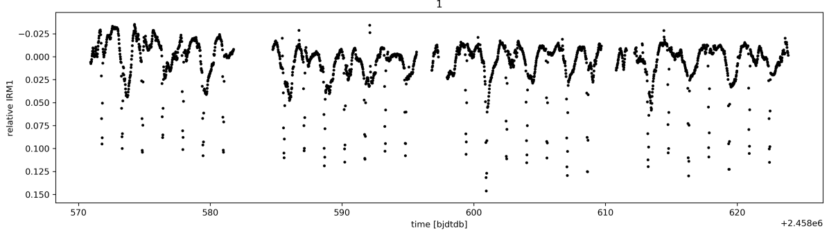
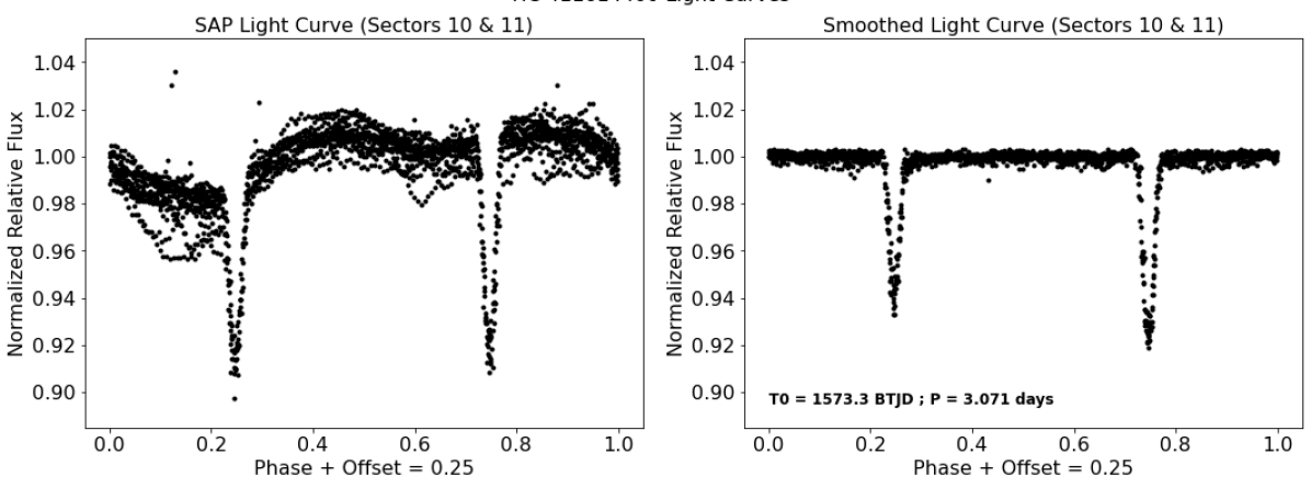
Figure 1: (Top) Discovery light curve of 2M1222$-$57 from TESS FFI observations of sectors 10 and 11 (see Bouma et al., 2019). (Bottom) Light curve phase folded on period of 3.071 d with (right) and without (left) out-of-eclipse variations removed. Note that the out-of-eclipse variations include both a periodic modulation with peak-to-peak amplitude of $\sim$0.075 mag and an additional, more stochastic, source of variability at the level of $\sim$1%.

2 The 2M1222$-$57 Eclipsing Binary System: Variability, Group Membership, Age, and Distance Considerations

2.1 Discovery Light Curve Variability Characteristics

2M1222$-$57 was identified as a likely pre–main-sequence (PMS) eclipsing binary (EB) in TESS light curve data as part of the Cluster Difference Imaging Photometric Survey (CDIPS; see Bouma et al., 2019) of young star-forming regions. Its identifier in the TESS Input Catalog (TIC; Stassun et al., 2019) is TIC 411614400, and the TIC cross-matches it in various other source catalogs as 2MASS J12220147$-$5737565, WISEA J122201.42$-$573756.6, ASAS J122201$-$5737.8, ROSAT 2RXS J122201.0$-$573754, UCAC4 162$-$087608, among others. Its Gaia DR2 identifier is 6071734350857944704. We opt to refer to the object by its shorthand 2MASS identifier: 2M1222$-$57.

The CDIPS light curve from the Full Frame Images (FFIs; see, e.g., Oelkers & Stassun, 2018) in TESS observing sectors 10 and 11 (Figure 1, top) exhibited clearly repeating, punctuated flux dropouts with depths of $\sim$0.15 mag superposed on a periodic modulation with peak-to-peak amplitude of $\sim$0.075 mag. The periodic modulation appears to have roughly the same period as the flux dropouts, but the shape of the modulation varies somewhat from cycle to cycle (Figure 1, bottom left), suggesting the presence of some additional source of variability at the level of $\sim$1% amplitude that is more stochastic in nature. There were also a few possible flaring events observed. Applying a simple spline fit to the out-of-eclipse variations reveals a clearly well detached EB light curve with period of 3.071 d (Figure 1, bottom right). The primary and secondary eclipses are separated by 0.5 phase and have depths of $\sim$8% and $\sim$6%, respectively, suggesting a circular orbit and a grazing inclination angle.

2.2 Group Membership, Age, and Distance

2M1222$-$57 has been identified by previous surveys as a PMS star on the basis of the presence of H$\alpha$ emission and very strong Li absorption (see Bowler et al., 2019). In addition, several studies of the spatial and kinematic distributions of young stars in the region have associated 2M1222$-$57 with young moving groups or other coherent, young stellar structures in the solar neighborhood. For example, Kounkel et al. (2020) identify 2M1222$-$57 to be part of the Sco Cen OB association (Figure 2), namely towards Lower Centaurus Crux (LCC).

Using Sagitta, a neural net based algorithm that enables age estimates of PMS stars from their astrometry and photometry (McBride et al., 2021), we derive an age of $\log\tau=7.21\pm 0.06$ ($16.2\pm 2.2$ Myr). This is consistent with the age of $\sim$16 Myr inferred for LCC by several other studies (see, e.g., Preibisch & Mamajek, 2008, and references therein).

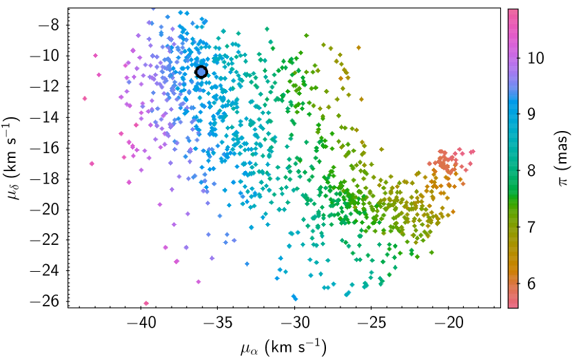
Figure 2: Spatial map of LCC and its proper motions (from McBride et al., 2021) color-coded by the inferred age and parallax respectively. 2M1222$-$57  is highlighted against LCC with a larger circle with black outline.

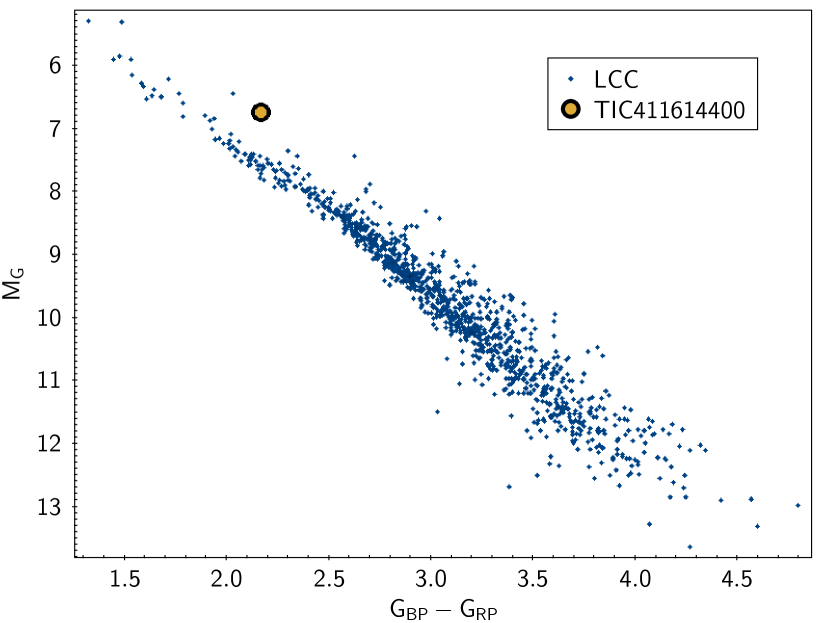
Figure 3: Gaia color-magnitude diagram of LCC (from McBride et al., 2021) in black, and 2M1222$-$57 marked by the yellow circle.

2M1222$-$57 stands out among the other members of LCC, its position in the color-magnitude diagram distinguishing it as one of the most luminous objects for its color (Figure 3). This is attributable to its placement on the cluster binary sequence rather than being younger than its siblings: Bowler et al. (2019) identify it as a likely spectroscopic binary with spectral type of approximately M1. The Gaia reported RUWE value of 1.5 is also consistent with the presence of photocenter motion as would be expected for a binary with stars of near-equal brightness (see, e.g., Stassun & Torres, 2021).

Finally, the Gaia DR3 parallax measurement of $9.453\pm 0.025$ mas (including the most recent published global parallax offset and inflation factor on the parallax uncertainty; see Lindegren et al., 2021; El-Badry et al., 2021) securely places 2M1222$-$57 at a distance of $105.79\pm 0.28$ pc. As we will see below, this precise distance measurement helps us place stringent constraints on the temperatures and radii of the eclipsing stellar components of the 2M1222$-$57 system.

3 Data

3.1 TESS Light Curve

TESS observed 2M1222$-$57 in its 30-min FFI mode over nearly 60 d in Sectors 10–11, and again in its 2-min mode over another nearly 60 d in Sectors 37–38 (Figures 1, 4–5). The latter observations were through the Director’s Discretionary Target program (PI: Bouma).

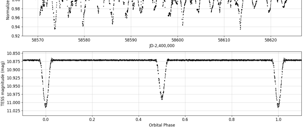
Figure 4: Phase-folded TESS FFI light curve from Sectors 10–11 (Figure 1) after smoothing out the out-of-eclipse variations.

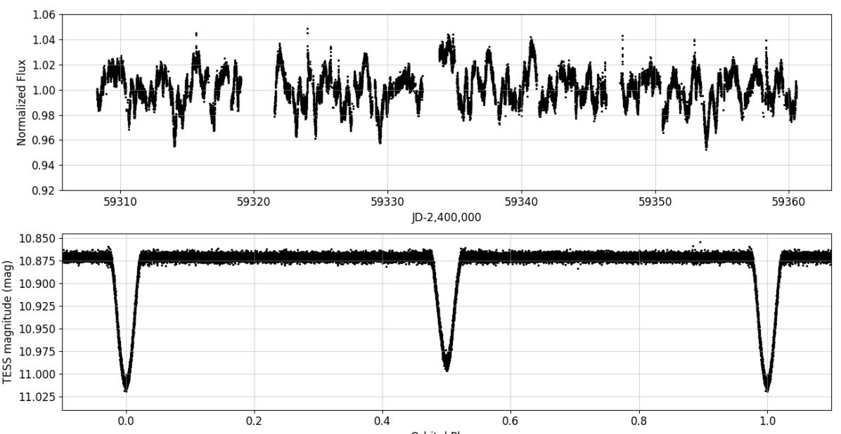
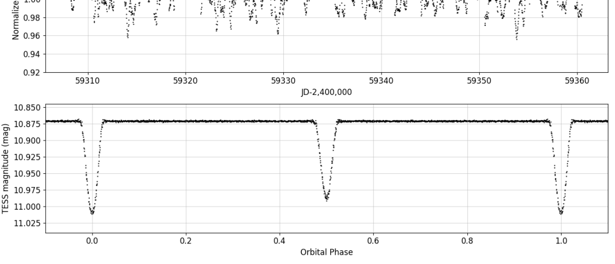
Figure 5: TESS 2-min cadence light curve from Sectors 37–38. (Top) Points in eclipse have been removed to isolate the out-of-eclipse variations. (Middle) Phase-folded on the orbital period after smoothing out the out-of-eclipse variations. (Bottom) Same as middle, but binned by 30 min for comparison with Sectors 10–11 (Figure 4).

Unfortunately there is no flux contamination estimate provided by the TIC because this star was not selected for inclusion in the TESS Candidate Target List (CTL; Stassun et al., 2019). Therefore, we constructed custom pixel masks to extract the TESS light curve from each sector based on a careful assessment of all surrounding stars included in the TIC (Figure 6). In addition, we used the apparent TESS magnitudes of all stars in the TIC that could contribute flux within the pixel masks in order to correct for dilution of the eclipses and other variations. We obtain flux contamination fractions (flux of contaminants relative to total flux) of 0.301, 0.276, 0.307, and 0.318, for Sectors 10, 11, 37, and 38, respectively.

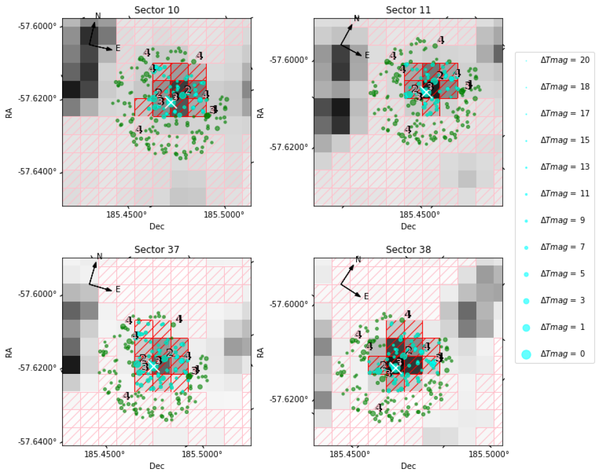
Figure 6: Cutouts of Full Frame Images from TESS Sectors 10–11, and of 2-min observations from TESS Sectors 37–38, centered on 2M1222$-$57. Other stars from the TIC within (cyan) and outside of (green) the pixel mask are shown along with their apparent TESS magnitudes.

The light curve also exhibits out-of-eclipse variations with peak-to-peak amplitude of $\sim$5%, which include a combination of instrumental systematics and true source modulations. As shown in Figure 1, the modulations change significantly from cycle to cycle, which complicates the analysis with an EB model. We therefore opted to detrend the light curve manually, by masking out the eclipses and fitting a cubic spline function to the out-of-eclipse portions in order to remove the variability. We did this separately for the data with 30 m and 2 m cadence, and modeled both the periodic component (more clearly seen in sectors 10–11) and the more stochastic component that seems to dominate in sectors 37–38. In each case we set the smoothing factor $s$ (see footnote 1) that controls the number of spline knots to provide a reasonable approximation as assessed visually, while at the same time avoiding overfitting of noise as well as undue variations in the masked-out eclipse sections that might affect the shape of the underlying eclipses. We then divided the raw light curve by these spline functions, interpolating over the eclipse sections. This is the final photometry that we will use below in Section 4.2. The phase-folded light curves for sectors 10–11 and 37–38 are shown in the bottom panels of Figures 4 and 5.

3.2 Radial Velocities

2M1222$-$57 was observed at 17 separate epochs with the CHIRON echelle spectrograph on the CTIO 0.9-m telescope from 29 Jan 2021 to 28 Apr 2021 in the fiber mode configuration ($R\approx$ 25,000, $\lambda\lambda$410–870 nm). At most epochs, the observed spectrum was clearly double-lined and the relative line strengths suggested components of similar brightness. For example, Figure 7 shows the observed spectrum at one representative epoch for the regions around the Li $\lambda$6708 line and the H$\alpha$ $\lambda$6563 line. One epoch had the two components severely blended, making it difficult to obtain accurate radial velocities; this spectrum was therefore not used for our analysis.

We extracted radial velocities (RV) for both components using the Python implementation of the IRAF XCSAO function (Kurtz & Mink, 1998; Kounkel, 2022), through performing a cross-correlation against a high resolution PHOENIX synthetic spectrum (Husser et al., 2013) with solar metallicity, $T_{\rm eff}=3600$ K, and $\log g$=4.0. To minimize the noise from the joining of the echelle orders, to avoid H$\alpha$ emission line that is not represented in the template, as well as to avoid strong telluric features and maximize the RV precision, cross-correlation was done only using the wavelength range of 7000–8000 Å, and a Fourier filter was applied to minimize low spatial frequencies. Across all epochs, the cross-correlation function showed two strongly pronounced peaks, velocities of which were obtained independently through Gaussian fitting. The RVs so measured are summarized in Table 3.2.

Table 1: Radial Velocities of 2M1222$-$57

BJD	RV1	$\sigma_{\rm RV_{1}}$	RV2	$\sigma_{\rm RV_{2}}$
	km s-1	km s-1	km s-1	km s-1
2459243.81852	88.46	0.34	$-$68.55	0.62
2459245.73937	$-$25.38	0.53	56.56	0.69
2459249.83554	90.93	0.34	$-$72.40	0.66
2459250.83505	$-$22.03	0.50	51.59	0.72
2459251.76984	$-$41.21	0.49	73.91	0.62
2459263.79932	$-$60.56	0.40	93.92	0.48
2459264.79986	67.57	0.54	$-$46.83	0.64
2459266.76239	$-$64.19	0.42	97.27	0.48
2459266.77633	$-$64.09	0.37	96.58	0.47
2459272.71189	$-$60.26	0.39	93.33	0.50
2459274.72963	76.10	0.43	$-$55.21	0.53
2459278.80614	$-$57.11	0.45	90.34	0.49
2459329.59451	87.87	0.39	$-$69.73	0.44
2459329.73206	89.54	0.40	$-$73.18	0.47
2459331.62970	$-$39.00	0.70	70.73	0.95
2459332.59585	84.98	0.41	$-$68.22	0.46

In addition, from this analysis we measured the secondary-to-primary spectroscopic flux ratio in six different orders unaffected by telluric lines between about 770 nm and 890 nm, spanning the center of the TESS bandpass. The average flux ratio obtained is $0.79\pm 0.05$, which we use below to break the degeneracy between the sum of the stellar radii and the individual radii.

3.3 Lithium and H$\alpha$

As noted above, the spectroscopic observations used to measure the stellar RVs also include the youth indicator Li I at $\lambda$6708 as well as the activity indicator H$\alpha$ at $\lambda$6563. From the epochs where we were able to easily discriminate the two components without blending, we obtain for H$\alpha$ an equivalent width of $-1.5\pm 0.1$ Å and $-1.3\pm 0.1$ Å for the primary and secondary, respectively. For Li we obtain equivalent widths for the primary and secondary, respectively, of $0.30\pm 0.03$ Å and $0.18\pm 0.01$ Å, consistent with the previously reported value of 0.46 Å for the two stars combined (Bowler et al., 2019). Corrected for dilution by the light of the other star (see Section 4.1), we obtain the intrinsic equivalent widths of Li to be $0.53\pm 0.05$ Å and $0.40\pm 0.06$ Å, respectively; for H$\alpha$ we obtain equivalent widths of $-2.6\pm 0.3$ Å and $-3.0\pm 0.3$ Å, respectively.

In addition, from the widths of the Li lines we obtain a measure of the full-width at half-maximum of $0.78\pm 0.05$ Å for both components, corresponding to a projected rotational velocity of $v\sin i=14.7\pm 1.0$ km s^-1. As we will see below, the two eclipsing stars have radii of $\approx$0.95 R_⊙, such that this $v\sin i$ implies a rotation period of $3.27\pm 0.22$ d (assuming $i\approx 90^{\circ}$) for both stars, consistent with synchronous rotation at the orbital period of 3.071 d (see above).

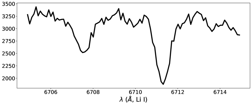
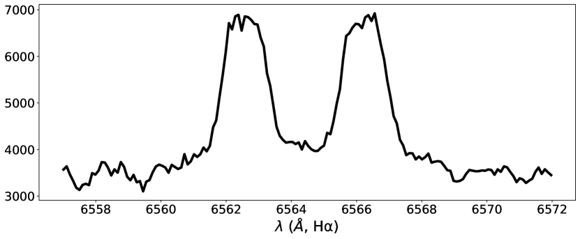
Figure 7: Representative double-line spectrum of 2M1222$-$57 for the region around the Li $\lambda$6708 line (top) and the H$\alpha$ $\lambda$6563 line (bottom).

3.4 Speckle Imaging

High-resolution imaging data was acquired for 2M1222$-$57 with the Zorro speckle instrument on the 8-m Gemini South telescope (Scott et al., 2021) on UT 2022 March 19. Zorro collects speckle imaging observations simultaneously in two bands (562 nm and 832 nm) with integration times of 60 msec per frame. Seven thousand such observations are obtained and reduced as described in Howell et al. (2011), yielding a high-resolution view of the scene near 2M1222$-$57.

Figure 8 shows the resulting 5-$\sigma$ contrast curves obtained in each filter and the reconstructed speckle image in 832 nm. An angularly close stellar companion to 2M1222$-$57 was discovered in the 832 nm image residing 0$\farcs$89 away at PA = 333.66^∘. The companion star is $3.3\pm 0.3$ magnitudes fainter than the central EB, and was not reported in any known point source catalogs, including Gaia DR3.

No other close companions were detected to within a contrast of 5–8 magnitudes for separations ranging from the diffraction limit ($\sim$20 mas) to 1$\farcs$2.

4 Analysis and Results

4.1 Spectral Energy Distribution: Initial Constraints on Stellar Properties

In order to obtain initial estimates of the component effective temperatures ($T_{\rm eff}$) and radii ($R$), we performed a multi-component fit to the combined-light, broadband SED of the 2M1222$-$57 system, including broadband photometry from Gaia DR3, 2MASS, and WISE (see Stassun & Torres, 2016; Miller et al., 2020, for details of the SED fitting methodology specifically in the context of EBs).

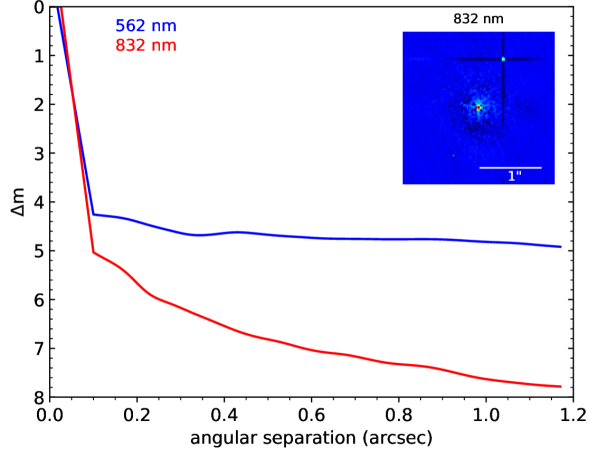
Figure 8: Speckle imaging at 832 nm of 2M1222$-$57 showing the presence of a faint tertiary companion with $\Delta m=3.3\pm 0.3$ at a separation of 0$\farcs$89 (i.e., $\sim$100 AU physical separation).

We started by treating the SED as a single star with $T_{\rm eff}$ estimate based on the spectral type of M1 reported from the spectroscopic observations of Bowler et al. (2019). We then redid the fit using two stellar photospheres, their individual $T_{\rm eff}$ and $R$ informed by the eclipse modeling and the total system flux enforced to be consistent with the tight Gaia distance constraint (see Section 2.2), and then also including the small contribution of light from the faint tertiary companion observed in the speckle imaging (see Section 3.4). The resulting $T_{\rm eff}$ and $R$ were iteratively updated based on the joint light-curve and radial-velocity model (Section 4.2) until a final satisfactory SED fit was produced.

As shown in Figure 9 (black curve), the SED from 0.4 $\mu$m to 4 $\mu$m can be very well fit by a single component with $T_{\rm eff}=3660\pm 100$ K (corresponding to spectral type M1$\pm$1; Bowler et al., 2019), $\log g\approx 4.3$, [Fe/H]$\,\approx\,$0, and extinction of $A_{V}\approx 0$ (consistent with other determinations of the reddening to this region; e.g., Kounkel et al., 2020). The WISE photometry at 10 $\mu$m and 22 $\mu$m shows what appears to be an excess, which we later model in the context of a circumbinary disk, but which we exclude from the SED fitting at this stage.

The single-star fit suggests that the two eclipsing components have $T_{\rm eff}$ comparable to one another and close to 3660 K. This is reinforced by the similarity of the primary and secondary eclipses in the TESS light curve, and by the similarity of the strengths of the Li absorption line, though the fact that they are not identical clearly indicates that the two components must have slightly different $T_{\rm eff}$. In fact, the relative eclipse depths imply the ratio of stellar surface brightnesses in the TESS bandpass to be $0.853\pm 0.002$ (see Section 4.2), which provides a constraint on the ratio of $T_{\rm eff}$ from the model atmospheres.

An additional constraint is provided by the eclipse durations, which very tightly constrain the sum of the radii of the eclipsing bodies to be $R_{\rm sum}=1.918\pm 0.010$ R_⊙ (see Section 4.2). Another constraint is provided by the ratio of fluxes of the two stars from their relative line strengths in the spectra used to measure the radial velocities (Section 3.2), which give $F_{2}/F_{1}=0.79\pm 0.05$ at $\sim$830 nm, averaged over all epochs. Finally, the combined bolometric luminosities of the two stars via the Stefan-Boltzmann relation must reproduce the observed combined-light bolometric flux at Earth given the precise distance provided by Gaia.

A final iteration was required to self-consistently incorporate the small flux contribution of the tertiary companion (magenta curve in Figure 9). The one direct constraint is provided by the contrast ratio measured in the speckle imaging of the companion relative to the combined light of the EB (Section 3.4), represented in Figure 9 by the flux measurement at 832 nm fitted by the magenta curve. For the companion we assumed $T_{\rm eff}=3230$ K and $R=0.47$ R_⊙ (corresponding to a mass of $\approx$0.18 M_⊙), guided by the predictions of the Baraffe et al. (2015) PMS evolutionary models for the nominal 16.2 Myr age of the system (see Section 2.2). In our best-fit SED model, the tertiary companion contributes 4.5% of the total light relative to that of the EB, consistent with the estimate of $2.0^{+3.2}_{-1.4}$% “third light” ($l_{3}$) in the eclipse light curve model (Section 4.2).

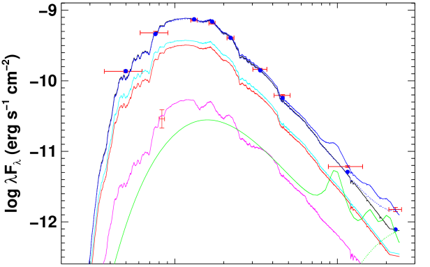
Figure 9: Multi-component fit to the combined-light SED of 2M1222$-$57 with NextGen stellar atmosphere models. Observed fluxes are represented as red symbols (horizontal error bars represent filter widths); blue symbols are the corresponding model fluxes. The black curve is a single-source fit using $T_{\rm eff}=3660$ K, [Fe/H]=0, and $A_{V}=0$, based on the spectroscopic observations of Bowler et al. (2019). Final multi-component fit includes contributions from the primary eclipsing star (cyan curve), the secondary eclipsing star (red curve), the tertiary companion (magenta curve), and the circumbinary disk (green curve). The disk component is represented both without any material within the central cavity (dotted curve) and with $8\times 10^{-10}$ M_⊙ (i.e., $3\times 10^{-4}$ M_⊕) of optically thin dust within the cavity (solid curve). The dark blue curve represents the sum total of all components (dotted and solid for the disk model without and with material in the cavity, respectively). Residuals at bottom are in $\sigma$ units, in the sense of $(O-C)/\sigma_{o}$ for both the bare stellar model (black) and the full multi-component model (blue).

The resulting best-fit SEDs for the two eclipsing stars are represented in Figure 9 by the cyan and red curves, respectively, with best-fit $T_{\rm eff}$ of 3749$\pm$35$\pm$11 K and 3645$\pm$35$\pm$11 K, respectively (we adopt an 11 K systematic error for this methodology; see Miller et al., 2020), best-fit $R$ of 0.981$\pm$0.018 R_⊙ and 0.957$\pm$0.016 R_⊙, respectively, and $A_{V}=0.00^{+0.05}_{-0.00}$. These parameters successfully reproduce the $R_{\rm sum}$ constraint (1.937$\pm$0.019 R_⊙ versus 1.918$\pm$0.010 R_⊙ from the final eclipse model; see Section 4.2), the spectroscopic flux ratio constraint (0.82$\pm$0.04 versus 0.79$\pm$0.05 from the spectra), the surface brightness ratio constraint (0.851$\pm$0.002 versus 0.853$\pm$0.002 from the average of the 30-min and 2-min cadence light curves in the final eclipse model), and the Gaia distance (105.63$\pm$0.29 pc versus 105.79$\pm$0.28 pc).

The final physical parameters and their precise uncertainty estimates that we ultimately adopt are those provided by the joint MCMC modeling of the eclipse light curves and the radial-velocity measurements described below (Section 4.2). However, the success of those parameters in reproducing the SED and its various hard constraints is a very strong validation of the global solution for the 2M1222$-$57 system, which we now discuss.

4.2 TESS Light Curve Analysis: Determination of Stellar Properties

We analyzed the TESS light curves of 2M1222$-$57 using the Nelson-Davis-Etzel binary model (Etzel, 1981; Popper & Etzel, 1981), as implemented in the eb code of Irwin et al. (2011). This model is appropriate for well-detached systems such as this in which the stars are essentially spherical (see below), and the eb code facilitates its use within a Markov chain Monte Carlo (MCMC) environment. The 30 m and 2 m photometry was analyzed jointly with the radial velocities.

We considered the following adjustable light curve parameters: the orbital period ($P$), a reference time of primary eclipse ($T_{0}$), the central surface brightness ratio in the TESS band ($J\equiv J_{2}/J_{1}$), the sum of the relative radii normalized by the semimajor axis ($r_{1}+r_{2}$), the radius ratio ($k\equiv r_{2}/r_{1}$), the cosine of the orbital inclination angle ($\cos i$), an out-of-eclipse brightness level in magnitude units ($m_{0}$), and the eccentricity parameters $\sqrt{e}\cos\omega_{1}$ and $\sqrt{e}\sin\omega_{1}$, where $e$ is the eccentricity and $\omega_{1}$ the argument of periastron for the primary. In view of the noticeable and irregular distortions in the light curve, we chose to adopt a linear limb-darkening law and allowed the coefficients ($u_{1}$, $u_{2}$) to vary freely; tests with a quadratic law yielded no improvement, and did not change the geometric quantities. In addition to the above, the discovery of a close companion to 2M1222$-$57 described later prompted us to include an additional parameter, $\ell_{3}$, to account for third light. It is defined such that $\ell_{1}+\ell_{2}+\ell_{3}=1$, in which $\ell_{1}$ and $\ell_{2}$ for this normalization are taken to be the light at first quadrature. The spectroscopic parameters in our analysis were the primary and secondary velocity semiamplitudes ($K_{1}$ and $K_{2}$), and the center-of-mass velocity ($\gamma$).

Because the detrending of the photometry was done independently for the 30 m and 2 m data, as a precaution we allowed separate values of $J$ and $m_{0}$ to account for possible differences introduced during that process, as well as the possibility of errors in the contamination corrections. The normalization of these light curves described in Section 3.1 artificially removes any variations out of eclipse. Consequently, gravity darkening and reflection become irrelevant. For consistency, we therefore used the option in the eb code that suppresses those effects in calculating the binary model. Furthermore, as the (flattened) out-of-eclipse portions of the light curve contain no additional information, we retained only segments within 0.075 in phase units from the center of each eclipse, equivalent to about one and a half times the total eclipse duration.

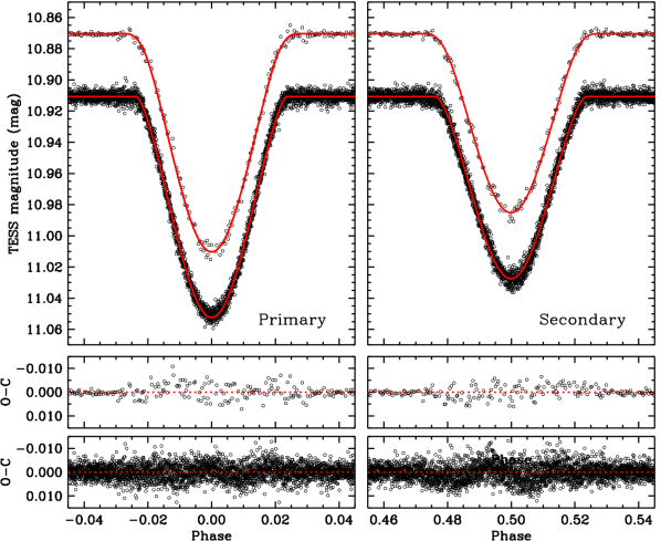
Figure 10: Detrended TESS observations of 2M1222$-$57 (2 m and 30 m cadence) at primary and secondary eclipse. The 30 m data are displaced vertically for clarity, the solid curve is our binary model. Residuals for both data sets are shown at bottom.

Observational uncertainties were handled by including four additional free parameters representing multiplicative scale factors for the internal observational errors in each of the data sets: the 30 m and 2 m photometry, and the primary and secondary RVs. The internal errors for the RVs are those given in Table 3.2, and for the 30 m and 2 m photometry we adopted values of 0.002 and 0.003 mag, respectively. These four additional parameters were solved simultaneously and self-consistently with the other variables (see, e.g., Gregory, 2005).

We carried out our joint lightcurve and RV analysis using the emcee code of Foreman-Mackey et al. (2013), which is a Python implementation of the affine-invariant MCMC ensemble sampler proposed by Goodman & Weare (2010). We used 100 walkers with chain lengths of 20,000 each, after discarding the burn-in. All parameters used uniform or log-uniform priors over suitable ranges that are listed in the last column of Table 2. We verified convergence by visual examination of the chains, and requiring a Gelman-Rubin statistic of 1.05 or smaller for each parameter (Gelman & Rubin, 1992). The cadence of the TESS FFIs (30 m) corresponds to a fraction of the 3.07 day orbital period of 2M1222$-$57 that is not quite negligible, equivalent to about 0.007 in phase units. To avoid biases from smearing, we oversampled the model light curve at each iteration of our solution, and then integrated over the 30 m duration of each cadence prior to the comparison with the observations (see Gilliland et al., 2010; Kipping, 2010).

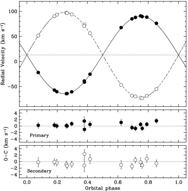
Figure 11: Radial-velocity measurements of 2M1222$-$57 with our adopted model. Primary and secondary observations are represented with filled and open circles, respectively, the dotted line marks the center-of-mass velocity of the system. Error bars are smaller than the symbol sizes. Residuals are shown at bottom.

Initial solutions revealed that the radius ratio $k$ was poorly constrained by the photometry. This is often the case in eclipsing binaries such as 2M1222$-$57 with partial eclipses and similar components, and is caused by strong correlations with other free parameters. For example, in our case the correlation coefficient between $k$ and $\cos i$ was $-0.989$, and between $k$ and $r_{1}+r_{2}$ it was $-0.984$. A common remedy is to require the lightcurve solution to be consistent with an independently measured light ratio, such as from spectroscopy (see, e.g., Andersen et al., 1980). This is effective because the light ratio depends very strongly on the radius ratio: $\ell_{2}/\ell_{1}\propto k^{2}$. We therefore applied our flux ratio from CHIRON ($0.79\pm 0.05$, measured at wavelengths near the center of the TESS bandpass) as a Gaussian prior, and this largely removed the degeneracy.

It was also noticed that the residuals of the primary velocities were predominantly positive, and those of the secondary mostly negative. We speculate that this unphysical effect may be a consequence of distortions in the spectral line profiles produced by spots, which can then affect the velocities. For our final solution we chose to solve for separate values of $\gamma$ for each component, which removed the bias.

Table 2: Joint Photometric-Spectroscopic Solution for 2M1222$-$57

Parameter	Value	Prior
$P$ (days)	$3.07165752^{+0.00000034}_{-0.00000033}$	[3.0, 3.1]
$T_{0}$	$571.768221^{+0.000080}_{-0.000081}$	[571.7, 572.0]
$J$, 30 m data	$0.951^{+0.039}_{-0.017}$	[0.4, 1.2]
$J$, 2 m data	$0.955^{+0.039}_{-0.017}$	[0.4, 1.2]
$r_{1}+r_{2}$	$0.19295^{+0.00078}_{-0.00167}$	[0.01, 0.40]
$k\equiv r_{2}/r_{1}$	$0.966^{+0.021}_{-0.023}$	[0.5, 2.0]
$\cos i$	$0.1258^{+0.0011}_{-0.0025}$	[0, 1]
$\sqrt{e}\cos\omega_{1}$	$-0.0049^{+0.0023}_{-0.0063}$	[$-$1, 1]
$\sqrt{e}\sin\omega_{1}$	$+0.033^{+0.037}_{-0.045}$	[$-$1, 1]
$u_{1}$	$0.121^{+0.051}_{-0.057}$	[0.0, 1.0]
$u_{2}$	$0.429^{+0.037}_{-0.040}$	[0.0, 1.0]
$m_{\rm 0,\,30min}$ (mag)	$10.870415^{+0.000083}_{-0.000082}$	[10, 11]
$m_{\rm 0,\,2min}$ (mag)	$10.870696^{+0.000035}_{-0.000034}$	[10, 11]
$\ell_{3}$	$0.020^{+0.032}_{-0.014}$	[0.0, 0.5]
$\gamma_{1}$ (km s-1)	$+13.18^{+0.19}_{-0.19}$	[0, 20 ]
$\gamma_{2}$ (km s-1)	$+12.63^{+0.27}_{-0.27}$	[0, 20 ]
$K_{1}$ (km s-1)	$77.44^{+0.21}_{-0.21}$	[50, 100 ]
$K_{2}$ (km s-1)	$85.26^{+0.30}_{-0.30}$	[50, 100 ]
$f_{\rm 30\,m}$	$1.005^{+0.030}_{-0.028}$	[$-$5, 5]
$f_{\rm 2\,m}$	$0.9944^{+0.0069}_{-0.0069}$	[$-$5, 5]
$f_{\rm RV1}$	$1.73^{+0.45}_{-0.27}$	[$-$5, 5]
$f_{\rm RV2}$	$1.89^{+0.51}_{-0.30}$	[$-$5, 5]
Derived quantities
$r_{1}$	$0.0980^{+0.0012}_{-0.0012}$	$\cdots$
$r_{2}$	$0.0946^{+0.0012}_{-0.0015}$	$\cdots$
$i$ (degree)	$82.773^{+0.146}_{-0.061}$	$\cdots$
$e$	$0.0012^{+0.0037}_{-0.0010}$	$\cdots$
$\ell_{2}/\ell_{1}$, 30 m data	$0.798^{+0.035}_{-0.035}$	$G(0.79,0.05)$
$\ell_{2}/\ell_{1}$, 2 m data	$0.801^{+0.035}_{-0.035}$	$G(0.79,0.05)$
$J_{\rm ave}$, 30 m data	$0.852^{+0.021}_{-0.008}$	$\cdots$
$J_{\rm ave}$, 2 m data	$0.855^{+0.021}_{-0.006}$	$\cdots$

Note. — Values correspond to the mode of the posterior distributions, uncertainties represent 68.3% credible intervals. Priors in square brackets are uniform over the specified ranges, except the ones for $f_{\rm 30\,m}$, $f_{\rm 2\,m}$, $f_{\rm RV1}$ and $f_{\rm RV1}$, which are log-uniform, and the ones for the light ratios, which are Gaussian, indicated as $G({\rm mean},\sigma)$.

Table 2 presents the results of the analysis. We list the mode of the posterior distribution for each parameter, along with the corresponding 68.3% credible intervals. The posterior distributions for the derived quantities in the bottom section of the table were constructed directly from the MCMC chains of the adjustable parameters involved. The eccentricity of the orbit is not statistically significant. We derive a 3$\sigma$ upper limit of $e\approx 0.01$. The oblateness indices for the stars, calculated following the prescription by Binnendijk (1960), are 0.0013 for the primary and 0.0014 for the secondary. These are well below the upper limit of 0.04 considered safe for the Nelson-Davis-Etzel binary model (see, e.g., Popper & Etzel, 1981), justifying its use. The photometric observations are shown together with our model in Figure 10. The corresponding graphic for the radial velocities is presented in Figure 11.

Our mass and radius determinations for 2M1222$-$57 are among the best determined for PMS stars. The masses have relative precisions of 0.8 and 0.7% for the primary and secondary, and the absolute radii are determined to 1.3% and 1.6%, respectively. We list these results in Table 3 along with other derived properties. The bolometric luminosities listed in the table are from the Stefan-Boltzmann relation, based on these radii together with the effective temperatures as determined from the SED fit (see Section 4.1).

As a sanity check, the distance to the system may be calculated directly (and independently from Gaia) from the luminosities, the apparent visual magnitude ($V=11.468\pm 0.087$; Kiraga, 2012), and bolometric corrections $BC_{\rm V}$ of $-1.30$ and $-1.44$ for the primary and secondary, respectively, based on the work of Eker et al. (2020). The extinction is negligible according to our SED fit ($A_{\rm V}<0.05$).

The value we obtain, $104.7\pm 9.8$ pc, corresponds to a parallax of $9.49\pm 0.89$ mas which, although much less precise than the determination from Gaia DR3 ($9.453\pm 0.025$ mas; see Table 3) is in good agreement with it. The large error in the distance in this calculation is driven by the errors in $V$ (affected by the intrinsic variability), the bolometric corrections, and the adopted uncertainty in the interstellar extinction.

Finally, on the assumption of spin-orbit synchronization and alignment, the predicted rotational velocities are near 16 km s^-1 for both stars. This is fairly close to our spectroscopic determination (Section 3.2).

4.3 Photometric Variability

As noted in Section 3.1, the TESS light curve of 2M1222$-$57 exhibits variability beyond the primary and secondary eclipses, at a level of $\sim$5% peak to peak. We attempted to characterize these variations in the context of rotationally modulated spot variations on one or more of the stars in the system, as such spot-driven variations at levels of a few percent to nearly 50% peak-to-peak are frequently observed among low-mass PMS stars (see, e.g., Stassun et al., 1999, for examples).

Table 3: Physical Properties of 2M1222$-$57

Parameter	Primary	Secondary
$M$ ($\mathcal{M}_{\sun}^{\rm N}$)	$0.7354\pm 0.0057$	$0.6680\pm 0.0044$
$R$ ($\mathcal{R}_{\sun}^{\rm N}$)	$0.976\pm 0.013$	$0.942\pm 0.015$
$\log g$ (dex)	$4.33\pm 0.011$	$4.31\pm 0.013$
$q\equiv M_{2}/M_{1}$	$0.9083\pm 0.0041$
$a$ ($\mathcal{R}_{\sun}^{\rm N}$)	$9.956\pm 0.023$
$T_{\rm eff}$ (K)	$3749\pm 35$	$3645\pm 35$
$L$ ($L_{\sun}$)	$0.169\pm 0.008$	$0.141\pm 0.007$
$M_{\rm bol}$ (mag)	$6.67\pm 0.05$	$6.87\pm 0.05$
$BC_{V}$ (mag)	$-1.30\pm 0.21$	$-1.44\pm 0.21$
$M_{V}$ (mag)	$7.97\pm 0.22$	$8.31\pm 0.22$
$v_{\rm sync}\sin i$ (km s-1)	$15.94\pm 0.21$	$15.40\pm 0.24$
$v\sin i$ (km s-1)	$14.7\pm 1.0$	$14.7\pm 1.0$
$E(B-V)$ (mag)	$<0.02$
$A_{V}$ (mag)	$<0.05$
$\pi_{Gaia/{\rm DR3}}$ (mas)	$9.453\pm 0.025$
$d_{Gaia/{\rm DR3}}$ (pc)	$105.79\pm 0.28$

Note. — The masses, radii, and semimajor axis $a$ are expressed in units of the nominal solar mass and radius ($\mathcal{M}_{\sun}^{\rm N}$, $\mathcal{R}_{\sun}^{\rm N}$) as recommended by 2015 IAU Resolution B3 (see Prša et al., 2016), and the adopted solar temperature is 5772 K (2015 IAU Resolution B2). Bolometric corrections are from the work of Eker et al. (2020). See text for the source of the reddening. For the apparent visual magnitude of 2M1222$-$57 out of eclipse we used $V=11.468\pm 0.087$ (Kiraga, 2012).

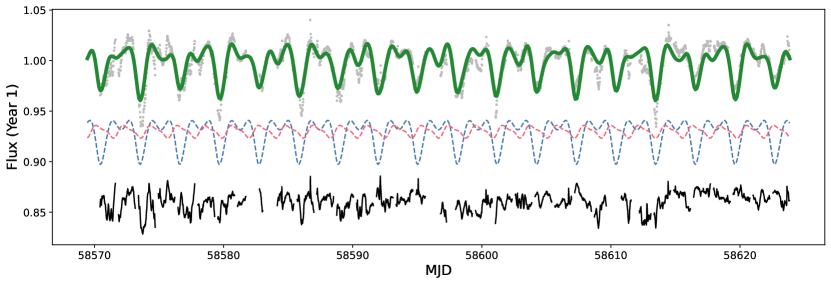
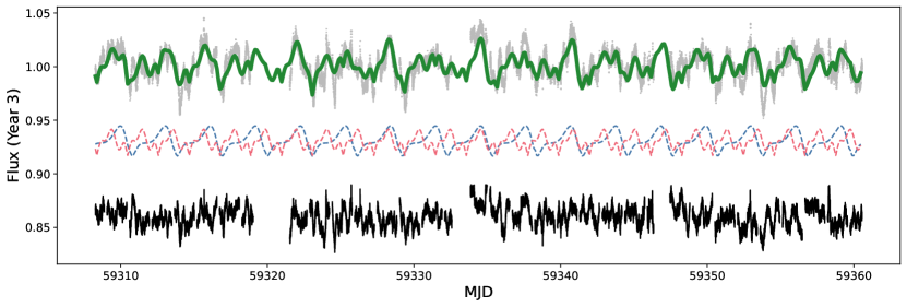
Figure 12: Out-of-eclipse variations in the TESS light curve of 2M1222$-$57 for Sectors 10–11 (top) and Sectors 37–38 (bottom). While there is some change in overall morphology of the variations, at both epochs the variations can be characterized with two dominant periodic components: a “double-humped” component at the orbital period that we attribute to rotationally modulated spot variations on one or both of the eclipsing stars (blue dashed curve) and a somewhat more complex, sawtooth-like component with a period of 2.1 d that we attribute to rotationally modulated spot variations on the tertiary companion (red dashed curve). Both periodic components added together are shown in green overlaid on the TESS light curve data (grey symbols). The residuals (black, bottom) reveal additional, quasi-stochastic variations at the level of $\sim$2% peak-to-peak that may be attributable to accretion in the system from the circumbinary disk (see Section 5).

To model this variability, we first removed all the fluxes corresponding to the eclipses. We then folded the light curve to the dominant period found with a Lomb-Scargle periodogram, which was the same as the orbital period, or $\sim$3.07 d. We then fitted an 8th degree polynomial to this folded light curve and subtracted it out. This was done independently to the Year 1 data corresponding to Sectors 10–11, and Year 3 data corresponding to Sectors 37–38.

Significant variability remained in the residuals, showing a secondary periodic signature, with a period of $\sim$2.1 d, consistent both in Year 1 and Year 3. It was similarly fit with an 8th degree polynomial in the newly folded residual light curve, independently in Year 1 and Year 3 data. The resulting fit is shown in Figure 12.

There was some change in overall morphology of the variations during the 2 years that elapsed between TESS Sectors 10–11 and Sectors 37–38, with Year 1 data having a larger amplitude of variability by almost a factor of 2 compared to Year 3 data. Additionally, the Year 1 data show a “simpler” morphology, with fewer harmonic oscillations compared to Year 3. Nonetheless, in both time ranges, the primary period component appears to be “double-humped”, and the secondary component at a period of 2.1 d shows a sawtooth-like morphology.

Adding the two periodic signatures does not fully model the variability. The residuals reveal additional, quasi-stochastic “dip-like” variations at the level of $\sim$2% peak-to-peak. While they are aperiodic, they appear to have a typical duration of $\sim$0.3 d.

We may attribute the periodic components of the variability to rotational modulation of spots on the stars in the system. That one of the periodic components shares the orbital period of the eclipsing stars strongly suggests that it can be ascribed to one or both of the eclipsing stars, whose rotational periods are synchronized with the orbit. The fact that this component appears double-humped could mean either that this signal arises from spots on roughly opposite hemispheres on one of the stars, or that it arises from spots on both stars at roughly opposite longitudes. The observed peak-to-peak amplitude of $\sim$5% implies that the intrinsic amplitude is either $\sim$5% for both stars or $\sim$10% if it arises from one star and diluted by the light of the other.

The second periodic signal cannot readily be attributed to the eclipsing stars. The observed period of 2.1 d is not an obvious harmonic or alias of the orbital period. The more likely source is rotationally modulated spot variations on the tertiary companion. In that case, the observed amplitude of $\sim$1% implies an intrinsic amplitude of $\sim$20%, given the tertiary’s light is diluted by a factor of $\sim$20 by the eclipsing stars.

Finally, the residual quasi-stochastic variations may be attributable to activity or accretion in the system. We defer discussion of this possibility to Section 5.2.

5 Discussion

5.1 Comparison with Stellar Evolution Models

Our precise mass, radius, and temperature determinations offer an opportunity to compare the measurements against current models of stellar evolution for young objects. Figure 13 shows our determinations for the primary and secondary against standard model isochrones from Baraffe et al. (2015) and from the Dartmouth series (Dotter et al., 2008; Feiden, 2016). The best fit age based on our measured radii and masses is near 12 Myr for both sets of models (top panel). However, the effective temperatures appear too cool at these masses (bottom panel), deviating from theoretical predictions by about 5$\sigma$.

As mentioned earlier, stellar activity has been found to affect the global properties of stars with convective envelopes (see, e.g., the reviews by Torres, 2013; Feiden, 2015), often causing them to have larger radii and cooler temperatures than models indicate. One explanation invokes magnetic fields, which are commonly associated with activity and inhibit the convective flow of energy, to which stars respond by increasing their surface area and lowering their temperature. Non-standard models that incorporate magnetic fields have been successful in explaining radius inflation and temperature suppression in several eclipsing main-sequence systems with well measured properties (see, e.g., Feiden & Chaboyer, 2013; MacDonald & Mullan, 2014), and similar models have also been explored for the far fewer eclipsing PMS binaries that have sufficiently precise determinations of their masses, radii, and temperatures (see, e.g., Stassun et al., 2014).

Figure 14 compares the measured properties of 2M1222$-$57 against magnetic models by Feiden (2016), which are an evolution of the same Dartmouth models shown in Figure 13 in which the internal structure equations have been modified to account for magnetic pressure. In this case the age that matches the measured radii of 2M1222$-$57 is somewhat older than before ($17.0\pm 0.5$ Myr), but in better agreement with the age estimated for the LCC association (see Section 2.2), and now the same isochrone also reproduces the temperatures of both components within the uncertainties.

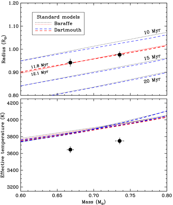
Figure 13: Mass, radius, and effective temperature determinations for the eclipsing binary components of 2M1222$-$57 compared against standard stellar evolution models by Baraffe et al. (2015) and the Dartmouth series (Dotter et al., 2008; Feiden, 2016). Isochrone ages are labeled. The best match to the radii (shown in red) is obtained at about 12 Myr for both models, but theoretical predictions appear too hot at this age.

Figure 14: Same as Figure 13 (and on the same scale), now comparing the measured properties of 2M1222$-$57 against a version of the Dartmouth models that incorporates the effects of magnetic fields (Feiden, 2016). Both the radii and temperatures of the two components are well matched by theory at an age of 17 Myr.

5.2 Activity and Accretion

The TESS light curve of 2M1222$-$57 exhibits quasi-stochastic photometric variability beyond the eclipses and beyond the additional periodic variations that we attribute to spots on the eclipsing stars and the tertiary companion (see Section 4.3). A detailed view of these variations as a function of orbital phase is shown in Figure 15. The variations are complex and exhibit changes in morphology on short timescales. However, there is a recurring “dip” type behavior reminiscent of the persistent and transient flux dips that have now been observed in a large number of young stars (see, e.g., Rebull et al., 2015; Stauffer et al., 2014, 2015, 2017, 2021), of the type which has been attributed in previous studies to transits of the stars by clumps in their protoplanetary disks and/or material in accretion streams.

We also examined the variability of the H$\alpha$ emission lines present in the spectra we used to measure the radial velocities (Section 3.2). Using the spectra from epochs when the two eclipsing stars are well separated in radial velocity, we measured the H$\alpha$ equivalent widths as well as the the full-width at 10% intensity. The former is a commonly used diagnostic for chromospheric activity, the latter has been demonstrated to be a more reliable diagnostic for accretion-related activity specifically (see, e.g., White & Basri, 2003). Both are shown in Figure 16 as a function of orbital phase.

The H$\alpha$ equivalent width variations do not show any clear behavior with orbital phase, and a Lomb-Scargle period search finds no significant periodicity. The H$\alpha$ equivalent widths may therefore be principally a manifestation of the stellar chromospheres which, while exhibiting some degree of true variability, are evidently not sufficiently well organized to produce clear rotationally modulated variations. We return to the implications of the chromospheric activity in Section 5.4.

The H$\alpha$ full widths at 10% intensity, on the other hand, do show evidence for variations on the orbital period. A Lomb-Scargle period search applied to the secondary’s variations independently finds a best period of 3.07 d (i.e., identical to the orbital period) with a false-alarm probability of 0.03. A best-fit sinusoid is represented in Figure 16 to guide the eye, but is not intended to suggest that the variations are in fact sinusoidal. More generically, a Student’s $t$ test applied to the secondary’s measurements on either side of orbital phase 0.5 finds that the means are significantly different with 99.98% confidence.

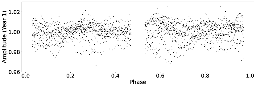
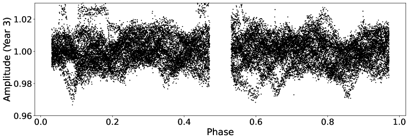
Figure 15: Variability residuals in the TESS light curve data in Sectors 10–11 (top) and Sectors 37–38 (bottom).

A Lomb-Scargle search applied to the primary’s variations in full-width at 10% intensity does not identify any statistically significant periodicity. The primary’s variations do show one measurement near orbital phase 0.4 (i.e., just prior to secondary eclipse) that could be due to a particularly strong accretion event. In addition, a Student’s $t$ test finds, as with the secondary, that the primary’s measurements on either side of orbital phase 0.5 have significantly different means with 99% confidence. Therefore, we again show a best-fit sinusoid on the orbital period in Figure 16 to guide the eye.

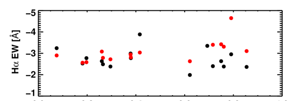
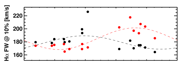
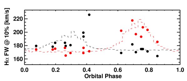
Figure 16: Strength of H$\alpha$ emission as a function of orbital phase for the primary (black symbols) and secondary (red symbols) eclipsing stars. Equivalent width (EW) variations (top) do not exhibit periodic or other clear behavior with orbital phase. Full-width (FW) at 10% intensity variations (middle) of the secondary do exhibit statistically significant periodic behavior, represented by a best-fit sinusoid (red dashed curve); a best-fit sinusoid for the primary (black dashed curve) is also shown for comparison. (Bottom) Same as middle, except curves represent theoretical predictions from the simulations of Artymowicz & Lubow (1996) for the relative accretion rate of circumbinary disk material onto the two stars. The vertical scale for the model curves is arbitrary but the curves have been normalized to preserve the relative accretion rate changes in the model. The black curve representing the model accretion variations for the primary has been shifted by 0.5 phase relative to that for the secondary (red) to simulate the effect of seeing only one longitudinal hemisphere (or “side”) of each star at each orbital quadrature; see the text.

It is interesting that the full-width at 10% intensity variations, assuming they are accretion driven, are aware of the orbital period. Moreover, the times of relatively stronger accretion on the primary and secondary appear to occur near the quadrature phases, when the stars are side by side as seen by the observer, and nearly half an orbital period apart: The best-fit sinusoids in Figure 16 for the primary and secondary peak at phases of $\sim$0.35 and $\sim$0.75, respectively (i.e., separated by $\sim$0.4 in phase). These behaviors are consistent with what has been seen in a few other young binaries that exhibit orbitally pulsed accretion from a circumbinary disk via accretion streams that reach the stars across the hole in the disk carved out by the binary (e.g., Mathieu et al., 1997; Jensen et al., 2007; Ardila et al., 2015).

The canonical examples are DQ Tau (Mathieu et al., 1997; Tofflemire et al., 2017a; Muzerolle et al., 2019), UZ Tau E (Jensen et al., 2007), and TWA 3A (Tofflemire et al., 2017b, 2019). In all cases, the central binary is surrounded by a circumbinary disk whose SED is best modeled by a passive dusty disk with an inner hole that is comparable in size to the binary orbit and that includes a small amount of warm, optically thin dust within the hole. In all cases, photometric variations as well as variations in H$\alpha$ and other spectroscopic accretion indicators (see Ardila et al., 2015) vary periodically with the orbital period in a manner consistent with theoretical predictions (see, e.g., Artymowicz & Lubow, 1996).

In Figure 16 we represent the same model predictions from Artymowicz & Lubow (1996) for the accretion rate variations as a function of orbital phase that were used by Mathieu et al. (1997) for comparison with their observations of DQ Tau. We chose that model because it is the case studied by Artymowicz & Lubow (1996) that has a binary with nearly equal-mass stars, as is the case for the system under consideration here ($q\approx 0.9$; see Table 3). Note, however, that the DQ Tau binary has a considerably longer orbit than 2M1222$-$57 (15.8 d versus 3.07 d) and its orbit is also eccentric. Perhaps most importantly, the DQ Tau binary does not eclipse; in fact, it is likely that it is viewed at a nearly pole-on inclination angle (Basri et al., 1997; Czekala et al., 2016), such that variability arising from accretion stream footpoints on the stellar surfaces may be more easily viewed throughout the orbit. In 2M1222$-$57, only one longitudinal hemisphere (or “side”) of each star can be viewed at each orbital quadrature.

We applied an offset of 0.25 phase to the model accretion rate curves in Figure 16 to match the apparent quadrature phasing of the data. In the model, however, the highest accretion rates onto the two stars occur at the same orbital phase, whereas in 2M1222$-$57 the data imply that the highest accretion rates observed for the primary occur nearly 0.5 phase apart from those observed for the secondary. Therefore, we applied an additional offset of 0.5 phase to the model curve for the primary’s accretion rate in Figure 16. The qualitative agreement between the model and the data suggests that our adjustments to the model, while crude, are capturing something real about the accretion geometry in the 2M1222$-$57 system.

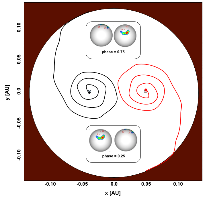
Figure 17: Schematic top-down representation of accretion onto the eclipsing stars in 2M1222$-$57 via streams crossing the inner hole in the circumbinary disk. Small circles representing the two stars are to scale relative to their separation. The size of the cavity relative to the orbital semi-major axis is also to scale, inspired by the simulations of Artymowicz & Lubow (1996). Insets represent the accretion footpoints on the two stars as seen by the observer at the two quadrature phases (taken from the modeling of Espaillat et al., 2021, for the accretion footpoints observed in the young star GM Aur). The observer is in the direction of the bottom of the sketch.

In Figure 17 we offer a schematic depiction that may characterize the situation. The essential features of this conceptual sketch are the following: (1) the eclipsing binary sits in a cleared cavity or hole within a circumbinary disk that is presumably responsible for the infrared excess observed in the SED at 20 $\mu$m (see Figure 9); (2) material from the inner disk falls in toward the central binary, with a cadence equal to the binary orbital period, along streams that are presumably optically thin and thus responsible for the emission in the SED at 10 $\mu$m (see Section 5.3 below); (3) the streams produce hot accretion shocks on the stars’ surfaces, again with a cadence equal to the binary orbit; and (4) these accretion hot spots are produced synchronously on the two stars but, due to the high inclination of the orbital plane to the line of sight and the synchronous rotation of the stars, only one star’s spot is preferentially seen at one orbital quadrature and vice-versa. For an example of realistic accretion spots, we draw on recent work by Espaillat et al. (2021) that mapped the detailed structure of the accretion footpoints on GM Aur, a classical T Tauri star; for conceptual simplicity, in Figure 17 we simply reproduce the GM Aur accretion hot spot mapping for both stars but at opposite rotational phases. To be clear, we do not expect that these accretion footpoint “spots” are the same as the (presumably dark) spots responsible for the rotational modulation discussed in Section 4.3. That variability dominates the overall amplitude of variations in the TESS light curve and is coherent over the multi-year timescale of the TESS observations, whereas the accretion variability is highly stochastic and manifests itself principally in the H$\alpha$ full-width at 10% intensity (see Figure 16).

Finally, in light of the evidence for ongoing accretion in the system, it is reasonable to assume that the system experienced accretion in the past, and we may ask whether the accretion history could have affected the stellar properties (see, e.g., the models of Baraffe et al., 2017; Vorobyov et al., 2017). Stassun et al. (2014) considered whether these models could explain some of the discrepancies between standard model predictions and the observed properties of the available sample of PMS EBs, concluding that in general the predicted effects of accretion (i.e., undersized radii, increased $T_{\rm eff}$, under-luminosity, and enhanced Li depletion) were not consistent with the observed effects confronting many low-mass PMS EBs (i.e., inflated radii, suppressed $T_{\rm eff}$, and decreased Li depletion). In the present case, for example, the models of Baraffe et al. (2017) predict for the 2M1222$-$57 primary a radius of $\approx$0.88 R_⊙ (10% smaller than observed), a $T_{\rm eff}$ of $\approx$4350 K (600 K hotter than observed), and Li depletion $\sim$1.5 dex greater than observed (see Section 5.4).

5.3 Circumbinary disk and accretion streams

The SED of 2M1222$-$57 (Figure 9) shows a $\gtrsim 7\sigma$ excess at 22 $\mu$m, suggesting the presence of warm dust at a blackbody temperature of a few hundred K. For example, the dotted green curve in Figure 9 represents a simple, passive dust disk model from Jensen & Mathieu (1997) with an 0.25 AU inner hole and temperature at the inner edge of $\sim$150 K. Such a model can reproduced the observed 22 $\mu$m excess well, however it does not reproduce the observed $\sim 6\sigma$ excess at 10$\mu$m, and scaling up the same disk model to match the 10$\mu$m excess would produce far too large an excess at 22 $\mu$m.

Therefore, as was the case for the analogous system DQ Tau (see Mathieu et al., 1997), we introduce a small amount of optically thin, hot dust within the hole of the circumbinary disk model. As shown by the solid green curve in Figure 9, even just $8\times 10^{-10}$ M_⊙ (i.e., $3\times 10^{-4}$ M_⊕) of dust at 1500 K (corresponding to the dust sublimation temperature) produces a strong 10 $\mu$m silicate emission feature that matches the observed excess. It also produces a small amount of continuum emission in the near-IR that could explain the $2\sigma$ excess observed at 4.5 $\mu$m, though that excess may not be statistically significant.

The need to include hot dust within the circumbinary disk is consistent with the idea that disk material is reaching the inner stars, which necessitates crossing the disk cavity, but not occupying a large cross-section of the cavity so as to produce emission at 10 $\mu$m but not over-produce emission at other wavelengths (see Section 5.2 and Figure 17).

Next, we investigated whether dust at the inner disk edge could potentially explain the residual dips observed in the TESS light curve after removal of the starspot signals (see Section 5.2 and Figure 15). Based on the system geometry, in particular the inclination angle of the orbital plane (Table 3) and assuming a disk cavity 0.25 AU in diameter (see above), we can calculate that the scale-height of the inner disk edge must be $h/r\approx 0.08$ (which corresponds to 2.4 R_⊙) in order to allow disk material to “transit” one of the central stars as seen by the observer. The dips appear to have a typical duration of $\sim$0.1 orbital phase ($\sim$0.3 d), and the Keplerian period at the inner disk edge is $\sim$26.5 d. As seen from the inner disk edge, the disc of one of the central stars subtends an angle of $\sim$3.6^∘, thus material at the disk edge must travel 0.01 of its Keplerian orbit, or $\sim$0.27 d, to transit one of the stars. Thus, an explanation for the observed dips arising from transits by dust at the inner disk edge is fully consistent with the general picture that emerges for the 2M1222$-$57 system (Figure 17). A similar interpretation has been proffered in other young EBs with circumbinary disks exhibiting similar behavior (see, e.g., Terquem et al., 2015).

Finally, recent simulations of orbitally pulsed accretion suggest that the inner binary must possess one or more asymmetries in its physical characteristics (i.e., mass ratio or eccentricity) for the accretion bursts to occur on the orbital period, whereas for a fully symmetric binary ($e=0$, $q=1$) the accretion bursts recur every $\sim$5 orbital periods (see, e.g., Muñoz & Lai, 2016). In 2M1222$-$57, while $e=0$, the stars are evidently of sufficiently different mass ($q\approx 0.9$) to provide the symmetry breaking needed for orbitally pulsed accretion on the orbital period. The tendency for accretion rate variations in 2M1222$-$57 to be greatest on the lower-mass secondary star (see Section 5.2) is also consistent with the simulations (e.g., Shi et al., 2012; Muñoz & Lai, 2016).

5.4 Effects of magnetic activity on stellar properties

We found in Section 5.1 that the precisely measured radii and temperatures of the eclipsing stars in the 2M1222$-$57 system are very well fit at the age of LCC by PMS evolutionary models that account for the effects on stellar structure by magnetic fields (Figure 14). In contrast, the temperatures and radii cannot both be simultaneously fit by standard PMS evolutionary models (Figure 13) at any age (the models predict temperatures $\approx$200 K hotter than observed), and that the age implied by those standard models for the measured mass-radius relationship ($\approx$12 Myr) is significantly younger than the age of $16.2\pm 2.2$ Myr for the LCC association to which 2M1222$-$57 belongs (Section 2.2). Put another way, at the age of LCC, the standard models imply that the stars in 2M1222$-$57 are significantly cooler and larger than expected for their masses.

Precisely this combination of effects—so-called radius inflation and temperature suppression—has been observed in other young, low-mass stars that are magnetically active. And there is ample evidence to suggest that the stars in 2M1222$-$57 are indeed magnetically active, including their rapid rotation due to synchronization with the 3.1-day orbital period (Section 3.3), the presence of starspot modulations in the light curve (Section 4.3), and the modulation of accretion diagnostics in a manner that suggests the presence of magnetic accretion footpoints on the stars (Section 5.2).

Based on the low-mass EB 2M0535$-$05 (Stassun et al., 2006, 2007) and a set of well characterized active M-dwarfs in the field, Stassun et al. (2012) developed empirical relationships between a star’s chromospheric activity, as measured by the strength of H$\alpha$ emission, and the degree to which the star’s radius is inflated and its temperature suppressed. The physics underlying those empirical relationships has been suggested to be the reduction of surface flux emitted by a star with magnetically inhibited convective efficiency and/or covered by magnetic starspots, leading to a decreased overall effective temperature, in turn causing an enlarged radius so as to still radiate the luminosity produced in the stellar core (see, e.g., Chabrier et al., 2007; Somers & Stassun, 2017).

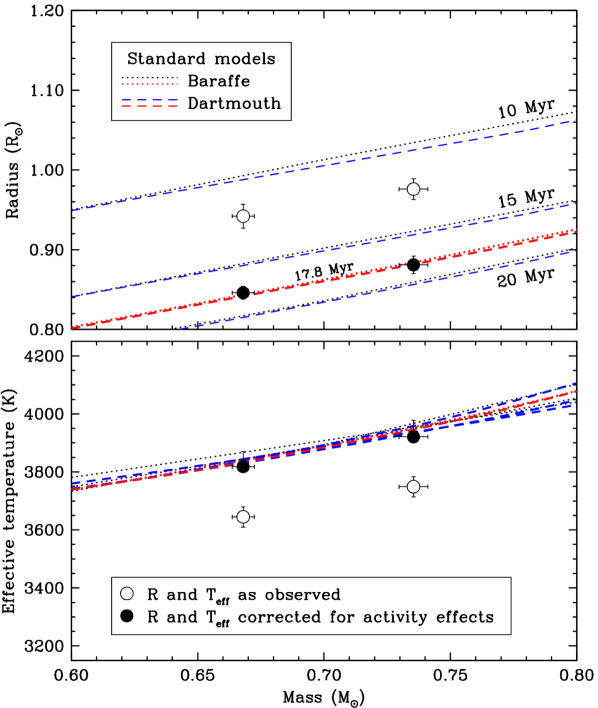
Figure 18: Same as Figure 13 (and on the same scale), now comparing the properties of 2M1222$-$57 before (open symbols) and after (solid symbols) applying the chromospheric activity corrections of Stassun et al. (2012) to the measured temperatures and radii. Now both the radii and temperatures of the two components are well matched by standard theory at an age of $\approx$17 Myr, the same age suggested by the magnetic models (Figure 14). For clarity, the temperatures and radii represented by the solid symbols are not the “true” values; rather, these are what the temperatures and radii would be if the stars were not magnetically active.

Figure 18 shows the result of applying the Stassun et al. (2012) relations to the measured temperatures and radii of the eclipsing stars in 2M1222$-$57. To apply the relations, we used the median H$\alpha$ equivalent widths as an estimate of the basal (presumably chromospheric) emission, to avoid instances of increased H$\alpha$ emission arising from episodic accretion (see Section 5.2 and Figure 16). The agreement of the “activity-corrected” temperatures and radii with the predictions of standard PMS evolutionary models—at an age consistent with the age of LCC—is remarkable, and lends strong support to the idea that strong stellar magnetic fields have significant and measurable effects on the fundamental properties of young stars and on their inferred ages.

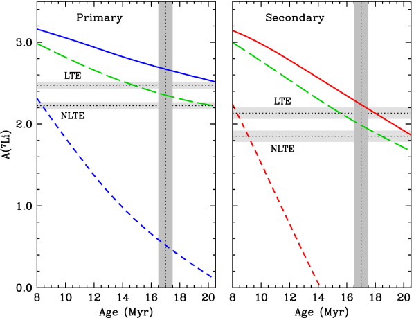
Figure 19: Comparison of Li abundances measured for the primary (left) and secondary (right) eclipsing stars in the 2M1222$-$57 system versus PMS evolutionary model predictions as a function of age; the adopted age of 2M1222$-$57 is represented by the vertical swath. Measured abundances are represented as horizontal swaths for both LTE and NLTE cases (see Section 3.3). Evolutionary tracks for standard PMS models (dashed curves; Baraffe et al., 2015) predict significantly more Li depletion than observed, by $\gtrsim$2 dex, whereas magnetic PMS models (solid curves; Feiden, 2016) are able to much more nearly match the measured values. It is possible to match the Li abundances even better by adjusting the magnetic models with additional parameters, such as with different field strengths for the two stars, represented here by the SPOTS models (Somers et al., 2020) with spot coverage fractions of 24% and 28% for the primary and secondary, respectively (long-dashed green curves).

As a further test of these ideas, we also considered the Li abundances of the eclipsing stars in 2M1222$-$57 in relation to the predictions of magnetic versus standard PMS evolutionary models. First, we converted the measured Li equivalent widths (Section 3.3) into abundances using the curves of growth from Pavlenko & Magazzu (1996), which for the primary give $A({\rm Li})_{1}=2.48\pm 0.04$ dex and $2.23\pm 0.04$ dex for the LTE and NLTE cases, respectively; for the secondary, we obtain $A({\rm Li})_{2}=2.13\pm 0.07$ dex and $1.85\pm 0.07$ dex for the LTE and NLTE cases, respectively. These are represented in Figure 19 in comparison to the same PMS evolutionary models considered above.

It is very clear that the standard models predict significantly more Li depletion at 17 Myr than observed, by $\gtrsim$2 dex. For those models, the observed Li abundances would imply a much younger age of $\sim$8 Myr. It is interesting that this age does not agree with the age of 12 Myr implied by these same models in the mass-radius diagram (see Figure 13). In addition, whereas the standard models are able to reproduce the “activity-corrected” radii and temperatures at an age of 17 Myr (see Figure 18), the same cannot work with the Li abundances; adopting the warmer activity-corrected temperatures would make the observed Li abundances even larger, requiring an even younger inferred age by the standard models.

Thus, while the standard models can predict the global properties (radii and temperatures) of magnetically active stars with suitable adjustments to stellar structure, those models cannot prevent Li from becoming rapidly depleted without an additional change to heat transport in the interior. A similar effect was observed in the PMS EB V1174 Ori (Stassun et al., 2004), which led those authors to conclude that convection in those magnetically active stars was much less efficient than in standard models (see also D’Antona & Montalbán, 2003).

In contrast, the magnetic models are able to reproduce the observed Li abundances reasonably well at an age of 17 Myr. An essential feature of these models is that the same magnetic effects by which the surface temperatures are suppressed and the radii inflated also result in less efficient convective heat transport and a decrease in the temperature at the base of the convection zone, and thus a greatly reduced rate of Li depletion (see, e.g., Somers & Pinsonneault, 2014, 2015a, 2015b; Somers et al., 2020).

The fact that these models perhaps over-predict the Li abundances in 2M1222$-$57 by 0.1–0.2 dex could suggest that a small modification is needed to the interiors physics of the models. For example, a small amount of convective overshoot at the base of the convection zone could in principle produce a small amount of additional Li depletion to match the observed abundances in this case. Alternatively, a slight reduction in the field strength assumed by the models could in principle allow the convective efficiency to be slightly increased and permit a small increase in the Li depletion. For example, the SPOTS magnetic models of Somers et al. (2020) produce too much Li depletion with spot coverage fraction of 17% and too little depletion with spot coverage fraction of 34%, but can be made to match the measured values well with $\sim$25% spot coverage (24% on the primary, 28% on the secondary; see Figure 19).

5.5 The tertiary companion

We conclude with some observations regarding the faint tertiary companion revealed by the speckle observations (Section 3.4). We have very few observational constraints available to characterize the object, other than a brightness contrast relative to the central EB at one wavelength and its contribution to the total light of the system required to be consistent with the third-light determined from the eclipse model (see Section 4.1).

Its angular separation in the speckle imaging places it at a separation of $\sim$100 AU from the central EB, thus presumably it limits the circumbinary disk surrounding the EB to be no larger in extent than $\sim$100 AU. At the nominal 16.2 Myr age of the system, the PMS models of Baraffe et al. (2015) imply a mass of $\sim$0.2 M_⊙, thus placing the object close to but likely above the substellar mass boundary.

More generally, it is interesting that the 2M1222$-$57 system is a hierarchical triple. A large fraction of short-period PMS EBs are now known to be hierarchical triples (see, e.g., Stassun et al., 2014), consistent with the very high prevalence of tertiaries observed among tight spectroscopic binaries in the field (e.g., Tokovinin et al., 2006; Laos et al., 2020).

6 Summary and Conclusions

From TESS light curve observations, we have identified 2M1222$-$57 as a low-mass, pre–main-sequence (PMS) eclipsing binary (EB) with a 3.07-day orbital period. Its membership in the Lower Centaurus Crux (LCC) association provides an opportunity to confront theoretical PMS evolutionary models with the added constraint of an independent age determination. Applying the neural-net age estimator of McBride et al. (2021) to the Gaia astrometry and photometry, we infer an age for LCC and thereby for the 2M1222$-$57 system of 16.2$\pm$2.2 Myr.

There is evidence in the form of excess emission at $\gtrsim$10 $\mu$m for a circumbinary disk around the EB. In addition, speckle-imaging observations reveal a tertiary companion with a photometrically estimated mass of $\sim$0.2 M_⊙ at $\sim$100 AU separation; the tertiary presumably limits the extent of the circumbinary disk to no more than 100 AU. 2M1222$-$57 joins the large fraction of short-period PMS EBs that are hierarchical triples (see, e.g., Stassun et al., 2014).

We observe periodic variations in the H$\alpha$ emission from both stars, in sync with the binary orbital period, which we interpret as accretion streams from the inner edge of the circumbinary disk to the central stars, consistent with theoretical predictions of dynamical interactions between binaries in circumbinary disks (e.g., Artymowicz & Lubow, 1996) and previously reported in observations of some other PMS binaries (e.g., Mathieu et al., 1997; Jensen et al., 2007). Short-duration dips observed in the TESS light curve of 2M1222$-$57 can also be explained by dust at the inner disk edge transiting the central stars, as has been reported for a number of other PMS stars with disks (e.g., Terquem et al., 2015; Rebull et al., 2015; Stauffer et al., 2015).

A joint analysis of the TESS light curve data together with spectroscopically determined radial-velocity measurements and additional tight constraints imposed by the broadband spectral energy distribution (SED) and the Gaia parallax, we determine accurate, empirical masses, radii, and effective temperatures for both eclipsing stars in the system. The $\sim$1% precision achieved on the masses and radii are among the best reported for PMS EBs (see Stassun et al., 2014, for a review). Importantly, thanks to the extremely precise parallax supplied by Gaia, and following the precepts of Miller et al. (2020), we are able to achieve similarly good precision on the effective temperatures. This is important because traditionally it has been the systematic uncertainty on $T_{\rm eff}$ (typically $\sim$100 K; see Torres et al., 2010; Stassun & Torres, 2016) that has been the limiting factor in the ability of EBs to fully stress-test models.

Armed with these extremely precise measurements of both stars’ masses, radii, temperatures, and independently estimated system age, we find that standard PMS stellar evolutionary models (e.g., Baraffe et al., 2015; Feiden, 2016) are unable to simultaneously match the observed radii and temperatures at the age of LCC. Relative to the models, the stars are larger (radius-inflated) and cooler (temperature-suppressed) than predicted for their masses and age. Such effects have been reported among magnetically active low-mass PMS EB stars (e.g., Stassun et al., 2006, 2008), and have been attributed to the reduction of surface flux emitted by a star with magnetically inhibited convective efficiency and/or covered by magnetic starspots, leading to a decreased overall effective temperature, in turn causing an enlarged radius so as to still radiate the luminosity produced in the stellar core (see, e.g., Chabrier et al., 2007; Somers & Stassun, 2017). Indeed, the eclipsing stars in 2M1222$-$57 are clearly magnetically active, as evinced by the presence of rotational starspot modulation signals in the light curve and strong H$\alpha$ emission from both stars in the spectra.

We find that PMS evolutionary models that include the effects of surface magnetic fields (e.g., Feiden, 2016; Somers et al., 2020) are able to reproduce the observed radii and temperatures in 2M1222$-$57 with $\sim$1% precision and at an age that is within 1 Myr of the nominal age of LCC. Moreover, applying the empirical “activity corrections” of Stassun et al. (2012) to the radii and temperatures based on the observed H$\alpha$ strengths—essentially making the stars appear as they would, were they not magnetically active—the standard PMS models are then able to successfully and precisely reproduce the radii and temperatures at the age of LCC. This strongly suggests that the standard models are “correct” insofar as they represent stars without the effects of magnetic activity, and that the magnetic models are “correct” in their implementation of those effects.

These effects are also predicted to alter the interior structure of the stars, with strong implications for the rate at which elements such as Li are depleted. Indeed, we measure the Li abundances of the 2M1222$-$57 stars to be $\sim$2 dex less depleted than predicted by the standard models, whereas the magnetic models are able to much more successfully reproduce the observed abundances. At a more detailed level, we find that the magnetic models of Feiden (2016) slightly over-predict the Li abundances compared to our measurements, possibly suggesting the need for some adjustment to the field strengths assumed in the models (see, e.g., Somers et al., 2020, for an alternative implementation) or in some other aspect of the change in convective efficiency as incorporated in the models.

To a remarkable degree, the 2M1222$-$57 system presents very strong evidence that magnetic activity in young stars alters both their global properties and the physics of their interiors.

References

- Andersen et al. (1980) Andersen, J., Clausen, J. V., & Nordstrom, B. 1980, in Close Binary Stars: Observations and Interpretation, ed. M. J. Plavec, D. M. Popper, & R. K. Ulrich, Vol. 88, 81–86
- Ardila et al. (2015) Ardila, D. R., Jonhs-Krull, C., Herczeg, G. J., Mathieu, R. D., & Quijano-Vodniza, A. 2015, ApJ, 811, 131, doi: 10.1088/0004-637X/811/2/131
- Artymowicz & Lubow (1996) Artymowicz, P., & Lubow, S. H. 1996, ApJ, 467, L77, doi: 10.1086/310200
- Baraffe et al. (2017) Baraffe, I., Elbakyan, V. G., Vorobyov, E. I., & Chabrier, G. 2017, A&A, 597, A19, doi: 10.1051/0004-6361/201629303
- Baraffe et al. (2015) Baraffe, I., Homeier, D., Allard, F., & Chabrier, G. 2015, A&A, 577, A42, doi: 10.1051/0004-6361/201425481
- Basri et al. (1997) Basri, G., Johns-Krull, C. M., & Mathieu, R. D. 1997, AJ, 114, 781, doi: 10.1086/118510
- Binnendijk (1960) Binnendijk, L. 1960, Properties of double stars; a survey of parallaxes and orbits. (University of Pennsylvania Press)
- Bouma et al. (2019) Bouma, L. G., Hartman, J. D., Bhatti, W., Winn, J. N., & Bakos, G. Á. 2019, ApJS, 245, 13, doi: 10.3847/1538-4365/ab4a7e
- Bowler et al. (2019) Bowler, B. P., Hinkley, S., Ziegler, C., et al. 2019, ApJ, 877, 60, doi: 10.3847/1538-4357/ab1018
- Brown (2021) Brown, A. G. A. 2021, ARA&A, 59, 59, doi: 10.1146/annurev-astro-112320-035628
- Chabrier et al. (2007) Chabrier, G., Gallardo, J., & Baraffe, I. 2007, A&A, 472, L17, doi: 10.1051/0004-6361:20077702
- Czekala et al. (2016) Czekala, I., Andrews, S. M., Torres, G., et al. 2016, ApJ, 818, 156, doi: 10.3847/0004-637X/818/2/156
- D’Antona & Montalbán (2003) D’Antona, F., & Montalbán, J. 2003, A&A, 412, 213, doi: 10.1051/0004-6361:20031410
- David et al. (2019) David, T. J., Hillenbrand, L. A., Gillen, E., et al. 2019, ApJ, 872, 161, doi: 10.3847/1538-4357/aafe09
- Dotter et al. (2008) Dotter, A., Chaboyer, B., Jevremović, D., et al. 2008, ApJS, 178, 89, doi: 10.1086/589654
- Eker et al. (2020) Eker, Z., Soydugan, F., Bilir, S., et al. 2020, MNRAS, 496, 3887, doi: 10.1093/mnras/staa1659
- El-Badry et al. (2021) El-Badry, K., Rix, H.-W., & Heintz, T. M. 2021, MNRAS, 506, 2269, doi: 10.1093/mnras/stab323
- Espaillat et al. (2021) Espaillat, C. C., Robinson, C. E., Romanova, M. M., et al. 2021, Nature, 597, 41, doi: 10.1038/s41586-021-03751-5
- Etzel (1981) Etzel, P. B. 1981, in Photometric and Spectroscopic Binary Systems, ed. E. B. Carling & Z. Kopal (Dordrecht: Springer Netherlands), 111–120
- Feiden (2015) Feiden, G. A. 2015, in Astronomical Society of the Pacific Conference Series, Vol. 496, Living Together: Planets, Host Stars and Binaries, ed. S. M. Rucinski, G. Torres, & M. Zejda, 137. https://arxiv.org/abs/1506.02715
- Feiden (2016) Feiden, G. A. 2016, A&A, 593, A99, doi: 10.1051/0004-6361/201527613
- Feiden & Chaboyer (2013) Feiden, G. A., & Chaboyer, B. 2013, ApJ, 779, 183, doi: 10.1088/0004-637X/779/2/183
- Foreman-Mackey et al. (2013) Foreman-Mackey, D., Hogg, D. W., Lang, D., & Goodman, J. 2013, PASP, 125, 306, doi: 10.1086/670067
- Gelman & Rubin (1992) Gelman, A., & Rubin, D. B. 1992, Statistical Science, 7, 457, doi: 10.1214/ss/1177011136
- Gilliland et al. (2010) Gilliland, R. L., Jenkins, J. M., Borucki, W. J., et al. 2010, ApJ, 713, L160, doi: 10.1088/2041-8205/713/2/L160
- Gómez Maqueo Chew et al. (2012) Gómez Maqueo Chew, Y., Stassun, K. G., Prša, A., et al. 2012, ApJ, 745, 58, doi: 10.1088/0004-637X/745/1/58
- Goodman & Weare (2010) Goodman, J., & Weare, J. 2010, Communications in Applied Mathematics and Computational Science, 5, 65, doi: 10.2140/camcos.2010.5.65
- Gregory (2005) Gregory, P. C. 2005, ApJ, 631, 1198, doi: 10.1086/432594
- Howell et al. (2011) Howell, S. B., Everett, M. E., Sherry, W., Horch, E., & Ciardi, D. R. 2011, AJ, 142, 19, doi: 10.1088/0004-6256/142/1/19
- Husser et al. (2013) Husser, T.-O., Wende-von Berg, S., Dreizler, S., et al. 2013, A&A, 553, A6
- Irwin et al. (2011) Irwin, J. M., Quinn, S. N., Berta, Z. K., et al. 2011, ApJ, 742, 123, doi: 10.1088/0004-637X/742/2/123
- Jaehnig et al. (2019) Jaehnig, K., Somers, G., & Stassun, K. G. 2019, ApJ, 879, 39, doi: 10.3847/1538-4357/ab21cf
- Jensen et al. (2007) Jensen, E. L. N., Dhital, S., Stassun, K. G., et al. 2007, AJ, 134, 241, doi: 10.1086/518408
- Jensen & Mathieu (1997) Jensen, E. L. N., & Mathieu, R. D. 1997, AJ, 114, 301, doi: 10.1086/118475
- Kipping (2010) Kipping, D. M. 2010, MNRAS, 408, 1758, doi: 10.1111/j.1365-2966.2010.17242.x
- Kiraga (2012) Kiraga, M. 2012, Acta Astron., 62, 67. https://arxiv.org/abs/1204.3825
- Kounkel (2022) Kounkel, M. 2022, PyXCSAO, 0.2, Zenodo, doi: 10.5281/zenodo.6998993
- Kounkel & Covey (2019) Kounkel, M., & Covey, K. 2019, AJ, 158, 122, doi: 10.3847/1538-3881/ab339a
- Kounkel et al. (2020) Kounkel, M., Covey, K., & Stassun, K. G. 2020, arXiv e-prints, arXiv:2004.07261. https://arxiv.org/abs/2004.07261
- Kurtz & Mink (1998) Kurtz, M. J., & Mink, D. J. 1998, PASP, 110, 934
- Laos et al. (2020) Laos, S., Stassun, K. G., & Mathieu, R. D. 2020, ApJ, 902, 107, doi: 10.3847/1538-4357/abb3fe
- Lindegren et al. (2018) Lindegren, L., Hernández, J., Bombrun, A., et al. 2018, A&A, 616, A2, doi: 10.1051/0004-6361/201832727
- Lindegren et al. (2021) Lindegren, L., Bastian, U., Biermann, M., et al. 2021, A&A, 649, A4, doi: 10.1051/0004-6361/202039653
- Luri et al. (2018) Luri, X., Brown, A. G. A., Sarro, L. M., et al. 2018, A&A, 616, A9, doi: 10.1051/0004-6361/201832964
- MacDonald & Mullan (2014) MacDonald, J., & Mullan, D. J. 2014, ApJ, 787, 70, doi: 10.1088/0004-637X/787/1/70
- Mathieu et al. (1997) Mathieu, R. D., Stassun, K., Basri, G., et al. 1997, AJ, 113, 1841, doi: 10.1086/118395
- McBride et al. (2021) McBride, A., Lingg, R., Kounkel, M., Covey, K., & Hutchinson, B. 2021, The Astronomical Journal, 162, 282, doi: 10.3847/1538-3881/ac2432
- Miller et al. (2020) Miller, N. J., Maxted, P. F. L., & Smalley, B. 2020, MNRAS, 497, 2899, doi: 10.1093/mnras/staa2167
- Muñoz & Lai (2016) Muñoz, D. J., & Lai, D. 2016, ApJ, 827, 43, doi: 10.3847/0004-637X/827/1/43
- Murphy et al. (2020) Murphy, S. J., Lawson, W. A., Onken, C. A., et al. 2020, MNRAS, 491, 4902, doi: 10.1093/mnras/stz3198
- Muzerolle et al. (2019) Muzerolle, J., Flaherty, K., Balog, Z., Beck, T., & Gutermuth, R. 2019, ApJ, 877, 29, doi: 10.3847/1538-4357/ab1756
- Oelkers & Stassun (2018) Oelkers, R. J., & Stassun, K. G. 2018, AJ, 156, 132, doi: 10.3847/1538-3881/aad68e
- Pavlenko & Magazzu (1996) Pavlenko, Y. V., & Magazzu, A. 1996, A&A, 311, 961. https://arxiv.org/abs/astro-ph/9606090
- Popper & Etzel (1981) Popper, D. M., & Etzel, P. B. 1981, AJ, 86, 102, doi: 10.1086/112862
- Preibisch & Mamajek (2008) Preibisch, T., & Mamajek, E. 2008, in Handbook of Star Forming Regions, Volume II, ed. B. Reipurth, Vol. 5 (ASP Monograph Publications), 235
- Prša et al. (2016) Prša, A., Harmanec, P., Torres, G., et al. 2016, AJ, 152, 41, doi: 10.3847/0004-6256/152/2/41
- Rebull et al. (2015) Rebull, L. M., Stauffer, J. R., Cody, A. M., et al. 2015, AJ, 150, 175, doi: 10.1088/0004-6256/150/6/175
- Ricker et al. (2015) Ricker, G. R., Winn, J. N., Vanderspek, R., et al. 2015, Journal of Astronomical Telescopes, Instruments, and Systems, 1, 014003, doi: 10.1117/1.JATIS.1.1.014003
- Scott et al. (2021) Scott, N. J., Howell, S. B., Gnilka, C. L., et al. 2021, Frontiers in Astronomy and Space Sciences, 8, 138, doi: 10.3389/fspas.2021.716560
- Shi et al. (2012) Shi, J.-M., Krolik, J. H., Lubow, S. H., & Hawley, J. F. 2012, ApJ, 749, 118, doi: 10.1088/0004-637X/749/2/118
- Somers et al. (2020) Somers, G., Cao, L., & Pinsonneault, M. H. 2020, ApJ, 891, 29, doi: 10.3847/1538-4357/ab722e
- Somers & Pinsonneault (2014) Somers, G., & Pinsonneault, M. H. 2014, ApJ, 790, 72, doi: 10.1088/0004-637X/790/1/72
- Somers & Pinsonneault (2015a) —. 2015a, ApJ, 807, 174, doi: 10.1088/0004-637X/807/2/174
- Somers & Pinsonneault (2015b) —. 2015b, MNRAS, 449, 4131, doi: 10.1093/mnras/stv630
- Somers & Stassun (2017) Somers, G., & Stassun, K. G. 2017, AJ, 153, 101, doi: 10.3847/1538-3881/153/3/101
- Stassun et al. (2014) Stassun, K. G., Feiden, G. A., & Torres, G. 2014, New A Rev., 60, 1, doi: 10.1016/j.newar.2014.06.001
- Stassun et al. (2012) Stassun, K. G., Kratter, K. M., Scholz, A., & Dupuy, T. J. 2012, ApJ, 756, 47, doi: 10.1088/0004-637X/756/1/47
- Stassun et al. (2008) Stassun, K. G., Mathieu, R. D., Cargile, P. A., et al. 2008, Nature, 453, 1079, doi: 10.1038/nature07069
- Stassun et al. (1999) Stassun, K. G., Mathieu, R. D., Mazeh, T., & Vrba, F. J. 1999, AJ, 117, 2941, doi: 10.1086/300881
- Stassun et al. (2006) Stassun, K. G., Mathieu, R. D., & Valenti, J. A. 2006, Nature, 440, 311, doi: 10.1038/nature04570
- Stassun et al. (2007) —. 2007, ApJ, 664, 1154, doi: 10.1086/519231
- Stassun et al. (2004) Stassun, K. G., Mathieu, R. D., Vaz, L. P. R., Stroud, N., & Vrba, F. J. 2004, ApJS, 151, 357, doi: 10.1086/382353
- Stassun & Torres (2016) Stassun, K. G., & Torres, G. 2016, AJ, 152, 180, doi: 10.3847/0004-6256/152/6/180
- Stassun & Torres (2021) —. 2021, ApJ, 907, L33, doi: 10.3847/2041-8213/abdaad
- Stassun et al. (2019) Stassun, K. G., Oelkers, R. J., Paegert, M., et al. 2019, AJ, 158, 138, doi: 10.3847/1538-3881/ab3467
- Stauffer et al. (2014) Stauffer, J., Cody, A. M., Baglin, A., et al. 2014, AJ, 147, 83, doi: 10.1088/0004-6256/147/4/83
- Stauffer et al. (2015) Stauffer, J., Cody, A. M., McGinnis, P., et al. 2015, AJ, 149, 130, doi: 10.1088/0004-6256/149/4/130
- Stauffer et al. (2017) Stauffer, J., Collier Cameron, A., Jardine, M., et al. 2017, AJ, 153, 152, doi: 10.3847/1538-3881/aa5eb9
- Stauffer et al. (2021) Stauffer, J., Rebull, L. M., Jardine, M., et al. 2021, AJ, 161, 60, doi: 10.3847/1538-3881/abc7c6
- Terquem et al. (2015) Terquem, C., Sørensen-Clark, P. M., & Bouvier, J. 2015, MNRAS, 454, 3472, doi: 10.1093/mnras/stv2258
- Tofflemire et al. (2017a) Tofflemire, B. M., Mathieu, R. D., Ardila, D. R., et al. 2017a, ApJ, 835, 8, doi: 10.3847/1538-4357/835/1/8
- Tofflemire et al. (2017b) Tofflemire, B. M., Mathieu, R. D., Herczeg, G. J., Akeson, R. L., & Ciardi, D. R. 2017b, ApJ, 842, L12, doi: 10.3847/2041-8213/aa75cb
- Tofflemire et al. (2019) Tofflemire, B. M., Mathieu, R. D., & Johns-Krull, C. M. 2019, AJ, 158, 245, doi: 10.3847/1538-3881/ab4f7d
- Tofflemire et al. (2022) Tofflemire, B. M., Kraus, A. L., Mann, A. W., et al. 2022, arXiv e-prints, arXiv:2210.10789. https://arxiv.org/abs/2210.10789
- Tokovinin et al. (2006) Tokovinin, A., Thomas, S., Sterzik, M., & Udry, S. 2006, A&A, 450, 681, doi: 10.1051/0004-6361:20054427
- Torres (2013) Torres, G. 2013, Astronomische Nachrichten, 334, 4, doi: 10.1002/asna.201211743
- Torres et al. (2010) Torres, G., Andersen, J., & Giménez, A. 2010, ARA&A, 18, 67, doi: 10.1007/s00159-009-0025-1
- Vorobyov et al. (2017) Vorobyov, E. I., Elbakyan, V., Hosokawa, T., et al. 2017, A&A, 605, A77, doi: 10.1051/0004-6361/201630356
- White & Basri (2003) White, R. J., & Basri, G. 2003, ApJ, 582, 1109, doi: 10.1086/344673