Machine learning building-block-flow wall model for large-eddy simulation

Abstract

A wall model for large-eddy simulation (LES) is proposed by devising the flow as a combination of building blocks. The core assumption of the model is that a finite set of simple canonical flows contains the essential physics to predict the wall-shear stress in more complex scenarios. The model is constructed to predict zero/favourable/adverse mean pressure gradient wall turbulence, separation, statistically unsteady turbulence with mean flow three-dimensionality, and laminar flow. The approach is implemented using two types of artificial neural networks: a classifier, which identifies the contribution of each building block in the flow, and a predictor, which estimates the wall-shear stress via combination of the building-block flows. The training data are directly obtained from wall-modelled LES (WMLES) optimised to reproduce the correct mean quantities. This approach guarantees the consistency of the training data with the numerical discretisation and the gridding strategy of the flow solver. The output of the model is accompanied by a confidence score in the prediction that aids the detection of regions where the model underperforms. The model is validated in canonical flows (e.g. laminar/turbulent boundary layers, turbulent channels, turbulent Poiseuille–Couette flow, turbulent pipe) and two realistic aircraft configurations: the NASA Common Research Model High-lift and NASA Juncture Flow experiment. It is shown that the building-block-flow wall model outperforms (or matches) the predictions by an equilibrium wall model. It is also concluded that further improvements in WMLES should incorporate advances in subgrid-scale modelling to minimise error propagation to the wall model.

1 Introduction

The use of computational fluid dynamics (CFD) for external aerodynamic applications has been a key tool for aircraft design in the modern aerospace industry (Casey et al., 2000). However, flow predictions from state-of-the-art solvers are still unable to comply with the stringent accuracy requirements and computational efficiency demanded by the industry (Mauery et al., 2021). In recent years, wall-modelled large-eddy simulation (WMLES) has gained momentum as a high-fidelity tool for routine industrial design (Goc et al., 2021). In WMLES, only the large-scale motions in the outer region of the boundary layer are resolved, which enables a competitive computational cost compared with other CFD approaches (Chapman, 1979; Choi & Moin, 2012; Yang & Griffin, 2021). As such, NASA has recognised WMLES as an important pacing item for “developing a visionary CFD capability required by the notional year 2030” (Slotnick et al., 2014). In the present work, we introduce a wall model based on flow-state classification applicable to a wide variety of flow regimes that also provides a confidence score for the prediction.

Several strategies for modelling the near-wall region have been explored in the literature, and comprehensive reviews can be found in Cabot & Moin (2000), Piomelli & Balaras (2002), Spalart (2009), Larsson et al. (2016) and Bose & Park (2018). One of the most widely used approaches for wall modelling is the wall flux approach (or approximate boundary conditions), where the no-slip and thermal wall boundary conditions are replaced with shear stress and heat flux boundary conditions provided by the wall model. This category of wall models utilises the large-eddy simulation (LES) solution at a given location in the domain as input and returns the wall fluxes needed by the solver as boundary conditions. Examples of the most popular approaches are those computing the wall shear stress using the law of the wall (Deardorff, 1970; Schumann, 1975; Piomelli et al., 1989), the full/simplified Reynolds-averaged Navier-Stokes equations (Balaras et al., 1996; Wang & Moin, 2002; Bodart & Larsson, 2011; Kawai & Larsson, 2013; Bermejo-Moreno et al., 2014; Park & Moin, 2014; Yang et al., 2015), structural vortex models (Chung & Pullin, 2009) or dynamic wall models (Bose & Moin, 2014; Bae et al., 2019). Despite the progress, recent results from the American Institute of Aeronautics and Astronautics Workshop on high-lift prediction (Kiris et al., 2022) have evidenced the deficiencies of state-of-the-art WMLES in realistic aircraft. Even simulations with over 350 million degrees of freedom, which are too costly for routine industrial design cycle, are unable to accurately match the experimental results (Rumsey et al., 2019; Lozano-Durán et al., 2022; Goc et al., 2022; GMGW-HLPW, 2022).

The need for improved predictions has incited the adoption of machine learning (ML) tools to complement and enhance existing turbulence models. The reader is referred to the multiple reviews in the literature for a comprehensive overview on ML for fluid mechanics (Duraisamy et al., 2019; Brunton et al., 2020; Brenner et al., 2019; Pandey et al., 2020; Duraisamy, 2021; Beck & Kurz, 2021; Vinuesa & Brunton, 2022; Vinuesa et al., 2022). Most models follow the supervised learning paradigm, i.e., the ML task of learning a function that maps an input to an output based on known input–output pairs. The first ML-based models for LES were introduced in the form of subgrid-scale (SGS) models. Early approaches used artificial neural networks (ANNs) to emulate and speed up a conventional, but computationally expensive, SGS model (Sarghini et al., 2003). More recently, SGS models have been trained to predict the (so-called) perfect SGS terms using data from filtered direct numerical simulation (DNS) (Gamahara & Hattori, 2017; Xie et al., 2019). Other approaches include deriving SGS terms from optimal estimator theory (Vollant et al., 2017), deconvolution operators (e.g. Hickel et al., 2004; Maulik & San, 2017; Fukami et al., 2019) or optimised SGS tensor accounting for numerical errors (Ling et al., 2022).

One of the first attempts at using supervised learning for wall models in LES can be found in Yang et al. (2019). The authors noted that a model trained on turbulent channel flow data at a single Reynolds number could be extrapolated to higher Reynolds numbers in the same configuration. Similar approaches for data-driven wall models using supervised learning were developed for various flow configurations, such as a spanwise rotating channel flow (Huang et al., 2019), flow over periodic hills (Zhou et al., 2021), turbulent flows with separation (Zangeneh, 2021), and boundary layer flow in the presence of shock–boundary layer interaction (Bhaskaran et al., 2021), with mixed results in a posteriori testing. The first attempt at semi-supervised learning for WMLES can be found in Bae & Koumoutsakos (2022), where the authors used reinforcement learning to train on turbulent channel flow data at relatively low Reynolds numbers. The model was able to extrapolate to higher Reynolds numbers for turbulent channel flows and zero pressure gradient turbulent boundary layers. The reinforcement learning wall model has recently been extended to account for pressure gradient effects (Zhou et al., 2022). Nonetheless, most of the models cited above rely on information about the flow that is typically inaccessible in real-world applications, such as the boundary layer thickness, and are limited to simple flow configurations. One exception is the ML wall model introduced by Lozano-Durán & Bae (2020), which is is directly applicable to arbitrary complex geometries and provides the foundations for the present modelling effort.

Currently, one major challenge for WMLES of realistic external aerodynamic applications is achieving robustness and accuracy necessary to model the myriad of different flow regimes that are characteristic of these problems. Examples include turbulence with mean flow three-dimensionality, laminar-to-turbulent transition, flow separation, secondary flow motions at corners, and shock wave formation, to name a few. The wall stress generation mechanisms in these complex scenarios differ from those in flat-plate turbulence. However, the most widespread wall models are built upon the assumption of statistically in equilibrium wall-bounded turbulence without mean flow three-dimensionality, which only applies to a handful number of flows. The latter raises the question of how to devise models capable of seamlessly accounting for such a vast and rich collection of flow physics in a single unified approach. Another important consideration is the data required for training the ML models and consistency with the numerical schemes and grid generation strategy.

In this work, we develop a wall model for LES using building-block flows. The model is formulated to account for various flow configurations, such as wall-attached turbulence, wall turbulence under favourable/adverse pressure gradients, separated turbulence, statistically unsteady turbulence, and laminar flow. The model comprises two components: a classifier and a predictor. The classifier is trained to place the flows into separate categories along with a confidence score, while the predictor outputs the modelled wall stress based on the likelihood of each category. The training data are directly obtained from WMLES with an ‘exact’ model for mean quantities to guarantee consistency with the numerical discretisation and grid structure. The model is validated in canonical flows outside the training set and complex flows. The latter includes two realistic aircraft configurations, namely, the NASA Common Research Model High-lift and NASA Juncture Flow Experiment.

This paper is organised as follows. The formulation of the new model is discussed in §2. The numerical approach and traditional wall models that serves as a comparison point are introduced in §3. The model is validated in §4 and compared with an equilibrium wall model. The model limitations are discussed in §5. Finally, conclusions are offered in §6.

2 Model formulation

The working principle of the proposed model is summarised in figure 1. The model is referred to as the building-block-flow wall model (BFWM) and was first introduced by Lozano-Durán & Bae (2020). The BFWM is comprised of two elements: a classifier and a predictor. First, the classifier is fed data from the LES solver and quantifies the similarities of the input with a collection of known building-block flows. The predictor leverages the information of the classifier together with the input to generate the wall-shear stress prediction via combination of the building-block flows from the database. Each building block is dedicated to modelling different flow physics (e.g. wall-attached turbulence, adverse/favourable pressure-gradient effects, separation, laminar flow), and the model provides a blending between flows using information from the classifier. A confidence score is generated based on the similarity between the input data and the building-block flows. If the input data look extraneous, then the model prompts a low confidence score, which essentially means that the flow is unknown and does not match any knowledge from the database. In the following, we elaborate on the model requirements, assumptions, input/output data, training data, and ANN architecture.

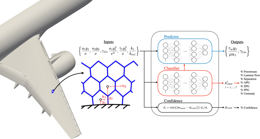
Figure 1: Schematic of the building-block flow wall model (BFWM). Details of the formulation are provided in §2.

2.1 Model requirements

We consider the following model requirements.

1. The wall model should be able to account for different flow physics (e.g. laminar flow, wall-attached turbulence, separated flow) in a unified manner (i.e., the input and output structure of the model must be identical regardless of the case).

2. The model must be scalable to incorporate additional building-block flows if needed in future versions.

3. The model must provide a confidence score in the prediction at each point at the wall.

4. The model formulation must be directly applicable to complex geometries (e.g., realistic aircraft configuration) without any additional modifications. This requirement will constrain the allowable input variables and the parameters used for their non-dimensionalisation (i.e., they will need to be local in space).

5. The model must account for the numerical errors of the schemes employed to integrate the LES equations. This implies that the input data used to train the model must be consistent with the data from the LES solver rather than from filtered DNS.

6. The inputs and outputs of the model must be given in non-dimensional form to comply with dimensional consistency.

7. The model must be invariant under constant space/time translations and rotations of the frame of reference.

8. The model must be Galilean invariant.

2.2 Model assumptions

The main modelling assumptions are as follows.

1. There is a finite set of simple flows (referred to as building-block flows) that contains the essential flow physics to formulate generalisable wall models.

2. The effect of the (missing) near-wall SGS in WMLES of complex flows is representable by a linear combination of the near-wall behaviour of the building-block flows.

3. A set of N non-dimensional model inputs based on local flow quantities is enough to discern among building-block flows, where N is the minimum number of parameters characterising the building-block flow collection.

4. The non-dimensional form of the model inputs/outputs that provides the best predictive capabilities (i.e., interpolation/extrapolation between training cases) is obtained by scaling the variables with the kinematic viscosity and the distance to the wall.

5. The flow information from two contiguous wall-normal locations is enough to predict the wall-shear stress in the vicinity of those locations.

6. History effects for the SGS flow are captured using instantaneous accelerations without the need for additional information from past times.

Assumptions (i) and (ii) imply that the BFWM would provide accurate predictions as long as the (non-universal) large-scale flow motions are resolved by the WMLES grid, and the (smaller-scale) near-wall dynamics resemble the building-block flows or a combination of them. Assumption (iii) stems from the fact that the number of input variables to distinguish among different cases in the building-block flow collection must be, at least, equal to the number of non-dimensional groups required to completely characterise the wall-shear stress across all the building-block flows. For the building-block flows chosen in this work, six parameters are needed to unambiguously identify the wall-shear stress from one particular case (as will be discussed in §2.3). These parameters are global quantities not available to the model. Instead, six non-dimensional inputs using local flow information are fed into the BFWM to predict the wall-shear stress. However, there is no guarantee that these inputs can be used to discern among all possible building-block flows in an univocal manner at all times, and from there comes the need for assumption (iii).

In assumption (iv), it is assumed that the scaling proposed will be the best in all the flow scenarios that the model may encounter, which is not true in general. For example, the current scaling choice will not provide the best performance in the presence of strong compressibility effects, chemically reacting flows or multiphase flows.

Assumptions (v) and (vi) are adopted for the sake of model simplicity. The choice is informed by our previous work in Lozano-Durán & Bae (2020), where a seven-point stencil was used for the input variables compared to the simpler, two-point stencil selected in the present work. It was noted that the seven-point stencil greatly complicated the model implementation without providing important benefits in terms of model performance. There are additional modelling assumptions that are not explicitly stated above. Nonetheless, points (i) to (vi) are the most critical assumptions affecting the model performance.

2.3 Building-block flows

Seven types of building-block flows are considered, and examples are shown in figure 2. All the cases entail an incompressible flow confined between two parallel walls, with the exception of the freestream flow. Cases with additional complexity, such as airfoils, wings, bumps, are intentionally avoided. The rationale behind this choice is that the building blocks should encode the key flow physics to predict more complex scenarios. Hence we intent to avoid case overfitting, i.e. correctly predicting the flow over a wing merely because the model was also trained on similar wings instead of faithfully capturing the flow physics.

For the building blocks, the streamwise, wall-normal and spanwise spatial coordinates are denoted by $x$, $y$ and $z$, respectively. The walls are separated by a distance $2h$. The density is $\rho$, and the dynamic and kinematic viscosities of the fluid are $\mu$ and $\nu$, respectively. In the following, we discuss the configuration and physical motivation behind each building block. We also include in parentheses the label for each building-block flow.

• Freestream (Freestream). A uniform and constant velocity field is used as representative of freestream flows. The main role of this building-block flow is to identify near-wall regions with zero points per boundary layer thickness. In these situations, the BFWM applies a ZPG model (defined below) to estimate the wall stress. The prediction is accompanied by a low confidence score as there is not enough information to provide reliable predictions.

• Wall-bounded laminar flow (Laminar). The near-wall region of a laminar flow is modelled using Poiseuille flow (i.e., parabolic mean velocity profile). The goal of this building block is to allow the prediction of the wall stress in wall-attached laminar scenarios. The case is characterised by the friction Reynolds number $\Rey_{\tau}=u_{\tau}h/\nu$, where $u_{\tau}$ is the friction velocity at the wall, and $h$ is the channel half-height. The range of Reynolds numbers considered is from $\Rey_{\tau}=5$ to $\Rey_{t}au=10^{4}$. A parabolic mean velocity profile is used to analytically predict the stress at the wall.

• Wall-bounded turbulence under zero mean-pressure-gradient (ZPG). Canonical wall turbulence without mean pressure gradient effects is modelled using turbulent channel flows as a building block. The wall stress predictions are provided by an ANN trained for $\Rey_{\tau}=100$ to $\Rey_{\tau}=10,000$ using numerical data (Lozano-Durán & Jiménez, 2014a; Hoyas et al., 2022).

• Wall-bounded turbulence under favourable/adverse mean-pressure-gradient and separation (FPG, APG, and Separation, respectively). We utilise the turbulent Poiseuille–Couette flow as a simplified representation of wall-bounded turbulence subject to favourable and adverse mean pressure gradient effects. The bottom wall is set at rest, and the top wall is set at a constant velocity equal to $U_{t}>0$. A streamwise mean pressure gradient, denoted by $\mathrm{d}P/\mathrm{d}x$, is applied to the flow. Favourable pressure gradient effects are obtained for values of $\mathrm{d}P/\mathrm{d}x$ accelerating the flow in the same direction as the top wall. Adverse pressure gradient conditions are achieved for values of $\mathrm{d}P/\mathrm{d}x$ that accelerate the flow in the opposite direction as the top wall. Flow separation is represented by values of $\mathrm{d}P/\mathrm{d}x$ at which the wall stress at the bottom wall is zero. The different flow regimes are characterised by the two Reynolds numbers $\Rey_{P}=\pm\sqrt{|\mathrm{d}P/\mathrm{d}x|/\rho}h/\nu$ and $\Rey_{U}=U_{t}h/\nu$. The wall stress predictions are provided by an ANN trained for $\Rey_{P}$ from $-1.2\times 10^{3}$ to $1.2\times 10^{3}$, and $\Rey_{U}$ from $5\times 10^{3}$ to $2\times 10^{4}$. New DNS runs were conducted for these cases using the same numerical solver as in previous investigations by our group (Lozano-Durán et al., 2018; Lozano-Durán & Bae, 2019).

• Statistically unsteady wall turbulence with 3-D mean flow (Unsteady). The last building-block flow considered is a turbulent channel flow subject to a sudden spanwise mean pressure gradient $\mathrm{d}P/\mathrm{d}z$. The role of this case is to capture out-of-equilibrium effects due to strong unsteadiness and mean flow three-dimensionality, such as the decrease in the magnitude of the wall stress and the misalignment between the wall stress vector and mean shear vector. Only the initial transient of the flow, where non-equilibrium effects manifest, is considered. The different flow regimes are characterised by the streamwise friction Reynolds number $\Rey_{\tau}=u_{\tau}h/\nu$ before the imposition of $\mathrm{d}P/\mathrm{d}z$ and the ratio of streamwise to spanwise mean pressure gradients $\Pi=(\mathrm{d}P/\mathrm{d}z)/(\mathrm{d}P/\mathrm{d}x)$. The wall stress predictions are provided by an ANN trained for $\Rey_{\tau}=100$ to $1000$ and $\Pi=5$ to $100$ using data from Lozano-Durán et al. (2020b).

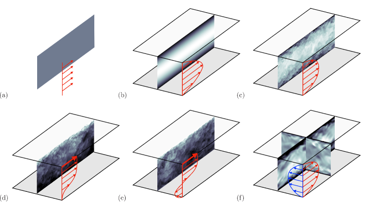
Figure 2: Examples of building-block units taken as representative of different flow regimes: (a) Freestream, (b) laminar channel flow, (c) turbulent channel flow, (d) turbulent Poiseuille–Couette flow for zero wall stress, (e) turbulent Poiseuille–Couette flow with a strong adverse mean pressure gradient, and (f) turbulent channel flow with sudden imposition of spanwise mean pressure gradient.

The wall-shear stress from each case in the building-block flow collection considered is completely determined by the specification of six parameters: Re_τ (or Re_P), $Re_{U}$, $\Pi$, $tu_{\tau}/h$ (non-dimensional time for Unsteady cases), turbulent/non-turbulent flow, and laminar/freestream. Not all parameters are relevant for each case, yet they are required to avoid ambiguities.

The DNS database for ZPG, FPG, APG, Separation, and Unsteady contains roughly 500 simulations. Figure 3 contains examples of the DNS mean velocity profiles for a selection of building-block flows. An advantage of the present building-block set-up is that it allows the generation of contiguous data from one flow regime to another without modifying the geometry but only varying the non-dimensional numbers defining the case (e.g., from FPG to ZPG to APG to Separation by just changing the mean pressure gradient). This facilitates the generation of training data filling the non-dimensional space of inputs, which translates into a more reliable model. The latter is an important requirement, as the role of a model should not be fitting one particular dataset but to learn the scaling of the non-dimensional inputs and outputs controlling the problem at hand.

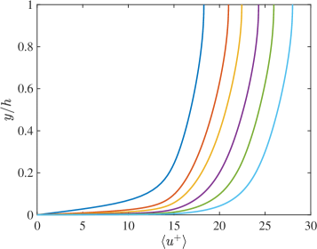
(a)

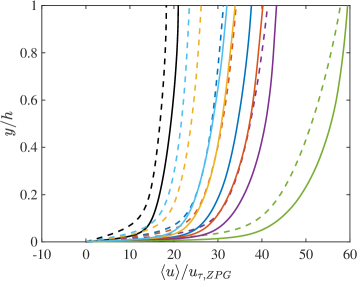
(b)

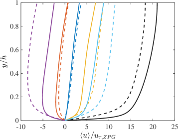
(c)

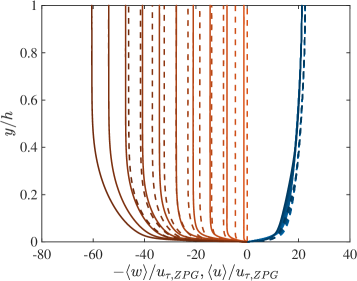
(d)

Figure 3: Mean velocity profiles for a selection of building-block flows. (a) Turbulent channel flows for (from left to right) $\Rey_{\tau}=180,550,950,2000,4200$ and $10,000$ (ZPG). (b) Turbulent Poiseuille–Couette with FPG at $\Rey_{U}=6500$ (dashed) $\Rey_{P}=0,100,150,200,250,300$ (from left to right) and $\Rey_{U}=22,360$ (solid) for $\Rey_{P}=0,380,550,750,800,1000$ (from left to right). (c) Turbulent Poiseuille–Couette with APG and separation at $\Rey_{U}=6500$ (dashed) $\Rey_{P}=0,-100,-150,-200,-250,-300$ (from right to left) and $\Rey_{U}=22,360$ (solid) for $\Rey_{P}=0,-380,-550,-750,-800,-1000$ (from right to left). (d) Turbulent channel flows with the sudden imposition of spanwise mean pressure gradient for increasing time (from light to dark colour) for the streamwise (in blue) and spanwise (in red) mean velocity profiles at $\Rey_{\tau}=550$ (solid) and $\Rey_{\tau}=950$ (dashed) for $\Pi=60$. In all cases, $u_{\tau,ZPG}$ is the friction velocity of the same case without adverse/favourable/spanwise mean pressure gradient.

2.4 Input and output variables

The input variables are acquired using a two-point stencil as shown in figure 1. The stencil contains the centre of the control volume attached to the wall (where the wall-shear stress is to be predicted) and the second control volume off the wall along the wall-normal direction. Given that the model is intended to be used in complex geometries, the centres do not need to align perfectly along the wall-normal direction. This misalignment is considered during the model training. The information collected from the flow is

$$\left\{u_{1},u_{2},\gamma_{12},a_{1},\dot{\gamma}_{1},k_{1},k_{m1}\right\},$$ (1)

where $u_{1}=|\vec{u}_{1}|$ and $u_{2}=|\vec{u}_{2}|$ are the magnitude of the wall-parallel velocities relative to the wall at the first and second control volumes, respectively, $\gamma_{12}$ is the angle between $\vec{u}_{1}$ and $\vec{u}_{2}$, $a_{1}$ is the magnitude of the acceleration at the first control volume, $\dot{\gamma}_{1}$ is the time derivative of the angle of $\vec{u}_{1}$ in the wall-parallel direction, and $k_{1}$ and $k_{m1}$ are the turbulent kinetic energy and mean kinetic energy, respectively, at the first control volume and relative to the wall. The mean velocity to compute $k_{1}$ and $k_{m1}$ is obtained via an exponential average in time (denoted by $(\bar{\cdot})$) with time scale $10\Delta/\sqrt{k_{m1}}$, where $\Delta$ is the characteristic grid size based on the cube root of the control volume. The quantities predicted by the model are

$$\left\{\tau_{w},\gamma_{1w},p_{\mathrm{class}}^{i},p_{\mathrm{conf}}\right\},$$ (2)

where $\tau_{w}=|\vec{\tau}_{w}|$ is the magnitude of the wall stress vector, $\gamma_{1w}$ is the angle between $\vec{u}_{1}$ and $\vec{\tau}_{w}$, $p_{\mathrm{class}}^{i}\in[0,1]$ for $i=1,...,7$ is the probability of the flow corresponding to each building-block category, and $p_{\mathrm{conf}}\in[0,1]$ is the model confidence score.

The input to the wall model comprises the non-dimensional groups formed by the set

$$\left\{\frac{u_{1}y_{1}}{\nu},\frac{u_{2}y_{2}}{\nu},\gamma_{12},\frac{a_{1}y_{1}^{3}}{\nu^{2}},\frac{{\dot{\gamma}}_{1}y_{1}^{2}}{\nu},\frac{k_{1}}{k_{m1}}\right\}.$$ (3)

The model applies the exponential averaged $(\bar{\cdot})$ to the input variables, and this is accounted for in the training. The non-dimensional output of the wall model is

$$\left\{\frac{\tau_{w}y_{1}}{\mu\bar{u}_{1}},\gamma_{1w},p_{\mathrm{class}}^{i},p_{\mathrm{conf}}\right\}.$$ (4)

We have explicitly avoided the use of flow parameters such as freestream velocity, and bulk velocity flow, as they are not unambiguously identifiable for arbitrary geometries.

The non-dimensional groups in (3) are devised to enable the classification and wall stress prediction according to the building-block flows considered. All the inputs contribute to the prediction of the outputs to some degree. However, it is possible to highlight the main role played by each input variable. The first two inputs, $u_{1}y_{1}/\nu$ and $u_{2}y_{2}/\nu$, represent the local Reynolds numbers at the first and second control volumes, respectively. They are key drivers for the prediction of the wall-shear stress in all cases by detecting the shape of the mean velocity profile. They aid the distinction between turbulent channel flow, turbulence with favourable/adverse mean pressure gradient, and separation. The relative angle $\gamma_{12}$ is used to detect three-dimensionality in the mean velocity profile. The non-dimensional acceleration $a_{1}y_{1}^{3}/\nu^{2}$ and the angular rate of change $\dot{\gamma}_{1}y_{1}^{2}/\nu$ facilitate the prediction of the magnitude and direction of statistically unsteady effects in the wall-shear stress. Finally, $k_{1}/k_{m1}$ is leveraged to discern between turbulent flows (ZPG, APG, FPG, etc.) and non-turbulent flows (freestream and laminar). The wall stress at the output is non-dimensionalised using the pseudo-wall-stress $\mu\bar{u}_{1}/y_{1}$, as it was found to minimise the spread of the data between cases. This scaling improved the generalisability of the model and facilitated learning the trends in the data by the ANNs.

2.5 WMLES with optimised SGS/wall model

The training data (discussed in §2.6) are generated using WMLES with SGS/wall models optimised to obtain the exact values for the mean velocity profiles and wall stress distribution in order to attain consistency with the numerical discretisation and gridding strategy of the solver. This approach was preferred over filtered DNS data, as it is known that the SGS tensor in implicitly filtered LES ($\tau^{\mathrm{SGS}}_{ij}$) does not coincide with the Reynolds stress terms resulting from filtering the Navier-Stokes equations. The ambiguity in the filter operator renders DNS data inadequate for the development of SGS models because of inconsistent governing equations (Lund & Kaltenbach, 1995; Lund, 2003; Bae & Lozano-Durán, 2017, 2018, 2022). This limitation is particularly relevant in the present work, as the typical grid sizes utilised in WMLES of external aerodynamics are orders of magnitude larger than the characteristic Kolmogorov length scale of the near-wall turbulence. Consequently, numerical errors are comparable to modelling errors, and the former must be accounted for in order to yield accurate predictions.

We introduce an exact-for-the-mean SGS (ESGS) model given by

$$\tau^{\mathrm{ESGS}}_{ij}=\tau^{\mathrm{base}}_{ij}+\Delta\tau^{\mathrm{SGS}}_{ij},$$ (5)

where $\tau^{\mathrm{base}}_{ij}$ is the SGS stress tensor provided by the baseline (imperfect) SGS model (in this case, the dynamic Smagorinsky model, albeit another model could have been selected), and $\Delta\tau^{\mathrm{SGS}}_{ij}$ is the SGS model correction such that the WMLES mean velocity profiles match the DNS counterparts. In this approach, instantaneous DNS flow fields are not needed, and neither is a specific LES filter shape. The correction $\Delta\tau^{\mathrm{SGS}}_{ij}$ is calculated on the fly as the instantaneous force, $\partial\Delta\tau^{\mathrm{SGS}}_{ij}/\partial x_{j}$, required for $\langle u_{i}\rangle_{xz}=\langle u_{i}^{\mathrm{DNS}}\rangle_{xzt}$, where $\langle\cdot\rangle_{xz}$ denotes average over the homogeneous directions $x$ and $z$, and $\langle u_{i}^{\mathrm{DNS}}\rangle_{xzt}$ is the DNS mean velocity profile for the $i$-th velocity component averaged over $x$, $z$ and $t$. If the DNS flow is not statistically stationary (e.g., the Unsteady building-block flow), then the averaged is taken over $x$, $z$, and statistically equivalent realisations. At each wall-normal location, the force $\partial\Delta\tau^{\mathrm{SGS}}_{ij}/\partial x_{j}$ is numerically calculated as the value required in the right-hand side of the equations to match the DNS mean velocity profile in the next time step.

The boundary condition at the wall is also modified to reproduce the probability density function (p.d.f.) of the wall-shear stress from DNS, and it is referred to as the exact boundary condition (EBC). This was achieved by using an inverse probability integral transform, which generates random numbers from an arbitrary probability distribution given its cumulative distribution function (Devroye, 2006). During runtime of WMLES with EGSG, random numbers are sampled from the uniform distribution and mapped onto the p.d.f. of the wall-shear stress previously obtained from DNS. The process is performed for all wall locations at each time step.

WMLES of all the building-block flows was conducted using ESGS with EBC (hereafter, E-WMLES). The simulations were carried out in the same flow solver later used to implement the BFWM. This guarantees consistency of the training data with the actual numerical errors of the solver and gridding structure under the assumption of an SGS model able to accurately predict the mean velocity profiles.

2.6 E-WMLES training data, ANN architecture, and training method

Figure 4 offers an overview of the training workflow, which is divided into three steps.

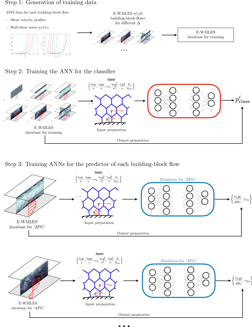
Figure 4: Overview of the training workflow for the BFWM. The details are discussed in §2.6

• Step 1: Generation of E-WMLES training database. The mean velocity profiles and the p.d.f.s of the wall-shear stress from DNS are used to generate the training database using E-WMLES as described in §2.5. The E-WMLES database comprise the building-block flows cases discussed in §2.3 at isotropic grid resolutions $\Delta=h/N$ with $N=5,10,20,40,80,160$ and $380$, which cover (by a wide margin) the grid resolutions encountered in external aerodynamic applications. For grid resolutions finer than $\Delta=h/380$, the BFWM was trained with DNS data to ensure convergence to the no-slip boundary condition. For each grid resolution, the E-WMLES data generated are time-resolved with a varying time step such that the Courant–Friedrichs–Lewy number is equal to 0.5. Time-resolved data were required to compute accelerations and time averages of the input variables that are representative of WMLES. The E-WMLES cases were run for 10 eddy-turnover times (defined by $h/u_{\tau}$). This time was sufficient to capture the statistical trends of the smallest flow scales in the E-WMLES, which have lifetimes of the order of $\Delta/u_{\tau}$ (Lozano-Durán & Jiménez, 2014b). It was found that reducing the time length of the training data below 3 eddy-turnover times significantly reduced the performance of the ANNs. The Unsteady cases were only simulated for the period along which non-equilibrium effects are relevant (i.e., between 0.5 and 2 eddy-turnover times). Each E-WMLES contains of the order of 1,000 to 10,000 snapshots depending on the case. The training set was augmented by performing E-WMLES in which the $x$ direction (i.e., mean flow direction) was rotated parallel to the wall by -45, -40, -35,…, 35, 40 and 45 degrees.

• Step 2: Training the ANN for classifier. The classifier is trained using the full E-WMLES database. classifier The classifier is an ANN with 5 hidden layers and 20 neurons per layer. The layers are connected with rectified linear units (ReLUs) as the activation function. The input to the classifier is the set of non-dimensional groups from Eq. (3). The last layer of the classifier is followed by the softmax activation function, which provides the probabilities of belonging to each building-block flow category ($p_{\mathrm{class}}^{i}$, $i=1,...,7$) such that $\sum p_{\mathrm{class}}^{i}=1$. The network is trained using the Broyden-Fletcher-Goldfarb-Shanno quasi-Newton algorithm (Broyden, 1970; Fletcher, 1970; Goldfarb, 1970; Shanno, 1970; Fletcher, 2013). The performance of the classifier after training is evaluated in figure 5, which shows the normalised confusion matrix. The diagonal of the matrix contains the percentages of inputs that are correctly classified, whereas off-diagonal values show the amount of misclassification among cases. The matrix shows that most samples are correctly classified. There are a few misclassifications (off-diagonal values) which are intentional to ensure a smooth transition between building blocks. This is caused by the overlap between contiguous building blocks, such as Separation and strong APG, mild APG and ZPG, ZPG and mild FPG, and ZPG and Unsteady. The only unintentional misclassification is the larger number of ZPG samples classified as FPG. However, this did not impact the performance of the BFWM, as the wall stress predictions for FPG and ZPG are comparable. Note that there is no ambiguity in the distinction between Freestream/Laminar and turbulent cases, which is important as their predictions vary considerably. A confidence score $p_{\mathrm{conf}}\in[0,1]$ is inferred from the distance of the input to its nearest neighbour in the training set. In particular, the confidence is based on the ratio $d_{s}/d_{i}$ (clipped to be less than 1), where $d_{i}$ is the distance of the input to the closest sample in the training set, and $d_{s}$ is the average distance of the latter to its ten closest samples in the training set.

  

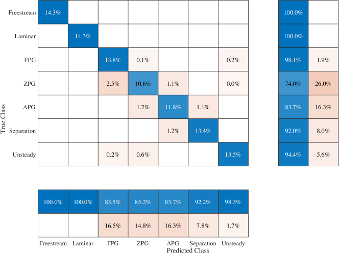
  Figure 5: Confusion matrix of the classifier. The categories are freestream (Freestream), laminar channel flow (Laminar), favourable mean pressure gradient wall turbulence (FPG), zero mean pressure gradient wall turbulence (ZPG), adverse mean pressure gradient wall turbulence (APG), separated turbulence (Separation), and statistically unsteady wall turbulence (Unsteady).

• Step 3: Five ANNs are trained, each dedicated to predict one building-block flow, i.e. ZPG, APG, FPG, Separation, and Unsteady. The ANN predictors are obtained via a deep feed-forward ANN with 5 hidden layers and 30 neurons per layer. The activation functions selected for the hidden layers are hyperbolic tangent sigmoid transfer functions and ReLU activation transfer functions. Predictions of the ANN are calculated for each building-block category and added together, weighted by the probability of belonging to the $i$-th category:

  $$\frac{\tau_{w}y_{1}}{\mu\bar{u}_{1}}=\sum_{i}p_{\mathrm{class}}^{i}\frac{\tau_{w}^{i}y_{1}}{\mu\bar{u}_{1}},\quad\gamma_{1w}=\sum_{i}p_{\mathrm{class}}^{i}\gamma_{1w}^{i},$$ (6)

  where $\tau_{w}^{i}$ and $\gamma_{1w}^{i}$ are the predictions for the $i$-th category. The process is illustrated in figure 6.

  

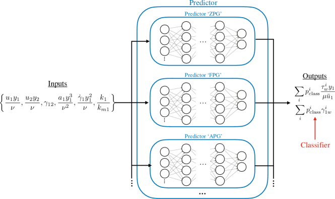
  Figure 6: Schematic of the predictor. The predictor consists of a collection of ANNs/analytical models specialised in predicting the wall-shear stress of each building-block flow. The final output is the sum of the predictions from each building-block flow weighted by the probability of each category.

  The ANNs are trained using Bayesian regularisation back propagation by dividing the training data into two groups: the training set (80% of the data) and the test set (20% of the data). The test set includes full cases for Reynolds numbers (and $\Pi$ values) that are not part of the training set. This was found to improve the predictive capability of the network when interpolating and extrapolating among unseen cases. The errors from each training sample in the lost function were weighted to compensate for the different number of snapshots available for each case. Figure 7 shows the performance plot of the ANN trained for the Unsteady building-block flow.

  

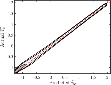
  (a)

  

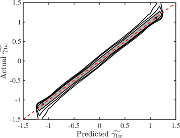
  (b)

  Figure 7: Joint p.d.f. of the predicted output and actual output for (a) themagnitude of the wall stress $\widetilde{\tau_{w}}$, and (b) the relative angle $\widetilde{\gamma_{1w}}$. The tilde denotes values standardised by the mean and standard deviation of the training set. The results are for the statistically unsteady turbulent flow (Unsteady).

For both the classifier and predictor, the inputs and outputs are standardised using the mean and the standard deviation of the training set. These values are stored as part of the model and used to standardise the inputs and outputs when the model is deployed. A parametric study was performed in terms of the number of layers and neurons per layer and the present layouts were found to give a fair compromise between neural network complexity and predictive capabilities. Finally, it took roughly 12 hours to train each ANN using 4 NVIDIA A100 with 40 GB of memory. The computational cost of the WMLES solver using the BFWM is between 1.1 and 1.3 times more expensive than then same WMLES solver using the algebraic equilibrium wall model from §3.2. The particular cost depends on the number of boundary nodes the BFWM is applied to. However, no effort was devoted to optimise the current implementation of the BFWM.

3 Numerical methods

3.1 Flow solver and grid generation

The simulations are conducted with the high-fidelity solver charLES developed by Cascade Technologies, Inc. (Bres et al., 2018; Fu et al., 2021). The code integrates the compressible LES equations using a kinetic-energy-conserving, second-order-accurate, finite-volume method. The numerical discretisation relies on a flux formulation which is approximately entropy-preserving in the inviscid limit, thereby limiting the amount of numerical dissipation added into the calculation. The time integration is performed with a third-order Runge–Kutta explicit method.

The mesh generation follows a Voronoi hexagonal close-packed (HCP) point-seeding method, which automatically builds locally isotropic meshes for arbitrarily complex geometries. First, the watertight surface geometry is provided to describe the computational domain. Second, the coarsest grid resolution in the domain is set to uniformly seeded HCP points. Additional refinement levels are specified in the vicinity of the walls if needed. Ten iterations of Lloyd’s algorithm smooth the transition between layers with different grid resolutions.

3.2 Traditional SGS/wall models

Two SGS models are considered: the dynamic Smagorinsky model (Germano et al., 1991) with the modification by Lilly (1992) (DSM), and the Vreman model (Vreman, 2004) (VRE). For the wall, we use a traditional equilibrium wall model (EQWM). The no-slip boundary condition at the wall is replaced by a wall stress boundary condition. The walls are assumed adiabatic, and the wall stress is obtained by an algebraic equilibrium wall model derived from the integration of the one-dimensional stress model along the wall-normal direction (Deardorff, 1970; Piomelli et al., 1989):

$$u_{2}^{+}(y_{\perp}^{+})=\begin{cases}y_{\perp}^{+}+a_{1}(y_{\perp}^{+})^{2}\text{\, \, \, for $y_{\perp}^{+}<23$},\\ \frac{1}{\kappa}\ln{y_{\perp}^{+}}+B\text{\, \, \, \, otherwise}\end{cases}$$ (7)

where $u_{2}$ is the model wall-parallel velocity at the second grid point off the wall, $y_{\perp}$ is the wall-normal direction to the surface, $\kappa=0.41$ is the Kármán constant, $B=5.2$ is the intercept constant, and $a_{1}$ is computed to ensure $C^{1}$ continuity. The superscript $+$ denotes inner units defined in terms of wall friction velocity and $\nu$.

4 Model validation

The BFWM is first validated in canonical flows: laminar and turbulent boundary layers with zero mean pressure gradient, turbulent pipe flow, turbulent Poiseuille–Couette flows, and statistically unsteady turbulent channel flow. These cases are intended to test the predictive capabilities of the BFWM in flows that are comparable (but not identical) to the training and test sets. The performance of the BFWM to predict the wall-shear stress in complex scenarios is evaluated in two realistic aircraft configurations: the NASA Common Research Model High-lift and the NASA Juncture Flow experiment.

The validation cases are conducted by combining BFWM with two SGS models: DSM and VRE. The simulations performed with DSM and VRE together with BFWM are denoted by DSM-BFWM and VRE-BFWM, respectively. The results are compared with WMLES using DSM and VRE in conjunction with the equilibrium wall model (EQWM). The last two cases are referred to as DSM-EQWM and VRE-EQWM, respectively. When possible, we also include the results for ESGS combined with BFWM (referred to as ESGS-BFWM). The latter aims at assessing the performance of the BFWM in the absence of external SGS modelling errors, as discussed in the following section.

4.1 External versus internal wall-modelling errors

Two sources of errors can be identified in a wall model (Lozano-Durán et al., 2022): errors from the outer LES input data, referred to as external wall-modelling errors, and errors from the wall model physical assumptions, referred to as internal wall-modelling errors. In the former, errors by the SGS model at the matching locations propagate to the value of $\tau_{w}$ predicted by the wall model. These errors can be labelled as external to the wall model inasmuch as they are present even if the wall model provides an exact physical representation of the near-wall region. The second source of errors represents the intrinsic wall model limitations: even in the presence of exact values for the input data, the wall model might incur errors when the physical assumptions of the model do not hold. In the BFWM, internal errors may come from the inadequacy of the building-block flows to represent the physics of the near-wall region (e.g., compressibility effects, heat transfer effects, separation differing from the physics modelled by Poiseuille–Couette flows). A consequence of internal errors is that WMLES might not converge to the DNS solution with grid refinements until the grid is in the DNS-like regime, when the contribution of the wall model is negligible. The combined external plus internal error is referred to as total error. We use ESGS-BFWM to isolate the internal wall-modelling errors when possible.

4.2 Laminar boundary layer

The set-up for the laminar boundary layer is the flow over a flat plate with zero mean pressure gradient and imposed inflow velocity from the Blasius solution. At the top boundary, the freestream velocity is $U_{\infty}$ and the vertical velocity is also calculated from the Blasius solution. A convective boundary condition is used at the outflow. The range of Reynolds numbers is from $\Rey_{x}=U_{\infty}L_{0}/\nu=10^{4}$ to $\Rey_{x}=10^{6}$, where $L_{0}$ is the distance of the inlet to the leading edge of the plate. The streamwise, wall-normal and spanwise sizes of the domain are $150L_{0}\times 2L_{0}\times 1L_{0}$, respectively. The grid resolution is uniform in the three directions, with $\Delta/\delta_{i}\approx 1/2$ at the inlet, which corresponds to $\Delta/\delta_{o}\approx 1/20$ at the outlet, where $\delta_{i}$ and $\delta_{o}$ are the boundary layer thicknesses based on 99% of $U_{\infty}$ at the inlet and outlet, respectively. The reference solution was computed by DNS of the same set-up.

The streamwise mean velocity profiles are captured within 5% error for DSM-EQWM, VRE-EQWM, DSM-BFWM, and VRE-BFWM as shown in figure 8(a). Figure 8(b) reveals that the flow is correctly classified as Laminar with confidence near 100%. The only exception is a small region close to the inlet, where the flow is labelled as Freestream with lower confidence owing to the lack of grid resolution in that region (there are only two points per boundary layer thickness at the inlet). The internal wall model errors are included in figure 8(c), which shows a clear improvement in performance by the BFWM compared to the EQWM. After the initial transient from the inflow, errors for the BFWM are below 1% and decay faster than errors for the EQWM, which are always above 20%. The total wall-stress error is evaluated in figure 8(d). The performance of the BFWM is still superior to that of the EQWM. However, the accuracy of the BFWM is severely diminished due to the external wall-modelling errors from the DSM and VRE. Figure 8(d) also reveals that the DSM-EQWM and VRE-EQWM are subjected to internal/external error cancellation (i.e., predictions may improve despite the fact that input values differ from ESGS). The degraded accuracy of the BFWM due to SGS model errors and the presence of error cancellation using the EQWM are recurrent observations in the following validation cases.

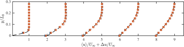
(a)

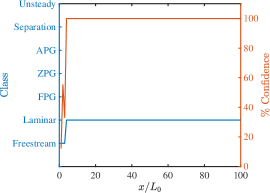
(b)

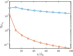
(c)

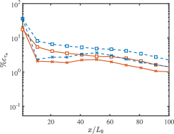
(d)

Figure 8: Validation case: laminar boundary layer. (a) The streamwise mean velocity profiles at $x/L_{0}=1,11,21,31$ and $41$ for the DSM-EQWM (blue squares), VRE-EQWM (blue crosses), DSM-BFWM (red squares), VRE-BFWM (red crosses), and DNS (solid line). The mean velocity profiles are shifted by $\Delta u/U_{\infty}=(x/L_{0}-1)/5$. (b) Dominant flow classification (solid blue) and confidence score (solid red) by the DSM-BFWM as a function of the streamwise distance. (c) Internal wall-modelling error of the wall stress prediction for the ESGS-BFWM (diamonds) and ESGS-EQWM (circles) as a function of the streamwise distance. (d) Total wall-modelling error for the DSM-EQWM (dashed line and squares), DSM-BFWM (solid line and squares), VRE-EQWM (dashed line and crosses), and VRE-BFWM (solid line and crosses) as a function of the streamwise distance.

4.3 Zero mean pressure gradient turbulent boundary layer

For the zero pressure gradient turbulent boundary layer case, the range of $\Rey_{\theta}$ for the turbulent boundary layer is from 800 to 2,000, where $\Rey_{\theta}$ is the Reynolds number based on $U_{\infty}$ and the momentum thickness ($\theta$). The length, height and width of the simulated box are $L_{x}=1060\theta_{\text{avg}}$, $L_{y}=18\theta_{\text{avg}}$, and $L_{z}=35\theta_{\text{avg}}$, where $\theta_{\mathrm{avg}}$ denotes $\theta$ averaged along the streamwise coordinate. The boundary conditions at the top plane are $u=U_{\infty}$, $w=0$, and $v$ is estimated from the known experimental growth of the displacement thickness for the corresponding range of Reynolds numbers as in Jiménez et al. (2010). This controls the average streamwise pressure gradient, whose nominal value is set to zero. The turbulent inflow is generated by the recycling scheme of Lund et al. (1998), in which the velocities from a reference downstream plane, $x_{\text{ref}}$, are used to synthesise the incoming turbulence. The reference plane is located well beyond the end of the inflow region to avoid spurious feedback (Nikitin, 2007; Simens et al., 2009). In our case, $x_{\text{ref}}/\theta_{i}=890$, where $\theta_{i}$ is the momentum thickness at the inlet. A convective boundary condition is applied at the outlet with convective velocity $U_{\infty}$ (Pauley et al., 1990) and small corrections to enforce global mass conservation (Simens et al., 2009). The spanwise direction is periodic. The grid resolution is uniform in the three directions. Compared to the boundary layer thickness, the grid size is $\Delta/\delta_{i}\approx 1/5$ at the inlet and $\Delta/\delta_{o}\approx 1/20$ at the outlet. The reference DNS solution is from Towne et al. (2022), which follows an identical numerical set-up.

To facilitate the comparison between DNS and WMLES, we use as independent variables $\Rey_{x}$ and $x/L_{0}$, as these are free from modelling errors. The streamwise mean velocity profiles (figure 9a) deviate about 10% to 30% from the DNS profile. The flow is correctly classified by the BFWM as ZPG with almost 100% confidence across the vast majority of the domain (figure 9b). Close to the inlet, the flow is labelled as Unsteady and APG, probably because it is still recovering from the artificial inlet boundary condition. From the inlet, the confidence first drops from 40% to 20%, and then recovers up to 100%. In particular, the flow deccelerates close to the inlet under an adverse mean pressure gradient, as seen in the classification of Unsteady and APG. This condition is not explicitly contained in the training set. Therefore, the drop in confidence occurs because the input data to the model move far away from the input data in the training set. After the transient, the flow approaches equilibrium under zero mean pressure gradient, resembling a ZPG turbulent boundary layer. At this point, the flow is identified as ZPG and the confidence increases close to 100%. The internal wall-modelling errors are quantified in figure 9(c), which shows moderate improvements in the performance of the BFWM compared to the EQWM. In particular, the averaged wall stress error is below 0.5% for the BFWM and about 2% for the EQWM once the effect of the inlet condition is forgotten. This case demonstrates that the BFWM is able to successfully interpolate among grid resolutions and Reynolds numbers. In terms of total wall stress error (figure 9d), the BFWM and EQWM exhibit comparable performance, with errors between 5% and 15%. Similar to the previous case, the accuracy of the BFWM worsens due to the external wall-modelling errors when the wall model is coupled with the DSM and VRE.

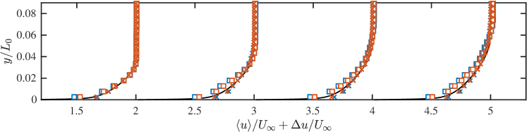
(a)

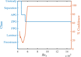
(b)

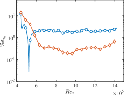
(c)

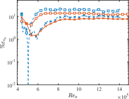
(d)

Figure 9: Validation case: zero mean pressure gradient turbulent boundary layer. (a) The streamwise mean velocity profiles at $\Rey_{x}=6\times 10^{5},8\times 10^{5},10\times 10^{5}$ and $12\times 10^{5}$, for the DSM-EQWM (blue squares), VRE-EQWM (blue crosses), DSM-BFWM (red squares), VRE-BFWM (red crosses) and DNS (solid line). The mean velocity profiles are shifted by $\Delta u/U_{\infty}=(x/L_{0}-1)/5$. (b) Dominant flow classification (solid blue) and confidence score (solid red) by the DSM-BFWM as a function of the streamwise distance. (c) Internal wall-modelling error of the wall stress prediction for the ESGS-BFWM (diamonds) and ESGS-EQWM (circles) as a function of the streamwise distance. (d) Total wall-modelling error for the DSM-EQWM (dashed line and squares), DSM-BFWM (solid line and squares), VRE-EQWM (dashed line and crosses), and VRE-BFWM (solid line and crosses) as a function of the streamwise distance.

4.4 Turbulent pipe flow at $\Rey_{\tau}=40,000$

The next validation case is a turbulent pipe flow at $\Rey_{\tau}\approx 40,000$ with reference data obtained from experiments by Baidya et al. (2019). The flow is driven by a mean streamwise pressure gradient that fixes the Reynolds number based on the centreline velocity to the correct experimental value. The radial coordinate is $r$. The length of the pipe is $100R$, where $R$ is the radius of the pipe, and the streamwise direction is periodic. Four grid resolutions are considered: $\Delta/R\approx 1/5,1/10,1/20,$ and $1/40$.

Figure 10(a) shows that the streamwise mean velocity profiles for the DSM-BFWM and the VRE-BFWM approach the reference data with grid refinement. The flow is accurately classified as ZPG for all the grid resolutions (figure 10b). The BFWM correctly identifies the flow as ZPG with high confidence ($>$95%) for $R/\Delta>5$. For the coarsest grid ($R/\Delta\approx 5$), the flow is also labelled as ZPG but with lower confidence ($<$60%). The latter is the consequence of the poorer performance of the DSM in the coarsest grid resolution, which results in a near-wall mean shear lower than expected from the training set. The internal wall-modelling errors are shown in figure 10(c). Overall, both the BFWM and the EQWM perform satisfactorily, with errors below 5% even at the coarsest grid resolution. This validation case demonstrates that the BFWM successfully extrapolates to high Reynolds numbers for different grid resolutions. The total wall stress error (figure 10d) ranges from 4% to 12% for the BFWM and the EQWM regardless of the SGS model, with a mildly improved accuracy for the BFWM. The results also exhibit the non-monotonic convergence to the true solution typically observed for WMLES in the range of grid resolution considered. This effect, that remains a key issue of WMLES, can be ascribed to the interplay between numerical errors and SGS modelling errors as discussed in Lozano-Durán & Bae (2019) and Lozano-Durán et al. (2022).

(a)

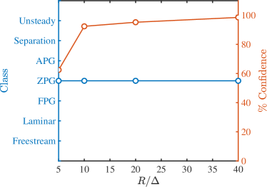
(b)

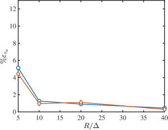
(c)

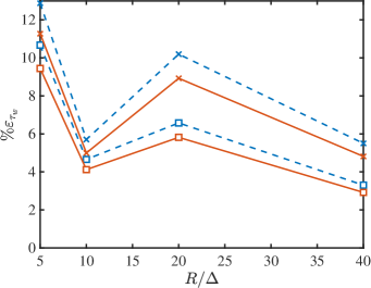
(d)

Figure 10: Validation case: turbulent pipe flow at $\Rey_{\tau}=40,000$. (a) The streamwise mean velocity profiles non-dimensionalised by the mean centreline velocity ($U_{cl}$) for the DSM-BFWM (squares) and VRE-BFWM (crosses) for $R/\Delta\approx$ 5 (blue), 10 (red) and 20 (yellow). The dashed line is the experimental mean velocity profile from Baidya et al. (2019). (b) Dominant flow classification (solid blue) and confidence score (solid red) by the DSM-BFWM as a function of the grid resolution. (c) Internal wall-modelling error of the wall stress prediction for the ESGS-BFWM (diamonds) and ESGS-EQWM (circles) as a function of the grid resolution. (d) Total wall-modelling error for the DSM-EQWM (dashed line and squares), DSM-BFWM (solid line and squares), VRE-EQWM (dashed line and crosses), and VRE-BFWM (solid line and crosses) as a function of the grid resolution.

4.5 Adverse/favourable mean pressure gradient Poiseuille–Couette turbulence

Turbulent Poiseuille–Couette flows at $\Rey_{U}=14,000$ are tested for adverse mean pressure gradients until separation and beyond for $\Rey_{P}\times 10^{-3}=$ -1.40, -1.32, -1.23, -1.13, -1.02, -0.90, -0.76 and $\Rey_{U}=14,000$ and for favourable mean pressure gradients for $\Rey_{P}\times 10^{-3}=1.02,1.13,1.23,1.32,1.41,1.49$. In all cases, the mean streamwise pressure gradient ensures that the Reynolds number based on the centreline velocity matches the correct value. The grid resolution is $h/\Delta=10$. The reference solutions were obtained by DNS. It is worth remarking that these validation cases are not included in the training or testing set discussed in §2.5. Hence the current cases assess the predictive capabilities of the BFWM when both $\Rey_{P}$ and $\Rey_{U}$ are simultaneously varied.

The results for APG/Separation cases and FPG cases are shown in figures 11 and 12, respectively. There are noticeable deviations in the prediction of the mean velocity profiles for both the DSM-EQWM and the VRE-EQWM. Similar results are obtained for their BFWM counterparts. Nonetheless, the flow classification (figures 11b and 12b) is accurate, with a high confidence score ($>90\%$). The internal wall-modelling errors for APG/Separation and FPG cases are shown in figures 11(c) and 12(c), respectively. For the APG/Separation cases, we report the value of the wall-shear stress (rather than the relative error) to avoid dividing by zero close to separation. The BFWM outperforms the EQWM for APG/Separation cases, whereas ZPG cases are all accurately predicted by both wall models, with errors below 3%. The total wall-stress error for APG/separation and FPG cases is shown in figures 11(d) and 12(d), respectively. For APG/Separation, the EQWM provides more accurate predictions than the BFWM, but these are subjected to error cancellation: the EQWM underpredicts the wall-shear stress; however, the mean velocities close to the wall are overpredicted. The combination of both effects results in better predictions for the EQWM, but for the wrong reasons. For FPG, the total error rises from 5% and 20% for increasing favourable pressure gradient. This trend applies to both the BFWM and the EQWM, although the BFWM still outperforms the EQWM.

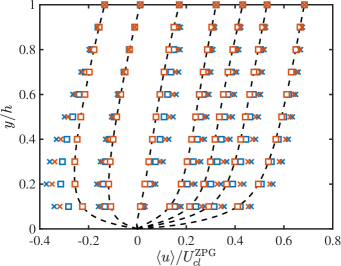
(a)

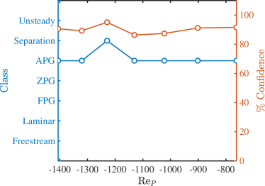
(b)

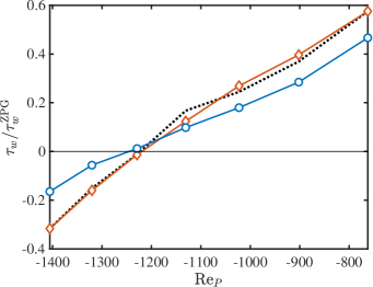
(c)

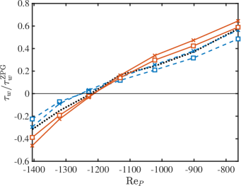
(d)

Figure 11: Validation case: turbulent Poiseuille–Couette flow with adverse mean pressure gradient. (a) The streamwise mean velocity profiles non-dimensionalised by the mean centreline velocity ($U_{cl}^{\mathrm{ZPG}}$) of the case with zero mean pressure gradient for DSM-EQWM (blue squares), VRE-EQWM (blue crosses), DSM-BFWM (red squares) and VRE-BFWM (red crosses) for different $\Rey_{P}$. The dashed lines are mean velocity profiles from DNS. (b) Dominant flow classification (solid blue) and confidence score (solid red) by the DSM-BFWM as a function of the adverse pressure gradient $\Rey_{P}$. (c) Wall stress prediction in the absence of external errors for the ESGS-BFWM (diamonds) and ESGS-EQWM (circles) as a function of $\Rey_{P}$. (d) Total wall stress prediction for the DSM-EQWM (dashed line and squares), DSM-BFWM (solid line and squares), VRE-EQWM (dashed line and crosses), and VRE-BFWM (solid line and crosses) as a function of $\Rey_{P}$. In (c) and (d), the wall stress prediction is non-dimensionalised by the DNS wall stress for the case with zero mean pressure gradient.

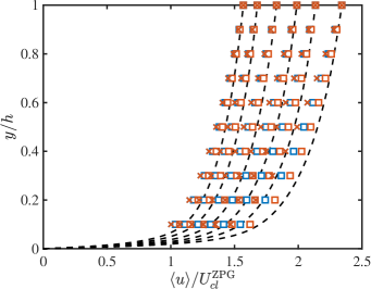
(a)

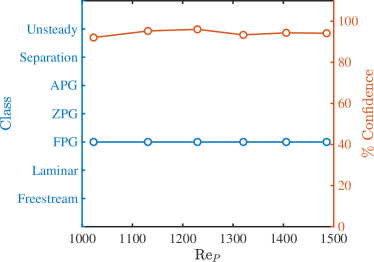
(b)

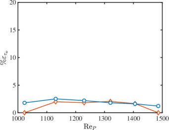
(c)

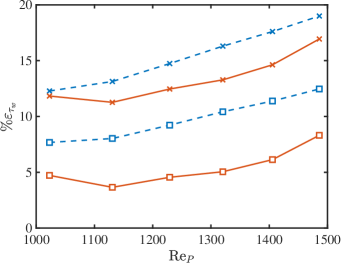
(d)

Figure 12: Validation case: turbulent Poiseuille–Couette flow with favourable mean pressure gradient. (a) The streamwise mean velocity profiles non-dimensionalised by the mean centreline velocity ($U_{cl}^{\mathrm{ZPG}}$) of the case with zero mean pressure gradient for the DSM-EQWM (blue squares), VRE-EQWM (blue crosses), DSM-BFWM (red squares) and VRE-BFWM (red crosses) for different $\Rey_{P}$. The dashed lines are mean velocity profiles from DNS. (b) Dominant flow classification (solid blue) and confidence score (solid red) by the DSM-BFWM as a function of $\Rey_{P}$. (c) Internal wall-modelling error of the wall stress prediction for the ESGS-BFWM (diamonds) and ESGS-EQWM (circles) as a function $\Rey_{P}$. (d) Total wall-modelling error for the DSM-EQWM (dashed line and squares), DSM-BFWM (solid line and squares), VRE-EQWM (dashed line and crosses), and VRE-BFWM (solid line and crosses) as a function of $\Rey_{P}$.

4.6 Turbulent channel flow with the sudden imposition of spanwise pressure gradient

The last canonical validation case is a turbulent channel flow with the sudden imposition of a mean spanwise pressure gradient. The ratio of spanwise to streamwise mean pressure gradient is $\Pi=80$. The grid resolution is $h/\Delta=10$. The simulation is started from a turbulent channel flow at a statistically steady state with $\Rey_{\tau}=700$ for $t<0$ and the lateral pressure gradient is imposed at time $t=0$.

Figures 13(a,b) show the history of the streamwise and spanwise mean velocity profiles for all cases. Predictions of the mean flow remain accurate within 5% error for the second grid point off the wall. More acute errors are observed for the first grid point off the wall. The classifier accurately detects the change of regime from ZPG to Unsteady at $t=0$ with high confidence (figure 13c). The internal wall-modelling errors for the streamwise ($\tau_{w,x}$) and spanwise ($\tau_{w,z}$) wall stresses are shown in figures 13(d,e), respectively. As expected, the BFWM performs better than the EQWM, with errors below 1% for all times. Additionally, the BFWM is able to predict the mild drop in $\tau_{w,x}$ as a function of time, which is completely missed by the EQWM. A similar conclusion applies to the relative angle between $\vec{u}_{1}$ and $\vec{\tau}_{w}$ (namely, $\gamma_{1w}$). The BFWM correctly predicts the increase and decrease of $\gamma_{1w}$, whereas $\gamma_{1w}$ remains zero for the EQWM essentially by construction of the model. Finally, the BFWM still improves the predictions compared to the EQWM in terms of the total wall stress and $\gamma_{1w}$ errors (figures 13g, h, and i), but with lower accuracy than before due to the presence of external wall-modelling errors.

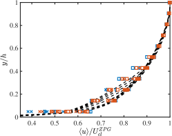
(a)

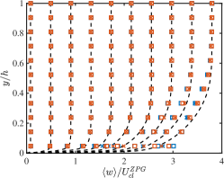
(b)

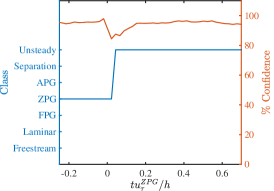
(c)

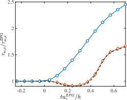
(d)

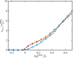
(e)

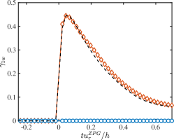
(f)

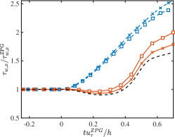
(g)

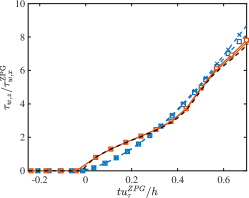
(h)

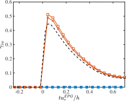
(i)

Figure 13: Validation case: turbulent channel flow sudden imposition of spanwise mean pressure gradient. (a) The streamwise and (b) spanwise mean velocity profiles non-dimensionalised by the centreline mean velocity at $t=0$ ($U_{cl}^{\mathrm{ZPG}}$) for the DSM-EQWM (blue squares), VRE-EQWM (blue crosses), DSM-BFWM (red squares) and VRE-BFWM (red crosses) at $tu_{\tau}^{\mathrm{ZPG}}/h=0.01,0.2,...,0.9$, where $u_{\tau}^{\mathrm{ZPG}}$ is $u_{\tau}$ at $t=0$. The dashed lines are DNS mean velocity profiles (same for all following panels). (c) Dominant flow classification (solid blue) and confidence score (solid red) by the DSM-BFWM as a function of time. Internal wall-modelling error of the (d) streamwise and (e) spanwise wall stress prediction and (f) relative angle between $\vec{u}_{1}$ and $\vec{\tau}_{w}$ for the ESGS-BFWM (diamonds) and ESGS-EQWM (circles) as a function of time. Total wall-modelling error for the streamwise wall stress (g), spanwise wall stress (h), and (i) relative angle between $\vec{u}_{1}$ and $\vec{\tau}_{w}$ for the DSM-EQWM (dashed line and squares), DSM-BFWM (solid line and squares), VRE-EQWM (dashed line and crosses), and VRE-BFWM (solid line and crosses) as a function of time.

4.7 NASA Common Research Model High-lift

The NASA Common Research Model High-lift (CRM-HL) is a geometrically complex aircraft that includes the bracketry associated with deployed flaps and slats as well as a flow-through nacelle mounted on the underside of the wing. The simulations are performed in free air at Reynolds number of 5.49 million based on the mean aerodynamic chord and freestream velocity. The freestream Mach number is 0.20. The results are compared with wind tunnel experimental data from Evans et al. (2020) corrected for free air conditions. Further details of the experimental set-up can be found in Lacy & Sclafani (2016).

We follow the computational set-up from Goc et al. (2021). A semi-span aircraft geometry is simulated, and the symmetry plane is treated with free-slip and no-penetration boundary conditions. Uniform plug flow is used as the inlet. A non-reflecting boundary condition with specified freestream pressure is imposed at the outlet (Poinsot & Lelef, 1992). The total number of grid points is 30 million, and the number of grid points per boundary layer thickness ranges from 0 to 20. The reader is referred to Goc et al. (2021) for more details about the gridding strategy. Figure 14 offers one example of the grid topology. The SGS model is the DSM, and we perform simulations for the DSM-EQWM and the DSM-BFWM. No ESGS model is available for comparison in this case. A summary of previous WMLES of the CRM-HL can be found in Kiris et al. (2022), using traditional SGS and wall models. Here, we re-run the simulations using the DSM-EQWM, and perform new simulations for the DSM-BFWM at angles of attack 7 and 19 degrees.

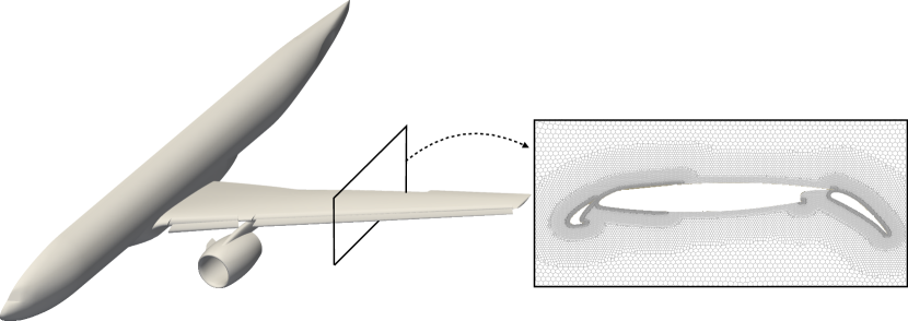
Figure 14: Validation case: NASA Common Research Model High-lift. Geometry of the aircraft (left) and an inset of the grid across the wing section (right).

The lift ($C_{L}$), drag ($C_{D})$ and pitching moment ($C_{M}$) coefficients are shown in figure 15. It is worth remarking that the BFWM has never ‘seen’ an aircraft-like flow or been trained in a case that resembles an aerofoil or a wing. The DSM-BFWM provides moderate improvements with respect to DSM-EQWM, especially close to the stall. The improvements are more clearly manifested in the pitching moment, which is a marker of the accuracy in the force distribution along the wing. The exception is $C_{L}$ at low angles of attack, where the DSM-EQWM outperforms the DSM-BFWM. However, it has been reported that the good predictions by the DSM-EQWM at low angles of attack are coincidental and due to error cancellation, so this should not be taken as a failure of the DSM-BFWM. Despite the improvements by the DSM-BFWM, the results suggest that a superior wall model alone does not suffice to further boost the performance of WMLES unless the SGS model is also improved accordingly.

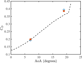
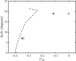
Figure 15: Validation case: NASA Common Research Model High-lift. (a) The lift, (b) drag, and (c) pitching moment coefficients, as a functions of the angle of attack (AoA) for the DSM-BFWM (red circles) and DSM-EQWM (blue circles). The dashed lines are experimental results.

Figure 16 shows the confidence map of BFWM over the surface of the aircraft. Two types of low-confidence ($<$20%) regions are identified. The first region is located at the leading edges of the nacelle, slats and flaps, and is probably related to the lack of grid resolution in those locations (i.e., zero points per boundary layer thickness). The second low-confidence region is related to separation at the wing tip and close to the wing root. This may hint at a lack of grid resolution, the inadequacy of the building-block flows to model separation, or a combination of both. It is worth mentioning that confidence values of 20% still indicate that the flow features detected resemble the building blocks up to some reasonable extent. For example, the presence of completely unknown flow (i.e. random values of the model inputs) will result in confidence scores of 0%. The confidence map is a key feature of the BFWM which enables further evaluation of the model performance. As such, the information from figure 16 might aid grid refinement in poor-confidence regions and/or inform future developments of the model, for example, by suggesting alternative building-block flows or the necessity for new ones.

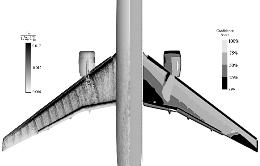
Figure 16: Validation case: NASA Common Research Model High-lift. Visualisation of the instantaneous wall-shear stress (left) and confidence map (right) by the DSM-BFWM.

4.8 NASA Juncture Flow experiment

The NASA Juncture Flow experiment consists of a full-span wing-fuselage body configured with truncated DLR-F6 wings and has been tested in the Langley 14 feet by 22 feet Subsonic Tunnel. The case has been proposed as a validation experiment for generic wing–fuselage junctions at subsonic conditions (Rumsey et al., 2019). The Reynolds number is $\Rey=LU_{\infty}/\nu=2.4$ million, where $L$ is the chord at the Yehudi break. We consider an angle of attack of 5 degrees. The experimental dataset comprises a collection of local-in-space time-averaged measurements (Kegerise et al., 2019), such as velocity profiles and Reynolds stresses, which aid the validation of the BFWM in more detail. The frame of reference is such that the fuselage nose is located at $x=0$, the $x$-axis is aligned with the fuselage centreline, the $y$-axis denotes the spanwise direction, and the $z$-axis is the vertical direction. The associated instantaneous velocities are denoted by $u$, $v$ and $w$.

The SGS model is the DSM, and we perform simulations for the DSM-EQWM and the DSM-BFWM. We use a boundary-layer-conforming grid (Lozano-Durán et al., 2022), such that the control volumes are distributed to achieve five points per boundary layer thickness. Figure 17 contains a visualisation of Voronoi control volumes for the boundary-layer-conforming grid. The reader is referred to Lozano-Durán et al. (2022) for an in-depth description of the computational set-up, numerical methods and grid generation.

Figure 17: Validation case: NASA Juncture flow experiment. Visualisation of Voronoi control volumes for boundary-layer-conforming grid with five points per boundary layer thickness.

The prediction of the mean velocity profiles is shown in figure 18 and compared with experimental measurements. Three locations are considered: the upstream region of the fuselage, the wing–body juncture, and the wing–body juncture close to the trailing edge. Table 1 contains information about the flow classification and confidence in the solution at each location. In the first region, the flow resembles a ZPG turbulent boundary layer. Hence the DSM-EQWM and the DSM-BFWM perform accordingly (i.e., errors below 2%). The flow is identified by the BFWM as 88% ZPG and 12% FPG with $98\%$ confidence. The outcome is expected as the BFWM was trained in turbulent channel flows and the boundary layer at the fuselage resembles a ZPG.

There is a decline in accuracy by the DSM-EQWM in the wing–body juncture and trailing-edge region, which are dominated by adverse pressure gradient effects in the corner and flow separation at the trailing edge. Lozano-Durán et al. (2022) have shown that not only does the DSM-EQWM exhibit larger errors in the wing–body juncture and trailing-edge region, but the rate of convergence of the DSM-EQWM by merely refining the grid is too slow to compensate for the modelling deficiencies at a reasonable computational cost.

The DSM-BFWM provides better predictions in the juncture location compared to the DSM-EQWM. The main reason for the improved results comes from the augmentation of the wall stress compared to the EQWM. This effect accumulates along the streamwise direction, decelerating the flow and alleviating the overprediction of $u$ and $w$ observed with the EQWM. The flow in the juncture is classified as 52% APG and 41% ZPG, which shows that the increase in accuracy is mostly due to the use of the APG building-block flow. The confidence in the prediction is above 80%.

The performance of the DSM-BFWM in the separated region is also improved compared to the DSM-EQWM, but it is still far from satisfactory. The DSM-BFWM classifies the flow as a mix of ZPG, APG and Separation, the latter being the most dominant class (56%). The improvements with respect to the EQWM are caused not only by the use of the APG and Separation building-block flows, but also the improved streamwise history of the flow discussed above. Interestingly, the model prompts a warning about its potential poor performance, which is evidenced by the low confidence ($\sim$20%) in the wall-stress prediction. The deficient performance of the DSM-BFWM and the DSM-EQWM is not surprising if we note that the separation zone has wall-normal thickness 0.3$\delta$ (with $\delta$ the boundary layer thickness), whereas the WMLES grid size is $\Delta\approx 0.2\delta$. Thus there is only one grid point across the separation bubble. Despite the fact that the model was trained in separated flows, the external SGS model errors dominate the LES solution in this case. These errors hinder the capability of the BFWM to correctly classify and predict the flow. Nonetheless, the improvements from BFWM and its ability to assess the confidence in the prediction is a competitive advantage with respect to traditional wall models.

Simulations of the NASA Juncture Flow experiment were also performed by Lozano-Durán & Bae (2020) using a preliminary version of the BFWM trained with filtered DNS data and a smaller collection of building-block flows. The current version of the BFWM provides higher accuracy in the predictions compared to Lozano-Durán & Bae (2020) because of the enhanced collection of building-block flows and the consistency with the numerical scheme of the flow solver.

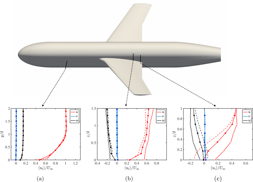
Figure 18: Validation case: NASA Juncture flow experiment. The mean velocity profiles at (a) the upstream region of the fuselage at $x=1168.4$ mm and $z=0$ mm, (b) the wing–body juncture at $x=2747.6$ mm and $y=239.1$ mm, and (c) the wing–body juncture close to the trailing edge at $x=2922.6$ mm and $y=239.1$ mm. Solid lines with open symbols are for the DSM-EQWM, and closed symbols are for the DSM-BFWM. Dashed lines are experiments. Colours denote different velocity components. The distances $y$ and $z$ are normalised by the local boundary layer thickness $\delta$ at each location.

		Location (a)	Location (b)	Location (c)
Classification	Freestream Laminar FPG ZPG APG Separation Unsteady	0% 0% 12% 88% 0% 0% 0%	0% 0% 0% 41% 52% 7% 0%	0% 0% 0% 13% 31% 56% 0%
Confidence		98%	82%	22%

Table 1: Validation case: NASA Juncture flow. The flow classification and confidence in the solution by BFWM. The locations are (a) upstream region of the fuselage, (b) wing-body juncture, and (c) wing-body juncture close to the trailing edge.

5 Model limitations

We close this work by discussing some of the limitations of the BFWM and potential improvements.

• First, the identification of meaningful building-block flows and the minimum number of blocks required to make accurate predictions remains an open question. The present version of the model uses seven building blocks, which is far from being representative of the rich flow physics that might occur in all complex scenarios (e.g. compressibility effects, shock waves, chemical reactions, multiphase flows, different mean flow three-dimensionalities and separation patterns). Additionally, there is no specific mechanism in the BFWM to faithfully capture the laminar-to-turbulent transition, which is of paramount importance in many applications.

• The confidence score offered by the BLWM is based on the similarities between the input flow features and the building-block flows used in the training set. This implies that low confidence scores may still result in accurate wall stress predictions and vice versa. Moreover, the confidence score does not provide an error bound on the value of the prediction, which would be more representative of the model performance. In that vein, future developments of the model could incorporate uncertainty quantification frameworks to estimate error bounds for the quantities of interest (e.g., Sun & Wang, 2020; Maulik et al., 2020; Morimoto et al., 2022; Lozano-Durán & Arranz, 2022; Rezaeiravesh et al., 2022).

• Consistency between the model and the numerical/gridding schemes is solver-dependent. As such, the BFWM must be re-trained to yield accurate predictions in different flow solvers. However, this inconvenience seems inevitable considering the intimate relationship between numerics, gridding and modelling in implicitly filtered LES.

• A key conclusion of this work is that the main limiting factor in the accuracy of the BFWM predictions originates from external modelling errors due to the poor performance of SGS models. This hints at the necessity for a unified SGS/wall model approach where the building-block flow model is also used to devise a numerically consistent SGS model (referred to as a building-block flow model, BFM). Steps in that direction are already been undertaken by our group, and Ling et al. (2022) have shown that the prediction of the lift, drag and pitching moment coefficients for the CRM-HL in §4.7 are greatly improved in the first version of the BFM.

• The prediction and classification tasks in the BFWM rely on ANNs. In this work, it was found that feedforward ANNs with 5 hidden layers and roughly 20–30 neurons per layer enabled accurate results. However, the neural network architectures utilised here may be far from optimal. Moreover, there was no attempt to optimise the computational efficiency of the ANNs, for example via GPU implementation, and further work should be devoted in this direction.

• Variables from past time steps were not included in the model input. Adding such information has the potential of improving the accuracy of the model predictions, as shown in previous studies in the context of turbulence forecasting via ANNs (Lozano-Durán et al., 2020a; Srinivasan et al., 2019; Nakamura et al., 2021).

6 Conclusions

The prediction of aerodynamic quantities of interest remains among the most pressing challenges for computational fluid dynamics, and it has been highlighted as a Critical Flow Phenomena in the NASA CFD Vision 2030 (Slotnick et al., 2014). The aircraft aerodynamics are inherently turbulent with mean flow three-dimensionality, often accompanied by laminar-to-turbulent transition, flow separation, secondary flow motions at corners, and shock wave formation, to name a few. However, the most widespread wall models are built upon the assumption of canonical flat-plate statistically-in-equilibrium wall turbulence, and do not faithfully account for the wide variety of flow conditions described above. This raises the question of how to devise models capable of accounting for such a vast and rich collection of flow physics in a feasible manner.

In this work, we have developed a wall model for large-eddy simulation by devising the flow as a collection of building blocks whose information enables the prediction of the wall stress. The concept was first introduced by Lozano-Durán & Bae (2020), and it is referred to as the building-block-flow wall model (BFWM). The model relies on the assumption that simple flows contain the essential flow physics to formulate generalisable wall models. Seven types of building-block units were used to train the model accounting for zero/favourable/adverse mean pressure gradient wall turbulence, separation, statistically unsteady turbulence with three-dimensional mean flow, and laminar flow. The approach is implemented using two types of artificial neural networks: a classifier, which identifies the contribution of each building block in the flow; and a predictor, which estimates the wall stress via a combinations of building-block units. The output of the model is accompanied by a confidence score. The latter value aids the detection of areas where the model underperforms, such as flow regions that are not representative of the building blocks used to train the model. This a critical component of the BFWM and is considered a key step for developing reliable models. For example, the present model will provide a low confidence score in the presence of a flow that it has never seen before (e.g. a shock wave), or when the wall model input is located in the freestream. Finally, the model is designed to guarantee consistency with the numerical scheme and the gridding strategy. This was attained by training the model using WMLES data obtained with an optimised SGS model that accounts for the numerical errors of the solver.

The BFWM has been validated in laminar and turbulent boundary layers, turbulent pipe flow, turbulent Poiseuille–Couette flows mimicking favourable/adverse mean pressure gradient effects, and statistically unsteady turbulent channel flow with 3-D mean flow. The performance of the BFWM in complex scenarios was evaluated in two realistic aircraft configurations: the NASA Common Research Model High-lift and the NASA Juncture Flow experiment. The validation cases were conducted by combining the BFWM with two SGS models: the dynamic Smagorinsky model and the Vreman model. The BFWM outperforms the traditional equilibrium wall model in canonical cases and the two realistic aircraft scenarios. The only exceptions are the coincidental accurate predictions by the equilibrium wall model due to error cancellation. Despite the improved performance of the BFWM, its accuracy deteriorates considerably owing to external errors from the SGS model. This suggests that additional wall model improvements will not suffice to further boost the performance of WMLES unless the SGS model is also improved.

The modelling capabilities demonstrated by the BFWM, and the ability to extend the model to a richer collection of flow conditions, makes the building-block flow approach a realistic contender to overcome the key deficiencies of current CFD methodologies. We have argued that truly revolutionary improvements in WMLES will encompass advancements in numerics, grid generation and wall/SGS modelling. Here, we have focused on wall modelling and its consistency with the numerics and the grid. However, work remains to be done on the SGS modelling front. In a recent work by our group, Ling et al. (2022) extended the building-block flow methodology to the SGS model and showed that the prediction of the lift, drag and pitching moment coefficients in the CRM-HL are greatly improved compared to the BFWM combined with traditional SGS models. There is also a data science component to the problem, such as the need for efficient and reliable machine learning techniques for data classification and regression. However, in our experience, the model performance is mainly controlled by the physical assumptions rather than by the details of the neural network architecture at hand.

7 Acknowledgements

A.L.-D. acknowledges the support of NASA under grant No. NNX15AU93A from a preliminary version of this work. We thank Konrad Goc for providing the grids for the CRM-HL. The authors acknowledge the MIT SuperCloud and Lincoln Laboratory Supercomputing Center for providing HPC resources that have contributed to the research results reported within this paper.

References

- Bae & Koumoutsakos (2022) Bae, H. J. & Koumoutsakos, P. 2022 Scientific multi-agent reinforcement learning for wall-models of turbulent flows. Nat. Commun. 13 (1), 1443.
- Bae & Lozano-Durán (2017) Bae, H. J. & Lozano-Durán, A. 2017 Towards exact subgrid-scale models for explicitly filtered large-eddy simulation of wall-bounded flows. Center for Turbulence Research - Annual Research Briefs pp. 207–214.
- Bae & Lozano-Durán (2018) Bae, H. J. & Lozano-Durán, A. 2018 DNS-aided explicitly filtered LES of channel flow. Center for Turbulence Research - Annual Research Briefs pp. 197–207.
- Bae & Lozano-Durán (2022) Bae, H. J. & Lozano-Durán, A. 2022 Numerical and modeling error assessment of large-eddy simulation using direct-numerical-simulation-aided large-eddy simulation. arXiv preprint p. arXiv:2208.02354.
- Bae et al. (2019) Bae, H. J., Lozano-Durán, A., Bose, S. T. & Moin, P. 2019 Dynamic slip wall model for large-eddy simulation. J. Fluid Mech. 859, 400–432.
- Baidya et al. (2019) Baidya, R., Baars, W. J., Zimmerman, S., Samie, M., Hearst, R. J., Dogan, E., Mascotelli, L., Zheng, X., Bellani, G., Talamelli, A. & et al. 2019 Simultaneous skin friction and velocity measurements in high Reynolds number pipe and boundary layer flows. J. Fluid Mech. 871, 377–400.
- Balaras et al. (1996) Balaras, E., Benocci, C. & Piomelli, U. 1996 Two-layer approximate boundary conditions for large-eddy simulations. AIAA J. 34 (6), 1111–1119.
- Beck & Kurz (2021) Beck, Andrea & Kurz, Marius 2021 A perspective on machine learning methods in turbulence modeling. GAMM-Mitteilungen 44 (1), e202100002, arXiv: https://onlinelibrary.wiley.com/doi/pdf/10.1002/gamm.202100002.
- Bermejo-Moreno et al. (2014) Bermejo-Moreno, I., Campo, L., Larsson, J., Bodart, J., Helmer, D. & Eaton, J. K. 2014 Confinement effects in shock wave/turbulent boundary layer interactions through wall-modelled large-eddy simulations. J. Fluid Mech. 758, 5–62.
- Bhaskaran et al. (2021) Bhaskaran, R., Kannan, R., Barr, B. & Priebe, S. 2021 Science-guided machine learning for wall-modeled large eddy simulation. In 2021 IEEE International Conference on Big Data, pp. 1809–1816. IEEE.
- Bodart & Larsson (2011) Bodart, J. & Larsson, J. 2011 Wall-modeled large eddy simulation in complex geometries with application to high-lift devices. Center for Turbulence Research - Annual Research Briefs pp. 37–48.
- Bose & Moin (2014) Bose, S. T. & Moin, P. 2014 A dynamic slip boundary condition for wall-modeled large-eddy simulation. Phys. Fluids 26 (1), 015104.
- Bose & Park (2018) Bose, S. T. & Park, G. I. 2018 Wall-modeled large-eddy simulation for complex turbulent flows. Annu. Rev. Fluid Mech. 50, 535–561.
- Brenner et al. (2019) Brenner, M. P., Eldredge, J. D. & Freund, J. B. 2019 Perspective on machine learning for advancing fluid mechanics. Phys. Rev. Fluids 4, 100501.
- Bres et al. (2018) Bres, G. A., Bose, S. T., Emory, M., Ham, F. E., Schmidt, O. T., Rigas, G. & Colonius, T. 2018 Large-eddy simulations of co-annular turbulent jet using a Voronoi-based mesh generation framework. In 2018 AIAA/CEAS Aeroacoustics Conference, p. 3302.
- Broyden (1970) Broyden, C. G. 1970 The convergence of a class of double-rank minimization algorithms: 2. the new algorithm. IMA J. Appl. Math. 6 (3), 222–231.
- Brunton et al. (2020) Brunton, S. L., Noack, B. R. & Koumoutsakos, P. 2020 Machine learning for fluid mechanics. Ann. Rev. Fluid Mech. 52 (1), 477–508.
- Cabot & Moin (2000) Cabot, W. H. & Moin, P. 2000 Approximate wall boundary conditions in the large-eddy simulation of high Reynolds number flow. Flow Turbul. Combust. 63, 269–291.
- Casey et al. (2000) Casey, Michael., Wintergerste, Torsten., European Research Community on Flow, Turbulence & Combustion. 2000 ERCOFTAC best practice guidelines: ERCOFTAC special interest group on “quality and trust in industrial CFD”. ERCOFTAC.
- Chapman (1979) Chapman, D. R. 1979 Computational aerodynamics development and outlook. AIAA J. 17 (12), 1293–1313.
- Choi & Moin (2012) Choi, H. & Moin, P. 2012 Grid-point requirements for large eddy simulation: Chapman’s estimates revisited. Phys. Fluids 24 (1), 011702.
- Chung & Pullin (2009) Chung, D. & Pullin, D. I. 2009 Large-eddy simulation and wall modelling of turbulent channel flow. J. Fluid Mech. 631, 281–309.
- Deardorff (1970) Deardorff, J. 1970 A numerical study of three-dimensional turbulent channel flow at large Reynolds numbers. J. Fluid Mech. 41 (1970), 453–480.
- Devroye (2006) Devroye, Luc 2006 Nonuniform random variate generation. Handbooks in operations research and management science 13, 83–121.
- Duraisamy (2021) Duraisamy, Karthik 2021 Perspectives on machine learning-augmented reynolds-averaged and large eddy simulation models of turbulence. Phys. Rev. Fluids 6, 050504.
- Duraisamy et al. (2019) Duraisamy, K., Iaccarino, G. & Xiao, H. 2019 Turbulence modeling in the age of data. Ann. Rev. Fluid Mech. 51 (1), 357–377.
- Evans et al. (2020) Evans, A. N., Lacy, D. S., Smith, I. & Rivers, M. B. 2020 Test summary of the NASA high-lift common research model half-span at QinetiQ 5-metre pressurized low-speed wind tunnel. In AIAA Aviation 2020 FORUM, p. 2770.
- Fletcher (1970) Fletcher, R. 1970 A new approach to variable metric algorithms. Comput. J. 13 (3), 317–322.
- Fletcher (2013) Fletcher, R. 2013 Practical methods of optimization. John Wiley & Sons.
- Fu et al. (2021) Fu, L., Karp, M., Bose, S. T., Moin, P. & Urzay, J. 2021 Shock-induced heating and transition to turbulence in a hypersonic boundary layer. J. Fluid Mech. 909, A8.
- Fukami et al. (2019) Fukami, K., Fukagata, K. & Taira, K. 2019 Super-resolution reconstruction of turbulent flows with machine learning. J. Fluid Mech. 870, 106–120.
- Gamahara & Hattori (2017) Gamahara, M. & Hattori, Y. 2017 Searching for turbulence models by artificial neural network. Phys. Rev. Fluids 2 (5), 054604.
- Germano et al. (1991) Germano, M., Piomelli, U., Moin, P. & Cabot, W. H. 1991 A dynamic subgrid-scale eddy viscosity model. Phys. Fluids A 3 (7), 1760–1765.
- GMGW-HLPW (2022) GMGW-HLPW 2022 4th CFD High Lift Prediction Workshop.
- Goc et al. (2022) Goc, Konrad, Bose, Sanjeeb T & Moin, Parviz 2022 Large eddy simulation of the nasa high-lift common research model. In AIAA SciTech 2022 Forum, p. 1556.
- Goc et al. (2021) Goc, K. A., Lehmkuhl, O., Park, G. I., Bose, S. T. & Moin, P. 2021 Large eddy simulation of aircraft at affordable cost: a milestone in computational fluid dynamics. Flow 1, E14.
- Goldfarb (1970) Goldfarb, D. 1970 A family of variable-metric methods derived by variational means. Math. Comput. 24 (109), 23–26.
- Hickel et al. (2004) Hickel, S., Franz, S., Adams, N. A. & Koumoutsakos, P. 2004 Optimization of an implicit subgrid-scale model for LES. In Proceedings of the 21st International Congress of Theoretical and Applied Mechanics, Warsaw, Poland.
- Hoyas et al. (2022) Hoyas, S., Oberlack, M., Alcántara-Ávila, F., Kraheberger, S. V. & Laux, J. 2022 Wall turbulence at high friction Reynolds numbers. Phys. Rev. Fluids 7, 014602.
- Huang et al. (2019) Huang, X. L. D., Yang, X. I. A. & Kunz, R. F. 2019 Wall-modeled large-eddy simulations of spanwise rotating turbulent channels—comparing a physics-based approach and a data-based approach. Phys. Fluids 31 (12), 125105.
- Jiménez et al. (2010) Jiménez, J., Hoyas, S., Simens, M. P. & Mizuno, Y. 2010 Turbulent boundary layers and channels at moderate Reynolds numbers. J. Fluid Mech. 657, 335–360.
- Kawai & Larsson (2013) Kawai, S. & Larsson, J. 2013 Dynamic non-equilibrium wall-modeling for large eddy simulation at high Reynolds numbers. Phys. Fluids 25 (1), 015105.
- Kegerise et al. (2019) Kegerise, M. A., Neuhart, D., Hannon, J. & Rumsey, C. L. 2019 An experimental investigation of a wing-fuselage junction model in the NASA Langley 14- by 22-foot subsonic wind tunnel. In AIAA Scitech 2019 Forum, p. 0077.
- Kiris et al. (2022) Kiris, C. C., Ghate, A. S., Duensing, J. C., Browne, O. M., Housman, J. A., Stich, G.-D., Kenway, G., Fernandes, L. S. & Machado, L. M. 2022 High-lift common research model: RANS, HRLES, and WMLES perspectives for CLmax prediction using LAVA. In AIAA Scitech 2022 Forum, p. 1554.
- Lacy & Sclafani (2016) Lacy, D. S. & Sclafani, A. J. 2016 Development of the high lift common research model (HL-CRM): A representative high lift configuration for transonic transports. In 54th AIAA Aerospace Sciences Meeting, p. 0308.
- Larsson et al. (2016) Larsson, J., Kawai, S., Bodart, J. & Bermejo-Moreno, I. 2016 Large eddy simulation with modeled wall-stress: recent progress and future directions. Mech. Eng. Rev. 3 (1), 1–23.
- Lilly (1992) Lilly, D. K. 1992 A proposed modification of the Germano subgrid-scale closure method. Phys. Fluids A 4 (3), 633–635.
- Ling et al. (2022) Ling, Y., Arranz, G., Williams, E., Goc, K. A., Griffin, K. P. & Lozano-Duran, A. 2022 Wall-modeled LES based on building-block flows. Center for Turbulence Research - Proceedings of the Summer Program pp. 5–14.
- Lozano-Durán & Arranz (2022) Lozano-Durán, Adrián & Arranz, Gonzalo 2022 Information-theoretic formulation of dynamical systems: Causality, modeling, and control. Phys. Rev. Research 4, 023195.
- Lozano-Durán & Bae (2019) Lozano-Durán, A. & Bae, H. J. 2019 Characteristic scales of Townsend’s wall-attached eddies. J. Fluid Mech. 868, 698–725.
- Lozano-Durán & Bae (2019) Lozano-Durán, A. & Bae, H. J. 2019 Error scaling of large-eddy simulation in the outer region of wall-bounded turbulence. J. Comput. Phys. 392, 532–555.
- Lozano-Durán & Bae (2020) Lozano-Durán, A. & Bae, H. J. 2020 Self-critical machine-learning wall-modeled LES for external aerodynamics. Center for Turbulence Research - Annual Research Briefs pp. 197–210.
- Lozano-Durán et al. (2020a) Lozano-Durán, Adrián, Bae, H. Jane & Encinar, Miguel P. 2020a Causality of energy-containing eddies in wall turbulence. J. Fluid Mech. 882, A2.
- Lozano-Durán et al. (2022) Lozano-Durán, A., Bose, S. T. & Moin, P. 2022 Performance of wall-modeled LES with boundary-layer-conforming grids for external aerodynamics. AIAA J. 60 (2), 747–766.
- Lozano-Durán et al. (2020b) Lozano-Durán, A., Giometto, M. G., Park, G. I. & Moin, P. 2020b Non-equilibrium three-dimensional boundary layers at moderate Reynolds numbers. J. Fluid Mech. 883, A20.
- Lozano-Durán et al. (2018) Lozano-Durán, A., Hack, M. J. P. & Moin, P. 2018 Modeling boundary-layer transition in direct and large-eddy simulations using parabolized stability equations. Phys. Rev. Fluids 3, 023901.
- Lozano-Durán & Jiménez (2014a) Lozano-Durán, A. & Jiménez, J. 2014a Effect of the computational domain on direct simulations of turbulent channels up to . Phys. Fluids 26 (1), 011702.
- Lozano-Durán & Jiménez (2014b) Lozano-Durán, A. & Jiménez, J. 2014b Time-resolved evolution of coherent structures in turbulent channels: characterization of eddies and cascades. J. Fluid Mech. 759, 432–471.
- Lund (2003) Lund, T. S. 2003 The use of explicit filters in large eddy simulation. Comput. Math. App. 46 (4), 603–616.
- Lund & Kaltenbach (1995) Lund, T. S. & Kaltenbach, H. J. 1995 Experiments with explicit filtering for LES using a finite-difference method. Center for Turbulence Research - Annual Research Briefs pp. 91–105.
- Lund et al. (1998) Lund, T. S., Wu, X. & Squires, K. D. 1998 Generation of turbulent inflow data for spatially-developing boundary layer simulations. J. Comp. Phys. 140 (2), 233–258.
- Mauery et al. (2021) Mauery, T., Alonso, J., Cary, A., Lee, V., Malecki, R., Mavriplis, D. andMedic, G., Schaefer, J. & Slotnick, J. 2021 A guide for aircraft certification by analysis. NASA/CR-20210015404.
- Maulik et al. (2020) Maulik, Romit, Fukami, Kai, Ramachandra, Nesar, Fukagata, Koji & Taira, Kunihiko 2020 Probabilistic neural networks for fluid flow surrogate modeling and data recovery. Phys. Rev. Fluids 5, 104401.
- Maulik & San (2017) Maulik, R. & San, O. 2017 A neural network approach for the blind deconvolution of turbulent flows. J. Fluid Mech. 831, 151–181.
- Morimoto et al. (2022) Morimoto, Masaki, Fukami, Kai, Maulik, Romit, Vinuesa, Ricardo & Fukagata, Koji 2022 Assessments of epistemic uncertainty using gaussian stochastic weight averaging for fluid-flow regression. Physica D: Nonlinear Phenomena 440, 133454.
- Nakamura et al. (2021) Nakamura, Taichi, Fukami, Kai, Hasegawa, Kazuto, Nabae, Yusuke & Fukagata, Koji 2021 Convolutional neural network and long short-term memory based reduced order surrogate for minimal turbulent channel flow. Phys. Fluids 33 (2), 025116.
- Nikitin (2007) Nikitin, N. 2007 Spatial periodicity of spatially evolving turbulent flow caused by inflow boundary condition. Phys. Fluids 19 (9), 091703.
- Pandey et al. (2020) Pandey, Sandeep, Schumacher, Jörg & Sreenivasan, Katepalli R. 2020 A perspective on machine learning in turbulent flows. Journal of Turbulence 21 (9-10), 567–584.
- Park & Moin (2014) Park, G. I. & Moin, P. 2014 An improved dynamic non-equilibrium wall-model for large eddy simulation. Phys. Fluids 26 (1), 015108.
- Pauley et al. (1990) Pauley, L. L., Moin, P. & Reynolds, W. C. 1990 The structure of two-dimensional separation. J. Fluid Mech. 220, 397–411.
- Piomelli & Balaras (2002) Piomelli, U. & Balaras, E. 2002 Wall-layer models for large-eddy simulations. Annu. Rev. Fluid Mech. 34, 349–374.
- Piomelli et al. (1989) Piomelli, U., Ferziger, J., Moin, P. & Kim, J. 1989 New approximate boundary conditions for large eddy simulations of wall-bounded flows. Phys. Fluids A 1 (6), 1061–1068.
- Poinsot & Lelef (1992) Poinsot, T.J & Lelef, S.K 1992 Boundary conditions for direct simulations of compressible viscous flows. J. Comput. Phys. 101 (1), 104 – 129.
- Rezaeiravesh et al. (2022) Rezaeiravesh, S., Vinuesa, R. & Schlatter, P. 2022 An uncertainty-quantification framework for assessing accuracy, sensitivity, and robustness in computational fluid dynamics. Journal of Computational Science 62, 101688.
- Rumsey et al. (2019) Rumsey, C. L., Carlson, J. & Ahmad, N. 2019 FUN3D juncture flow computations compared with experimental data. In AIAA Scitech 2019 Forum, p. 0079.
- Sarghini et al. (2003) Sarghini, F., De Felice, G. & Santini, S. 2003 Neural networks based subgrid scale modeling in large eddy simulations. Comput. Fluids 32 (1), 97–108.
- Schumann (1975) Schumann, U. 1975 Subgrid scale model for finite difference simulations of turbulent flows in plane channels and annuli. J. Comp. Phys. 18, 376–404.
- Shanno (1970) Shanno, D. F. 1970 Conditioning of quasi-Newton methods for function minimization. Math. Comput. 24 (111), 647–656.
- Simens et al. (2009) Simens, M. P., Jiménez, J., Hoyas, S. & Mizuno, Y. 2009 A high-resolution code for turbulent boundary layers. J. Comp. Phys. 228 (11), 4218–4231.
- Slotnick et al. (2014) Slotnick, J., Khodadoust, A., Alonso, J., Darmofal, D., Gropp, W., Lurie, E. & Mavriplis, D 2014 CFD vision 2030 study: A path to revolutionary computational aerosciences. Tech. Rep. NASA/CR–2014-218178. NASA.
- Spalart (2009) Spalart, P. R. 2009 Detached-eddy simulation. Annu. Rev. Fluid Mech. 41, 181–202.
- Srinivasan et al. (2019) Srinivasan, P. A., Guastoni, L., Azizpour, H., Schlatter, P. & Vinuesa, R. 2019 Predictions of turbulent shear flows using deep neural networks. Phys. Rev. Fluids 4, 054603.
- Sun & Wang (2020) Sun, Luning & Wang, Jian-Xun 2020 Physics-constrained bayesian neural network for fluid flow reconstruction with sparse and noisy data. Theoretical and Applied Mechanics Letters 10 (3), 161–169.
- Towne et al. (2022) Towne, A., Dawson, S. T. M., Brés, G. A., Lozano-Durán, A., Saxton-Fox, T., Parthasarathy, A., Jones, A. R., Biler, H., Yeh, C.-A., Patel, H. D. & Taira, K. 2022 A database for reduced-complexity modeling of fluid flows. AIAA J. – (-), –.
- Vinuesa & Brunton (2022) Vinuesa, Ricardo & Brunton, Steven L. 2022 Enhancing computational fluid dynamics with machine learning. Nature Computational Science 2 (6), 358–366.
- Vinuesa et al. (2022) Vinuesa, Ricardo, Lehmkuhl, Oriol, Lozano-Durán, Adrián & Rabault, Jean 2022 Flow control in wings and discovery of novel approaches via deep reinforcement learning. Fluids 7 (2), 62.
- Vollant et al. (2017) Vollant, A., Balarac, G. & Corre, C. 2017 Subgrid-scale scalar flux modelling based on optimal estimation theory and machine-learning procedures. J. Turbul. 18 (9), 854–878.
- Vreman (2004) Vreman, A. W. 2004 An eddy-viscosity subgrid-scale model for turbulent shear flow: Algebraic theory and applications. Phys. Fluids 16 (10), 3670–3681.
- Wang & Moin (2002) Wang, M. & Moin, P. 2002 Dynamic wall modeling for large-eddy simulation of complex turbulent flows. Phys. Fluids 14 (7), 2043–2051.
- Xie et al. (2019) Xie, C., Wang, J., Li, H., Wan, M. & Chen, S. 2019 Artificial neural network mixed model for large eddy simulation of compressible isotropic turbulence. Phys. Fluids 31 (8), 085112.
- Yang & Griffin (2021) Yang, X. I. A. & Griffin, K. P. 2021 Grid-point and time-step requirements for direct numerical simulation and large-eddy simulation. Phys. Fluids 33 (1), 015108.
- Yang et al. (2015) Yang, X. I. A., Sadique, J., Mittal, R. & Meneveau, C. 2015 Integral wall model for large eddy simulations of wall-bounded turbulent flows. Phys. Fluids 27 (2), 025112.
- Yang et al. (2019) Yang, X. I. A., Zafar, S., Wang, J.-X. & Xiao, H. 2019 Predictive large-eddy-simulation wall modeling via physics-informed neural networks. Phys. Rev. Fluids 4 (3), 034602.
- Zangeneh (2021) Zangeneh, R. 2021 Data-driven model for improving wall-modeled large-eddy simulation of supersonic turbulent flows with separation. Phys. Fluids 33 (12), 126103.
- Zhou et al. (2022) Zhou, D., Whitmore, M. P., Griffin, K. P. & Bae, H. J. 2022 Multi-agent reinforcement learning for wall modeling in LES of flow over periodic hills. Center for Turbulence Research - Proceedings of the Summer Program .
- Zhou et al. (2021) Zhou, Z., He, G. & Yang, X. 2021 Wall model based on neural networks for LES of turbulent flows over periodic hills. Phys. Rev. Fluids 6 (5), 054610.